81
-A1 7 7 VL PNENT OF A NICRUBURST TURBULENCE MODE O TE JOINT AIRPORT WEATHER STUDIES MIND SHEAR DATA(U) H CHANG ET AL. AM 67 DOT'FA/PN-87/'±2 IUCLSSFIE D TA10513S1F/ 42 L
-A1 7 7 VL PNENT OF A NICRUBURST TURBULENCE MODE O TEJOINT AIRPORT WEATHER STUDIES MIND SHEAR DATA(U)H CHANG ET AL. AM 67 DOT'FA/PN-87/'±2
IUCLSSFIE D TA10513S1F/ 42 L

9 - II
2.02 or
5. ,128 "-~l -+ l3 ,
I III' iL.. HA 2- I-
N
I LF
I.+
-i
,,,II
" .. a'I'1 ' " " ,P Vi
" ," ,p . '%" . .. " . .. . #-.. . .-.- - . ,-." . ." .- " . --.. . %.-; . .-.- . .- .'." 1. .

UTC FILE Cb Is
DOT/FAA/PM-87/12 Development of a MicroburstProgram Engineering Turbulence Model for theand Maintenance Service Joint Airport Weather StudiesWashington, D.C. 20591 Wind Shear Data
OTIC00 EECTE F
Ho-Pen ChangWalter Frost
FWG Associates, Inc.Rt. 2, Box 271-ATullahoma, TN 37388
for
Research Applications ProgramNational Center for Atmospheric ResearchP.O. Box 3000Boulder, CO 80307
Approved f, .
D, ti-,)- ., . .. March 1987
This document is available to the publicthrough the National Technical InformationService, Springfield, Virginia 22161
U.S. Department of TransportationFederal Aviation Administration
S10 2 091
,-,-. .,-, ", ..- ., -, .,.',.. ,,,,,-.•. -. • .- ,'*,,. * .. , *' a- *'- , .. .. .. .. - ,. ,- , -. .,-.\ . . .. .. ..-*

Technical Report Documentation Page
1. Report No. 2.Go~e-nr 'Acce$ $ o~ No. .Reipent 5 S 00 No.
-DOT/FAA/PM-87/ 12 I 'S74. Ti ti am So, et 5 eoor, Da-e
iDevelopment of a Microburst Turbulence Model for March 1987the Joint Airport Weather Studies (JAWS) Wind Shear 5. folOn Orgao,,zo'on .... ze
Data L _______________
7. Author. s,
Ho-Pen Chanq and Walter Frost_______________9 . Performingq 0,gCMi,:ortoo Name 3na Aaares, 10. work, Unit No. 'TRAIS)
FWG AssociatesRt. 2, Box 271A'DFi2- bO -
Tullahoma, TN 27238 _______ ________.
I 2. Spor,,o,,n AgernCy Namne 3rnd ,jare $s
U.S. epartment of Transpr.t..on TcnclRcrFederal Aviation Ainist-rationProgram Engineering and Maintenance Service 4Sooar,ri~g Agen-, Le
Washington, D.C. 20591 1APr- 3 1015. Supplementary Notes
Research performed under Interagency Agreement No. DTFA01-82-Y-10513 bet.,ieen :-neNational Science Foundation and the Federal Aviation Administration.
16. Abstract J
A turbulence model is developed to supplemnent the microburst quasi-steady wind shear rncceestabl ished earl ier from the JAI.-S Doppler radar data sets. The wind shear model is, in ~ea quasi-steady, spatial ly varying wind field. The spati 'al scale of the wind vari ati 1on is on -eorder of 500-750 ft (150-200 m) . Airborne sensor response (i.e., angle of attack, stall1 wi-i-pitot tubes, etc.), structural dynamics, pilot workload, and otner such factors, however,to much higher frequency wind effects. To account for these effects, a "first-cut" turbu" encemodel based on Doppler radar second moment data is presented. Superimposing the turbulentfluctuation from this turbulence model on the quasi-steady JAWS wind field is believed 'o ;rovide%a more realistic simulation of the microburst flow for aviation application.
The Doppler radar second moments or spectral width data from the June 1, July AardAugust 5, 1982, JAWS microburst measurements are analyzed in cons iderabl edeta il Micrcburstturbulence intensity is calculated by subtracting the spectral width broadeninos due to winoshear, antenna motion, and precipitation fall speeds from the radar spectra width.--r-The turbulenceintensity is compared with the in situ measurement from the NASA B-57B aircraft. !sotropy of amicroburst turbulence is quantitatively investigated by comparing the turbulence informiation fromntwo radar stations which observed the microburst at different directions (approximately 900) . Theturbulence energy contained in a microburst is compared with the theoretical models , both Drydenspectrum and von Karman spectrum. By using a curve-fitting technique, a functional form, of themicroburst turbulence intensity is found in terms of the radial distance from the microburstcenter and the height above the ground. Based on these turbulence parameters relevant to amicroburst, a turbulence model is developed to supplement the existing JAWS quasi-steady meanwind data. Finally, the turbulence model is applied to flight simulations of a B721-t pe aircraftapproaching and/or taking off through a JAWS microburst.
17. Key oods 18. , sbu,'o Slate ,r~~
Turbulence, Doppler radar, spectrumn This document is availabie 11o tre publi'c,width, wind shear, Microburst, second through the National Technical Infor:i'ationmoment, curve fitting, radial distance, Service, Springfield, Virginia 22161.flight simulation, approach, departure
Form DOT F 1700.1 '8-72) Reproduction of completed Poqc" authori zed

ACKNOWLEDGMENT
This work is funded by NCAR Subcontract S3011. The authors expresstheir appreciation of this support. Special thanks go to Dr. John McCarthy ofNCAR who monitored the research program.
JAWS is funded partially by NCAR, the National Science Foundation, theFAA through Interagency Agreement DTFAO1-82-Y-10513, NASA through InteragencyAgreement H-59314B, and NOAA through a cooperative agreement with the Programfor Regional Observing and Forecasting Services of NOAA's EnvironmentalResearch Laboratories.
ii

.-.-
TABLE OF CONTENTS
SECTION PAGE
1.0 INTRODUCTION ... .............. ........... . 1
2.0 ANALYSES OF JAWS TURBULENCE DATA . .................. 3
2.1 Definition of Measurements ...... ................ 3
2.2 Analysis of Pulse SD and Wind SD ...... ............ 9
2.3 Comparison of Radar Data and Aircraft Data ... ....... 25
2.4 Microburst Turbulence Parameters ...... ............ 42
2.4.1 Turbulence Intensity ...... .... ..... 42
2.4.2 Turbulence Length Scales .... ............. ... 47
2.4.3 Turbulence Spectrum . .............. 52
3.0 MICROBURST TURBULENCE MODEL AND ITS APPLICATION IN FLIGHTSIMULATION ...... .... ..... .... ..... .. 55 -v
4.0 CONCLUSIONS ..... .... ......................... ... 63
REFERENCES ...... .... ............................ . 64
APPENDIX: NOMENCLATURE USED IN APPROACH/TAKEOFF SIMULATIONS . . . 66
" ..... .. .......
D,x W W P jBy .. . ........ . ..
' t

LIST OF TABLES
TABLE PAGE
1. Three JAWS Microburst Data Sets ....... ................... 5
2. Characteristics of JAWS Doppler Radar ...... ................ 6
3. Gust Gradient Flights of the'NASA B-57B Aircraft During JAWS 1982 . 33
4. FAA Turbulence Model in AC-120-41 ..... .................. .. 43
5. Center of JAWS Microbursts ........ ..................... 43
6. A Functional Form of Turbulence Intensity for 14JL1452 Microburst . . 48
7. Integral Scales ........... .......................... 52
iv

LIST OF FIGURES
FIGURE PAGE v
1. Locations of Three JAWS Microbursts. . ............... 4
2. Definition of Radial Shear Terms, Kr, Ke, and K4 . . . . . . . . ... . . . . 8
3. Contour of Radial Velocity and Pulse SD at Ground Level for 14JL1452Micrnburst from CP-2 ........ ........................ . 10
4. Contour of Radial Velocity and Pulse SD at Level 8 (about 1 km aboveground) for 14JL1452 Microburst from CP-4 ... ............. .... 12
5. Contour of Radial Velocity and Pulse SD at Level 5 (1 km above ground)for 5AU1847 Microburst from CP-4 ..... .................. ... 15
6. Contour of Wind SD at Level 7 (0.9 km above ground) for 14JL1452Microburst from CP-4 and CP-22 ........ ................... 17
7. Contour of Wind SD Difference Between the Measurements from CP-4 andCP-2 Radars at Level 7 (0.9 km above ground) for 14JL1452Microburst ........ .... .... ..... .... .... 19
8. Contour of Pulse SD at Level 7 (0.9 km above ground) for 14JL1452Microburst from CP-4 and CP-2 ................... 20
9. Contour of Pulse SD Difference Between the Measurements from CP-4and CP-2 Radars at Level 7 (0.9 km above ground) for 14JL1452
.
Microburst ......... ............................ ... 22
10. Cumulative Probabilities of ap, w, Aop, and Aaw for 14JL1452Microburst from Both CP-4 and CP-2 ........ ..... .... 23
11. Cumulative Probabilities of at and aw for 14JL1452 Microburst fromBoth CP-4 and CP-2 ......... ........................ . 25
12. Cumulative Probabilities of u a as and aw for 5AU1847Microburst from CP-4 ....... ........... ...... ... 26
13. Cumulative Probabilities of op, at, as, and aw for 30JN1823Microburst from CP-4 ........ ........................ . 27
14. Cumulative Probabilities of Radial Wind Shear Terms, Kr, K , and Ke,for 14JL1452 Microburst for CP-4 ........ ..... ..... 28
15. Cumulative Probabilities of Radial Wind Shear Terms, Kr, K , and Ke, V.
for 14JL1452 Microburst for CP-2 ...... ................. ... 29
16. Cumulative Probabilities of Radial Wind Shear Terms, Kr, K4 , and Ke,for 5AU1847 Microburst for CP-4 .... .... .................. 30
V

FIGURE PAGE
17. Cumulative Probabilities of Radial Wind Shear Terms, Kr, K, and Ke,for 30JN1823 Microburst for CP-4 ............... ... 31
18. Relative Positions of 14JL1452 Microburst and Flight Paths of Runs23, 24, and 25 in Flight 6 of NASA B-57B Aircraft .. ......... .. 34
19. Flight Path Information, Run 24, Flight 6 ... ............. ... 35
20. Flight Path Information, Run 23, Flight 6 .... ............ ... 36
21. Comparison of a with Calculated Turbulence Intensities from NASAB-57B Aircraft Measurement in Run 24 ..... ............. ... 37
22. Comparison of at and aw with Calculated Turbulence Intensities fromNASA B-57B Aircraft Measurement in Run 24 ... ............. ... 38
23. Comparison of at and ow with Calculated Turbulence Intensities fromNASA B-57B Aircraft Measurement in Run 23 ...... ............ 39
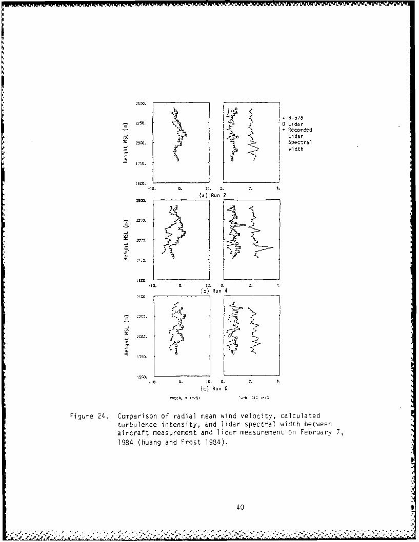
24. Comparison of Radial Mean Wind Velocity, Calculated TurbulenceIntensity, and Lidar Spectral Width Between Aircraft Measurement andLidar Measurement on February 7, 1984 (Huang and Frost 1984) . . . . 40
25. Plots of Radar (solid line) and Aircraft (dotted line) Estimates ofof Spectrum Variance at Grid Points Along Aircraft Track(Bohne 1981) ........ ........................... ... 41
26. Schematic of Sectors and Radial Lines Relative to the MicroburstCenter Along Which Turbulence Intensity was Evaluated . . . . . .. 44
27. Turbulence Intensity at/V Profiles at Different Radial Distancesfrom the Microburst Center for the 14JL1452 Microburst ... ....... 45
28. Curve Fit of the Turbulence Intensity Profiles at/V at DifferentRadial Distances from the Microburst Center for the 14JL1452Microburst ...... ....................................... 46
29. Auto-Correlation Coefficient of Velocity Components for 14JL1452Microburst ....... ... ............................. 49
30. Auto-Correlation Coefficient of Velocity Components for 5AU1847Microburst ....... .. ............................. .. 50
31. Normalized Auto-Spectra of Turbulence Components (Flight 6, Run 24;NASA B-57B aircraft) ....... ... ........ ... ... 53
32. Normalized Auto-Spectra of Turbulence Components (Flight 6, Run 23;NASA B-57B aircraft) ....... ... ........ ... ... 54
33. Turbulence Simulation Technique ....... .................. 55
vi

FIGURE PAGE
34. Three Typical Approach Paths of a B727-Type Aircraft Along Path AB(zo = 300 ft) Encountering Turbulence from FWG/JAWS Model Super-imposed on Quasi-Steady Winds (5AU1847 microburst) ........... .. 57
35. Three Typical Approach Paths of a B727-Type Aircraft Along Path AB(zo = 300 ft) Encountering Turbulence from FAA Model Superimposed onQuasi-Steady Winds (5AU1847 microburst) ..... .............. 58
36. Turbulence Fluctuations Corresponding to the Approach Paths Shown inFigure 34 (path AB, zo = 300 ft) using the FWG/JAWS Turbulence Model(5AU1847 microburst) ....... ........................ .. 59
37. Turbulent Fluctuations Corresponding to the Approach Paths Shown inFigure 35 (path AB, zo = 300 ft) using the FAA turbulence model(5AU1847 microburst) ....... ........................ .. 60
38. Takeoff Simulation of a B727-Type Aircraft Along Path AB (z = 66ft) Using the FWG/JAWS Turbulence Model (5AU1847 microburst) .... 62
A.1 Approach Path Definition and Orientation (relative to the full-volume of 5AU1847 microburst) ..... ................... ... 67
A.2 Takeoff Path Definition and Orientation (relative to the full-volumeof 5AU1847 microburst) ........ ....................... 68
v..
vii ,
*..\ .. .. .. . -.. . ., ** *** * * .. *,.

NOMENCLATURE
C Speed of light, 3.0 x 10⁸ m/s
f Frequency (Hz)
h Normalized height
Kr,Ke,K Radial wind shears in radial direction (1/sec), elevationaldirection (1/(radian.sec)), and azimuthal direction(1/(radian.sec)), respectively
ln Natural logarithm function
NC Normalized coherent power : R(r)I/R(O)
PN Linear channel noise power (dBm)
PS Linear channel signal power (dBm)
PRF Pulse repetition frequency of a radar system (1/sec)
Ro Radial distance of a pulse volume from a radar system (m)
R(7) Auto-correlation function of the signal power received by aradar system
r Normalized radial distance
V Local quasi-steady mean wind (m/s)
Vo Mean wind velocity (m/s)
Vr Radial velocity along radar beam (m/s)
Greek Symbols
Angular velocity of radar beam (radians/sec)
Elevation angle and azimuth angle of the radar beamrelative to a reference coordinate system (degrees,radians)
One-way half-power pattern width of a radar system
(radians); glide slope angle (degrees)
AI, ,2,A3 Turbulence length scale (m)
Wavelength of a radar system (m)
3.14159 ...
viii

ad Spectrum width broadening due to different speeds of fallsfor various sized drops (m/s)
ado Spectrum width broadening caused by the spread in terminal
velocity of various size drops (m/s)
ap Pulse standard deviation, second moment (m/s)
ar2 Second central moment of a distance-weighting function (m2 )
as Spectrum width broadening due to radial wind shear (m/s) P
at Microburst turbulence intensity (m/s)
aw Wind standard deviation (m/s)
aa Spectrum width broadening due to antenna motion (m/s)
a82'a 2 Second central moments of the two-way antenna power pattern "'in directions 8 and 0, respectively (radian2) -
alta2,a3 Turbulence intensity in longitudinal, lateral, and verticaldirections, respectively (m/s)
T Pulse duration of a Doppler radar system (sec)
Oj(K), 2(K),0 3(K) Turbulence energy spectrum functions in longitudinal,lateral, and vertical directions, respectively (in wavenumber domain, m3/(sec 2.radians))
i.x
,S
S.°
ix 0

1.0 INTRODUCTION
The Workshop on Wind Shear/Turbulence Inputs to Flight Simulation andSystems Certification (Frost and Bowles 1984) concluded that knowledge of theinter-relation between turbulence and wind shear is required to provide abetter understanding of the microburst phenomenon. Actually, the distinctionbetween wind shear and turbulence is simply a matter of definition; wind shearis low-frequency turbulence. JAWS radar-measured microburst data sets aresmoothed through synthesis to a spatial grid that is about 656 x 656 x 820 ft(200 x 200 x 250 m). There are atmospheric disturbances within the volumeelement that are relatively large compared to the aircraft. Thesedisturbances, however, are smoothed out by the data reduction process for theJAWS microburst data sets. As Campbell (1984) and Frost (1984) pointed out,high-frequency turbulence should be superimposed on the JAWS data. Thesubject of this study is to develop an effective microburst turbulence modelto supplement the existing JAWS data.
As Taylor and von Karman have stated, turbulence can be generated byfriction forces at fixed walls or by the flow of layers of fluids withdifferent velocities past or over one another. Usually, turbulence generatedby fixed walls is designated as "wall turbulence" and turbulence in theabsence of walls is indicated as "free turbulence." In the literature,several investigators (Fichtl 1973, Barr et al. 1974, Frost et al. 1978) havesummarized models of atmospheric boundary layer turbulence. Turbulence lengthscale and intensity used in their models are proportional to the height abovelevel terrain, which is probably not true for microburst turbulence.
A number of studies (Zegadi et al. 1983, Boldman and Brinich 1977,Costello 1976) are devoted to the problem of measuring the turbulencecharacteristics in impinging jet flows which contain free turbulences.Recently, the structure of turbulence in an impinging jet in a uniformcrossflow was studied by Shayesteh et al. (1985) and Crabb et al. (1981).Because microburst turbulence is a mixture of wall turbulence (in theatmospheric boundary layer) and free turbulence (in the downburst flow), itsturbulence characteristics are essentially affected by the interaction betweentwo kinds of turbulence flows. JAWS radar-measured data provided turbulenceinformation (radar spectral width and wind standard deviation) associated witha microburst (Elmore and McCarthy 1984). Based on this turbulenceinformation, a microburst turbulence model has been defined and its effect onsimulated aircraft flight studied in this report.
A detailed analysis of the JAWS radar-measured turbulence informationwith emphasis on finding the significant turbulence parameters for JAWSmicrobursts is first reported. The radar-measured turbulence data are thencompared with the in situ aircraft measurements. The comparison shows thatthe analytical Dryden spectrum model is a reasonable approximation to thepartitioning of energy between frequencies within microburst turbulence (atleast higher frequencies). A polynomial curve-fitting technique is applied tofind the form of the JAWS microburst turbulence intensity as a function of theradial distance from the microburst center and the height above ground. Thelength scales associated with the microburst turbulence are commuted byintegrating the auto-correlation function of the quasi-steady mean windcomponents.
--

To investigate the effect of turbulence on aircraft trajectories throughthe JAWS data sets, three turbulent wind components are computer simulatedwith a z-transformation technique. As statistical analysis of the simulatedturbulence wind components along the aircraft's trajectories is made and theinfluence of the microburst turbulence on the aircraft performance isinvestigated.
.2

2.0 ANALYSES OF JAWS TURBULENCE DATA
In addition to the spatial velocity and reflectivity fields of the JAWSmicrobursts, which were analyzed and reported by Frost et al. (1985), JAWSdata sets also provided turbulence information in the form of radar-measuredpulse, wind, and total standard deviations (defined below). Analyses of theseturbulence data are presented in this section. Figure 1 shows the locationsand the coordinates of three JAWS microbursts with respect to the CP-2 radar.Table 1 lists basic information about the three microburst data sets measuredon June 30, July 14, and August 5, 1982. Three radar stations, CP-2, CP-3,and CP-4, were operated in the JAWS field experiment. The characteristics ofthe radars are given in Table 2.
2.1 Definition of Measurements
The definitions of the JAWS turbulence measurements, pulse, wind, andtotal standard deviations are:
Pulse standard deviation, , is the total spectrum width, also calledthe second moment. For a single range gate, it is calculated from theequation (Keeler and Frush 1984):
X.PRF v- ln[NC.(I + PN/PS)] m/s, PS < -90 dBm
P = 18 (1)v-PRF v-ln[NC] m/s, PS ) -90 dBm
with the constraint that [NC.(I + PN/PS)I < I where X is the radar wavelength(m), PRF is the radar pulse repetition frequency (1/sec), PN is the linearchannel noise power as determined from system measurement or the calibrationcurve (dBm), PS is the linear channel signal power as determined from thecalibration curve (dBm), and NC is the normalized coherent power estimateequal to JR('r)/R(0)1; R(r) is the auto-correlation function of the signalpower received by the radar system. However, the JAWS ap provided foranalysis is a Cressman weighted average at each grid point. Therefore, inthis analysis we assume that ap represents the pulse standard deviation for apulse volume centered at the grid point. Without the raw data, the influenceof this assumption cannot be meaningfully assessed.
Wind standard deviation aw at each grid point is the square root of thevariance of the weighted velocity estimates used to compute the quasi-steady
mean wind at the grid point.
w = E(Vr2 - Vr2)11/ 2 (2)
where N is the number of range gates involved in a grid volume. The effectsof motion scales larger than the pulse volume and smaller than the grid volumeare approximated by the variance, square of aw . Finally, total standard
3
* ~~~ ~ ~ ~ ~ e %-;-~'.- ~ . *

SAO Tower y
CP-2 x
(-4.28 mi,-l.67 mi) (2.492 mi,-18.02 mikItenaioa[(-7.305 km,-3 .05kn][40 r,.0 kin]iror
[(4.9~~ kRMile k)
9 P4

4-j 4-) s
C C
+j S s - -C
-0- 4- 4- 4-4- 4CM c
c u u) L)C.Lm)(.)V) )0)wMa) -.. -.. a) c;
4- = . ---~ (3) V W - - mS
viS CO1C)Q cm ) W- C 4- - -4-) >
=r S .- -CM L/ .0, - = -0 = : z> r'I Cal4~5 Z CL 3) C)C)= =4)W a)
- 3 aj --).~rSai >- WC m) vi0 rl V uCjCiCj-i ~ z )-)
-0 4-) ro - 0 1 1- 1 1 1 1- a 4-
4-) -0 ro 0-a -C.Q-C.=a) WC C-)~I (jC )CF
C)
00 00J 00 rrL) V C10 Fl rL 001C
4-J C) CLC) C=) C)
S.. - 00C\j o\ -=5 U- X XX xx
o 0.L-' a) Lo) C'U LLC) 0 CS- (AI s-::-- 00CQODC\j
C) 4-1 x XX4-- "04 C 0DC)0 COz 0) Lr) CNJ (C) ILr 0D
(do C~ - .
V) UlD )
S- S-v -0 Ccu- . .- co
.
F3 0)
LU --j I 4coS.
*=- ~Lf C C\C\C\ MInC~
eo coc 0c 0c o -
a cc zc-c C 37)- -3a) LCOLLO 000 C =)C
co -
IA C'J A to IA
4-) CO ~C 40) CC 4 0) C'i(U/m -~- r- 0C' c 00 c)
ItrC"j E - C'j-E -eo -0 ()a) 00 M i-a)-) () - COS- a,...-3S- .ca 5..
C(l -.j 0 1 o A
LA u 0 to eaJt (aJt= ltr c (1)coJ0a) >,In) 1cl 00 to E 00-
C3- 0

TABLE 2. Characteristics of JAWS Doppler Radar.
Parameter CP-2 CP-3 CP-4
Coordinates w.r.t.CP-2 (km) (0,0) (14.15,-11.19) (10.43,-25.45)
Wavelength (cm) 10.67 5.45 5.49
Pulse duration (,s) 0.4-1.5 1.0 1.0
Average power (dB ) 59 55 55
Pulse repetitionfrequency (Hz) 960, 480 1666, 1250 1666, 1250
Antenna diameter (m) 8.534 3.658 3.658
System gain (dB) 43.9 43.0 41.0Beamwidth (deg) 0.97 1.17 1.09
No. of samples in
estimate 32,64,... ,2048 32,64,... ,2048 32,64,... ,2048
No. of range gates 256,512,768,1024 512 512
Azimuthal scan rate(deg/sec) 0-15 0-35 0-35
Min. elevation angleincrement (deg) 0.1 0.1 0.1
Range gate spacing(m) 90-600 150-240 150-240
Max. unambiguousrange (km) 150, 300 90, 120 90, 120
Max. unambiguousvelocity (m/s) t25.7, ±12.8 ±22.6, ±17.0 ±22.8, _:17.2
I
' ''" '"' ''" ""- .".' •' "". " " " ' '"" " ° " € " . . . . ' ""'" " -6

deviation is computed by squaring ap and aw, summing them, and taking thesquare root of the result.
As reported by Doviak and Zrnic' (1984), there are four potentiallyimportant contributions to the width or second moment of the Doppler spectrumfor a narrow beam radar: turbulence, wind shear, antenna motion, and thespread of particle fall speeds.
ap = (at2 + as2 + am2 + ad2 )112 (3)
where as is spectrum width broadening due. to radial *wind shear, at isturbulence intensity, a. is the broadening due to antenna motion, and ad isthe broadening due to different precipitation fall velocities. RearrangingEquation 3, the turbulence intensity is given by:
at = (ap2 - as2 - a12 - ad2 )1/2 (4)
The cited spectral broadening mechanisms are independent of one another. Ifone can determine t contributions of the last three in Equation 4, one canisolate the contr'bution of turbulence for use in the microburst turbulencesimulation.
The spectrum width broadening due to the radial wind shear, as, can bedetermined directly from the angular dependence of the mean radial velocityas:
as [(arKr) 2 + (RoaeKe)2 + (RoaK )2 1l/2 (5)
where Kr, Ke, and K are the radial wind shears in the directions r (radial),e (elevation), and (azimuth), respectively. The radial wind shear terms atpoint P can be evaluated from (see Figure 2):
Radial V at Pr2 (m/s) - Radial V at Pr2 (m/s)Kr = 150 m
Radial V at Pe2 (m/s) - Radial V at Pei (m/s)Ke =(6)
y (radians) - Ro (m)
Radial V at P 2 (m/s) - Radial V at P@I (m/s)y (radians) - Ro (m)
Using the volume-weighted interpolation technique developed by Frost et al.,1985), the radial velocities at points Prl, Pr2, Pei, Pe2 P@I, and P 2 inFigure 2 are interpolated from the JAWS full-volume wind speed data. However,the JAWS wind speed at each grid point is a Cressman weighted average. Inthis analysis, the center of a pulse volume is assumed to be the grid point.Ro is the radial distance of the pulse volume from the radar system. ae2 and
7

p 2 p 2 pr2
z
\P Pul seVol ume
Radar Station
Radial V at P 2 (mis) -Radial V at PHl (m/s)K r I (rdas) x (n
Radial V at P 2 (m/s) - Radial V at P1.msK- r radians) x R (n
0
Figure 2. Definition of radial shear terms, K r K.., and K

a 2 are the second central moments of the two-way antenna power pattern in thedirections e and 4, which in terms of the one-way half-power pattern width, y,in radians, are (Doviak and Zrnic' 1984):
a0e2 = a02 = y2/(16 In 2) (7)
Finally, the second central moment of the distance-weighting function is givenas (Doviak and Zrnic' 1984):
Cr2 = (0.35 CT/2)2 (8)
where C is the speed of light (m/s) and T is the pulse duration (sec) of theDoppler radar.
If the antenna pattern is Gaussian with a one-way half-power patternwidth, e 1, and rotates at an angular velocity of a, the spectrum widthbroadening associated with the antenna motion is:
a= [& cos (e)/2zyjvln2 (9)
Finally, the spectrum width broadening due to the radial components fallspeeds of different sized drops is related to the radar and meteorological -parameters by:
ad = ado sin e (10)
where the spectrum width ado is caused by the spread in terminal velocity ofvarious size drops falling relative to the air contained in a given volume.Lhermitte (1963) reported that for rain ado = 1.0 m/s and is nearlyindependent of the drop size distribution.
2.2 Analysis of Pulse SD and Wind SD
A Doppler radar system is only capable of detecting the characteristicsof the wind field along the radar beam. Therefore, the spectrum width is ameasure of the turbulent fluctuations in the radial velocity component alongthe beam. In this study, the radial velocity at each grid point was obtainedby transforming the JAWS longitudinal, lateral, and vertical velocitycomponents at the grid points back to the component in the radial directionrelative to the given radar. Although this process introduces someinaccuracies, it does not affect the results.
Figure 3 shows the contours of the radial velocity and pulse SD atground level from the CP-4 radar for the JAWS July 14 1452 MDT (14JL1452)microburst (whose quasi-steady wind field is quite symmetric about themicroburst center). Figure 4 shows the contours of the same parameters In ahorizontal plane at a height above ground of approximately 1 km. In theradial velocity plots, the dashed line contours represent radial velocitytoward the radar whereas the solid line contours represent the radial velocity
. , _ ,., ,...._. .., . .., . . ,

Contour from -14.0 to 2.0 rn/s Corner Coordinates w.r.t. CP-2(11.37 mi, i.gSO mi)
Contour interval 1.0 rn/s Mean value =-8.77 rn/s LIU J kii, 2. 90 k,7, j 0
,. 4b
-- A
(3 91 mi, - .- 5P,
L(b.3 KM -9 1 km'!-
- -L1 15 in c o u s fro CP 2 (L rg nu b r o r(Drd
magnitude of hgsadlwwile mle ubr ersn
conou values.)

Corner Coordinates w.r.t. CP-2Contour f rom 3. 0 to 10.0 m/s (11.37 mi, 1.30 mi)Contour interval = 0.5 m/s Mean value = 3.12 m/s L(18.30 km, 2.90 km)"
-- ii I i' I I liii I I i iIi I I I ] I i i 1 I ,-t%
.72
21.96
3.02
_.24~ c' .38LL
uurrier Coordinates o-r.L. CP-2(3.91 mi, -o.65 mi)(6.30 kin, 19.10 km)]
Figure 3. (ccntinued)."
I I .-,.. ... I.. . . J, • .,'.. . .', '

Contour from -10.4 to 1.6 rn/s Corner Coordinates wq.r.t. 02-2(11.37 ml, 1.30 ml)
Contour interval 0.3 rn/s Mean value =-4.32 rn/s [(13.30 k.2.90 kin)] ,
83 T,. .
- - I -,----------2
..........
Cone Coriae wC~.C -
[(6.30~~( Qm -91 m -
(a Rail eoct
Fiur 4. Cnoro a ilvlct adpleS tlvl8 (bu
20 km abvLron)foi4'L42mirbrs rm P(Lare nmbes coresondto mgniudeof hghsandlow
whil sm le-ubr ersetcnorv le .
- #.- -. - . . . ' - .2

Contur fom 30 to10.0rn/sCorner Coordinates 'irt. C?-2Cont ur rom .0 o 10 0 m S 11.37 m i . 0 .Contour interval = 0.5 rn/s Mean value =2.74 rn/s [(13.30 kmn, 2.90 'kr)3
L1 .42 . iIL
18 3.79
L L -
1.72 1 .27 -> 2.
I io
.915
-3.15 m.3 j mi)
(b) PuseS
Figure 4. (continued).

away from the radar. Inspection of Figures 3 and 4 shows that increased acoincident with the larger shear regions in Figure 4 but not necessarily inFigure 3. Intuitively one anticipates a correspondence between regions ofhigh turbulence and strong shear. It is believed that this inconsistency atground level in Figure 3 is possibly due to terrain effects. Similar resultsare also obtained for the data from the CP-2 radar.
Figure 5 shows contours of the radial velocity and the pulse SD at 1 kmabove the ground for the August 5 1847 MDT (5AU1847) microburst as measuredwith the CP-4 radar. The similar coincidence of the larger shear regions withthe higher measured spectrum width at upper levels is apparent. Similarresults were also obtained from the June 30 microburst data.
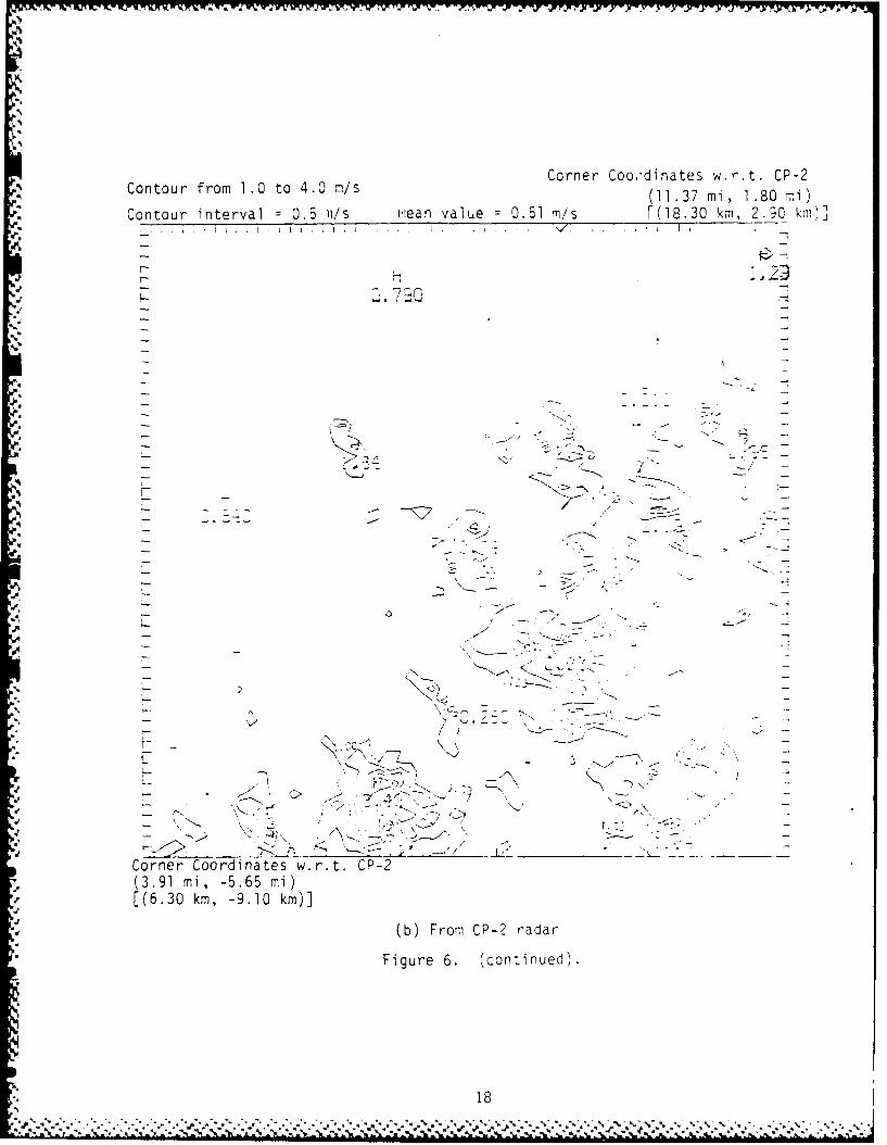
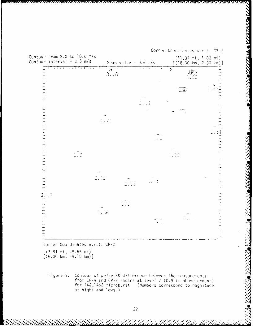
CP-2 and CP-4 radars, whose characteristics are listed in Table 2,simultaneously measured the turbulence information associated with the JAWSJuly 14 microburst. Since the two radars view the same turbulence fromdifferent directions (an angle of almost 90,), agreement between theirrespective measurements will indicate to what degree the microburst turbulencemay be considered isotropic. Figure 6 shows contours of the wind SD at aheight of 0.9 km from the CP-4 and CP-2 radars. Figure 7 shows contours ofthe absolute value of the wind SD difference between the CP-4 and CP-2 radars,Law = aw CP-4 - awCP-2! at a height of 0.9 km. Similar analysis for thepulse SD i's shown in Figures 8 and 9. The SD measurements from both CP-4 andCP-2 radars show good correlation with the exception of a few highly localizedlocations. These localized values cannot be described on a physical basis andare believed to be signal anomalies.
A cumulative probability technique has been used to quantitativelyillustrate the characteristics of the JAWS microburst turbulence measurements.Figure 10 shows the cumulative probability distributions of the pulse SD andthe wind SD for the 14JL1452 microburst measured with both the CP-2 and CP-"4radars. Figure 10 also shows the cumulative probability distributions of theSD differences, Law and Lap. These probabilities are derived from thefull-volume data set including 61 x 61 x 11 grid points. About 80 percent ofLap are less than 1 m/s, which is approximately equal to the backgroundturbulence level of the microburst, and 80 percent of Law are less than 0.5m/s. Therefore, it is concluded that the SD's from the CP-2 and CP-4 radarshave good correlation with each other in over 80 percent of the full volume.This correlation shows that both radars are measuring similar properties inthe same way and also suggests the turbulence to be isotropic. As expected,ao is larger than aw . This is because the second moment estimate involves adifference while the velocity estimate does not. Moreover, the second momentestimate is a better representation of turbulence intensity on a smaller scalecompared with the grid scales. Therefore, it is argued that the microburstturbulence intensity should be derived from the pulse SD by removing thespectral broadening effects mentioned earlier. A value of pulse SD in excessof 2.5 m/s exists for 50 percent of the full-volume data set. This suggeststhat over half of the microburst volume contains light to moderate turbulence.The wind SD, however, exceeds 2.5 m/s in less than I percent of the fullmicroburst volume. Finally, Figure 10 shows a limiting value of the spectrumwidth of about 1 m/s which represents the background turbulence levelthroughout the full microburst volume. This significant background value isattributed to the radial wind shear effects and was not found in any of threetornadic storms reported by Doviak and Zrnic' (1984). As it is clearly seen
14 0

Ip
' me
Corner Coordinates w.r.t. CP-2Contour from -10.0 to 10.0 m/s (30 *i -1.22 mi "
Contour interval = 1. r/s Acan value = -5.36m/s [(4.S K,. - 18.05 km)'
(4.3 mi -1 .- 7
- 05 k , 5 km)]--- V.-_-- -- .- -a. -
- 5. C of r i v 5 (1 m
above grou ) f r S 7 -. fLa
'a.,
_ / N- > - -/-. .
N -
- . N_ _ _/ "-
->-- --- --. . ",-_ ". . . ... ;
-- . _-. - -- -
.. ..... a..-
Corner Coordlinates w.r.t. CP-2(4.38 mi, -16.67 mi)[(-7.05 kin, -30.05 kin)]
(a) Radial ,velocity
Figure 5. Contour of radial velocity and pulse SD at level 5 (1 k~rmabove ground) for 5AUl847 inicroburst from CP-4. (Largenumbers correspond to magnitude of higns and lows woile -
smaller numbers represent contour values.)
i5
. -, .,a-,, . , ;, i ' , ,', , • , .4

Corner Coordinates .P.r.t. ?-2Contour from 3.0 to 9.5 m/s (3.03 m8 , -1122 '-,
Contour interval = 0.5 m/s Mean value 2.58 n/s [(4.95 kr, -12.05 k
KI
-7 7.--I 67 m
3- /0 . /! n
- -" 7 -d' 7, - -
_ " ~ . . . . . . ..J ... . -
,.
1 I/, , ,,
-,- q ki, - O O k - -.
Ni.e . (c n in e )
ieN
F.' . ",' .,, -"- ."- ."." " "" " :":"" ". "" . . ,"" ". ." • "" . - .""" - -""" - .""" - "-""". ."- . . . -'J- " "\""
. .'.- -,-.. .,' .' ,','., .. ..* .'-" . - , ' . '. ' 'i ., i ,,,' ., '. '. ', , ' / ,', . '.,. -.. .'..' .'. '.. ,' ,'- ',.-, . '.. .,,1 -* l ' " 1 m / ,

Corner Coordinates w.r.t. CP-2Contour froi 1.0 to 4.0 m/s (1.37 mi, 1.80 mi)
Contour interval = 0.5 m/s Mean value = 0.94 m/s [(18.30 kim, 2.90 km)]
z _0. G?00 . 1003 K-
-- -
4 '- - --
- ,>O ,/ -.'
7L-
__-._ _ "/ ,- _4K
-- :C - ',4KS,,,,s ,- -'-- /)' iN > \*
-- '"'- ', -" _ -
- ' "---I .S , ) -"
"
._ -'-'- \.< _. : , *, N -- , _ ..
.9 i - .6 "... , , " km, -- -1 km)
Figure K 6.Cnoro ind Da ee 09k bv rud o
--' ' K.. ' ,,. y 7_ ,
p.-," 7 I , -/ ,/ /" -
7-'7
• " "/" '..,,--2...-...-. -- • - -. - - - - ;"
Corner Coordinates w.r.t. CP-2
[(6.30 kin, -9.10 kin)]
(a) From CP-4 radar
Figure 6. Contour of wind SD at level 7 (0.9 km above ground) for14JL1452 microburst from CP-4 and CP-2. (Large numberscorrespond to magnitude of highs and lows while smallernumbers represent contour values.)
, I 7
.' .',"} - .,';','-',? ;.4 ;i - .- ,.-..,, :.., v ---.. -. ... , - -..- . .-. : -.-... . . .. ..-. : .-... < . : .,:; :17._"
h. -% - - TV .w IV
'i,
1,Corner Coordinates w.r.t. CP-2
Contour from 1.0 to 4.0 M/s (11.37 mi, 1.80 mi)
Contour interval = 0.5 ii/s mean value = 0.51 m/s [(18.30 kin, 2.90 kmr,
.p. .
;- L.4-
Cornr C.-o-i -
( . .- - - m-i . _
. +'1'.-..- -
-[ ( k , - 1 km- -
,Figur . (continu ).-
3 9m,1i
[(.0km 91 km)]
(b Fo C - raa
Figure 6.) (o tn e )
4. 1 8 '

Corner Coordinates w.r.t. CP-2Contour from 1.0 to 4.0 m/S (11.37 mi, 1.80 mi)Contour interval = 0.5 m/s Mean value = O.. m/s [(18.30 km, 2.90 km)]
- C. ,-,
-L tt I
-7
(3 9 mi -5 6-i
Figur 7. Cotu0.wn0D ifrne'ewentemaueet
ground fo 4L42_,rbrt.(ag umescre
spn tomgiud f .qh n o wwhlsm le
-~ 7
ConrCod n e s epresn CP vaue.
(3.9 mi
[(6.3.3 kin, -9.10 kin)],
Figure 7. Contour of wind SD differen e ',etween the measurementsfrom CP-4 and CP-2 radars at vel 7 (0.9 km aboveground) for 14JL1452 ricroburst. (Large numbers corre-spond to magnitude of highs and lows while smallernumbers represent contour values.,
19
• ._ b,.-, ,' %,_,[ -, -.-. ' - ' - . . .- *. -.. -.- . . , . . . .-.-.- ._ .•... _. . .. . . . . .. ,

PVI~fj"VARP-L-PWNr P6 AnRIVJlmlwrMnwmn M~n WI ul innPO WW0%nIV L-.WW~n ~-
Corner Coordinates w.r.t. CP-2
Con-'Iour from 3.0 to 10.0 rn/-- 11.37 mi, 1.80 mi)Contour in'L-2rval =0.5 m/s Mear value =2.5 ms [(18.30 kir, 2.90 kmn)]
(39 0i -565mi
[(. 3 km -9.1 km)
,,a)~~ Frm P- rda
Fiur 8 Cnturofpls S a lve 7(39kmabvegrun)=o14J 145 m cro ur t f om CP - an C -2 . (L rge nu ber'4
corrspon tomgiueo ihsadlw hl mle
numbers ~ *- rersn\otorvle.
-. ~20

.4.
Corner Cccrdinates w.r. U. CP-2
Contour from 3.0 to 10.0 m/s (11.37 mi, 1.30 mi)Contour interval = 0.5 m/s Mean value = 1.9 m/s L(18.30 kin, 2.90 kin)]
(3 9 mi_ -5 6 -iP63 km -91 k)
- ~~- • " )
4,,
'- 2 ,- 7" .
- _ -_ -- / .. --
- i ~~ ,/J.,-
-- .< --., --- _-3- -
- . _-a ,.Correr Coordinates w.r.t. CP-2
(3.91 mi, -5.65 mi)[(6.30 kin, -9.10 kin)] -
(b) From CP-2 radar
Figure 8. (continued).
21le
Corner Coordinates A.r.t. CP-,
Contour from 3.0 to 10.0 m/s (11.37 mi, 1.80 mi)Contour interval = 0.5 m/s Mean value = 0.6 m/s [(18.30 km, 2.90 km)]
-- , . -,-
-
:-44
Corner Coordinates w.r.t. CP-2
(3.91 mi, -5.65 mi)[(6.30 kiii, -9.10 km)]
7igure 9. Contour of pulse SO difference between the measurementsfrom CP-4 and CP-2 radars at level 7 (0.9 km above ground)for 14JL1452 microburst. (Numbers corresond to magnitude
of highs and lows.)
22
V2" - ' -' - - ' - '- - , -' -2-- - -, '- " " - '' '- - - - . , - .- '- - - , - - -" "

% ,~ -' ,~
A
F'
p
0
I -~C\J C'J SI.
I I0~
(-) C-, I 1 0*1 -~
o- ~ I K- 0
U
~ C\.~ C'j I p.~- I
a. o~ a. o. I I -~ Z\.C-) ~ C.~) C-) C-) C-)
-,
C- C-S... I
~ 3 Q-~A ~ -
I1 -'
I I ~ II I
~ I K -Hit ~.I -
/ -z A
/I I.I 1.:
DI. -, -.
I JigI -~ -
I It! -~ '4.-
/112 z :1.
I 2ft -~
/ I L/ (I/1 --/ I -~
I -~
// / -~
1'I,
/ *..,'I -~.1! 2 -~
//
f 5,
A?
24
M M- - ~ ~ d
S.
23

' S -o . . .. = - .
.
from Figure 11, the background turbulence intensity is significantly decreasedby the spectrum width broadening due to wind shear.
The spectrum width broadenings due to the radial wind shear, antennamotion, and the different fall speeds for various sized drops--as defined inEquations 5, 9, and 10 respectively--were evaluated and subtracted from thetotal spectrum width. In most situations, the broadening from both theantenna motion and the different fall speeds is small compared to that fromthe radial wind shear. The cumulative probabilities of the spectrum widthcontribution due to the radial wind shear, os , and the microburst turbulence,at are shown in Figure 11 for the 14JL1452 measurement from both the the CP-4and CP-2 radars. Microburst turbulence intensity, at, derived from the CP-4 1radar is consistent with that from the CP-2 radar over 80 percent of the fulfvolume. This, in turn, suggests that the microburst turbulence is essentiallyisotropic turbulence. It is interesting to note that the cumulativeprobability distribution of the wind SD, aw (see Figure 10), is very close tothat of the spectrum width broadening due to the radial wind shear shown inFigure 11.
Similar analyses are shown In Figures 12 and 13 for the 5AU1847 and30JN1823 microbursts, respectively. Among the three microbursts analyzed, theJAWS June 30 microburst contains the strongest turbulence, whereas the August5 microburst has the most complicated wind profile structure.
Finally, cumulative probabilities of the radial wind shear terms Kr, Ke,and K, as defined in Equation 6, for CP-4 and CP-2, are shown in Figures 14through 17 for the JAWS microbursts. It is seen that the microburst containslarger shear in the elevation direction than in the azimuthal direction. rnthe July 14 microburst, only 5 percent of all azimuthal shears are larger tlan5 x 10-J I/sec, while 35 percent of all elevational shears are in excess of 5x 10⁻³ 1/sec. In the August 5 case, 10 percent of the azimuthal shears arelarger than 10-2 1/sec and over 30 percent of the elevational shears arehigher than 10-2 1/sec. The radial velocity shear in the elevaticnaldirection of the JAWS microburst is larger than twice the values associatec "with the storms investigated by istok (1981). The difference is probably dueto the strong localized wind shear inherent in microburst storms which are amixture of an atmospheric boundary layer and downburst flow. An additionalexplanation is that Istok's grids are much coarser than JAWS data. Comparingthe wind shear terms shown in Figures 14 through 17, one can easily see thatthe August 5 microburst contains the strongest wind shear effects of the threemicrobursts analyzed. The August 5 microburst is, therefore, recommended as agood scenario for use in flight simulators for training avoidance ancoperational procedures if penetration Is unavoidable.
2.3 Comparison of Radar Data and Aircraft Data
A comparison between the turbulence intensities measured simultaneouslyby JAWS Doppler radar and aircraft has been made. Using a ground-based radarsystem and an instrumented aircraft, turbulence characteristics associatec(with thunderstorms at high altitudes (>3500 m above ground level) weredetected and studied by Burnham and Lee (1969), Lee (1977 and 1981), and Bohne(1981 and 1985). A comparison of some results from these previous studies
241
,. . . . ., . . .... . .
2S5~ *. . . - .. - . .- . . . .,.- -. . . . . . . . .

* - - -, - - - S - t S S
1%
*1I
Pu
/~* ~*'J C'.4 /
/ A~- ~- ~- o~ -~
I
'.- ~- ~-
C"-
C '1 -~
I ~ -~I -
I 'CD ~zj- U,
I .- 01 '4--
I *.CD -~,,' ~0 .-~
/ -n -~ 4-0
/ I: - -)I f:zo/ /.r) '4-
I 2 -~
I A S0Ii -~
1 /../ ,NJ
/ . 0-
/ . 0 _
/ .
/ // / -n
/f/I -)
/ C'~4
//
/ . Lfl
/ K..CD CD CD CD CD
CD CD
S pup
S
25 S
4-
.F~.A ,~4 J - .A .1 - ~ - .& -' - -S -P. J ~ ~ ~J ~

0
I Id
t CY
CD CD
UO I La 4-, 0 3j /P,
261

4 ~ - - S - . - .S-~ - - - - - .- . -,
-ft
.ft
A
I iii~I
ji: III: I --
/ _
3-. a
~0
- A
* -~ -4- 1'
* 0* .n
I . -
* 0 0
* ~ C)
I* I - -~
0I C)/ 0
I C).> ~-
// 0
3003/ 0S~ a
/I
aft
C)
u*. ft.
(~,/w) uOLWLA~C P~PPU~S
27 S
* * - * -. - ~ft** .-...

-a
t.
a-
4
0 .0 5 ,
0 . 04 .'%
K "7
0.03- / ...
,. . .........
N1
0.S 2 5 10 50 90 95 93 99.5
Cumulative Probability
Cigure 14. Cumulative probabilities of radial wi.id snear terms,
Kr, K , and K, for 14JL14b2 microburst for CP-4.
28 0
0.-J.

0.0~
/ K
0.0 2- 52 05 09 89.
Cumulative P.obabli itj
Figure 15. Cumulative probabilities of radial wind shear, terms,K, K', and Kfor 14JL1452 microburst for CP-2.
r9

... 0
K r
-.
K -0.05 2 059-5989.
-~ /
0.020
\
\
,), N N.... ---
0.5 2 5 10 50 90 95 98 99.5
Cumulative Probability(,.)
Figure 16. Cumulative probabilities of radial wind shear terms,* K,K, and K, for 5AU1847 microburst for C?-.
S.
30

0.1
0. 08 -
0.06
KI / -K
0.04/ -- O. 04K
/ / r/
0.02m
0 ... .. 5_ - L _ ... ..
0.5 2 5 10 50 90 95 98 99.5
Cumulative Probability (;)
Figure 17. Cumulative probabilities of radial wind shear terms, Kr,K, and K for 30JN1823 microburst for CP-4.
31
~ ~ -w - - -

with the current experimental measurements of microbursts at low altitudes(<2000 m above ground level) is made in this section.
During the JAWS field experiment, the NASA B-57B gust gradient aircraftwas used to measure turbulence along paths near microburst storms.Unfortunately, because of aircraft control restrictions during storms in theStapleton airport area, very few of these research aircraft flights coincidedwith the Doppler radar measurements. Table 3 shows the gust gradient flightsof the NASA B-57B aircraft during JAWS experiment. Among these flights, onlyRuns 23, 24, and 25 for Flight 6 coincide with Doppler data. These data weremeasured during the JAWS July 14 microburst. Figure 18 shows the relativepositions of the JAWS microburst and the aircraft flight paths for Runs 23,24, and 25. Run 24 was flown through the microburst almost simultaneouslywith the JAWS radar measurement. The run started at 14:50:50 MDT and lastedfor 87 seconds. Run 23 was flown through the field about 4 minutes earlierthan the JAWS measurment while Run 25 was flown approximately 2 minutes laterthan the radar scan and slightly outside of the microburst measurement volume.
Figures 19 and 20 depict the flight path information for Runs 24 and 23,respectively. Both runs are floin through the field at approximately 450 ft(150 m) above the ground. Figure 21 compares the total spectrum width, a,with the calculated turbulence intensities from Run 24 of the NASA B-57Bmeasurements. The plotted longitudinal, lateral, and vertical SD's from theaircraft data are relative to the body axis of the aircraft. The totalspectrum width (without subtracting any broadening) is about five times theturbulence intensity obtained from the aircraft. This agrees with thereported results of Robison and Konrad (1974) and Lhermitte (1968). Since theSD's from the aircraft measurements are relative to 2 to 3 second means, lowturbulence intensity values are expected.
As mentioned earlier, the JAWS microburst turbulence intensity, at, canbe calculated by subtracting the other spectrum width broadening effects fromthe total spectrum width. Comparison of the at with the calculated SD's fromthe NASA B-57B measurement is shown in Figure 22 for Run 24 and in Figure 23for Run 23. The wind standard deviation, aw, from the radar is also shown inthe figures. The aw is very consistent with the aircraft measurement.However, the microburst at is about three times that of the aircraft data. Acomparison between the turbulence intensities obtained from a NOAA/WPL lidarand the NASA B-57B aircraft was reported by Huang et al. (1985). One of theircomparisons is shown in Figure 24. The lidar spectrum width is again about 4to 5 times that of the aircraft-measured turbulence intensity. Bohne (1981)reported another comparison between a turbulence variance of a so-called"true" vertical gust velocity which was derived from an aircraft-measuredvertical gust velocity and a Doppler spectrum variance (shown in Figure 25).The turbulence variance of the "true" vertical gust velocity is relative tothe mean of the whole run. The correlation coefficient of these two variancesis 0.891.
Doppler radar and aircraft, of course, use different methods formeasuring turbulence information. The former measures turbulence contained ina full three-dimensional volume in space whereas the latter measuresinformation along the aircraft trajectory, i.e., a line in space. Thus,turbulence intensity meaured by the Doppler radar will, in general, be largeras shown in Figures 22 and 23. A better understanding of the relationship
32
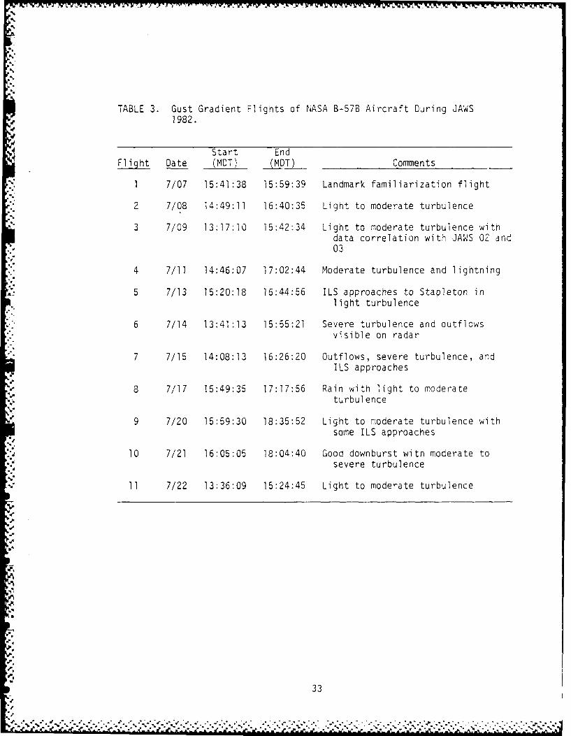
TABLE 3. Gust Gradient Flights of NASA B-57B Aircraft During JAWS
'1982.
Start EndFlight Date (MDT) (MDT) Comments
1 7/07 15:41:38 15:59:39 Landmark familiarization flight
2 7/08 14:49:11 16:40:35 Light to moderate turbulence
3 7/09 13:17:10 15:42:34 Light to moderate turbulence withdata correlation with JAWS 02 and03
4 7/11 14:46:07 17:02:44 Moderate turbulence and lightning
5 7/13 15:20:18 16:44:56 ILS approaches to Stapleton inlight turbulence
6 7/14 13:41:13 15:55:21 Severe turbulence and outflowsvisible on radar
7 7/15 14:08:13 16:26:20 Outflows, severe turbulence, andILS approaches
8 7/17 15:49:35 17:17:56 Rain with light to moderateturbulence
9 7/20 15:59:30 18:35:52 Light to moderate turbulence withsome ILS approaches
10 7/21 16:05:05 18:04:40 Good downburst with moderate tosevere turbulence
11 7/22 13:36:09 15:24:45 Light to moderate turbulence
33
. < . . - . . . . - - . . . ..5.'. . . - .. . . . -. . - .S. -. - .. . - . . - . , - . . . . - , . . . - . . . . . . .

40.2
An n 4July 14, 1982 ,
CP-
CP-4
39.7 ' ?-105.0 -104.5
Longitude (degrees) ''
Figure 18. Relative positions of 14jL145D2 microburst and flight --
paths of Runs 23, 24, and 25 in Flight 6 of NASA B-57Baircraft.
L 3
-J-
4 '

n~v I W. 0717 V Mm F O
P4
LO4
LL-J
4-3)
CU~
41 s- COCO 4
73
LA.n
Cl'C
ror
(5;p)~~~ CPl4~2 , j-
C C: C C
on c(1V- Iq6La
4.3 -*A..i-. -%

-- 7 - C.Jr
4- ......
I, I.-
~ -~, "L /
CD_ _ _ _ _ _ _ _I
-cr cn
(6p apnj je\
I-0 '1, -
S- co,- -
cm cm ' j j9~
-o zIS--
0 CD- )C
c)O r Ln
+J~ ~36

S.- S- -,
L
> --
+ CD- -
0
+ >
~~ >- CD ~
+ Ii
CDC + 2 C D
Lu IC3(2) "-
+ un0
+ 3h I
-4 . ..- + < ZI
4. CD-
+
++ W>. jj CD ~+ .. > Ll J--
++
4. - ~ C)
4.0 CCD 0 C C C) -
.N.
4..-..-
" " " .r ,- , ' .' " " ." . , '. . '. " ." .' ., . - , . ," - ' - '. " .' . , ' . . . r . - . - , • ' , - . . - ,.,L ..4.", . --. ", , . ,r , ,,",

71 CD -- - .
4-
+
+ +D 10 M.J
+~~ =A - f
+ -CDI -+-
+.
+ CD
4- C:) 0-V
+I -M -- = C
+' CEW
+ M4- CD -
4- ~ CD4- .C
+- J).,
+
4DC-C CD CDJ
CD D C CDCD rC;
(S/W) UO.LPLAaG PJPPUP13
38

.- >
-1 4- -. ,
13' -
+~EJ
-~ij
CD~.
-~ .4. .4-)
+ . . A,
+ !D
> 72
:P. .
+ N -iIQ C
+ ~ -j CDj
>I _j
+ -i >~ m )C
+ -jcrvC
> > 14J~:-'t >~ C
> 0u
1* > C)4.C 1 .
34.- > ~C)C3 C. C) 0
WY C)
. ... .
0Y
2530.
* -57B0 Lidar+ Recorded~Lidar
Z. O. - Spectral
-Width
-- 175 0.
-m.s o.. -_.
(a) Run 2
-; 250.
SOO
-to. __ . 2(b) Run 4
25S .E 1
-1 0. Ia . 0. Z. q(C) Run6
P. 1L V 1"'1 .b. ;
Figure 24. Comparison of radial mean wind velocity, calculated
turbulence intensity, and lidar spectral width betweenaircraft measurement and lidar measurement on February 7,
1984 (Huang and Frost 1934).
40

V) -Y
/ -J '.Z
/ -)
- -I
co 1. CD-
Oa/W @ULP
41G

between these two measurements is required in order to perfect a turbulencemodel to support the FAA and NCAR JAWS wind shear data sets. Also, thisunderstanding will be highly beneficial to the development of terminal Dopplerwind shear algorithms. More investigations, however, must be conducted tofully address this issue.
2.4 Microburst Turbulence Parameters
The important parameters for modeling turbulence are the turbulenceintensity, length scale, and spectrum. The Dryden spectrum is currentlyrecommended by the FAA AC-120-41 for wind shear turbulence modeling. Table 4shows the turbulence intensity and the turbulence length scale suggested i-this Advisory Circular for input to this spectrum. Both turbulence intensityand length scale are represented as a function of height only. In addition tothe height, turbulence parameters associated with a microburst should be afunction of the mean wind direction and the radial distance relative to themicroburst center. In this study, microburst turbulence is assumed to belocally isotropic, at least for the smaller scales of interest here but nothomogeneous on the large scale. Figure 26 schematically shows the top view ofa microburst. MC represents the center of the microburst; circles a, b, c,and d designate locations at different radial distances from the center; and1, 2, 3 ... A, B, C represent twelve directions emanating radially from themicroburst center. The arrows represent the quasi-steady mean wind directionat ground level for JAWS July 14, June 30, and August 5 microbursts,respectively. Coordinates of the three microburst centers relative to theCP-2 radar are listed in Table 5.
2.4.1 Turbulence Intensity
The profiles of at/V, which is the microburst turbulence intensitynormalized by the local quasi-steady mean wind, at four radial distances 4, 8,12, and 16 times the data set grid interval from the microburst center of theJuly 14 measurement are shown in Figure 27. Although the data are highlyscattered, a characteristic trend is discernible. To more clearly understandthis trend and to provide a functional relationship between the turbulenceintensity, at/V, radial distance from MC, and height above ground, a curve-fitting technique was applied.
The twelve directions given in Figure 26 were collected such as todivide the field into quarters. The directional dependence of the turbulenceintensity on the direction of the quasi-steady mean wind could then bestudied. The profile at/V in each quarter is then curve-fitted by the methodof least squares (see Figure 28). Comparison of the profiles at variousradial distances shows that the normalized turbulence intensity has highervariations along the mean wind direction (quarters, (3,4,5) and (9,A,B)) thanthe direction normal to the mean wind (quarters, (C,1,2) and (6,7,8)).
The Ct/V profiles at the various radial distances in a direction normalto the mean wind (quarters (C,1,2) and (6,7,8)) converge to a small value atradial distances greater than about four times the horizontal grid intervalfrom the MC. However, the at/V profiles in the upwind direction (quarter(3,4,5)) increases with radial distances especially at lower levels, and thenattains a maximum value at radial distance over 15 times the grid interval
42

.I
TABLE 4. FAA Turbulence Model in AC-120-41.
RMS Intensities Scale Lengths
Altitude (kts) (ft)
(feet)_ Long Lat Vert Long Lat Vert
20 3.40 2.70 2.34 105.7 49.7 10.4100 4.05 3.46 3.53 216.7 134.2' 53.0200 4.43 3.95 4.35 306.5 213.5 106.0400 4.85 4.50 5.36 433.5 339.6 212.0600 5.11 4.86 6.05 530.9 445.6 318.01500 5.74 5.78 7.94 840.9 824.5 795.3
= 2.33 z 0 . 1 2 L = 21.7 z0 . 5
= 1.56 z L = 4.2 z 0.73
0.2 0.8L 053 z1.0-_ = 0.98 z0 "2 8 V4 = 0.53 z '
TABLE 5. Center of JAWS Microbursts.
Coordinates ofMicroburst Center
w.r.t. CP-2
Data Sets (Mile) (Kin)
August 5, 1982 (-1.03, -14.94) (-1.65, -24.05)
June 30, 1982 (9.63, -11.18) (15.50, -18.00)
July 14, 1982 (8.76, -2.42) (14.10, -3.90)
43

. -. . . . . ..Y .-J W _7, - 7 7. .~. I V- I 1_ 0% 7
Mean Direction of Quasi-SteaJ, Windfor July 14 Microburst
4 3
6 2
Mean Direc: on of %au-Steady Wind for jneMicroburst '
8 C .
9 BA .
,',ean Direction of Quasi-Steady 'Windfor August 5 Microburst
Figure 26. Schermatic of sectors and radial lines relative to thericroburst center along which turbulence intensity wasevaluated.
44
. ..
..v * ., :riL

* , S ..I - ... - -- - - - - -
Y- N- -j wWT W r 717 2
,. - 2-
- - - _ E 2- -.: 7EH3
-" -- [ W,
-- . E
c. Radius 4 LX b. Radius 8 -X
=~ ql 6?~
Figure 27. Turbulence intensity t/V profiles at different radial
distances from the microburst center for the 14U'L1452microburst.
45
22 -Z-
C ~ .- -t2.1!, , .'- "-.',. "-.-.' ; k - -.-3-P .,,. . .-4% . . :-' '- 6 ' '. . -.-.. " ' - "; -" - " -" " -. "

9 0 C 0 1 .2 1 .0
e'o m- ..... 6.7.8 . -
7.0 u --.-- 9. A.B
7
a. .- Radius 4 , b .. Radiu S-,
0.0 1
I L
3.0 -. 0
0 .0
- a. Radius 4 -'X b. Radius 1 5 X
23 - -I 9..0 - -
. - " I +o F
5.0 "" ' .O -
¢. adus 2 X d Rdiu 1 H
Figure 28. Curve fit of the turbulence intensity profiles -tV
at different radial distances froIT the microburst
center for the 14JL1452 microburst.
46
3.0 ]

approximately at level 4 (750 m above the ground). Moreover, the Ct/V in thedownwind direction (quarter (9,A,B)) increases first at higher levels thenreaches a maximum value at radial distance about 12 times the grid interval ata level of approximately 9 (2000 m above the ground) and decreases at fartherradial distances from MC. At altitudes below 600 m, the upwind side ofturbulence is more severe than the downwind side of turbulence. However, thisis not true at higher altitudes (>600 m). These at/V profile characteristicssuggest that the microburst turbulence intensity is not only a function of theradial distance and height above the ground.but also depends on the directionof the quasi-steady mean wind. The August 5 and June 30 microbursts havesimilar at/V profiles but because the wind profile structure is much morecomplicated than the July 14 case whose quasi-steady wind field is quitesymmetric about the microburst center, the results obtained for at/V from theJuly 14 microburst are not completely the same for either the August 5 or June30 cases.
A functional form of the normalized at as a function of r, the radialdistance normalized by the horizontal grid interval, and h, the heightnormalized by the vertical grid interval, is written:
-r3 'T 0h
at(r,h) r2 h2
: A r h (11)
where
al bl cl di
a2 b2 c2 d2A =a 3 b3 c3 d3
a4 b4 c4 d4
where the elements of the matrix are determined by the curve-fittingtechnique. Table 6 lists the matrix elements for the 14JL1452 microburst.
2.4.2 Turbulence Length Scales
Length scale is another critical parameter for developing a turbulencemodel. The auto-correlation coefficient of the quasi-steady mean windcomponents along each radial direction shown in Figure 26 were curve-fit foreach level. Figures 29 and 30 are the three component auto-correlation curvesat three levels for the 14JL1452 and the 5AU1847 microbursts, respectively.The longitudinal component is in the direction of the horizontal mean wind.Based on the auto-correlation calculations, the integral length scales wereevaluated with the well-known relationship:
L = j R(x)dx (12)
0
47

TABLE 6. A Functional Form of Turbulence Intensity for 14JL1452Microburst.
ial1 bl Cl d 1, r3 T lh3
Zt r,h a a 2 b 2 c 2 d 2 r 2 h 2
a 3 b 3 c 3 d 3 IrI h
k.a 4 b4 c 4 d4j , ,
Quarter (C,1,2) (3,4,5) (6,7,8) (9,A,B)
a -0.551049E-06 0.741460E-05 0.911788E-06 0.657271E-06
b 0.407547E-05 -0.180272E-03 -0.246583E-04 0.334910E-05
c 0.197432E-03 0.102663E-02 0.104663E-03 -0.394346E-03
d -0.184692E-02 -0.130838E-02 -0.356118E-03 -0.268900E-03
a2 0332280E-05 -0.116770E-03 -0.270999E-04 -0.225209E-04
b 0.327677E-04 0.284746E-02 0.804118E-03 0.353051E-032
c2 -0.262014E-02 -0.163677E-01 -0.477002E-02 0.288334E-02
d2 0.229965E-01 0.241284E-01 0.824520E-02 0.266095E-02
a3 0.664155E-04 0.529400E-03 0.215985E-03 0.179236E-03
b3 -0.229589E-02 -0.132217E-01 -0.684668E-02 -0.457740E-02
c3 0,208904E-01 0.782930E-01 0.507962E-01 0189846E-01
d3 -0.569887E-01 -0.149245E+00 -0.642522E-01 -0.589026E-02
a4 -0.180032E-03 -0.704053E-03 -0.258038E-03 -0.130251E-03
b4 0.562896E-02 0.186553E-01 0.874772E-02 0.576422E-02
c4 -0.434284E-01 -0.962702E-01 -0.779505E-01 -0.458536E-01
d4 O.327257E+00 0.525894E+00 0.374366E+00 0.282357E+00
48
48I

Ground levelLevel #3(0.3 km above ground)
. . . Level #5(0.6 km above ground)
1.0
Longitudial component
0.0
-0.5
-1.0 , I I 1 I "0.0 2.0 4.0 6.0 8.0 10.0 12.0 14.0 16.0 18.0 20.0
_ 1 .0 ' I I i I I I
3o 0.5 Lateral component
C
2 0.0
. -0.5-10 0
0.0 2.0 4.0 6.0 8.0 10.0 12.0 14.0 . 1. 0 20.0
1 .0 II Iii
0.5 Vertical component0.5 - ",,
0.0 __
-0.5
-i.0 I n
0.0 2.0 4.0 6.0 8.0 10.0 12.0 14.0 16.0 18.0 20.0
Spatial Lag (1/200 m)
Figure 29. Auto-correlation coefficient of velocity components for14JL1452 microburst.
49
Sq

Oround 'evel-~~ - 31 3 '0.5 km above grcund)- -- - -. evel =5 (1.0 km abov'e ground)
1.0 1I
0.5 Longitudiali component
U. 0 .- - -- _ _
-0.5
3 !1.0 6.0 P.9 10.0 12.0 1/.0 lC.-, 12.0 20,.0
46-
S 0.5
; 0. G
01.
77 2.0 4.,D 6.0 8.0 10.0 12.0 1-1.1 16. C 1
1.0
0.5 Vert-Ical :,omponent
0.0,
-0.5
-i.00.0 2.0 4,.0 c.0 8.q 10.0 12.0 14.0 16.-D 18 .0 Z 0.0
Spatial Lag (1/150 m)
Figure 30. Auto-correlation coefficient of velocity components for5AU1847 microburst.
50

47WVVVM), V
Table 7 shows the integral scale at each level for the July 14 and August 5microbursts. As mentioned earlier, most investigators use a simple functionof height to model the turbulence length scale in the atmospheric boundarylayer. These functions are probably not true for microburst turbulence.Therefore, the relation between the turbulence scale and the height shown inTable 7 is used in the microburst turbulence simulation reported later in thisstudy. The magnitude of the turbulence length scales, however, is too largebecause they include scales larger than the grid size (150-200 m) of the JAWSdata sets. These scale sizes are already included in the quasi-steady winddata. To obtain a more representative length scale to use in the microburstturbulence simulation, the integral scales shown in Table 7 were somewhatarbitrarily multiplied by a constant factor of one-third to reduce them totypical grid sizes.
2.4.3 Turbulence Spectrum
In constructing a turbulence model, a key parameter is the spectrum ofthe turbulence. The spectrum is a measure of the energy associated withfluctuations of specific frequencies within the turbulence flow. The Ynormalized auto-spectra of the turbulence components measured in Flight 6 Runs24 and 23 of the NASA B-57B aircraft program are shown in Figures 31 and 32.The corresponding analytical Dryden and von Karman spectrum models are alsoshown in the figures. It can be seen that both the Dryden and von Karmanspectra are reasonable approximations to the turbulence spectra measured nearthe microburst. Thus, since the two models appear to give similar results andbecause the form of the Dryden spectrum is more readily adaptable tomathematical manipulation, it is used in this study. Also, the Drydenspectrum is the spectrum currently recommended by the FAA in AC-120-41. TheDryden spectra for the three velocity fluctuation components, respectively,can be written as:
2A1
1 + A12K2
A2 I + 3 A22K2
=2K 02 2- (13)2 (1 + A22K2)2
= 1 + 3 A32K2
-(I + A3 2K2)2 ]
where the subscripts 1, 2, and 3 represent the longitudinal, lateral, andvertical components, respectively; A is the length scale; a is the turbulenceintensity; and K is the wave number.
51

TABLE 7. Integral Scales.
August 5, 1982, 1847 Microburst
Longitudinal Lateral VerticalLevel (m) (M) (M)
1 (0 m) 319 513 0
2 (250 m) 419 450 355
3 (500 m) 464 666 351
4 (750 m) 559 682 338
5 (1000 M) 520 713 317
6 (1250 m) 403 473 292
7 (1500 m) 473 334 254
8 (1750 m) 468 475 234
9 (2000 m) 524 521 236
July 14, 1982, 1452 Microburst
Longitudinal Lateral VerticalLevel (M) (M) (M)
1 (0 m) 422 422 0
2 (150 m) 558 336 292
3 (300 m) 465 432 310
4 (450 m) 549 515 338
5 (600 m) 553 421 369
6 (750 m) 526 427 391
7 (900 m) 433 435 395
8 (1050 M) 437 417 385
9 (1200 m) 365 409 374
10 (1350 m) 456 577 367
11 (1500 m) 418 500 367
52 0
*** ~ ~ **' ~ ** ~ .. S. .. .2

kk
von Karman - - rden ;'J*6
TL 805 m TL= 840 m TL =821 m
N= 5S1Z N: 512 FNZ 3,2lo- ECG.= 6 SE:= SEC.: 6
... WXL WxC WX%
100
-J~S S
rz
T'L = 6?9 m TL = 516 m TL 6 09 ltNSZ F N= $1Z N= 512' SEG.= .- SEC. =S SEG.: ,6
l -r
SN1=N
SEC.=. 5 E.
o F"
II X -A -..10-S10 - 2 ion 10-8 IO 10-2 ~
Ic = /v (M-')
Figure 31. lormalized auto-spectra of turbulence components (Flight 6,Run 24; NASA B-57B aircraft).
53
. , ,. - "- S. -. '_-.,.." . . . ... . ."-" "' . -V

von Karman Dryden
TL 807 m TL = 799 m TL = 776 m
102 _ N=1021 N=11024 N=102S= 7EG.= 7
b FWXL VXC WXR
10-i
TL = 1888 m TL = 1868 m TL = 1912 m10 N=102 N=1024 N=1024
1 2SEG. = 7 SEG. = 7 SE . = 7WYL + wyc WYL
+ +Y
~10Or.0
LL4 -
TL =384 m TL= 511 m TL =406 m
i0 z N=1024 N: 102.
N= 1024S -5E.EG. 7
_7 U- Zc W ZR
100
4 10-
10 - 2 I0° 10-2 Ica 10 - 2 I0
°
IC = /v (ni-')
Figure 32. Normalized auto-spectra of turbulence components (Flight 6,
Run'23; NASA B-57B aircraft).
54
,]

3.0 MICROBURST TURBULENCE MODEL AND ITS APPLICATIONIN FLIGHT SIMULATION
The microburst turbulence intensity and length scale obtained in theprevious sections, although somewhat subjective and based on limited data,were used to develop a microburst turbulence simulation model. Az-transformation technique, which is based on the Dryden hypothesis of thespectral density function of turbulence and Taylor's frozen eddy hypothesis,has been developed by Wang and Frost (1980) and Huang and Frost (1984). Weassume that the Isotropic shapes of the spectrum hold for the non-isotropicconditions which occur at a very low altitude but that the turbulenceintensity and the integral scale vary spatially.
Microburst turbulence components along an aircraft's trajectory arecalculated by utilizing the z-transform technique. This technique uses afilter function, namely, the Dryden spectrum. Gaussian white noise signalsare computer generated and passed through the filter to provide the simulatedtime history of the turbulence as output (see Figure 33). The same techniqueis also applied to generate the turbulence model suggested by the FAA inAC-120-41, and the two models are compared in a later section.
Using a rational spectral model, simulated turbulence can be generatedwith the difference equations. The z-transformation technique is a digitalsimulation model where the nth turbulent point is a function of the previousturbulence fluctuation values and noise signals. For the Dryden model, thedifference equations are written as (see Huang and Frost 1984):
Yn = ClYn-1 + C2Yn-2 + diXn-1 + d2xn-2 (14)
where ci, c2 , dl, and d2 are parameters depending on the sampling rate (st),mean wind speed (V), turbulence intensity (ai, 02, and a3), and turbulencelength scale (XI, X2, and X3 ); y represents the digital generated turbulencecomponent; and x designates the digital random noise signal. For the Drydenmodel, the constant parameters ci, c2 , dl, and d2 are given as:
3
0'
G3u-sian Filter SimulatedWhite Noise Atmospheric
Turbulence
Figure 33. Turbulence si; ulation technique.
55

cI = exp Y At)
c2 0 (15)
dX I d, =01 ~j (-cl)
AtV
d2 =0
for the longitudinal component and
cl 2exp f 2 At
c2 -exp -2 V At (16)X2 j
3Vd 22 ' 2 1 1A X2
V-1 /-I VJJ
d2 2 f 21 -t _
d 0L2 3 V I3
for the lateral component. The vertical component has the same form as thelateral component, except for a different length scale and turbulentintensity, i.e., X3 and c3. The sampling interval used in the simulation is0.5 second.
Results of the simulation are presented in Figures 34 through 37 usingthe FWG/JAWS and the FAA turbulence models, respectively. Figures 34 and 35show three typical turbulent wind velocity components (quasi-steady mean wind+ turbulence fluctuation) and resulting trajectories of a B727-type aircraftapproaching through the JAWS 5AU1847 microburst along path AB (zo = 300 ft).The nomenclature used in defining the orientation of the runway to the windfield for both approach and takeoff cases are those described in Frost et al.(1985) (see Appendix). The simulation in Figure 34 uses the turbulence modelderived from the JAWS data; Figure 35 shows similar results using theturbulence model suggested by the FAA in AC-120-41. While microburstturbulence may increase the workload of a pilot, its influence on theaircraft's trajectory would not, in general, be significant enough to alterthe outcome of an approach or take off. Figures 36 and 37 show the spatialhistory of the turbulence fluctuations encountered by the aircraft in thesimulation results given in Figures 34 and 35, respectively. Since the samenoise signals are used for both the FWG/JAWS and the FAA models, the
56
ILS

pa,
5'a
C) C: C C J__ c- a
C:) 10 C~i oc -J
I) PU L20 LJ.A G
(sl~l) PULMA
C) C_ C"D(14) lq6 @H A
C~j 'a.
1 PU ~j O. I P
ko --el

VN 3
I
S UL
-p 58

~~V '~ jw~~ ~ V ~ W XwY~cW~U~WiW 'r ~ w~..l
4-'
CDA
LL)U~p; 6uo
(sj sq~uodoo ~u@Lqjn
559
If..

Lfl
Ln.
CUA
z
C)
LPL;D :\.le LQUpnj u
Ap-~~~ . . . . . .
It-

turbulence fluctuation patterns encountered by the aircraft are roughlysimilar to each other. However, the figures do show that the aircraftencounters more severe turbulence with the JAWS model than with the FAA model,especially near the microburst center. This increased turbulence in theregion of strong shear is very consistent with physical reasoning and suggeststhat the JAWS model is physically more realistic.
Finally, a number of takeoffs with turbulence superimposed weresimulated. Turbulence effects on the aircraft were assumed negligible untilthe aircraft's liftoff. Results of five takeoffs for different turbulencerealizations based on the FWG/JAWS model (5AU1847 microburst) along theintended path AB (z0 = 66 ft) are presented in Figure 38. Total turbulentvelocity components (quasi-steady mean wind + turbulence fluctuations) and theaircraft's trajectories in a vertical plane are shown in the figure. Based onthese five simulations, the maximum deviation of the climb-out trajectory fromthe reference flight path computed without turbulence is approximately 80 ftat a horizontal distance about 2 nautical miles from brake release. Thestandard deviations of the aircraft trajectories about the no turbulenceflight path at horizontal distances of 1.5, 2.0, and 2.5 nautical miles are25, 45, and 50 ft, respectively. Turbulence effects clearly influence theclimb-out trajectory; however, this influence on the ultimate outcome of thedeparture is not, in general, significant. This conclusion is also true forthe landing simulations shown earlier. However, in those cases, maximumdeparture from the intended flight path was on the order of 250 to 300 ft.
61
::2

%~~:: .- 7-.
CD C D C D C DC
p.J U ' P)LJ A SI P LP @H( q LH0
CD CD C
PULM LP~a2 L
62-

4.0 CONCLUSIONS
Turbulence information associated with the JAWS microburst data setsmeasured on August 5, July 14, and June 30, 1982, has been analyzed.Microburst turbulence intensity is calculated by subtracting the spectrumbroadenings due to wind shear, antenna motion, and precipitation fall speedsfrom the second moment, namely, the radar spectral width. (Note that thepulse volume was a Cressman weighted average as discussed in Section 2.1.)The analysis shows that local isotropic turbulence is a reasonable assumptionfor the microburst turbulence model. The August 5 microburst, recommended asa good scenarios to be used in flight simulations, contains the strongest windshear and most significant turbulence effects among the three micrcbursts.Both the von Karman and Dryden analytical spectrum functions appear to be gocdapproximations of the partitioning of energy among the turbulent eddies (atleast for high frequency) in a microburst.
Comparison of the turbulence intensity derived from the JAWS radarsecond moment with that from the in situ measurement of the NASA B-57Baircraft shows the former is about three times of the latter. This differenceis probably caused by the fact that the radar-measured turbulence intensity isrepresentative of three-dimensional spatially distributed turbulence and theaircraft-measured value is based on the aircraft's trajectory only. Severalinvestigators reported a similar inconsistency between the radar/lidarspectral width which is regarded as a turbulence indicator and theaircraft-measured turbulence intensity. Efforts to examine this areatheoretically and experimentally are highly recommended.
A z-transformation turbulence simulation technique has been developed toaccount for small-scale perturbation not previously contained in the smoothedJAWS mlcroburst quasi-steady wind profiles (JAWS microburst data sets). Theturbulence model derived from the radar-measured turbulence information isbelieved to be physically more realistic than the FAA AC-120-41 model becauseit shows stronger turbulence intensity in the high shear regions of themicroburst. Flight simulations of a B727-type aircraft through the JAWSmicrobursts with turbulence superimposed suggest that although workload of apilot may be significantly increased, the outcome of the approach or takeoffis, in general, not changed.
63,-0,
................--- °-g°

REFERENCES
Barr, N. M., D. Gangaas, and 0. R. Schaeffer (1974). "Wind Models for FlightSimulation Certification of Landing and Approach Guidance and ControlSystems," FAA Report No. FAA-RD-74-206.
Bohne, A. R. (1985). "Joint Agency Turbulence Experiment--Final Report,"AFGL-TR-85-0012, January.
Bohne, A. R. (1981). "Radar Detection of Turbulence in Thunderstorms,'AFGL-TR-81-0102, March.
Boldman, 0. R., and P. F. Brinich (1977). "Mean Velocity, TurbulenceIntensity, and Scale in a Subsonic Turbulent Jet Impinging Normal to aLarge Flat Plate," NASA TP-1037.
Burnham, J., and J. T. Lee (1969). "Thunderstorm Turbulence and ItsRelationship to Weather Radar Echoes," Journal of Aircraft, 6(5),Sept.-Oct.
Campbell, W. C. (1984). "A Spatial Model of Wind Shear and Turbulence forFlight Simulations," NASA TP-2313, May.
Costello, F. A. (1976). "Velocity Field of a Gaussian Circular Jet withNormal Impingement," Journal of Applied Mechanics, Dec., pp. 551-554.
Crabb, D., D. F. G. Durao, and J. H. Whitelaw (1981). "A Round Jet Normal toa Crossflow," Journal of Fluids Engineering, 103:142-153, March.
Doviak, R. J., and 0. S. Zrnic' (1984). "Doppler Radar and Weather
Observation," Academic, Orlando, Fla.
Elmore, K. L., and J. McCarthy (1984). Private communication.
Fichtl, G. H. (1973). "Problems in the Simulation of AtmosphericBoundary-Layer Flows," AGARD Conference Proceedings No. 140, AdvisoryGroup for Aerospace R&D, Neuilly Sur Sein, France.
Frost, W. (1984). "Turbulence Models," Presentation at the NASA Langley WindShear/Turbulence Workshop, May 30-June 1.
Frost, W., and R. Bowles (1984). "Wind Shear/Turbulence Inputs to FlightSimulation and Systems Certification," Proceedings. NASA LangleyResearch Center, Hampton, Va.
Frost, W., H. P. Chang, K. L. Elmore, and J. McCarthy (1985). "MicroburstWind Shear Models from JAWS," Final report under NCAR Subcontract S3011,January.
Frost, W., R. E. Turner, and B. H. Long (1978). "Engineering Handbook on theAtmospheric Environmental Guidelines for Use in Wind Turbine GeneratorDevelopment," NASA TP 1359.
64
; ' ".- ..-. '?:'-...,.- .. . . . .. . . . . .....- , .. ,.-.... " ........ ... .. ., . -..-... .-

7 . - - .V. V -r;- _d %
Huang, K. H., and W. Frost (1984). "Monte Carlo Particle Dispersion (MoCaPD)Model of Battlefield Obscuration," Final report for US Army ContractOAAG29-81-D-0100, by FWG Associates, Inc.
Istok, M. (1981). "Analysis of Doppler Spectrum Broadening Mechanisms inThunderstorms," Paper presented at the 20th Radar MeteorologyConference.
Keeler, J., and C. Frush (1985). Private communication.
Lee, J. T. (1981). "Doppler Radar-Research and Application to Aviation FlightSafety, 1977-1979," DOT/FAA/RD-81/79, June.
Lee, J. T. (1977). "Application of Doppler Weather Radar to TurbulenceMeasurements Which Affect Aircraft," FAA-RD-77-145, 44 pp.
Lhermitte, R. M. (1968). "Turbulent Air Motions as Observed by DopplerRadar," Preprints of the 13th Radar Meteorology Conference, Montreal,Canada. American Met. Society, Boston, Mass.
Robison, F. L., and T. G. Konrad (1974). "A Comparison of the TurbulentFluctuations in Clear Air Convection Measured Simultaneously by Aircraftand Doppler Radar," Journal of Applied Meteoroloay, 13:481-487.
Shayesteh, M. V., I. M. M. A. Shabaka, and P. Bradshaw (1985). "TurbulenceStructure of a Three Dimensional Impinging Jet in a Cross Stream,"AIAA-85-0044, AIAA 23rd Aerospace Sciences Meeting, Jan. 14-17, Reno,Nev.
Wang, S. T., and W. Frost (1980). "Atmospheric Turbulence SimulationTechniques with Application to Flight Analysis," NASA CR-3309.
Zegadi, R., J. L. Balint, R. Morel, and G. Charnay (1983). "The Influence ofa Low Reynolds Number on an Impinging Round Jet," Structure of ComDlexTurbulent Shear Flow, IUTAM Symposium Marseille 1982 (R. Dumas and L.Fulachier, eds.).
65
,.-.-. .,, -.-... . . - . . . .- .-. - . -- --- .... ..... ..

APPENDIX
NOMENCLATURE USED IN APPROACH/TAKEOFF SIMULATIONS
The nomenclature used in defining the orientation of the runway to thewind field are illustrated in this Appendix for both approach and takeoffcases. To investigate the influence of the microburst position relative tothe intended touchdown or liftoff point on the runway, the center of themicroburst is mathematically shifted along the path with respect to therunway. The runway is positioned relative to the center of the microburstsuch that an aircraft following the glide slope or takeoff path passes throughthe center of the microburst at a given height to be designated as zo .
Figure A.1 schematically depicts the nomenclature used in the approachsimulations. The intended touchdown point, TD, is the threshold of the runwaycorresponding to the specific flight path. The distance of the threshold fromthe microburst center is calculated as zo/tan y, where y is the glide slopeangle. A value of zo = 0 corresponds to the threshold of the runwaycoinciding with the microburst center. The orientation of the runway, 9, ismeasured relative to the positive x direction. The (xo,yo) coordinatesdesignate the position in the horizontal plane at which zo is measured.Values of xo and yo are measured relative to an origin located at thenorthwest corner of the full-volume data set. For the August 5 microburst,the origin is at (-4.38 mi, -11.22 mi), (-7.05 km, -18.05 km), as measuredfrom CP-2.
Takeoff path definition and orientation are shown in Figure A.2. Theliftoff point, LO, is the end of the runway corresponding to the specificflight path. A 10° liftoff path with 5000 ft ground run (see Figure A.2) isselected as a refernce only for purposes of defining the position of themicroburst relative to the runway. The B727-type aircraft, for example, wouldliftoff after approximately a 5000 ft run but would climb-out on anapproximate 6.4° path if there was zero wind. The location of the center ofthe microburst is selected relative to the liftoff point, in a manner similarto that of the approach. The value of zo for takeoff is defined as the heightat which the aircraft would pass through the center of the microburst whenaccelerating along the runway for 5000 ft and then climbing out along anarbitrarily defined 10° reference path. A negative zo indicates the aircraftis passing through the center of the microburst while still on the runway.
66
,!
I. ~ * . -!

S-~ -::-LLx C'4j C)
0~ C:) ON
0 CD
L P/4
00
41-) C
o CD
~ I
CL CD
(..

*~j I!w *.. - Q -- 4 4 - -
U')'
E v0 - -O
4- %
I 4-J
00 t4--41)
00
4-) J
4-.
N-zi
LU L
co CDJ
LUL
N.E -14
OC- Lfl c
=6

ThR1~
-. .....-..
-~ - .-w
w S S S S S 0 0 S S S S S


