A Non-Convex Relaxation for Fixed-Rank Approximation

Carl Olsson1,2 Marcus Carlsson2 Erik Bylow2

1Department of Electrical EngineeringChalmers University of Technology

2Centre for Mathematical SciencesLund University

Abstract

This paper considers the problem of finding a low rankmatrix from observations of linear combinations of its el-ements. It is well known that if the problem fulfills a re-stricted isometry property (RIP), convex relaxations usingthe nuclear norm typically work well and come with theo-retical performance guarantees. On the other hand theseformulations suffer from a shrinking bias that can severelydegrade the solution in the presence of noise.

In this theoretical paper we study an alternative non-convex relaxation that in contrast to the nuclear norm doesnot penalize the leading singular values and thereby avoidsthis bias. We show that despite its non-convexity the pro-posed formulation will in many cases have a single station-ary point if a RIP holds. Our numerical tests show that ourapproach typically converges to a better solution than nu-clear norm based alternatives even in cases when the RIPdoes not hold. 1

1. IntroductionLow rank approximation is an important tool in appli-

cations such as rigid and non rigid structure from motion,photometric stereo and optical flow [30, 5, 31, 14, 2, 13].The rank of the approximating matrix typically describesthe complexity of the solution. For example, in non-rigidstructure from motion the rank measures the number of ba-sis elements needed to describe the point motions [5]. Un-der the assumption of Gaussian noise the objective is typi-cally to solve

minrank(X)≤r

‖X −X0‖2F , (1)

where X0 is a measurement matrix and ‖ · ‖F is the Frobe-nius norm. The problem can be solved optimally using SVD[10], but the strategy is limited to problems where all matrix

1This work has been funded by the Swedish Research Council (grantsno. 2012-4213 and 2016-04445) and the Swedish Foundation for StrategicResearch (Semantic Mapping and Visual Navigation for Smart Robots).

elements are directly measured. In this paper we will con-sider low rank approximation problems where linear com-binations of the elements are observed. We aim to solveproblems of the form

minX

I( rank(X) ≤ r) + ‖AX − b‖2. (2)

Here I( rank(X) ≤ r) is 0 if rank(X) ≤ r and ∞ other-wise. The linear operator A : Rm×n → Rp is assumed tofulfill a restricted isometry property (RIP) [29]

(1− δq)‖X‖2F ≤ ‖AX‖2 ≤ (1 + δq)‖X‖2F , (3)

for all matrices with rank(X) ≤ q. The standard approachfor problems of this class is to replace the rank functionwith the convex nuclear norm ‖X‖∗ =

∑i xi, where xi,

i = 1, ..., N are the singular values of X , [29, 6]. It wasfirst observed that this is the convex envelope of the rankfunction over the set {X;x1 ≤ 1} in [12]. Since then anumber of generalizations that give performance guaran-tees for the nuclear norm relaxation have appeared, e.g.[29, 27, 6, 7]. The approach does however suffer from ashrinking bias that can severely degrade the solution in thepresence of noise. In contrast to the rank constraint the nu-clear norm penalizes both small singular values of X , as-sumed to stem from measurement noise, and large singu-lar values, assumed to make up the true signal, equally. Insome sense the suppression of noise also requires an equalsuppression of signal. Non-convex alternatives have beenshown to improve performance [26, 23, 19, 24].

In this paper we will consider the relaxation

minXRr(X) + ‖AX − b‖2, (4)

where

Rr(X) = maxZ

N∑i=r+1

z2i − ‖X − Z‖2F , (5)

and zi, i = 1, ..., N are the singular values of Z. The min-imization over Z does not have any closed form solution,however it was shown in [21, 1] how to efficiently evaluate

1

and compute its proximal operator. Figure 1 shows a threedimensional illustration of the level sets of the regularizer.In [21, 20] it was shown that

Figure 1: Level set surfaces {X | Rr(X) = α} for X =diag(x1, x2, x3) with r = 1 (Left) and r = 2 (Middle).

Note that when r = 1 the regularizer promotes solutionswhere only one of xk is non-zero. For r = 2 the regu-larlizer instead favors solutions with two non-zero xk. Forcomparison we also include the nuclear norm. (Right)

Rr(X) + ‖X −X0‖2F , (6)

is the the convex envelope of

I( rank(X) ≤ r) + ‖X −X0‖2F . (7)

By itself the regularization term Rr(X) is not convex, butwhen adding a quadratic term ‖X‖2F the result is convex. Itis shown in [1] that (7) and (6) have the same optimizer aslong as the singular values of X0 are distinct. (When this isnot the case the minimizer is not unique.) Assuming that (3)holds ‖AX‖2 will behave roughly like ‖X‖F for matricesof rank less than q, and therefore it seems reasonable that(4) should have some convexity properties. In this paper westudy the stationary points of (4). We show that if a RIPproperty holds it is in many cases possible to guarantee thatany stationary point of (4) (with rank r) is unique.

A number of recent works propose to use the related‖ · ‖r∗-norm [22, 11, 18, 17] (sometimes referred to as thespectral k-support norm). This is a generalization of the nu-clear norm which is obtained when selecting r = 1. It canbe shown [22] that the extreme points of the unit ball withthis norm are rank r matrices. Therefore this choice maybe more appropriate than the nuclear norm when search-ing for solutions of a particular (known) rank. It can beseen (e.g. from the derivations in [18]) that ‖X‖r∗ isthe convex envelope of (7) when X0 = 0, which gives‖X‖2r∗ = Rr(X) + ‖X‖2F . While the approach is convexthe extra norm penalty adds a (usually) unwanted shrinkingbias similar to what the nuclear norm does. In contrast, ourapproach avoids this bias since it uses a non-convex regu-larizer. Despite this non-convexity we are still able to derivestrong optimality guarantees for an important class of prob-lem instances.

1.1. Main Results and Contributions

Our main result, Theorem 2.4, shows that if Xs is a sta-tionary point of (4) and the singular values zi of the matrixZ = (I − A∗A)Xs + A∗b fulfill zr+1 < (1 − 2δ2r)zrthen there can not be any other stationary point with rankless than or equal to r. The matrix Z is related to the gra-dient of the objective function at Xs (see Section 2). Theterm ‖X − Z‖2 can be seen as a local approximation of‖AX − b‖2 =

‖X‖2F − 〈X, (I −A∗A)X〉 − 2〈X,A∗b〉+ bTb. (8)

Replacing 〈X, (I −A∗A)X〉 with its first order Taylor ex-pansion 2〈X, (I − A∗A)Xs〉 (ignoring the constant term)reduces (8) to ‖X − Z‖2 + C, where C is a constant.

If for example there is a rank r matrix X0 such thatb = AX0 then it is easy to show that X0 is a stationarypoint and the corresponding Z is identical to X0. Since thismeans that zr+1 = 0 our results certify that this is the onlystationary point to the problem ifA fulfills (3) with δ2r < 1

2 .The following lemma clarifies the connection between thestationary point Xs and Z.

Lemma 1.1. The point Xs is stationary in F (X) =Rr(X) + ‖AX − b‖2 if and only if 2Z ∈ ∂G(Xs), whereG(X) = Rr(X) + ‖X‖2F , and if and only if

Xs ∈ argminX

Rr(X) + ‖X − Z‖2F . (9)

(The proof is identical to that of Lemma 3.1 in [25].) In[1] it is shown that as long as zr 6= zr+1 the unique solutionof (9) is the best rank r approximation of Z. When thereare several singular values that are equal to zr, (9) will havemultiple solutions and some of them will not be of rank r.Note however, that since (9) is the convex envelope of (7)(with X0 = Z) the solution set of (9) is the convex hull ofthat of (7), and therefore there are still solutions of rank r to(9) even when zr = zr+1.

Stationary points of F will therefore generally be rankr approximations of Z. In this situation the first r singularvalues of Z coincide with those of X while the remainingones are related to the residual error. Hence, loosely speak-ing our results state that if the error residuals are small com-pared to Xs this stationary point is likely to be unique.

Our work builds on that of [25] which derives similarresults for the non-convex regularizer Rµ(X) =

∑i µ −

max(√µ − xi)

2, where xi are the singular values of X .In this case a trade-off between rank and residual error isoptimized using the formulation

minXRµ(X) + ‖AX − b‖2. (10)

While it can be argued that (10) and (4) are essentiallyequivalent since we can iteratively search for a µ that gives

the desired rank, the results of [25] may not rule out the ex-istence of multiple high rank stationary points. In contrast,when using (4) our results imply that if zr+1 < (1−2δ2r)zrthen Xs is the unique stationary point of the problem. (Tosee this, note that if there are other stationary points we canby the preceding discussion assume that at least one is ofrank r or less which contradicts our main result in Theo-rem 2.4). Hence, in this sense our results are stronger thanthose of [25] and allow for directly searching for a matrix ofthe desired rank with an essentially parameter free formula-tion.

In [8] the relationship between minimizers of (4) and (2)is studied. Among other things [8] shows that if ‖A‖ ≤ 1then any local minimizer of (4) is also a local minimizerof (2), and that their global minimizers coincide. Henceresults about the stationary points of (4) are also relevant tothe original objective (2).

Some very recent papers [4, 28, 15] parametrize X us-ing UV T , where both U and V have r columns. Theyshow that it is possible to bound the distance between theglobal and any local minimum in terms of the residual error‖A(UV T )−b‖2 if a RIP holds. In contrast to our results thisdoes however not rule out the existence of multiple minima(except in the noise free case).

1.2. Notation

In this section we introduce some preliminary materialand notation. In general we will use boldface to denote avector x and its ith element xi. Unless otherwise stated thesingular values of a matrix X will be denoted xi and thevector of singular values x. By ‖x‖ we denote the stan-dard euclidean norm ‖x‖ =

√xTx. A diagonal matrix

with diagonal elements x will be denoted Dx. For matri-ces we define the scalar product as 〈X,Y 〉 = tr(XTY ),where tr is the trace function, and the Frobenius norm‖X‖F =

√〈X,X〉 =

√∑ni=1 x

2i . The adjoint of the lin-

ear matrix operator A is denoted A∗. By ∂F (X) we meanthe set of subgradients of the function F at X and by a sta-tionary point we mean a solution to 0 ∈ ∂F (X).

2. Optimality ConditionsLet F (X) = Rr(X)+‖AX−b‖2. We can equivalently

write

F (X) = G(X)− δq‖X‖2F +H(X) + ‖b‖2, (11)

where G(X) = Rr(X) + ‖X‖2F and H(X) = δq‖X‖2F +(‖AX‖2 − ‖X‖22

)− 2〈AX,b〉. The function G is convex

and sub-differentiable. Any stationary point Xs of F there-fore has to fulfill

2δqXs −∇H(Xs) ∈ ∂G(Xs). (12)

Computation of the gradient gives the optimality conditions2Z ∈ ∂G(Xs) where Z = (I −A∗A)Xs +A∗b.

2.1. Subgradients of G

For our analysis we need to determine the subdifferen-tial ∂G(X) of the function G(X). Let x be the vector ofsingular values of X and X = UDxV

T be the SVD. UsingVon Neumann’s trace theorem it is easy to see [21] that theZ that maximizes (5) has to be of the form Z = UDzV

T ,where z are singular values. If we let

L(X,Z) = −r∑i=1

z2i + 2〈Z,X〉, (13)

then we have G(X) = maxZ L(X,Z). The function L islinear in X and concave in Z. Furthermore for any given Xthe corresponding maximizers can be restricted to a com-pact set (because of the dominating quadratic term). ByDanskin’s Theorem, see [3], the subgradients of G are thengiven by

∂G(X) = convhull{∇XL(X,Z), Z ∈ Z(X)}, (14)

where Z(X) = argmaxZ L(X,Z). We note that byconcavity the maximizing set Z(X) is convex. Since∇XL(X,Z) = 2Z we get

∂G(X) = 2 argmaxZ

L(X,Z). (15)

To find the set of subgradients we thus need to determineall maximizers of L. Since the maximizing Z has the sameU and V as X what remains is to determine the singularvalues of Z. It can be shown [21] that these have the form

zi ∈

max(xi, s) i ≤ rs i ≥ r, xi 6= 0

[0, s] i > r, xi = 0

. (16)

for some number s ≥ xr. (The case xi = 0, i > r isactually not addressed in [21]. However, it is easy to see thatany value in [0, s] works since zi vanishes from (13) whenxi = 0, i > r. In fact, any value [−s, s] works, but we usethe convention that singular values are positive. Note thatthe columns of U that correspond to zero singular valuesof X are not uniquely defined. We can always achieve adecreasing sequence with zi ∈ [0, s] by changing signs andswitching order.)

For a general matrix X the value of s can not be deter-mined analytically but has to be computed numerically bymaximizing a one dimensional concave and differentiablefunction [21]. If rank(X) ≤ r it is however clear that theoptimal choice is s = xr. To see this we note that since theoptimal Z is of the form UDzV

T we have

L(X,Z) = −r∑i=1

(zi − xi)2 +r∑i=1

x2i , (17)

if rank(x) ≤ r. Selecting s = xr and inserting (16) into(17) gives L(X,Z) =

∑ri=1 x

2i , which is clearly the maxi-

mum. Hence if rank(X) = r we conclude that the subgra-dients of g are given by 2Z = 2UDzV

T where

zi ∈

{xi i ≤ r[0, xr] i ≥ r

. (18)

2.2. Growth estimates for the ∂G(X)

Next we derive a bound on the growth of the subgradi-ents that will be useful when considering the uniqueness oflow rank stationary points.

Let x and x′ be two vectors both with at most r non-zero(positive) elements, and I and I ′ be the indexes of the rlargest elements of x and x′ respectively. We will assumethat both I and I ′ contain r elements. If in particular x′ hasfewer than r non-zero elements we also include some zeroelements in I ′. We define the corresponding sequences zand z′ by

zi ∈

{xi i ∈ I[0, s] i /∈ I

, z′i ∈

{x′i i ∈ I ′

[0, s′] i /∈ I ′, (19)

where s = mini∈I xi and s′ = mini∈I x′i. If x′ has fewer

than r non-zero elements then s′ = 0. Note that we do notrequire that the elements of the x,x′, z and z′ vectors areordered in decreasing order. We will see later (Lemma 2.2)that in order to estimate the effects of the U and V matriceswe need to be able to handle permutations of the singularvalues. For our analysis we will also use the quantity s =maxi/∈I zi.

Lemma 2.1. If s < cs, where 0 < c < 1 then

〈z′ − z,x′ − x〉 > 1− c2‖x′ − x‖2. (20)

Proof. Since zi = xi when i ∈ I and xi = 0 otherwise, wecan write the inner product 〈z′ − z,x′ − x〉 as∑

i ∈ Ii ∈ I′

(xi−x′i)2+∑i ∈ Ii /∈ I′

xi(xi−z′i)+∑i /∈ Ii ∈ I′

x′i(x′i−zi).

(21)Note that ‖x′ − x‖2 =∑

i ∈ Ii ∈ I′

(xi − x′i)2 +∑i ∈ Ii /∈ I′

x2i +∑i /∈ Ii ∈ I′

x′2i . (22)

Since the second and third sum in (21) have the same num-ber of terms it suffices to show that

xi(xi − z′i) + x′j(x′j − zj) ≥

1− c2

(x2i + x′2j ), (23)

when i ∈ I , i /∈ I ′ and j /∈ I , j ∈ I ′. By the assumptions < cs we know that zj < cxi. We further know thatz′i ≤ s′ ≤ x′j . This gives

xiz′i ≤ xix′j ≤

x2i + x′2j2

, (24)

x′jzj < cx′jxi ≤ cx2i + x′2j

2, (25)

Inserting these inequalities into the left hand side of (23)gives the desired bound.

The above result gives an estimate of the growth of thesubdifferential in terms of the singular values. To derive asimilar estimate for the matrix elements we need the follow-ing lemma:

Lemma 2.2. Let x,x′,z,z′ be fixed vectors with non-increasing and non-negative elements such that x 6= x′ andz and z′ fulfill (16) (with x and x′ respectively). DefineX ′ = U ′Dx′V ′T , X = UDxV

T , Z ′ = U ′Dz′V ′T , andZ = UDzV

T as functions of unknown orthogonal matri-ces U , V , U ′ and V ′. If

a∗ = minU,V,U ′,V ′

〈Z ′ − Z,X ′ −X〉‖X ′ −X‖2F

≤ 1 (26)

then

a∗ = minMπ

〈Mπz′ − z,Mπx

′ − x〉‖Mπx′ − x‖2

, (27)

where Mπ belongs to the set of permutation matrices.

The proof is almost identical to that of Lemma 4.1 in[25] and therefore we omit it. While our subdifferential isdifferent to the one studied in [25], for both of them we havethat the z and x vectors fulfill zi ≥ xi ≥ 0 which is the onlyproperty that is used in the proof.

Corollary 2.3. Assume that X is of rank r and 2Z ∈∂G(X). If the singular values of the matrix Z fulfill zr+1 <czr, where 0 < c < 1, then for any 2Z ′ ∈ ∂G(X ′) withrank(X ′) ≤ r we have

〈Z ′ − Z,X ′ −X〉 > 1− c2‖X ′ −X‖2F , (28)

as long as ‖X ′ −X‖F 6= 0.

Proof. We let x,x′, z and z′ be the singular values of thematrices X,X ′, Z and Z ′ respectively. Our proof essen-tially follows that of Corollary 4.2 in [25], where a similarresult is first proven under the assumption that x 6= x′ andthen generalized to the general case using a continuity ar-gument. For this purpose we need to extend the infeasibleinterval somewhat. Since 0 < c < 1 and zr+1 < czr areopen there is an ε > 0 such that zr+1 < (c − ε)zr and

0 < c − ε < 1. Now assume that a∗ > 1 in (26), thenclearly

〈Z ′ − Z,X ′ −X〉 > 1− c+ ε

2‖X ′ −X‖2F , (29)

since 1−c+ε2 < 1. Otherwise a∗ ≤ 1 and we have

〈Z ′ − Z,X ′ −X〉‖X ′ −X‖2F

≥ 〈Mπz′ − z,Mπx

′ − x〉‖Mπx′ − x‖2

. (30)

According to Lemma 2.1 the right hand side is strictly largerthan 1−c+ε

2 , which proves that (29) holds for all X ′ withx′ 6= x.

It remains to show that

〈Z ′ − Z,X ′ −X〉 ≥ 1− c+ ε

2‖X ′ −X‖2F , (31)

for the case x′ = x and ‖X ′ − X‖F 6= 0. Since ε > 0 isarbitrary this proves the Corollary. This can be done as in[25] using continuity of the scalar product and the Frobeniusnorm. Specifically, a sequence X(t) → X , when t → 0, isdefined by modifying the largest singular value and lettingσ1(X(t)) = σ1(X)+ t. It is easy to verify thatX(t) fulfills(29) for every t > 0. Letting t→ 0 then proves (31).

2.3. Uniqueness of Low Rank Stationary Points

In this section we show that if a RIP (3) holds and thesingular values zr and zr+1 are well separated there canonly be one stationary point of F that has rank r. We firstderive a bound on the gradients of H . We have

∇H(X) = 2δqX + 2(A∗A− I)X − 2A∗b. (32)

This gives 〈∇H(X ′)−∇H(X), X ′ −X〉 =

2δq‖X ′−X‖2F +2(‖A(X ′−X)‖2−‖X ′−X‖2F ). (33)

By (3)∣∣‖A(X ′ −X)‖2 − ‖X ′ −X‖2F

∣∣ ≤ δq‖X ′ −X‖2F ,if rank(X ′ −X) ≤ q which gives

〈∇H(X ′)−∇H(X), X ′ −X〉 ≥ 0 (34)

This leads us to our main result

Theorem 2.4. Assume that Xs is a stationary point ofF , that is, (I − A∗A)Xs + A∗b = Z, where 2Z ∈∂G(Xs), rank(Xs) = r and the singular values of Z fulfillzr+1 < (1−2δ2r)zr. If X ′s is another stationary point thenrank(X ′s) > r.

Proof. Assume that rank(X ′s) ≤ r. Since both Xs and X ′sare stationary we have

2δ2rX′s −∇H(X ′s) = 2Z ′, (35)

2δ2rXs −∇H(Xs) = 2Z, (36)

where 2Z ∈ ∂G(Xs) and 2Z ′ ∈ ∂G(X ′s). Taking the dif-ference between the two equations yields

2δ2r(X′s−Xs)−∇H(X ′s)+∇H(Xs) = 2Z ′−2Z, (37)

which implies

2δ2r‖V ‖2F − 〈∇H(X ′s)−∇H(Xs), V 〉 = 2〈Z ′ − Z, V 〉,(38)

where V = X ′s − Xs has rank(V ) ≤ 2r. By (34) the lefthand side is less than 2δ2r‖V ‖2F . However, according toCorollary 2.3 (with c = 1−2δ2r) the right hand side is largerthan 2δ2r‖V ‖2F which contradicts rank(X ′s) ≤ r.

Remark. Note that as mentioned in Section 1.1 the exis-tence of a second stationary point of rank larger than r alsoimplies the existence of a second rank r stationary point.Therefore under the conditions of the theorem Xs will beunique over all ranks.

3. Implementation and ExperimentsIn this section we test the proposed approach on some

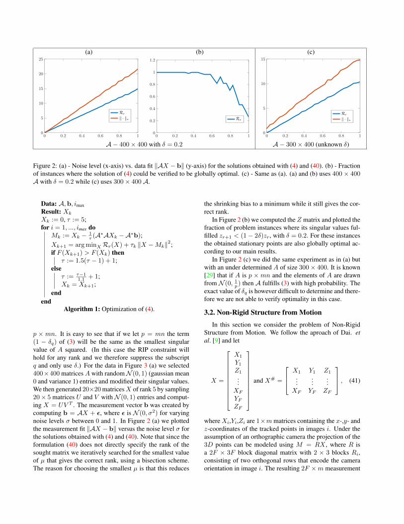
simple real and synthetic applications (some that fulfill (3)and some that do not). For our implementation we use theGIST approach from [16] because of its simplicity. Given acurrent iterate Xk this method solves

Xk+1 = argminX

Rr(X) + τk ‖X −Mk‖2 , (39)

whereMk = Xk− 1τk(A∗AXk−A∗b). Note that if τk = 1

then any fixed point of (39) is a stationary point by Lemma1.1. To solve (39) we use the proximal operator computedin [21].

Our algorithm consists of repeatedly solving (39) for asequence of {τk}. We start from a larger value (τ0 = 5 inour implementation) and reduce towards 1 as long as thisresults in decreasing objective values. Specifically we setτk+1 = τk−1

1.1 + 1 if the previous step was successful inreducing the objective value. Otherwise we increase τ ac-cording to τk+1 = 1.5(τk−1)+1. We outline the approachin Algorithm 1.

3.1. Synthetic Data

We first evaluate the quality of the relaxation on a num-ber of synthetic experiments. We compare the two formula-tions (4) and

minX

µ‖X‖∗ + ‖AX − b‖2. (40)

In Figure 2 (a) we tested these two relaxations on a num-ber of synthetic problems with varying noise levels. Thedata was created so that the operator A fulfills (3) withδ = 0.2. By column stacking an m × n matrix X the lin-ear mapping A can be represented with a matrix A of size

(a) (b) (c)

0 0.2 0.4 0.6 0.8 10

5

10

15

20

25

Rr‖ · ‖∗

0 0.2 0.4 0.6 0.8 10

0.2

0.4

0.6

0.8

1

1.2

Rr

0 0.2 0.4 0.6 0.8 10

5

10

15

Rr‖ · ‖∗

A− 400× 400 with δ = 0.2 A− 300× 400 (unknown δ)

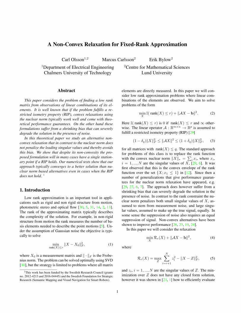
Figure 2: (a) - Noise level (x-axis) vs. data fit ‖AX − b‖ (y-axis) for the solutions obtained with (4) and (40). (b) - Fractionof instances where the solution of (4) could be verified to be globally optimal. (c) - Same as (a). (a) and (b) uses 400× 400A with δ = 0.2 while (c) uses 300× 400 A.

Data: A,b, imaxResult: Xk

Xk := 0, τ := 5;for i = 1, ..., imax do

Mk := Xk − 1τ (A

∗AXk −A∗b);Xk+1 = argminX Rr(X) + τk ‖X −Mk‖2;if F (Xk+1) > F (Xk) then

τ := 1.5(τ − 1) + 1;else

τ := τ−11.1 + 1;

Xk = Xk+1;end

endAlgorithm 1: Optimization of (4).

p × mn. It is easy to see that if we let p = mn the term(1 − δq) of (3) will be the same as the smallest singularvalue of A squared. (In this case the RIP constraint willhold for any rank and we therefore suppress the subscriptq and only use δ.) For the data in Figure 3 (a) we selected400×400 matrices A with randomN (0, 1) (gaussian mean0 and variance 1) entries and modified their singular values.We then generated 20×20 matricesX of rank 5 by sampling20× 5 matrices U and V withN (0, 1) entries and comput-ing X = UV T . The measurement vector b was created bycomputing b = AX + ε, where ε is N (0, σ2) for varyingnoise levels σ between 0 and 1. In Figure 2 (a) we plottedthe measurement fit ‖AX − b‖ versus the noise level σ forthe solutions obtained with (4) and (40). Note that since theformulation (40) does not directly specify the rank of thesought matrix we iteratively searched for the smallest valueof µ that gives the correct rank, using a bisection scheme.The reason for choosing the smallest µ is that this reduces

the shrinking bias to a minimum while it still gives the cor-rect rank.

In Figure 2 (b) we computed the Z matrix and plotted thefraction of problem instances where its singular values ful-filled zr+1 < (1− 2δ)zr, with δ = 0.2. For these instancesthe obtained stationary points are also globally optimal ac-cording to our main results.

In Figure 2 (c) we did the same experiment as in (a) butwith an under determined A of size 300× 400. It is known[29] that if A is p × mn and the elements of A are drawnfrom N (0, 1p ) then A fulfills (3) with high probability. Theexact value of δq is however difficult to determine and there-fore we are not able to verify optimality in this case.

3.2. Non-Rigid Structure from Motion

In this section we consider the problem of Non-RigidStructure from Motion. We follow the aproach of Dai. etal. [9] and let

X =

X1

Y1Z1

...XF

YFZF

and X# =

X1 Y1 Z1

......

...XF YF ZF

, (41)

whereXi,Yi,Zi are 1×mmatrices containing the x-,y- andz-coordinates of the tracked points in images i. Under theassumption of an orthographic camera the projection of the3D points can be modeled using M = RX , where R isa 2F × 3F block diagonal matrix with 2 × 3 blocks Ri,consisting of two orthogonal rows that encode the cameraorientation in image i. The resulting 2F ×m measurement

Drink Pick-up Stretch Yoga

Figure 3: Four images from each of the MOCAP data sets.

Figure 4: Results obtained with (44) (blue dots) and (45) (orage curve) for the four sequences. Data fit ‖RX−M‖F (y-axis)versus rank(X#) (x-axis).

Figure 5: Results obtained with (44) (blue dots) and (45) (orage curve) for the four sequences. Distance to ground truth‖X −Xgt‖F (y-axis) versus rank(X#) (x-axis).

Figure 6: Results obtained with (46) (blue dots) and (47) (orage curve) for the four sequences. Data fit ‖RX−M‖F (y-axis)versus rank(X#) (x-axis).

Figure 7: Results obtained with (46) (blue dots) and (47) (orage curve) for the four sequences. Distance to ground truth‖X −Xgt‖F (y-axis) versus rank(X#) (x-axis) is plotted for various regularization strengths.

matrix M consists of the x- and y-image coordinates or thetracked points. Under the assumption of a linear shape basismodel [5] with r deformation modes, the matrix X# can befactorized intoX# = CB, where the r×3mmatrixB con-tain the basis elements. It is clear that such a factorizationis possible when X# is of rank r. We therefore search forthe matrix X# of rank r that minimizes the residual error‖PX −M‖2F .

The linear operator defined by A(X#) = RX does byitself not obey (3) since there are typically low rank matricesin its nullspace. This can be seen by noting that if Ni is the3 × 1 vector perpendicular to the two rows of Ri, that isRiNi = 0 then Xi

YiZi

= NiCi, (42)

where Ci is any 1 × m matrix, is in the null space of Ri.Therefore any matrix of the form

N(C) =

n11C1 n21C1 n31C1

n12C2 n22C2 n32C2

......

...n1FCF n2FCF n3FCF

, (43)

where nij are the elements ofNi, vanishes underA. Settingeverything but the first row ofN(C) to zero shows that thereis a matrix of rank 1 in the null space of A. Moreover, ifthe rows of the optimal X# spans such a matrix it will notbe unique since we may add N(C) without affecting theprojections or the rank.

In Figure 4 we compare the two relaxations

Rr(X#) + ‖RX −M‖2F (44)

andµ‖X#‖∗ + ‖RX −M‖2F (45)

on the four MOCAP sequences displayed in Figure 3, ob-tained from [9]. These consist of real motion capture dataand therefore the ground truth solution is only approxima-tively of low rank.

In Figure 4 we plot the rank of the obtained solution ver-sus the datafit ‖RX −M‖F . Since (45) does not allow usto directly specify the rank of the sought matrix, we solvedthe problem for 50 values of µ between 1 and 100 (orangecurve) and computed the resulting rank and datafit. Notethat even if a change of µ is not large enough to change therank of the solution it does affect the non-zero singular val-ues. To achieve the best result for a specific rank with (45)we should select the smallest µ that gives the correct rank.Even though (3) does not hold, the relaxation (44) consis-tently gives better data fit with lower rank than (45). Fig-ure 5 also shows the rank versus the distance to the groundtruth solution. For high rank the distance is typically larger

for (44) than (45). A feasible explanation is that when therank is high it is more likely that the row space of X# con-tains a matrix of the type N(C). Loosely speaking, whenwe allow too complex deformations it becomes more diffi-cult to uniquely recover the shape. The nuclear norm’s builtin bias to small solutions helps to regularize the problemwhen the rank constraint is not discriminative enough.

One way to handle the null space of A is to add addi-tional regularizes that penalize low rank matrices of the typeN(C). Dai et al. [9] suggested to use the derivative prior‖DX#‖2F , where the matrix D : RF → RF−1 is a firstorder difference operator. The nullspace of D consists ofmatrices that are constant in each column. Since this im-plies that the scene is rigid it is clear that N(C) is not in thenullspace of D. We add this term and compare

Rr(X#) + ‖RX −M‖2F + ‖DX#‖2F (46)

andµ‖X#‖∗ + ‖RX −M‖2F + ‖DX#‖2F . (47)

Figures 6 and 7 show the results. In this case both the datafit and the distance to the ground truth is consistently bet-ter with (46) than (47). When the rank increases most ofthe regularization comes from the derivative prior leadingto both methods providing similar results.

4. ConclusionsIn this paper we studied the local minima of a non-

convex rank regularization approach. Our main theoreti-cal result shows that if a RIP property holds then there isoften a unique stationary point. Since the proposed relax-ation (4) and the original objective (2) is shown to have thesame global minimizers if ‖A‖ ≤ 1 in [8] this result is alsorelevant for the original discontinuous problem. Our ex-perimental evaluation shows that the proposed approach of-ten gives better solutions than standard convex alternatives,even when the RIP constraint does not hold.

References[1] F. Andersson, M. Carlsson, and C. Olsson. Convex envelopes

for fixed rank approximation. Optimization Letters, pages 1–13, 2017. 1, 2

[2] R. Basri, D. Jacobs, and I. Kemelmacher. Photometric stereowith general, unknown lighting. Int. J. Comput. Vision,72(3):239–257, May 2007. 1

[3] D. Bertsekas. Nonlinear Programming. Athena Scientific,1999. 3

[4] S. Bhojanapalli, B. Neyshabur, and N. Srebro. Global opti-mality of local search for low rank matrix recovery. In An-nual Conference in Neural Information Processing Systems(NIPS). 2016. 3

[5] C. Bregler, A. Hertzmann, and H. Biermann. Recoveringnon-rigid 3d shape from image streams. In IEEE Conferenceon Computer Vision and Pattern Recognition, 2000. 1, 8

[6] E. J. Candes, X. Li, Y. Ma, and J. Wright. Robust principalcomponent analysis? J. ACM, 58(3):11:1–11:37, 2011. 1

[7] E. J. Candes and B. Recht. Exact matrix completion via con-vex optimization. Foundations of Computational Mathemat-ics, 9(6):717–772, 2009. 1

[8] M. Carlsson. On convexification/optimization of func-tionals including an l2-misfit term. arXiv preprintarXiv:1609.09378, 2016. 3, 8

[9] Y. Dai, H. Li, and M. He. A simple prior-free method fornon-rigid structure-from-motion factorization. InternationalJournal of Computer Vision, 107(2):101–122, 2014. 6, 8

[10] C. Eckart and G. Young. The approximation of one matrix byanother of lower rank. Psychometrika, 1(3):211–218, 1936.1

[11] A. Eriksson, T. Thanh Pham, T.-J. Chin, and I. Reid. The k-support norm and convex envelopes of cardinality and rank.In The IEEE Conference on Computer Vision and PatternRecognition, 2015. 2

[12] M. Fazel, H. Hindi, and S. P. Boyd. A rank minimizationheuristic with application to minimum order system approx-imation. In American Control Conference, 2001. 1

[13] R. Garg, A. Roussos, and L. Agapito. A variational approachto video registration with subspace constraints. Int. J. Com-put. Vision, 104(3):286–314, 2013. 1

[14] R. Garg, A. Roussos, and L. de Agapito. Dense variationalreconstruction of non-rigid surfaces from monocular video.In IEEE Conference on Computer Vision and Pattern Recog-nition, 2013. 1

[15] R. Ge, C. Jin, and Y. Zheng. No spurious local minima innonconvex low rank problems: A unified geometric analysis.arXiv preprint, arxiv:1704.00708, 2017. 3

[16] P. Gong, C. Zhang, Z. Lu, J. Huang, and J. Ye. A general it-erative shrinkage and thresholding algorithm for non-convexregularized optimization problems. In International Confer-ence on Machine Learning (ICML), pages 37–45, 2013. 5

[17] C. Grussler and A. Rantzer. On optimal low-rank approxi-mation of non-negative matrices. In 2015 54th IEEE Con-ference on Decision and Control (CDC), pages 5278–5283,Dec 2015. 2

[18] C. Grussler, A. Rantzer, and P. Giselsson. Low-rank opti-mization with convex constraints. CoRR, abs/1606.01793,2016. 2

[19] Y. Hu, D. Zhang, J. Ye, X. Li, and X. He. Fast and accuratematrix completion via truncated nuclear norm regularization.IEEE Transactions on Pattern Analysis and Machine Intelli-gence, 35(9):2117–2130, 2013. 1

[20] V. Larsson and C. Olsson. Convex envelopes for low rankapproximation. In International Conference on Energy Min-imization Methods in Computer Vision and Pattern Recogni-tion, 2015. 2

[21] V. Larsson and C. Olsson. Convex low rank approximation.International Journal of Computer Vision, 120(2):194–214,2016. 1, 2, 3, 5

[22] A. M. McDonald, M. Pontil, and D. Stamos. Spectral k-support norm regularization. In Advances in Neural Infor-mation Processing Systems. 2014. 2

[23] K. Mohan and M. Fazel. Iterative reweighted least squaresfor matrix rank minimization. In Annual Allerton Conferenceon Communication, Control, and Computing, pages 653–661, 2010. 1

[24] T. H. Oh, Y. W. Tai, J. C. Bazin, H. Kim, and I. S. Kweon.Partial sum minimization of singular values in robust pca:Algorithm and applications. IEEE Transactions on PatternAnalysis and Machine Intelligence, 38(4):744–758, 2016. 1

[25] C. Olsson, M. Carlsson, F. Andersson, and V. Larsson. Non-convex rank/sparsity regularization and local minima. Pro-ceedings of the International Conference on Computer Vi-sion, 2017. 2, 3, 4, 5

[26] S. Oymak, A. Jalali, M. Fazel, Y. C. Eldar, and B. Hassibi.Simultaneously structured models with application to sparseand low-rank matrices. IEEE Transactions on InformationTheory, 61(5):2886–2908, 2015. 1

[27] S. Oymak, K. Mohan, M. Fazel, and B. Hassibi. A simplifiedapproach to recovery conditions for low rank matrices. InIEEE International Symposium on Information Theory Pro-ceedings (ISIT), pages 2318–2322, 2011. 1

[28] D. Park, A. Kyrillidis, C. Caramanis, and S. Sanghavi. Non-square matrix sensing without spurious local minima via theburer-monteiro approach. In Proceedings of the 20th Inter-national Conference on Artificial Intelligence and Statistics,AISTATS, pages 65–74, 2017. 3

[29] B. Recht, M. Fazel, and P. A. Parrilo. Guaranteed minimum-rank solutions of linear matrix equations via nuclear normminimization. SIAM Rev., 52(3):471–501, Aug. 2010. 1, 6

[30] C. Tomasi and T. Kanade. Shape and motion from imagestreams under orthography: A factorization method. Int. J.Comput. Vision, 9(2):137–154, 1992. 1

[31] J. Yan and M. Pollefeys. A factorization-based approach forarticulated nonrigid shape, motion and kinematic chain re-covery from video. IEEE Trans. Pattern Anal. Mach. Intell.,30(5):865–877, 2008. 1