Page 1
Degree project
A Non-functional evaluation
of NoSQL Database
Management Systems
Author: Johan Landbris
Supervisor: Mauro Caporuscio
Examiner: Johan Hagelbäck
Date:2015-10-20
Course Code: 2DV00E, 15 credits
Subject: Computer Science
Level: Bachelor
Department of Computer Science
Page 2
Abstract
NoSQL is basically a family name for all Database Management Systems
(DBMS) that is not Relational DBMS. The fast growth of all social networks
has led to a huge amount of unstructured data that NoSQL DBMS is
supposed to handle better than Relational DBMS. Most comparisons
performed are between Relational DBMS and NoSQL DBMS. In this paper,
the comparison is about non-functional properties for different types of
NoSQL DBMS instead. Three of the most common NoSQL types are
Document Stores, Key-Value Stores and Column Stores. The most used
DBMS of those types are MongoDB, Redis and Apache Cassandra. After
working with the databases and performing YCSB Benchmarking the
conclusion is that if the database should handle an enormous amount of data,
Cassandra is most probably best choice. If speed is the most important
property and if all data fits within the memory; Redis is probably the most
well suited database. If the database needs to be flexible and versatile,
MongoDB is probably the best choice.
Page 3
Contents
List of figures 4
1 Introduction 5 1.1 Introduction/Background 5
1.2 Previous research 5 1.3 Purpose and research question/hypothesis 6 1.4 Scope/limitation 6
2 Background/Theory 7
2.1 Relational Database Management Systems 7 2.1.1 ACID Acronym – Relational DBMS properties 7
2.2 NoSQL 8 2.2.1 History about NoSQL 8
2.2.2 BASE Acronym – NoSQL properties 9
2.2.3 CAP Theorem 9 2.2.5 Key-value store 10
2.2.6 Column store 12 2.2.7 Document store 14
3 Method 17
3.1 Scientific approach 17 3.2 Human centered approach 17
3.2.1 Survey 17
3.2.2 Interviews 18
3.3 Yahoo! Cloud Serving Benchmark (YCSB) 19
4 Results/Analysis 20 4.1 Survey 20 4.3 YCSB benchmarking 21
4.2.1 Workload 21 4.2.2 CPU Load 25
4.2.3 Memory Load 26
5 Discussion 27 5.1 Problem solving/results 27 5.2 Method reflection 28
6 Conclusion 29 6.1 Conclusions 29 6.2 Further Research 29
References 30
Page 4
List of figures
Figure 2.1: Typical row in a RDBMS. 7
Figure 2.2: Basic example of a Key-value relation. 10
Figure 2.3: Typical row in a row store. 12
Figure 2.4: Typical row in a column store. 12
Figure 2.5: Relationships with references between documents [15]. 15
Figure 2.6: Embedded document relationship [15]. 15
Figure 3.1: Survey sent to companies. 18
Figure 4.1: Survey and interviews. 20
Figure 4.2: Workload A – 50 % reads, 50 % writes. 21
Figure 4.3: Workload B – 95 % reads, 5 % writes. 22
Figure 4.4: Workload C – 100 % reads. 22
Figure 4.5: Workload D – Read latest workload. 23
Figure 4.6: Workload F – Read-modify-write. 23
Figure 4.7: CPU Load – Average CPU Load. 25
Figure 4.8: Memory load – Average memory load. 26
Page 5
1 Introduction
This chapter gives a brief summary of NoSQL databases along with existing
research regarding the subject. It will also mention the limitations and the
research questions for this thesis project.
1.1 Introduction/Background
NoSQL (usually interpreted as Not only SQL) Data Base Management
Systems (DBMS) are a relatively new kind of databases. NoSQL DBMS are
increasingly used, but Relational DBMS (RDBMS) are still dominating the
market. Over 90% of all systems are using RDBMS [1].
NoSQL is basically a family name for all DBMS that is not
RDBMS. The main reason for the need to invent NoSQL DBMS is the fast
growth of all social networks, which has led to a huge amount of unstructured
data that NoSQL is supposed to handle better than RDBMS. NoSQL DBMS
are supposed to be more scalable and take advantage of new nodes and
clusters without the need of additional management.
NoSQL can infer a lot of different types of databases. Three of
the most common NoSQL types are Document Stores, Key-Value Stores and
Column Stores [2]. The most used DBMS of the types are MongoDB, Redis
and Apache Cassandra. Those are the databases that will be looked at in this
article.
1.2 Previous research
Most benchmarks and comparisons of different DBMS are performed
between different kinds of Relational DBMS [3]. In some cases benchmarks
are performed between Relational databases and NoSQL DBMS, but not by
the most used NoSQL DBMS types [4]. The benchmarks that have been
performed between different NoSQL DBMS are mainly focused on
functional requirements [5]. This article focuses benchmarking on non-
functional properties of the most popular NoSQL DBMS of the most used
NoSQL types, along with a few functional requirement benchmarks. The
properties chosen to be benchmarked are based on what is most of interest to
computer related companies.
Page 6
1.3 Purpose and research question/hypothesis
RQ1. Which is the set of non-functional properties of interest for
industry?
RQ2. Based on RQ1 properties; which is the most versatile NoSQL
DBMS?
Since NoSQL DBMS are becoming more popular, it would be interesting to
understand the set of non-functional properties to take into account when
selecting among the NoSQL DBMS products available on the market.
1.4 Scope/limitation
The non-functional properties that will be investigated in the article are the
following:
Efficiency – Find out which database are the most effective in terms
of CPU- and memory usage.
Performance – Perform benchmarks measuring the time of inserting,
finding and deleting data.
Usability – Discover which one of them that is most user-friendly and
easiest to set up.
Flexibility – Find out which one that is easiest to upgrade and extend.
Availability – Manageability, recoverability, reliability, serviceability
[6].
The research will be limited to three different NoSQL DBMS. The most
popular NoSQL DBMS types are Document stores, Key-value stores and
Column stores [2]. The most used Document store is MongoDB, Redis is the
most used Key-value store and the most popular Column store is Cassandra.
Those three NoSQL DBMS will be used in this thesis project.
Page 7
2 Background/Theory
This chapter contains information about all major technologies and terms that
have been involved in this thesis project. Firstly, a brief summary of
RDBMS, followed by a summary of NoSQL DBMS. The NoSQL summary
goes more into details about different NoSQL types and especially about the
databases that are used in the benchmarks described in the Result chapter.
The ACID, BASE and CAP theorems are also described in this chapter.
2.1 Relational Database Management Systems
This is by far the most popular kind of database management systems.
According to the dbengines website, the three most used DBMS are RDBMS
[2]. They are the “old” kind of databases where tables consist of rows and
columns and each column has a specified type. Information is stored once for
each column. A row only contains values for record, no type information. All
rows in a table have the same columns and are homogenous. A RDBMS must
read the entire row in order to access the requested column data, which many
times lead to an unnecessary amount of reads. That in mind - RDBMS
generally still performs faster reads than writes. Figure 2.1 shows a typical
row in a RDBMS.
Username (String)
First_name (String)
Last_name (String)
Gender (String)
Age (Integer)
JohanL Johan Landbris Male 25
Figure 2.1: Displaying a typical row in a RDBMS.
2.1.1 ACID Acronym – Relational DBMS properties
RDBMS generally follow the ACID acronym. In theory, each letter is
essential. For a very long time, all webpages were able to handle the traffic
with RDBMS and the ACID acronym. However, they lack in availability and
performance when handling huge amount of data [7].
Atomic: Everything in a transaction succeeds or everything fails. All
or nothing rule.
Consistent: A transaction cannot leave the database in an inconsistent
state. Everything is always in order in the database and it never
Page 8
violates any rules – the database is consistent both in the beginning
and in the end of a transaction. Only valid data will be written to the
database. If a transaction violates the consistency rules, the
transaction will not go through and the database will be restored to a
previous state without any failures – a consistent state.
Isolated: Transactions cannot interfere with each other. Every
transaction is completely independent.
Durable: A completed transaction persists even when servers restart,
system failures or power loss etc.
2.2 NoSQL
NoSQL (usually interpreted as Not only SQL) Data Base Management
Systems are a relatively new kind of databases. One definition of NoSQL is
“Different NoSQL databases take different approaches. What they have in
common is that they're not relational. Their primary advantage is that, unlike
relational databases, they handle unstructured data such as word-processing
files, e-mail, multimedia, and social media efficiently” [8]. However, since
NoSQL DBMS comes in so many different shapes, it is hard to give a general
definition. NoSQL is basically a family name for all DBMS that is not
RDBMS. The main reason for the need to invent NoSQL DBMS is the fast
growth of all social networks, which has led to a huge amount of unstructured
data that NoSQL is supposed to handle better than RDBMS. NoSQL DBMS
are supposed to be more scalable and take advantage of new nodes and
clusters without the need of additional management. NoSQL should therefore
be cheaper to maintain than RDBMS, both because of less management and
the horizontal scalability with many cheaper servers instead of a few
expensive servers.
2.2.1 History about NoSQL
The term NoSQL was first used in 1998 by Carlo Strozzi [9]. He had an open
source project which did not offer an ordinary SQL interface. He called his
database “NoSQL” and stored all data as ASCII files which was a first step
towards something else than RDBMS. This, however, does not have anything
to do with today’s NoSQL RDBMS. The term has no scientific accepted
definition since it is such a broad term.
Page 9
2.2.2 BASE Acronym – NoSQL properties
The BASE acronym is usually used to describe properties of NoSQL
databases. It has some similarities to the ACID acronym which instead is
used to describe Relational DBMS properties. See the ACID Acronym –
Relational DBMS properties chapter (2.1.1) for differences between the two
acronyms.
Basic Availability: The system does guarantee the availability of the
data - every request will be answered. Even if the database has
multiple failures, it should be available. NoSQL DBMS usually
spreads data to multiple storage systems and therefor the fault
tolerance is spread. Even if one event fails the fault handling is
performed in that specific data store and the whole system does not go
down and is still available.
Soft-state: The system state may change over time, even without any
operation performed, therefore – the system state is always soft.
Eventual consistency: The system will eventually be consistent once
it stops receiving input. Consistency infers that a transaction cannot
leave the database in an inconsistent state. Everything is always in
order in the database and it never violates any rules – the database is
consistent both in the beginning and in the end of a transaction. Only
valid data will be written to the database. If a transaction violates the
consistency rules, the transaction will not go through and the database
will be restored to a previous state without any failures – a consistent
state.
2.2.3 CAP Theorem
The CAP theorem explains the theoretical gap between ACID and BASE
compliant databases and it claims that it is impossible for a database to be all
three letters [10].
Consistency: A transaction cannot leave the database in an
inconsistent state. Everything is always in order in the database and it
never violates any rules – the database is consistent both in the
beginning and in the end of a transaction. Only valid data will be
written to the database. If a transaction violates the consistency rules,
the transaction will not go through and the database will be restored to
a previous state without any failures – a consistent state.
Availability: The given system is available when needed – there will
always be a response to any request.
Page 10
Partition Tolerance: A system should continue to operate even when
there is partial data loss, temporary system failure or interruption. A
single node failure should not cause the system to stop working. No
failure other than total network failure is allowed to cause the system
to behave differently.
2.2.4 Clustering
A big difference between NoSQL DBMS and RDBMS is that NoSQL
generally cluster much easier, which is a very common requirement in most
large systems these days. In context of databases, clustering infers that many
instances or servers connect to the same database. A major advantage with
clustering is the fault tolerance, since there are several servers or instances
running. If one server or instance is shut down, a user can connect to one of
the servers or instances still running. Another advantage is that a cluster in
general connects a user to the server or instance with the least load at the
connecting moment.
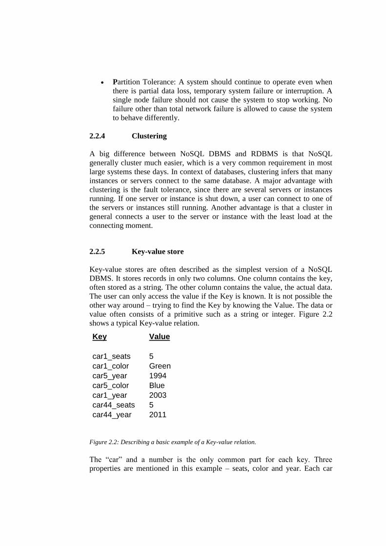
2.2.5 Key-value store
Key-value stores are often described as the simplest version of a NoSQL
DBMS. It stores records in only two columns. One column contains the key,
often stored as a string. The other column contains the value, the actual data.
The user can only access the value if the Key is known. It is not possible the
other way around – trying to find the Key by knowing the Value. The data or
value often consists of a primitive such as a string or integer. Figure 2.2
shows a typical Key-value relation.
Key Value
car1_seats 5
car1_color Green
car5_year 1994
car5_color Blue
car1_year 2003
car44_seats 5
car44_year 2011
Figure 2.2: Describing a basic example of a Key-value relation.
The “car” and a number is the only common part for each key. Three
properties are mentioned in this example – seats, color and year. Each car
Page 11
does not have to store every property and no primary key. There are many
different key-value stores on the market and they work a bit differently. This
is however a basic explanation that applies to most of them. Redis is an open-
source key-value database created by Salvatore Sanfilippo in 2009 [11]. The
company started with a few sponsors along with donations, but it is now
sponsored by Pivotal. Redis is now by far the most used key-value store [12].
Redis is an in-memory key-value store. A major difference between Redis
and many other key-value stores is that Redis can handle a large number of
different datatypes, which makes it very versatile. The value can for example,
along with primitive datatypes, also consist of lists, hashes or sets. Redis
handles the whole dataset in memory until data is written to disc
asynchronously. The administrator can decide how often Redis should save
the data from memory to disc. If the system crashes, some of the data still in
memory might get lost if it is not saved to disc. Redis is therefore considered
to be a CP in the CAP theorem. Please see the BASE chapter (2.2.2),
especially the BA part for more information about availability along with the
CAP chapter (2.2.3). Redis supports the following languages:
C
C#
C++
Clojure
Dart
Erlang
Go
Haskell
Java
JavaScript
Lisp
Lua
Objective-C
Perl
PHP
Python
Ruby
Scala
Smalltalk
Tcl
Redis supports the following operating systems:
BSD
Linux
OS X
Windows
Page 12
2.2.6 Column store
A column store has all data organized and stored in columns instead of the
usual RDBMS rows. A row in a column store has some kind of row id, where
each column value is associated with each other. Instead of searching each
row, column stores only focus on the column that is of interest. That is, in
theory, faster than a row store. An example: A database has 10.000 users,
which equals 10.000 rows, one for each user. If the user wants Username and
Gender for a user, a row store must search each column for each row, which
can be up to 10.000x5=50.000 column values. Figure 2.3 shows a typical row
in a row store.
Username First_name Last_name Gender Age
JohanL Johan Landbris Male 25
Figure 2.3: Displaying a typical row in a row store.
If the same search is performed in a column oriented store, the maximum
column values that can be looked into are 10.000x2=20.000 since column
stores only focus on the columns that are relevant. Figure 2.4 highlights the
difference between a row store and a column store.
Username First_name Last_name Gender Age
JohanL Johan Landbris Male 25
Figure 2.4: Highlighting the relevant columns in a column store.
Apache Cassandra is a combination of Google Bigtable and Amazon
Dynamo that was incubated in Facebook. In July 2008 Cassandra became an
open-source and in March 2009 Cassandra became an Apache project [13].
Cassandra is a peer-to-peer distributed system with nodes, where data is
distributed to all nodes within the cluster. All nodes are the same and equal in
Cassandra, meaning there is no central master node. Data is partitioned
among all nodes in a cluster. Each node communicates with each other and
exchanges information across the cluster every second, which is referred to as
a gossip protocol. A collection of all related nodes are called Data center. A
column family is a container with a collection of rows. Every row contains
columns which are in order. Column families represent the structure of the
data. New nodes can be added to the Cassandra cluster without the need to
shut down the system. Cassandra satisfies Availability and Partition tolerance
(AP) according to the CAP theorem, since data is not written to disc until the
Mem-Table is full. See the CAP chapter (2.2.3) for a more detailed
explanation. Cassandra writes data to disc in the following sequence:
Page 13
1. Commit log: Data is first written to a commit log, where all data is
saved as a backup if the system should crash.
2. Node: Data is sent to an appropriate Node. When the node gets the
data it saves it in a local log and sends it to the correct mem-table for
the column family.
3. Mem-table: In-memory temporarily storage for Cassandra, works a lot
like key-value pairs. When the memory is full or when time is up
(decided by the user), the mem-table is flushed to disc, SSTable.
4. SSTable (Stored String Table): SSTable is the disc store for
Cassandra. Cassandra makes sure data ends up in the correct SSTable
with help of a Bloom filter.
5. Bloom filter: Bloom filters basically test whether the incoming data is
a member of this set or SSTable. Bloom filter is also used for read
requests. The filter checks the probability for a SSTable to contain the
requested data.
6. When all column families from the Commit log are pushed to disc,
they are deleted.
7. Compaction: Cassandra can free disc space by merging large
accumulated data files. Data is indexed, sorted, merged and collected
from many old SSTables into a new SSTable. This makes scan time a
lot faster.
Cassandra reads data from disc in the following sequence:
1. Cassandra checks the Bloom filter, which decides the probability for
the SSTable to contain the requested data.
2. If the probability/chance is good, Cassandra looks at the partition key
cache which is a cache of the partition index which is a list of primary
keys and start position of data, for tables.
If an index entry is found in cache: The compression map is used to find the
block containing the data. The requested data is merged from all SSTables, or
if the data is found in the mem-table, for faster future reads and is returned.
If an index entry is not found in cache: Cassandra searches the
partition summary, a subset of the partition index, to determine the
approximate disc location of the index entry. Depending on the results from
the partition summary, Cassandra performs a sequential read of columns in
the SSTables of interest. Correct data is merged and returned. Cassandra
supports the following languages:
Page 14
C
C#
C++
Clojure
Erlang
Go
Haskell
Java
JavaScript
Perl
PHP
Python
Ruby
Scala
Cassandra supports the following operating systems:
BSD
Linux
OS X
Windows
2.2.7 Document store
Document stores or document-oriented databases are one of the most
common NoSQL types along with Column store, Key-value store and Graph
store. They are in some ways a sub category of Key-value stores since each
document is recognized with a key. Document stores contain, as the name
reveals, documents. All data is stored in the document itself and is totally
schema-free without tables, row or columns. Each document is totally
independent from the others. This makes document-oriented databases
flexible. They can simply add or delete a field from a document without
disturbing other documents. In contrast to relational database management
systems there is no need to have any empty fields. Common document
encodings are for example JSON, BSON and XML.
MongoDB was developed in 2007 by 10gen and was available
as open source in 2009 with the possibility for a commercial license [14].
MongoDB has a flexible schema, in contrast to most relational databases
where the developer must decide the schema for each table before any data is
inserted. Instead of tables, MongoDB uses collections. A collection is a group
of documents, but documents within the collection can still have different
fields. Documents in a collection usually fill the same purpose though.
MongoDB documents are stored in BSON format, which is a binary version
of JSON documents. BSON can contain more data types than JSON.
Documents can be linked or referenced to each other with a key. Embedded
Page 15
documents are an alternative to references, where all information is
embedded in a single document instead of using references to many
documents. Generally, embedded documents provide better performance but
reference documents are more flexible. Figure 2.5 shows relationships with
references between documents and Figure 2.6 shows embedded documents
relationships.
Figure 2.5: Displaying relationships with references between documents [15].
Figure 2.6: Displaying embedded document relationship [15].
Page 16
MongoDB supports the following languages:
Actionscript
C
C#
C++
Clojure
ColdFusion
D
Dart
Delphi
Erlang
Go
Groovy
Haskell
Java
JavaScript
Lisp
Lua
MatLab
Perl
PHP
PowerShell
Prolog
Python
R
Ruby
Scala
Smalltalk
MongoDB supports the following operating systems:
Linux
OS X
Solaris
Windows
Page 17
3 Method This chapter describes the approach throughout the whole thesis project, along with
some specific technical solutions.
3.1 Scientific approach
To discover which non-functional properties for databases that was most
important for companies, a survey was sent out to computer related
companies.. Phone interviews were conducted with people working at
different computer related companies. YSCB (Yahoo! Cloud Serving
Benchmark) was used to benchmark the non-functional properties based on
the survey and interview answers.
3.2 Human centered approach
The information about which non-function properties that should be
benchmarked and used as the base for this research was decided from a
survey along with interviews with computer related companies.
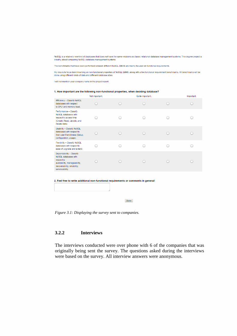
3.2.1 Survey
The survey was sent as a link to 20 companies. It was created and handled
online with the help of a webpage, SurveyMonkey[16]. All survey answers
were anonymous. Figure 3.1 shows the survey sent out to companies.
Page 18
Figure 3.1: Displaying the survey sent to companies.
3.2.2 Interviews
The interviews conducted were over phone with 6 of the companies that was
originally being sent the survey. The questions asked during the interviews
were based on the survey. All interview answers were anonymous.
Page 19
3.3 Yahoo! Cloud Serving Benchmark (YCSB)
Since NoSQL DBMS still are quite new, there are not that many good and
fair benchmarking tools. There are, however, a lot of existing benchmarking
tools for RDBMS but they are, for obvious reasons, not compatible with
NoSQL DBMS. Most of the existing NoSQL tools are either provided by the
database company itself, or not compatible with different NoSQL types. It is
hard to develop a benchmarking tool for all NoSQL types (See the Column
Store (2.2.5), Key-value Store (2.2.4) and Document Store (2.2.6) chapters
for additional information about the differences in NoSQL DBMS). The
Yahoo! Cloud Serving Benchmark was chosen for this project, since it is the
most fair, independent and versatile choice.
Yahoo! Cloud Serving Benchmark is not very useful by itself,
but it provides a good framework for benchmarking NoSQL DBMS [17]. The
YCSB client is a generator of workloads. YCSB provides a few typical
workloads for the most common operations for a DBMS. Basically, the
YCSB client generates a workload. The workload could be one of the core
workloads pre-defined by YCSB or the user can create a customized
workload. The YCSB client is connected to an interface layer of client code
for the DBMS of the user’s choice. A workload is then run through the YCSB
client and is connected to the chosen database server. Here follows a
description of each workload:
Workload A - Update heavy workload: This workload has a mix of
50/50 reads and writes. An application example is a session store
recording recent actions.
Workload B - Read mostly workload: This workload has a 95/5
reads/write mix. Application example: photo tagging; add a tag is an
update, but most operations are to read tags.
Workload C - Read only: This workload is 100% read. Application
example: user profile cache, where profiles are constructed elsewhere
(e.g., Hadoop).
Workload D - Read latest workload: In this workload, new records are
inserted, and the most recently inserted records are the most popular.
Application example: user status updates; people want to read the
latest.
Workload E - Short ranges: In this workload, short ranges of records
are queried, instead of individual records. Application example:
threaded conversations, where each scan is for the posts in a given
thread (assumed to be clustered by thread id).
Workload F - Read-modify-write: In this workload, the client will
read a record, modify it, and write back the changes. Application
Page 20
example: user database, where user records are read and modified by
the user or to record user activity.
4 Results/Analysis
This chapter displays results from the surveys and interviews along with
YCSB benchmark results.
4.1 Survey
Figure 4.1 shows a diagram with survey and interview answers from
computer related companies. The question asked is “How important are the
following non-functional properties when deciding database?”. Rating 1
infers not important and rating 5 infers important.
Figure 4.1: Survey and interviews.
The survey displayed that according to the companies; Dependability
(availability, manageability, recoverability, reliability, serviceability) was the
most important non-functional property, followed by Performance (access
time - Create, Read, Update, and Delete data) and Efficiency (CPU- and
memory load).
Page 21
4.2 Interviews
The interviews were conducted over phone and they gave a more versatile
picture of the non-functional properties of interest. They generated very
different responses depending on the database size and what the database was
used for. Some companies with different databases had different non-
functional property ranking for each database. However, in general the result
was very similar to the Survey answers.
4.3 YCSB benchmarking
Technical specification for the computer used when performing YCSB
benchmarking:
CPU: Intel Core i5 3570k, 3,4 Ghz
Harddrive: Seagate Barracuda ST1000DM003 1TB 7200 RPM
Memory: 8 GB DDR3 1600MHz
Operating system: Ubuntu 14.04.2 LTS
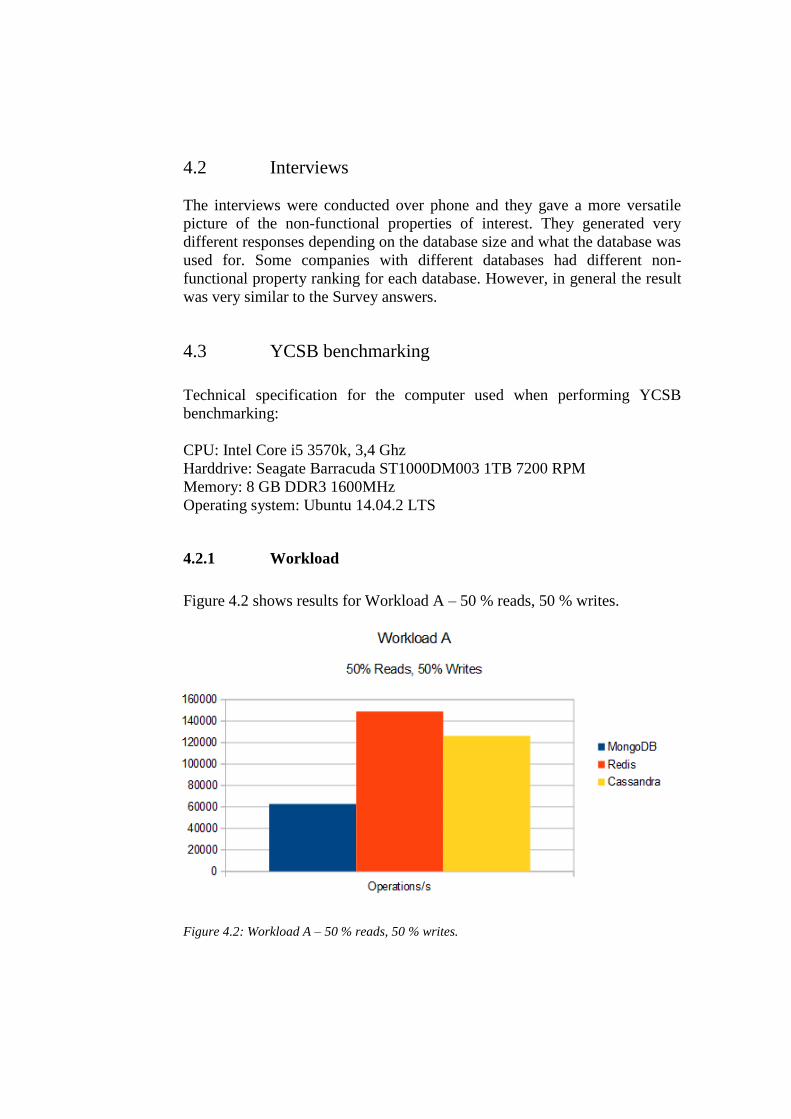
4.2.1 Workload
Figure 4.2 shows results for Workload A – 50 % reads, 50 % writes.
Figure 4.2: Workload A – 50 % reads, 50 % writes.
Page 22
Figure 4.3 shows results for Workload B – 95 % reads, 5 % writes.
Figure 4.3: Workload B – 95 % reads, 5 % writes.
Figure 4.4 shows results for Workload C – 100 % reads.
Figure 4.4: Workload C – 100 % reads.
Page 23
Figure 4.5 shows results for Workload D – Read latest workload.
Figure 4.5: Workload D – Read latest workload.
Figure 4.6 shows results for Workload F – Read-modify-write.
Figure 4.6: Workload F – Read-modify-write.
Page 24
Redis benchmark results for Workload A (50% reads and 50% writes), is
better than Workload B (95 % reads and 5 % writes) and Workload C (100 %
reads). Redis therefore generally writes faster than it reads. The reason for
this is because Redis initially only writes to the memory. Redis handles the
whole dataset in memory until data is written to disc asynchronously. The
administrator decides how often Redis should save the data from memory to
disc. When performing a read on the other hand, Redis sometimes needs to
look for data on disc if it is not found in memory.
In Workload A (50% reads and 50% writes), Cassandra is
performing better than Workload B (95 % reads and 5 % writes) and
Workload C (100 % reads). It means that Cassandra writes data faster than it
reads. This was never the case when dealing with traditional SQL databases
since they are implemented differently that Cassandra. When writing,
Cassandra first writes all data to memory until it is full and flushed to disc.
Reads on the other hand almost always need access the permanent disc
storage, SSTable, along with searching the memory storage, mem-table (See
chapter 2.2.6 Column store for more information about the Cassandra
write/read sequence). In Workload D (Read latest workload) Cassandra
performs very well since in most cases it has to read from the mem-table
since the mem-table most likely has not yet been flushed to disc.
MongoDB benchmark shows that Workload B (95 % reads and
5 % writes) and Workload C (100 % reads) outperforms Workload A (50%
reads and 50% writes). MongoDB therefore reads way faster than it writes
much like a traditional RDBMS. Even benchmark results from Workload D
(Read latest workload) outperforms Workload A (50% reads and 50%
writes).
Redis is the fastest of the three in almost all cases besides
Workload D where Cassandra is a bit faster. MongoDB is the slowest in all
cases besides Workload F where Cassandra is the slowest.
Page 25
4.2.2 CPU Load
Figure 4.7 shows results for average CPU load.
Figure 4.7: CPU Load – Average CPU Load.
Redis’s CPU load was around 55% for each benchmark, way lower than both
Cassandra and MongoDB. The reason is probably because of its in-memory
approach. Cassandra’s average CPU load was around 88% and average CPU
load for MongoDB was about 85% throughout all benchmarks.
Page 26
4.2.3 Memory Load
Figure 4.8 shows results for average memory load.
Figure 4.8: Memory load – Average memory load.
Redis’s memory load was about 25% for each benchmark. It was much
higher than both Cassandra’s and MongoDB’s. Just as the CPU load, the
reason is probably because its in-memory approach. For Cassandra, memory
load was a bit higher when writing than reading with an average of around
14%. MongoDB had an average memory load on about 18% for each
benchmark.
Page 27
5 Discussion
This chapter analyzes and discusses the results displayed in chapter 4 –
Results/Empirical data. It also includes a reflection regarding method choices
throughout the thesis project.
5.1 Problem solving/results
Redis turned out to be the fastest, quite far ahead of the other two in almost
every benchmark. Cassandra was often the second fastest and MongoDB the
slowest. Redis Memory load was the highest and its CPU load was the
lowest. Cassandra and MongoDB were quite equal in both CPU load and
Memory load.
The reason for Redis's outstanding speed is probably because
Redis is less complicated than the other two since it is a Key-value store (See
chapter 2.2.5 for more information about Key-value stores). Redis also
handles all data in memory which makes it rapidly fast. That is why Redis's
average Memory load was above Cassandra's and MongoDB's. I found Redis
to be easy to both set up and work with.
Cassandra performed good in each benchmark. It is not the best
but not the worst either. Cassandra's main advantage over the other two
databases is its scalability and clustering possibilities. A Cassandra cluster
scales linearly and is relatively easy to set up. However, Cassandra is the
most difficult to work with and it is quite hard to make changes to it. It is
very different in both setup and commands compared to traditional relational
DBMS’s.
MongoDB performed the worst in almost every benchmark.
The main advantage of MongoDB is its flexibility. Each document could
have completely different fields even within the same collection, which
makes it very versatile (See chapter 2.2.7.1.1 for more information about
MongoDB Function). I found MongoDB to be the easiest to work with, since
it reminds a lot of Relational DBMS. MongoDB scales well, but not as good
as linearly.
In one sense Redis, Cassandra and MongoDB are very similar
since they after all are databases that handle and stores data. When looking
closer, they are however very different. I could recommend all three
databases, totally depending on the usage. If the database should handle an
enormous amount of data, Cassandra is most probably the way to go.
However, very few applications and systems are in need for such large
amount of data that it should be worth it. If speed is the main thing, Redis is
probably the most well suited choice if the operations are not too advanced
and the database size can fit within the memory. If the database needs to be
Page 28
flexible and not really sure how it should be designed or how big it will be,
MongoDB is probably a good choice.
Since each database is best suited for some specific tasks, one
common option in bigger systems is to combine different database types
within the same system where each database is best suited for its specific
task. When choosing database the CAP theorem (see chapter 2.2.3) can also
be considered, were Redis and MongoDB is considered to be CP and
Cassandra is AP.
In almost every case, MongoDB is a good choice. It is easy to
use and understand and it is relatively fast even though it is slower than
Cassandra and Redis. It is also flexible and scales quite well. Average-sized
systems very seldom need the speed of Redis or the scalability of Cassandra,
so in these cases MongoDB is the most versatile NoSQL DBMS of the three.
But, once again, it completely depends on the situation.
5.2 Method reflection
I should have asked more companies to get a clearer picture of what non-
functional properties that was of interest. Since only 7 companies responded
the survey and 6 interviews were conducted, the answer may not be totally
reliable.
I would also have liked to perform a few benchmarks using
clusters, since that is the case in many big companies. This is however not
very easy considering the limited time and resources for a thesis project.
Overall I am relatively pleased with my choice of method.
Page 29
6 Conclusion
This chapter gives a brief summary of the conclusion of the thesis project. It
also suggests further research regarding similar research area.
6.1 Conclusions
RQ1. Which is the set of non-functional properties of interest for
industry?
RQ2. Based on RQ1 properties; which is the most versatile NoSQL
DBMS?
Research question 1 is not answered since the survey and interviews did not
generate enough answers from computer related companies.
Research question 2 is answered, but since the question is based
on research question 1, the answer is a bit subjective. Cassandra is most
probably the best choice if the database should handle an enormous amount
of data. Redis is probably the most well suited database if speed is the most
important property and if all data fits within the memory. MongoDB is
probably the best choice if the database needs to be flexible and versatile.
6.2 Further Research
I am suggesting performing benchmarks using clusters for each database. To
find out if it is easily done and if it scales well without too much loss in
performance and usability.
Page 30
References
[1] RDBMS dominate the database market, but NoSQL systems are catching
up. URL: http://www.db-engines.com/en/blog_post/23.
URL last accessed 2015-10-11.
[2] DB-engines ranking. URL: http://www.db-engines.com/en/ranking.
URL last accessed 2015-10-11.
[3] M. Åsberg. “Jämförelse av Oracle och MySQL med fokus på användning
i laborationer för universitetsutbildning”. Institutionen för datavetenskap,
2008.
[4] E. Chavez Alcarraz, M. Moraga. “Linked data performance in different
databases: Comparison between SQL and NoSQL databases”. KTH, School
of Technology and Health, 2014.
[5] Comparison of relational database systems. URL:
https://www.digitalocean.com/community/tutorials/sqlite-vs-mysql-vs-
postgresql-a-comparison-of-relational-database-management-systems.
URL last accessed 2015-10-11.
[6] Defining database availability.
URL: https://datatechnologytoday.wordpress.com/2013/06/24/defining-
database-availability/. URL last accessed 2015-10-11.
[7] ACID versus BASE for database transactions. URL:
http://www.johndcook.com/blog/2009/07/06/brewer-cap-theorem-base/.
URL last accessed 2015-10-11.
[8] Leavitt and Neal. Will NoSQL Databases Live Up to Their
Promise?. Leavitt Communications, 2010.
[9] World of NoSQL databases.
URL: http://www.leopard.in.ua/2013/11/08/nosql-world/.
URL last accessed 2015-10-11.
[10] Brewer’s CAP Theorem. URL:
http://www.julianbrowne.com/article/viewer/brewers-cap-theorem.
URL last accessed 2015-10-11.
[11] Redis documentation. URL: http://www.redis.io/documentation.
URL last accessed 2015-10-11.
Page 31
[12] DB-Engines ranking of Key-value stores. URL: http://www.db-
engines.com/en/ranking/key-value+store. URL last accessed 2015-10-11.
[13] Cassandra documentation. URL: http://wiki.apache.org/cassandra/.
URL last accessed 2015-10-11.
[14] MongoDB documentation. URL: http://www.mongodb.org/about/.
URL last accessed 2015-10-11.
[15] MongoDB data model design. URL:
http://docs.mongodb.org/manual/core/data-model-design/.
URL last accessed 2015-10-11.
[16] Survey creating webpage. URL: https://sv.surveymonkey.com/.
URL last accessed 2015-10-11.
[17] Yahoo! Cloud Serving Benchmark.
URL: https://www.github.com/brianfrankcooper/YCSB/wiki.
URL last accessed 2015-10-11.


![Fundamentals of Database Systems - [NoSQL]](https://static.documents.pub/doc/80x56/621c7a5739274824355fa21e/fundamentals-of-database-systems-nosql.jpg)


