A Non-singular Horizontal Position Representation Kenneth Gade (Norwegian Defence Research Establishment (FFI)) (Email : Kenneth.Gade@ffi.no) Position calculations, e.g. adding, subtracting, interpolating, and averaging positions, de- pend on the representation used, both with respect to simplicity of the written code and accuracy of the result. The latitude/longitude representation is widely used, but near the pole singularities, this representation has several complex properties, such as error in latitude leading to error in longitude. Longitude also has a discontinuity at t180x. These properties may lead to large errors in many standard algorithms. Using an ellipsoidal Earth model also makes latitude/longitude calculations complex or approximate. Other common represen- tations of horizontal position include UTM and local Cartesian ‘ flat Earth ’ approximations, but these usually only give approximate answers, and are complex to use over larger dis- tances. The normal vector to the Earth ellipsoid (called n-vector) is a non-singular position representation that turns out to be very convenient for practical position calculations. This paper presents this representation, and compares it with other alternatives, showing that n-vector is simpler to use and gives exact answers for all global positions, and all distances, for both ellipsoidal and spherical Earth models. In addition, two functions based on n-vector are presented, that further simplify most practical position calculations, while ensuring full accuracy. KEY WORDS 1. Position representations. 2. Position calculations. 3. Implementation simplicity. 4. Non-singular representation. 1. INTRODUCTION. Calculations involving global position, i.e. position relative to the Earth, are central in many fields, such as navigation, radar/sonar cal- culations, geodesy, and vehicle guidance and control. In these calculations, the position can be represented by different mathematical quantities, each with its own properties. There are several well-known representations for global position, such as latitude/longitude, UTM (Universal Transverse Mercator (Snyder, 1987)), and Cartesian 3D vector (Earth-Centred-Earth Fixed). These position representations will be discussed in Section 3, focusing on their limitations, and how their proper- ties may induce significant errors in common calculations. Many of the problems and limitations of these alternatives are avoided if using the normal vector to the Earth ellipsoid (called n-vector) to represent the position. Although this represen- tation has been briefly mentioned in some texts (e.g. Aeronautical Systems Div Wright-Patterson AFB OH, 1986) a thorough presentation of this alternative, THE JOURNAL OF NAVIGATION (2010), 63, 395–417. f The Royal Institute of Navigation doi:10.1017/S0373463309990415 Note: A shorter presentation of this topic, including downloadable code, is available at www.navlab.net/nvector
Transcript
A Non-singular Horizontal PositionRepresentation
Kenneth Gade
(Norwegian Defence Research Establishment (FFI))(Email : [email protected])
Position calculations, e.g. adding, subtracting, interpolating, and averaging positions, de-pend on the representation used, both with respect to simplicity of the written code and
accuracy of the result. The latitude/longitude representation is widely used, but near the polesingularities, this representation has several complex properties, such as error in latitudeleading to error in longitude. Longitude also has a discontinuity at t180x. These propertiesmay lead to large errors in many standard algorithms. Using an ellipsoidal Earth model also
makes latitude/longitude calculations complex or approximate. Other common represen-tations of horizontal position include UTM and local Cartesian ‘flat Earth’ approximations,but these usually only give approximate answers, and are complex to use over larger dis-
tances. The normal vector to the Earth ellipsoid (called n-vector) is a non-singular positionrepresentation that turns out to be very convenient for practical position calculations. Thispaper presents this representation, and compares it with other alternatives, showing that
n-vector is simpler to use and gives exact answers for all global positions, and all distances,for both ellipsoidal and spherical Earth models. In addition, two functions based on n-vectorare presented, that further simplify most practical position calculations, while ensuring full
accuracy.
KEY WORDS
1. Position representations. 2. Position calculations. 3. Implementation simplicity.
4. Non-singular representation.
1. INTRODUCTION. Calculations involving global position, i.e. positionrelative to the Earth, are central in many fields, such as navigation, radar/sonar cal-culations, geodesy, and vehicle guidance and control. In these calculations, theposition can be represented by different mathematical quantities, each with its ownproperties. There are several well-known representations for global position, suchas latitude/longitude, UTM (Universal Transverse Mercator (Snyder, 1987)), andCartesian 3D vector (Earth-Centred-Earth Fixed). These position representationswill be discussed in Section 3, focusing on their limitations, and how their proper-ties may induce significant errors in common calculations. Many of the problemsand limitations of these alternatives are avoided if using the normal vector to theEarth ellipsoid (called n-vector) to represent the position. Although this represen-tation has been briefly mentioned in some texts (e.g. Aeronautical Systems DivWright-Patterson AFB OH, 1986) a thorough presentation of this alternative,
THE JOURNAL OF NAVIGATION (2010), 63, 395–417. f The Royal Institute of Navigationdoi:10.1017/S0373463309990415
Note: A shorter presentation of this topic, including downloadable code, is available at www.navlab.net/nvector
including comparisons with the more well known representations is not found inthe literature. This paper will present the n-vector alternative by first discussing thegeometrical properties of n-vector in Section 4. Section 5 presents various n-vectorcalculations, illustrating the fact that calculations involving n-vector are in generalremarkably simple. To simplify implementation further, two functions are presented,which turn out to cover a majority of practical position calculations. In Section 6,several examples comparing the use of latitude/longitude with n-vector for specificcalculations are studied. The practical usefulness of n-vector in real-life applicationsis the topic of Section 7, where the experience is that research groups prefer usingn-vector in many of their position calculations after becoming familiar with it.
2. NOTATION. A unified and stringent notation is of utmost importancewhen describing the kinematics of multiple rotating systems, and a full notationsystem with definitions of the central quantities has been developed by the author(to be published). A short, simplified extract from this system, with only the sym-bols relevant in this paper, is given below.
2.1. Coordinate frame. A coordinate frame is defined as a combination of a point(origin), representing position, and a set of basis vectors, representing orientation.Thus, a coordinate frame has 6 degrees of freedom and can be used to represent theposition and orientation of a rigid body. A listing of the specific coordinate framesrelevant in this paper is found in Appendix A.
2.2. General notation. A general vector can be represented in two different ways(McGill and King, 1995), (Britting, 1971) :
’ ~xx (Lower case letter with arrow): Coordinate free/geometrical vector (notdecomposed in any coordinate frame)
’ xA (Bold lower case letter with right superscript) : Vector decomposed/represented in a specific frame (column matrix with three scalars)
The physical world to be described by the kinematics is modelled in terms of co-ordinate frames. Hence, quantities such as position, angular velocity, etc. relate onecoordinate frame to another. To make a quantity unique, the two frames in questionare given as right subscript, as shown in Table 1. Note that in most examples inTable 1, only the position or the orientation of the frame is relevant, and the contextshould make it clear which of the two properties is relevant (for instance, only theorientation of a frame written as right superscript is relevant, since it denotes theframe of decomposition, where only the direction of the basis vectors matters). Ifboth the position and the orientation of the frame are relevant, the frame is under-lined to emphasize that fact. For generality, the vectors in Table 1 are written incoordinate free form, but before implementation in a computer, they must bedecomposed in a selected frame (e.g. vAB
C is the angular velocity ~vvAB decomposed inframe C).
3. STANDARD POSITION REPRESENTATIONS. Before intro-ducing n-vector, the standard position representations are discussed as a backgroundfor comparison.
396 KENNETH GADE VOL. 63
3.1. Cartesian 3D vector. When representing the position of a general coordinateframe B relative to a reference coordinate frame A, the most intuitive quantity to useis the position vector from A to B, decomposed in A, pAB
A . This paper focuses onglobal positioning, and using the frames defined in Appendix A, we can represent theposition of a body frame (B) relative to the Earth (E), by using pEB
E . This (Cartesian)vector is often referred to as Earth Centred Earth Fixed (ECEF) vector. While thisrepresentation is non-singular and intuitive, there are many situations where otherrepresentations are more practical when positioning an object relative to the Earthreference ellipsoid.
3.2. Separating horizontal and vertical components. For many position calcu-lations, it is desirable and most intuitive to treat horizontal and vertical positions in-dependently. This is for instance useful in a navigation system, where horizontal andvertical position are usually measured by different sensors at different points in time,or in a vehicle autopilot, where horizontal and vertical position are often controlledindependently. In such applications, we usually compare two horizontal positions,and thus we need a quantity for representing horizontal position independently of thevertical height/depth. It should thus be possible to represent horizontal positionwithout considering the vertical position, and vice versa. If the vector pEB
E is used, thehorizontal and vertical positions are not separated as desired.
3.2.1. Latitude and longitude. A common solution for obtaining separate hori-zontal and vertical positions is the use of latitude, longitude and height/depth (relatedto a reference ellipsoid, discussed in Section 4.1). However, this representation has asevere limitation; the two singularities at latitudes t90x, where longitude is un-defined. In addition, when getting close to the singularities, the representation exhibitsconsiderable non-linearities and extreme latitude dependency, leading to reducedaccuracy in many algorithms, as exemplified in Section 6. Thus, these coordinates arenot suitable for algorithms that should be able to calculate positions far north or farsouth. In addition, calculations neart180x longitude become complicated due to thediscontinuity.
3.2.2. Local Cartesian coordinate frame ( flat Earth assumption). Another com-mon solution for separating the horizontal and vertical components is to introduce alocal Earth-fixed Cartesian coordinate frame, with two axes forming a horizontaltangent plane to the reference ellipsoid at a specified tangent point. Assuming severalcalculations are needed in a limited area, position calculations can be performedrelative to this system to get approximate horizontal and vertical components. Thiscoordinate frame is not used as a global position representation (since the local origin
Table 1. Symbols used to describe basic relations between two coordinate frames.
Quantity Symbol Description
Position vector ~ppAB A vector whose length and direction is such that it goes from the origin
of frame A to the origin of frame B, i.e. the position of B relative to A.
Velocity vector ~vvAB The velocity of the origin of frame B, relative to frame A. The underline
indicates that both the position and orientation of A is relevant (whereas only
the position of B matters).
Rotation matrix RAB A 3x3 direction cosine matrix (DCM) describing the orientation of
frame B relative to frame A.
Angular velocity ~vvAB The angular velocity of frame B relative to frame A.
NO. 2 A NON-SINGULAR HORIZONTAL POSITION REPRESENTATION 397
(tangent point) must still be represented relative to the Earth), but is rather a way toget horizontal and vertical directions in the local position calculations.
However, the local Cartesian representation corresponds to a local flat Earth as-sumption and does not give exact horizontal and vertical directions for positions thatare not directly above or below the tangent point. The further away from the tangentpoint the calculations are done, the greater the error in the horizontal and verticaldirections. In an application with e.g. moving vehicles, the system typically has to berepositioned regularly in order to minimize these errors.
Finally, most local Cartesian frames are aligned with the north/east directionsat the tangent point, and are often treated as a linearization of the meridians andparallels. However, when getting close to the poles the linearization is sufficientlyaccurate only for a very small area. Here, an error in the assumed position can giveerrors in the assumed north/east directions as well. At the pole points the north andeast directions are undefined. Thus, calculations operating with a north/east alignedcoordinate frame can generate significant errors in the polar regions.
3.2.3. UTM and UPS. Horizontal position can also be represented by definingan Earth fixed coordinate system based on a map projection (i.e., a mapping of pointson a curved surface to a plane) valid in a limited geographical area. One such systemis Universal Transverse Mercator (UTM), specifying 60 longitude zones, covering theglobe except for the polar regions (Snyder, 1987). For the polar regions, a similarsystem, Universal Polar Stereographic (UPS), defines horizontal positions (Hageret al., 1989). While these systems are well-defined and the coordinate values ap-proximately correspond to metres, they have an inherent distortion due to the pro-jection and thus a corresponding error in many calculations (e.g. a difference vectorbetween two UTM coordinates will give a length (in metres) and direction (relative tonorth) that both have errors compared to the true values). In addition, general cal-culations get very complex when crossing zones (Hager et al., 1989).
3.2.4. Rotation matrix. In a set of navigation equations, integrating measure-ments from an inertial measurement unit, horizontal position is often stored togetherwith an azimuth angle in a rotation matrix (Savage, 2000). Although it has niceproperties with respect to the pole singularities (similar to n-vector), this matrix rep-resentation is not suited for pure horizontal position representation. More about thisalternative is found in Section 5.5.
4. n -VECTOR. We will seek an alternative for representing horizontalposition. The vertical position representation (height/depth from the reference ellip-soid) is very convenient and will still be used. It should be noted that the terms hori-zontal and vertical directions implicitly introduce a reference surface, and the termsare valid for a given point at the surface. The horizontal direction is given by thesurface tangent plane (2D) and the vertical direction is the normal to the surface(1D). Thus, the task of finding a non-singular representation of horizontal positioncan in general be viewed as finding a suitable representation of 2D position on asurface.
We define a surface as associated with a coordinate frame, if the surface is fixedrelative to the coordinate frame. We also define a surface as strictly convex if it is orcan be extended to a closed surface whose enclosed volume is strictly convex.Realising that the 2D position on a strictly convex surface can be uniquely
398 KENNETH GADE VOL. 63
represented by the normal vector to the surface, leads to the idea of using this vectoras a position representation.
’ Definition of n-vector:
A strictly convex and differentiable surface is associated with coordinate frame A.A coordinate frame B is located at the surface. The n-vector representation of theposition of B relative to A is defined as the outward pointing normal vector of thesurface at the B-position, with unit length. The n-vector is denoted as ~nnAB.
The surface might consist of several patches/pieces, as long as they can be extended toa closed surface with a strictly convex interior. Since the surface is differentiable, theboundary of each piece is not part of the surface (the edges are open). In the definitionabove, B is at the surface since n-vector is a representation of horizontal positiononly. How to use the n-vector for 3D positions is discussed in Section 4.3.
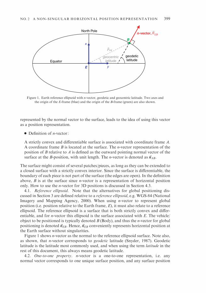
4.1. Reference ellipsoid. Note that the alternatives for global positioning dis-cussed in Section 3 are defined relative to a reference ellipsoid, e.g. WGS-84 (NationalImagery and Mapping Agency, 2000). When using n-vector to represent globalposition (i.e. position relative to the Earth frame, E), it must also relate to a referenceellipsoid. The reference ellipsoid is a surface that is both strictly convex and differ-entiable, and for n-vector this ellipsoid is the surface associated with E. The vehicle/object to be positioned is typically denoted B (Body), and thus the n-vector for globalpositioning is denoted~nnEB. Hence, ~nnEB conveniently represents horizontal position atthe Earth surface without singularities.
Figure 1 shows n-vector as the normal to the reference ellipsoid surface. Note also,as shown, that n-vector corresponds to geodetic latitude (Snyder, 1987). Geodeticlatitude is the latitude most commonly used, and when using the term latitude in therest of this document, this always means geodetic latitude.
4.2. One-to-one property. n-vector is a one-to-one representation, i.e. anynormal vector corresponds to one unique surface position, and any surface position
geodetic latitude
n-vector,
geocentriclatitude
North Pole
E y
xB
EBp
Equator
EBn
Figure 1. Earth reference ellipsoid with n-vector, geodetic and geocentric latitude. Two axes and
the origin of the E-frame (blue) and the origin of the B-frame (green) are also shown.
NO. 2 A NON-SINGULAR HORIZONTAL POSITION REPRESENTATION 399
corresponds to one unique n-vector. This one-to-one property is not held by variousother representations, such as latitude/longitude (many-to-one), roll/pitch/yaw(many-to-one) or quaternions (Zipfel, 2000) (two-to-one).
’ Note 1. If the surface is closed, any unit vector will be a valid n-vector, and thus itwill correspond to one unique position.
’ Note 2. The one-to-one property of n-vector is due to the strict convexness anddifferentiability of the associated surface :
a. If the surface had not been strictly convex, n-vector would be one-to-many.(In addition, the lack of strict convexness means that the term ‘outwardpointing’ is not defined all over the surface, and in general n-vector cannot beuniquely defined for such surfaces.)
b. If the surface had not been differentiable, n-vector would be many-to-one.
The two cases are illustrated in Figure 2.4.3. 3D positions. So far, n-vector has been used to represent a position on the
reference surface, but in the same manner as for latitude/longitude, a 3D position canbe represented by adding a height/depth parameter (above/below the nearest part ofthe reference ellipsoid surface). Mathematically, this is a very convenient combi-nation since the n-vector defines the exact direction in space where the height/depth isvalid (e.g., if we need the vector from the ellipsoid surface to a given 3D position, it issimply found as the product of n-vector and the height). When B is not at the surface,the B in~nnEB represents the horizontal position of B. As mentioned in Section 3.2, it isusually most convenient with separate horizontal and vertical position represen-tations. However, this is not the case if working with positions near1 the Earth’scentre, since the horizontal and vertical directions are not defined there.
5. n -VECTOR CALCULATIONS. We have seen that from a geometricalpoint of view ~nnEB works very well as a representation of horizontal position. The
(a) (b)
Figure 2. a. The surface is differentiable, but not strictly convex: One n-vector corresponds
to many positions. b. The surface is strictly convex, but not differentiable: Many n-vectors
correspond to one position.
1 Positions where the depth is equal to or greater than the ellipsoid radius of curvature.
400 KENNETH GADE VOL. 63
overall usefulness also depends on how easy it is to work with n-vector in practicalcalculations. In most practical calculations, n-vector is decomposed in the E-frame,i.e. nEB
E . If, for example, we want to represent the South Pole, we see from the
definition of the E-frame in Appendix A that nEEB=x100
24
35. It should also be noted
that n-vector has approximately the same direction as the position vector pEBE (see
Figure 1 where the ellipticity is exaggerated). If assuming spherical Earth, the direc-tions are equal, i.e.
nEEB=pEEB
pEEB
�� �� (1)
where | | denotes the vector length (vector 2-norm).Note that for all equations in this paper that are valid only for spherical Earth, this
is stated directly before the equation. All other equations in this paper are valid forboth ellipsoidal and spherical Earth.
5.1. Simplified notation. For the general quantities in Table 1 there are manypossible frames (such as the position of a sensor relative to a vehicle), but for globalposition, the frames are often E and B. If all positioning is relative to Earth (E) andonly one object is positioned, the subscript is redundant and can be omitted, so wecan simply use nE. This is similar to situations where it is sufficient to use only thevariables latitude and longitude (without further specification).
5.2. Converting to or from latitude and longitude. The relations between latitude/longitude and n-vector are found in this section. Note that the relations are valid forany reference ellipsoid or sphere.
Mathematically, the longitude and latitude are the first two angles of a x-y-z Eulerangle representation of the orientation of a local level frame (such as N or L, seeAppendix A) relative to E. The latitude (l) and longitude (m) have the followingdynamical intervals :
l 2 [xp=2,p=2]
m 2 (xp,p](2)
5.2.1. From latitude and longitude to n-vector. By observing simple geometry, weget the following relation:
nE=sin (l)
sin (m) � cos (l)x cos (m) � cos (l)
24
35 (3)
This equation has no singularities, i.e., one can always calculate a uniquen-vector from a set of latitude and longitude. At the poles (l=tp/2), a zerofactor, cos(l), in both the y and z components makes the actual value of the (un-defined) longitude irrelevant. It is also clear from (3) how the discontinuity of longi-tude at tp is eliminated when using n-vector, since both cos( ) and sin( ) arecontinuous for an angle going through this value. Note that the order and signs ofthe vector elements in (3) obviously depend on the choice of E-frame axes, seeAppendix A.
NO. 2 A NON-SINGULAR HORIZONTAL POSITION REPRESENTATION 401
5.2.2. From n-vector to latitude and longitude. From the geometry, we get thefollowing relations :
l=arcsin nEx� �
(4)
m=arctan nEy ,xnEz
� �(5)
where arctan(b,a) is the four quadrant version of arctan(b/a). The x, y and z sub-scripts indicate the three components of n-vector. The longitude singularity at thepoles is apparent in the arctan( ) expression, which is undefined for the input (0,0)(however, in practical programming languages, a default output is usually returnedalso in this case, making it possible to convert back to n-vector with (3) also at thepoles).
’ Implementation considerations. Equation (4) is not recommend for implemen-tation, since the arcsin( ) function is numerically inaccurate near the poles2 andalso will return imaginary results if the input should be outside t1 due to nu-merical inaccuracy. An equivalent alternative that is robust against numericalerrors is given in (6).
Note that the four quadrant arctan( , ) is used even when we know that latitude islimited to two of the quadrants (see (2)) to avoid division by zero at the poles.Because the second parameter is non-negative, this function will always returnanswers in the correct quadrants.
5.2.3. Quaternion comparison. Orientation (three degrees of freedom) is oftenrepresented by three Euler angles or three other parameters (Craig, 1989). However,all three-parameter orientation representations have singularities (Stuelplnagel,1964), and by using 4-parameter quaternions (Zipfel, 2000), the singularities areavoided. The quaternion has a restriction of unit length to ensure it only has threedegrees of freedom.
Similarly, a surface position has two degrees of freedom, and can be represented bytwo parameters with singularities, such as latitude and longitude. n-vector adds athird parameter to avoid the singularities, and also has a restriction of unit length.Converting between Euler angles and quaternions yields equations similar to (3), (4),and (5), i.e. the quaternion is found by products of sin( ) and cos( ), and the reverseequations consist of arctan( ) and arcsin( ) functions.
5.3. n-vector relations. This section includes several useful calculations involvingn-vector, illustrating its properties.
5.3.1. Horizontal and vertical parts of an arbitrary vector. Using n-vector, it iseasy to find the vertical and horizontal parts of an arbitrary vector kE,
kEvertical= nE �kE� �
nE (7)
2 The arcsin( ) is in general numerically inaccurate for calculating angles close totp/2, just as arccos( ) is
inaccurate close to zero and p. Arctan( ) is accurate for all angles.
402 KENNETH GADE VOL. 63
The horizontal part is found by subtracting the vertical part,
kEhorizontal=kEx nE �kE� �
nE (8)
5.3.2. North and east directions. Outside the poles, the (horizontal) directions ofnorth and east are often of interest. The east direction (normal to the meridian plane)is simply given by
kEeast=100
2435rnE (9)
Similarly, the north direction (normal to the transverse plane3) is given by
kEnorth=nEr100
2435rnE (10)
Since the triple cross product is associative when the first and last vectors are equal,no parentheses are needed to specify the order of operation.
The rotation matrix relating the N and E frames is useful in many calculations, andis found from (9) and (10),
REN=kEnorthkEnorth�� �� kEeast
kEeast�� �� xnE
" #(11)
5.3.3. Angular velocity of local frame. The angular velocity of a local frame L(see Appendix A) relative to E, vEL
E , is a useful quantity, for instance in a navigationsystem. From the linear velocity of B relative to E, vEB
E, and the meridian and trans-verse radius of curvature at the current height (rroc,meridian, rroc,transverse), this angularvelocity is given by
vEEL=nEr
vEEB, north
rroc,meridian+
vEEB, east
rroc, transverse
!(12)
Equation (12) is valid for an ellipsoidal Earth model, while for a spherical model, therelation is simply
vEEL=nEr
vEEB
rroc
!(13)
where rroc is the radius of curvature, i.e. Earth radius+height.5.3.4. Derivative of n-vector and height/depth. The angular velocity found in (12)
or (13) can be used directly to describe the derivative (with respect to time) of n-vector(also for elliptical Earth),
_nnE=vEELrnE (14)
The vertical part of the angular velocity vector does not affect the update of n-vector,and hence the angular velocity of any local level coordinate frame could be used
3 The transverse plane is normal to the meridian plane and contains n-vector.
NO. 2 A NON-SINGULAR HORIZONTAL POSITION REPRESENTATION 403
in (14), for instance of N (i.e. vENE ). The derivative of n-vector is useful for
instance when integrating velocity to get position as n-vector (as will be done inSection 6.5).
If integrating to get 3D position, an update of the height/depth would also beneeded. Updating height (h) is simple when knowing n-vector,
_hh=nE �vEEB (15)
5.3.5. Surface distance. If assuming spherical Earth, the surface distance (lengthof geodesic) between two positions (given by nEA
E and nEBE ), is easy to find by utilizing
the properties of the dot and cross products,
sAB=arccos nEEA �nEEB� �
�rroc=arcsin nEEArnEEB
�� ��� ��rroc
(16)
where sAB is the surface distance between A and B. For implementation, note that thearccos( ) expression is ill-conditioned for small angles, and the arcsin( ) expression isill-conditioned for angles near p/2 (and not valid above p/2). Full numerical accuracyfor all angles is achieved by combining the two expressions into an arctan( , ) ex-pression as before (see Section 5.2.2.).
5.3.6. Horizontal geographical mean. if m horizontal positions are given asn-vectors, the geographical mean, BGM, is simply given by (assuming spherical Earth)
nEEBGM=unit
Xmi=1
nEEBi
!(17)
where nEEBiis the i’th position, and ‘unit( ) ’ makes the input vector’s length/magnitude
equal to one. Equation (17) gives the exact answer for any set of global positions(except in the case where the horizontal mean is undefined, i.e. for a set of antipodalpositions, cancelling each other).
5.4. n-vector and Cartesian position vectors. In many practical calculations, thereis a need to combine global position with position differences given as Cartesianvectors (typically relative positions within a limited area). If assuming sphericalEarth, the relations are simple when using n-vector. For elliptical Earth, exact cal-culations have almost the same complexity as (geodetic) latitude and longitude, sincen-vector is also a geodetic quantity. However, such calculations can be easily handledin practice by using two general functions:
1. ‘A and B)delta position’ : Two global positions A and B are given asn-vectors (nEA
E and nEBE ) with heights. The function calculates the position
vector from A to B, pABE .
2. ‘A and delta position)B ’ : One global position is given as nEAE with height, and
a position vector to the point B is given (pABE ). The function calculates nEB
E withheight.
The implementation of the functions is described in Appendix B. It turns out thatmost calculations involving global position and local position vectors can easily besolved using these two functions (e.g. calculations involving bearing/elevation/rangefrom a sonar/radar or when an estimated error or a lever-arm should be subtractedfrom a global position).
404 KENNETH GADE VOL. 63
5.5. Using the orientation of a local coordinate frame to represent position. In (11)we saw that REN has minus n-vector as the last column, and thus this matrix containshorizontal position information. If replacing the singular N-frame with a non-singular L-frame (given in Appendix A), REL will be a non-singular position rep-resentation (also with minus n-vector as last column). REL is the matrix mentioned inSection 3.2.4., and since this matrix is often of interest in an inertial navigation system,it is also used for horizontal position representation (Savage, 2000). It has the samequalities as n-vector with respect to the pole singularities, but as a rotation matrix, ithas six extra elements with one extra degree of freedom (the wander azimuth angledescribed in Appendix A) that for most position calculations are not relevant.
6. COMPARING LATITUDE/LONGITUDE AND n-VECTOR. Thelatitude and longitude angles are Euler angles (see Section 5.2.) and they havesingularities just like any set of three Euler angles representing orientation. Fororientation, if calculations near or at the singular points might be relevant, theEuler angles are usually replaced with a quaternion or a rotation matrix, see for ex-ample (Fortescue et al., 2003), (Levine, 2000), (Phillips, 2004), or (Obaidat andPapadimitriou, 2003). The replacement is in these references motivated by the com-mon knowledge that singularities give problems, and they do not study what wouldactually happen if trying to perform calculations using a singular representationnear or at a singular point. In the following, we will demonstrate some of theseproblems by looking at some examples where we use latitude and longitude near orat a pole. Other important reasons for using n-vector, which are also importantfar away from the poles, are the ease of use, and the exact results obtained. Someexamples will focus on these properties as well.
6.1. Example 1, relative position. A common calculation is to convert positionsgiven by latitude/longitude (located within a limited area), to relative positions in alocal metric grid, often with north and east axes (e.g. when an estimated position iscompared with a measured position). In practice, such calculations often involve theequations
Dnorth= lBxlAð ÞrrocDeast= mBxmAð Þrroc cos (lC)
(18)
for two positions A and B, where lC typically is one of the involved latitudes, or anaverage.
We immediately see that the discontinuity of longitude at t180x can lead to largeerrors in (18) (but this problem can be handled by adding specific code). Problemsthat are more serious would appear if trying to use (18) near one of the poles. If thetwo latitudes were at opposite sides of a pole, the north distance would be wrong.Near a pole, the east distance in (18) will be along a clearly curved line and it will alsodepend heavily on the latitude used. If one of the positions is at the pole, the longitudeis undefined and calculating delta east is problematic. In fact, when near a pole, thenorth and east directions will vary considerably even within a limited area, and at thepolar point, the directions are undefined.
With n-vector, the vector difference is decomposed in E, with no problems for anypositions. It is found by a simple vector difference multiplied with rroc for sphericalEarth, or by the function in Section 5.4 for ellipsoidal Earth. If the delta north and
NO. 2 A NON-SINGULAR HORIZONTAL POSITION REPRESENTATION 405
east components are desired (away from the poles), the difference vector is simplymultiplied with (11).
6.2. Example 2, surface distance. A typical calculation for many applications isto find the surface distance (length of geodesic) between two horizontal positions.Even if assuming spherical Earth, calculating the great circle distance between twopositions requires several steps to find exactly from latitudes and longitudes (an ap-proximation is often found by square summing the deltas in (18)). The resultingexpression found in many books, such as (Longley et al., 2005), (Weisstein, 2003) and(Hofmann-Wellenhof et al., 2003) gives the result as an arccos expression, see firstpart of (19). However, as discussed in Section 5.2.2 an implementation finding anangle from arccos will give numerical problems for small angles. In (Sinnott, 1984) anarcsin expression accurate for small angles is found (assuming spherical Earth). Thetwo expressions for surface distance, sAB, are
sAB=arccos sin lAð Þ sin lBð Þ+ cos lAð Þ cos lBð Þ cos mAxmBð Þð Þ �rroc
If using n-vector rather than latitude/longitude, we saw from (16) that it is easy to findthe (non-singular) n-vector versions of both the arccos and arcsin expressions in (19).
6.3. Example 3, horizontal geographical mean. In several applications, it is in-teresting to find the geographical mean of multiple horizontal positions. If the pos-itions are given as latitudes/longitudes, even when assuming spherical Earth, takingthe arithmetical mean will give an answer that is only approximately correct for asmall area, away from the poles and the t180x-line. Finding the exact answer iscomplicated when using latitudes and longitudes. On the other hand, if the positionsare given as n-vectors, the geographical mean is simply given by (17).
6.4. Example 4, interpolated position. A variant of the above example is the cal-culation of an interpolated position. Using the standard formula for linear interp-olation on the latitude/longitude coordinates will not give positions that are at theshortest path (geodesic) between the two original positions. Errors will increase nearthe poles and at larger distances. In addition, positions at each side of m=t180x willgive wrong answers. With n-vector, the standard formula for interpolation gives thecorrect result for all positions.
6.5. Example 5, integrating velocity. In several applications, such as dead-reck-oning systems and simulators, the velocity of a vehicle/object is typically integrated togive global position. We shall investigate the error build-up in the integration processwhen using latitude/longitude or n-vector as the position representation.
The velocity vector to be integrated is ~vvEB, and when the vehicle position is rep-resented by latitude/longitude, it is updated using north and east velocity. These areachieved by decomposing the velocity vector in the N frame, i.e. vEB
N, and the deri-vatives of latitude and longitude can be found by (assuming spherical Earth)
_mm=vNEB, y
cos (l) �rroc
_ll=vNEB, x
rroc
(20)
406 KENNETH GADE VOL. 63
We assume correct initial position and velocity input, and thus we only study theerrors arising from the integration process itself.
6.5.1. Part 1 – Demonstrating the error effects. To visualise the error effects ap-pearing when integrating latitude/longitude close to a pole, we will use an examplewhere much error arises during few time steps. A ship such as an LCC (large crudecarrier) has low dynamics, and we assume that 1 Hz forward or backward Eulerintegration is sufficiently accurate to integrate its position. We use spherical Earthmodel in this example and first assume that the ship follows a great circle with a speedof 7.5 m/s and zero height. It passes the North Pole with a minimum distance of 10metres, as illustrated with d2 in Figure 3, and we will look at a 50 seconds interval,where there are 20 seconds (corresponding to d1) before passing at the closest dis-tance.
To investigate the drift in an algorithm, a true trajectory is needed as a reference.With spherical Earth and no vehicle turning, it is easy to calculate the true trajectoryanalytically i.e. to directly calculate an exact true position and velocity for any pointin time (we use the fact that seen from the E frame, the trajectory follows a great circle(geodesic) that is tilted relative to the meridians). The true trajectory is showntogether with the results from the Euler algorithms in Figure 4.
Looking at the upper part of Figure 4, we see that the Euler algorithms follow thetrue latitude relatively well until the pole passing. Due to the high curvature in lati-tude during the pole passing, the algorithms get an error of about t7.5 metres asshown in Figure 5 (which shows the errors converted to metres).
For longitude (Figure 4, lower part), the Euler algorithms also get problems whenthe graph starts curving, but far more serious is the error from the latitude depen-dency, see (20). The too large value in the forward Euler latitude in the last half of thepole passing causes the longitude to be increased far too much based on the velocityin (20). The opposite is true for the backward Euler method. Another weakness of thelatitude/longitude representation is the high rate of change of longitude when close tothe pole. A longitudinal error of only 0.01 metres at the closest point in the example
Longitude =0°
Longitude =±180°
d2
d1
Figure 3. View from directly above the North Pole. The trajectory (passing the pole at d2 metres
distance) is shown in solid (with an arrowhead showing the direction). Dotted straight lines:
NO. 2 A NON-SINGULAR HORIZONTAL POSITION REPRESENTATION 407
0 10 20 30 40 50
89.998
89.9985
89.999
89.9995
90
time, s
degr
ees
Latitude vs. time True trajectory
Forward EulerBackward Euler
0 10 20 30 40 50-100
0
100
Longitude vs. time
time, s
degr
ees
Figure 4. Latitude and longitude versus time. The true longitude and latitude are calculated
directly from an exact function.
0 10 20 30 40 50
-5
0
5
Latitude error in meters
time, s
met
ers Forward Euler
Backward Euler
0 10 20 30 40 50
-100
0
100
200
Longitude error in meters
time, s
met
ers
Figure 5. Error from the forward and backward Euler methods when using the latitude and
longitude representation (calculated trajectory minus true trajectory).
408 KENNETH GADE VOL. 63
corresponds to an error of about 6400 metres at the equator. Thus, small insignificantposition errors generated close to the poles are magnified by many orders of magni-tude when moving away from the pole. In the above example, the errors that aroseduring the pole-passing are magnified as shown in part 2 of Figure 5. Even withoutthese effects, small errors in the initial position, in the velocity or in the timing (sucherrors are not included in the example), would be scaled to significant levels whenincreasing the distance from the pole.6.5.1.1. Higher order integration method. Looking at the errors from forward or
backward Euler, it is tempting to try a second order integration method like thetrapezoid method. As expected, this reduces the error significantly (down to 56metres/14x in longitude), but the error is probably still too large for most appli-cations. Using a higher rate than 1 Hz also improves the result (as studied in Section6.5.2) but for any rate, we could pass the pole at a shorter distance, and the errorwould again be unacceptable. This illustrates that the fundamental problem is thesingularity of the latitude/longitude representation, and as we will see in the nextsection, replacing latitude/longitude with the non-singular n-vector is a far bettersolution than using a more complex integration method or a higher rate.6.5.1.2. Calculating position using n-vector. Updating n-vector is done using the
velocity decomposed in the E-frame, vEBE . Note that this is a more realistic and better
suited velocity input than vEBN . vEB
E can be obtained by measuring Doppler shiftfrom GPS or from underwater transponders with known position. While vEB
E has noerror due to own position error, vEB
N is decomposed in the north and east directions,and in the polar regions these directions themselves will have errors given directly bythe error in our assumed position. Combining (13) and (14) we find that the derivativeof n-vector is calculated by (assuming spherical Earth)
_nnE=nErvEEB
rroc
!rnE (21)
Note that even if the full 3D vector vEBE is used, only the horizontal component will
contribute due to the cross product with nE.Using the derivative as input, updating n-vector with the forward and
backward Euler methods gives the result shown in Figure 6. The difference fromthe true trajectory is too small to be visible in this figure, but as we did for latitudeand longitude, we can calculate the error in metres, shown in Figure 7. This is doneusing the calculated and true n-vector in (16) or by multiplying the differencevector with rroc, which gives the same result for small angles. By comparingwith Figure 5, we see that replacing latitude and longitude with n-vector has reducedthe accumulated error from ca. 228 metres (great circle error, found by using(3) and (16)) to only 2.1r10x9 metres (both numbers are the largest error fromeither the forward or backward Euler method). The latter is at the level of errorsfrom the computer’s numerical precision used in the test, i.e. IEEE 754 double pre-cision, which near the surface of the Earth gives a precision of rroc/2
52 B 1.4r10x9
metres.6.5.2. Part 2 – Sensitivity analysis. The trajectory used in Part 1 was practically
straight (only curving due to the Earth’s curvature), and thus errors arising in theEuler methods when the vehicle is turning were not included. The LCC in the exampletypically makes a heading change at 0.3x/s, and a 60x turn (simplified to follow a circle
NO. 2 A NON-SINGULAR HORIZONTAL POSITION REPRESENTATION 409
segment) will generate an error of t3.75 metres for 2D Cartesian coordinates withthe 1 Hz Euler methods. The error is not dependent on the turning rate, but on thespeed and the net number of degrees turned.
0 10 20 30 40 500
1
2
x 10-9 n-vector error in meters (in E)
time, s
x, m
eter
s
Forward Euler
Backward Euler
0 10 20 30 40 50
-1
0
1x 10
-10
time, s
y, m
eter
s
0 10 20 30 40 50
-10-505
x 10-15
time, s
z, m
eter
s
Figure 7. Error from the forward and backward Euler methods when using the n-vector
representation.
0 10 20 30 40 50
1
1
n-vector ( nE )
time, sx
True trajectory
Forward EulerBackward Euler
0 10 20 30 40 50
-2024
x 10-5
time, s
y
0 10 20 30 40 50
-1.5696-1.5696-1.5696-1.5696
x 10-6
time, s
z
Figure 6. The components of n-vector versus time. The true n-vector is calculated directly from
an exact function. (The errors of the Euler methods are too small to be visible in this plot.)
410 KENNETH GADE VOL. 63
We will now expand the scenario to start 10 minutes before the Pole passing(corresponding to d1 in Figure 3), include two 30x starboard turns and last for 1 hour,where the turns start at 15 and 30 minutes. The distance to the Pole (d2 in Figure 3)will be varied, and we will look at the final error as a function of this distance. Theresults from similar straight trajectories (i.e. no vehicle turning) are also includedfor comparison. For the straight trajectories, the true trajectory is found analyticallyas in Part 1, while for the curved trajectories the truth is found using NavLab(Gade, 2004) running at 100 Hz (NavLab uses the trapezoid method and has no polesingularities).
Figure 8 shows the result, and for the curved trajectory, the error in latitude/longitude is 4.1 metres when passing the Pole at 300 km distance, while passing at5 metres distance gives an error of about 42 km. For n-vector, the only visible error isthe expected 3.75 metres arising from the turning, independent of the distance to thePole. For the straight trajectory, we get similar results, but the error of 3.75 metresfrom the turning is removed (and the small changes in n-vector error visible in Figure8a is because the computer’s numerical precision gives different error accumulation atdifferent locations).
A common rule of thumb when considering error sources is to ignore an errorsource if it is below 10% of a known error. To reduce the extra error generated fromthe use of the latitude/longitude representation to this level, compared to the errorfrom the turning, requires a distance of about 250 km from the pole in this example.Note that in a practical application, there will be other error sources, other inte-gration periods and other dynamics, and thus the distance where the extra error fromthe latitude/longitude representation could be neglected will vary from application toapplication.6.5.2.1. Sensitivity of integration period. We could also do a sensitivity analysis by
reducing the integration period to see if this would give acceptable performance forthe 10 metres Pole distance scenario. To be able to use the analytical true trajectory,the straight trajectory from above is used. The result is shown in Figure 9 whereincreasing the rate to 100 Hz reduces the latitude/longitude error to 170 metres. Forn-vector, the higher rate first reduces the error in a similar manner, but for very highrates, the total number of iterations is considerably increased, and thus the accumu-lation of round-off errors increases the total error.
6.5.3. Conclusion. Integrating position using latitude and longitude can giveunacceptably large errors when close to a Pole, particularly due to the coupling oferror from latitude to longitude. In the given example, a distance in the order of100 km from the Pole was needed to be able to safely neglect this additional errorsource. By using n-vector instead, no additional error is introduced (the error herewas determined by the actual curvature of the trajectory or by computer precision forstraight trajectory).
6.6. Example 6. Change reference of a position vector. In many applications, anobject’s (3D) position given relative to one frame needs to be expressed relative toanother frame. For example, this calculation is needed if a vehicle position measuredby one radar should be expressed relative to a second radar. The global positions ofboth radars are given and a classical approach to this problem is to assume that eachradar has an associated N-frame. The vector to the vehicle is given relative to anddecomposed in one N-frame, and should be found relative to and decomposed in thesecond N-frame. Using the elliptical Earth model, a classical approach is based on
NO. 2 A NON-SINGULAR HORIZONTAL POSITION REPRESENTATION 411
latitude and longitude (Moore and Blair, 2000) and gives the answer using 16 lines ofcode. Solving the same problem using n-vector and the functions in Section 5.4 isintuitive, and only 4 lines of code need be written. Counting the code lines inside thefunctions used, and multiplying for repeating use of functions gives a total of 10 codelines.
(a)
(b)
0 50 100 150 200 250 300
10-8
10-6
10-4
10-2
100
102
104
Final Euler error vs. min. pole distance
pole distance, km
erro
r, m
Long/lat, curved traj.
n-vector, curved traj.Long/lat, straight traj.
n-vector, straight traj.
0 50 100 150 200 250 300
0
1
2
3
4
5
Final Euler error vs. min. pole distance
pole distance, km
erro
r, m
Long/lat, curved traj.
n-vector, curved traj.Long/lat, straight traj.
n-vector, straight traj.
Figure 8. Final error in the Euler methods (the method with the largest error is plotted) at
different distances to the pole (d2). In part a, the magnitude of the spike is compressed by using a
logarithmic scale at the y-axis. Part b is zoomed in without including the large spike and has a
linear y-axis.
412 KENNETH GADE VOL. 63
The above problem used N-frames, and is thus inherently singular at any pole.Another variant of the problem would be if the original and final vectors were givenin the radar frames (where they are measured), and the orientation was given relativeto E (which is the natural measurement from a multi-antenna GPS), rather than N.This variant is also discussed in (Moore and Blair, 2000) and in the classical solutionnew lines of code are needed for this variant (since the solution still goes via theN-frames). For n-vector, the total code now consists of only two lines, and in ad-dition, the solution is completely non-singular.
If local level frames are desired also in the polar regions, non-singular code is easilyachieved with the n-vector approach by replacing N with a non-singular frame. Forthe classical approach, this is not possible, since it is based on latitude and longitude.
7. n -VECTOR USAGE. In practice, it turns out that n-vector can be usedfor most position calculations where global position is involved. After presentingthis alternative for various research groups at FFI and collaborating universitiesand research institutes, n-vector has replaced other alternatives in numerous appli-cations. Examples of military usage include position calculations for radars, passivesubmarine sonars and active ship sonars, where the position calculations includetarget tracking. For navigation applications, n-vector is central for the position cal-culations in NavLab, HAIN (Marthiniussen et al. 2004) and the HUGIN real-timenavigation system (Hagen et al., 2003) and (Jalving et al., 2004). Applicationsinclude real-time and post-processing implementations in Matlab, C++ and C#,where thousands of hours of sensor data have been processed using n-vector, since1999.
0 20 40 60 80 100
10-10
10-8
10-6
10-4
10-2
100
102
104
Final Euler error vs. integration rate
frequency, Hz
erro
r, m
Long/lat
n-vector
Figure 9. Final error in forward or backward Euler (the one with largest error is plotted) at
different integration rates for straight trajectory, with a minimum pole distance (d2) of 10 metres.
The y-axis is logarithmic.
NO. 2 A NON-SINGULAR HORIZONTAL POSITION REPRESENTATION 413
7.1. Using n-vector for attitude representation. n-vector is usually decomposed inE for horizontal position representation. However, if n-vector is decomposed in B, itwill serve as a convenient and non-singular representation of roll and pitch. This isuseful in several situations, since roll and pitch are often treated together, separatelyfrom yaw (heading). Actually nB relates to roll and pitch, in the same way as nE relatesto latitude and longitude. Since the focus of this paper is on position representation,the treatment of nB as orientation representation will not be covered here.
8. CONCLUSIONS. Calculations involving global position often include theuse of latitude/longitude, local north/east grids or map projections. The lattertwo alternatives involve limitations and approximations, and we have seen that thelatitude/longitude representation has several complex properties, such as error inlatitude leading to error in longitude, a discontinuity at longitude=t180x, andlongitude rate going towards infinity at the poles. Numerous examples have shownthat the use of n-vector to represent horizontal position gives one or more of thefollowing advantages compared to the traditional approaches (for elliptical orspherical Earth model) :
’ There are no singularities at the poles or problems at longitude=t180x (thecode works equally well for all global positions).
’ An exact answer is returned (no approximations are made leading to increasingerrors with increasing distances).
’ Fewer lines of code are needed to solve typical position calculations.’ Implementation of the code is intuitive (no need to look up a specific procedure).’ No if-statements or iterations are needed in the code.
At FFI and collaborating universities and research institutes, n-vector has success-fully been replacing other alternatives in numerous military and civilian applicationsand commercial products since 1999.
ACKNOWLEDGEMENTS
The author would like to thank everyone that has suggested topics and improvements of thispaper, in particular scientists and engineers at the Norwegian Defence Research Establishment(FFI), the University Graduate Centre and Kongsberg Maritime.
REFERENCES
Aeronautical Systems Div Wright-Patterson AFB OH (1986). Specification for USAF Standard Form, Fit
and Function Medium Accuracy Inertial Navigation Unit (SNU-84.1).
Britting, K.R. (1971). Inertial Navigation Systems Analysis. Wiley Interscience.