A Note on MAR, Identifying Restrictions, Model Comparison, and Sensitivity Analysis in Pattern

Identification and Sensitivity Analysis in Pattern Mixture Model 1

A Note on MAR, Identifying Restrictions, Model Comparison, and Sensitivity

Analysis in Pattern Mixture Models With and Without Covariates for

Incomplete Data

Chenguang Wang

Division of Biostatistics, Center for Devices and Radiological Health, FDA, Silver Spring, Maryland 20993

email: [email protected]

and

Michael J. Daniels

Department of Statistics,University of Florida, Gainesville, FL 32611

email: [email protected]

Summary: Pattern mixture modeling is a popular approach for handling incomplete longitudinal

data. Such models are not identifiable by construction. Identifying restrictions are one approach

to mixture model identification (Little, 1995; Little and Wang, 1996; Thijs et al., 2002; Kenward

et al., 2003; Daniels and Hogan, 2008) and are a natural starting point for missing not at random

sensitivity analysis (Thijs et al., 2002; Daniels and Hogan, 2008). However, when the pattern specific

models are multivariate normal, identifying restrictions corresponding to missing at random may

not exist. Furthermore, identification strategies can be problematic in models with covariates (e.g.

baseline covariates with time-invariant coefficients). In this paper, we explore conditions necessary

for identifying restrictions that result in missing at random (MAR) to exist under a multivariate

normality assumption and strategies for identifying sensitivity parameters for sensitivity analysis or

for a fully Bayesian analysis with informative priors. In addition, we propose alternative modeling

and sensitivity analysis strategies under a less restrictive assumption for the distribution of the

observed response data. We adopt the deviance information criterion for model comparison and

perform a simulation study to evaluate the performances of the different modeling approaches.

We also apply the methods to a longitudinal clinical trial. Problems caused by baseline covariates

Biometrics 000, 000–000 DOI: 000

000 0000

with time-invariant coefficients are investigated and an alternative identifying restriction based on

residuals is proposed as a solution.

Key words: Missing at random; Non-future dependence; Deviance information criterion.

c© 0000 The Society for the Study of Evolution. All rights reserved.


1. Introduction

For analyzing longitudinal studies with informative missingness, popular modeling frame-

works include pattern mixture models, selection models and shared parameter models, which

differ in the way the joint distribution of the outcome and missing data process are factorized

(for a comprehensive review, see Little, 1995; Hogan and Laird, 1997; Kenward and Molen-

berghs, 1999; Molenberghs and Kenward, 2007; Daniels and Hogan, 2008). In this paper, we

concern ourselves with pattern mixture models with monotone missingness (i.e., drop-out).

For pattern mixture models with non-monotone (i.e., intermittent) missingness (details go

beyond the scope of this paper), one approach is to partition the missing data and allow one

(or more) or the partitions to be ignored given the other partition(s) (Harel and Schafer,

2009; Wang et al., 2010).

It is well known that pattern-mixture models are not identified: the observed data does not

provide enough information to identify the distributions for incomplete patterns. The use

of identifying restrictions that equate the inestimable parameters to functions of estimable

parameters is an approach to resolve the problem (Little, 1995; Little and Wang, 1996; Thijs

et al., 2002; Kenward et al., 2003; Daniels and Hogan, 2008). Common identifying restrictions

include complete case missing value (CCMV) constraints and available case missing value

(ACMV) constraints. Molenberghs et al. (1998) proved that for discrete time points and

monotone missingness, the ACMV constraint is equivalent to missing at random (MAR),

as defined by Rubin (1976) and Little and Rubin (1987). A key and attractive feature of

identifying restrictions is that they do not impact the fit of the model to the observed data.

Understanding (identifying) restrictions that lead to MAR is an important first step for

sensitivity analysis under missing not at random (MNAR) (Scharfstein et al., 2003; Zhang

and Heitjan, 2006; Daniels and Hogan, 2008). In particular, MAR provides a good starting

2 Biometrics, 000 0000

point for sensitivity analyses and sensitivity analyses are essential for inference on incomplete

data (Scharfstein et al., 1999; Vansteelandt et al., 2006; Daniels and Hogan, 2008).

The normality of response data (if appropriate) for pattern mixture models is desirable as

it easily allows incorporation of baseline covariates and introduction of sensitivity parame-

ters (for MNAR analysis) that have convenient interpretations as deviations of means and

variances from MAR (Daniels and Hogan, 2008). However, multivariate normality within

patterns can be overly restrictive. We explore such issues in this paper.

One criticism of mixture models is that they often induce missing data mechanisms that

depend on the future (Kenward et al., 2003). We explore such non-future dependence in our

context here and show how mixture models that have such missing data mechanisms have

fewer sensitivity parameters.

In Section 2, we show conditions under which MAR exists and does not exist when the

full-data response is assumed multivariate normal within each missing pattern. In Section 3

and Section 4 in the same setting, we explore sensitivity analysis strategies under MNAR

and under non-future dependent MNAR respectively. In Section 5, we propose a sensitivity

analysis approach where only the observed data within pattern are assumed multivariate

normal. In Section 6, we apply the frameworks described in previous sections to a randomized

clinical trial for estimating the effectiveness of recombinant growth hormone for increasing

muscle strength in the elderly and propose a criterion to compare the fit of different models

to the observed data. The behavior of this criterion and the model frameworks proposed

in Sections ??-5 are assessed by simulation in Section 7. In Section 8, we show that in

the presence of baseline covariates with time-invariant coefficients, standard identifying

restrictions cause over-identification of the baseline covariate effects and we propose a remedy.

We provide conclusions and discussion in Section 9.


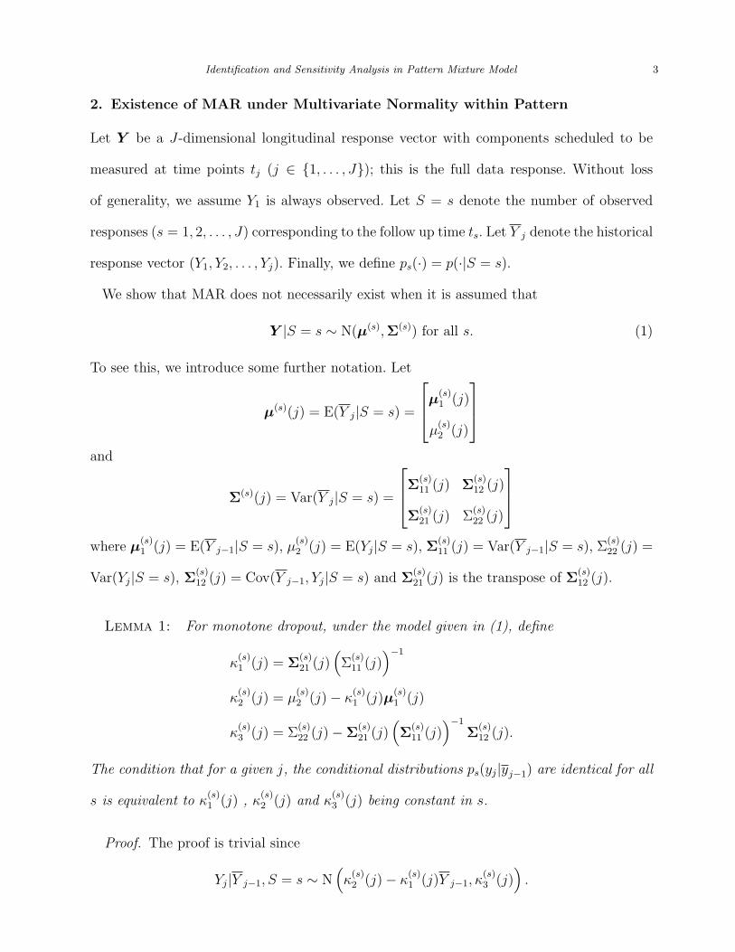
2. Existence of MAR under Multivariate Normality within Pattern

Let Y be a J-dimensional longitudinal response vector with components scheduled to be

measured at time points tj (j ∈ {1, . . . , J}); this is the full data response. Without loss

of generality, we assume Y1 is always observed. Let S = s denote the number of observed

responses (s = 1, 2, . . . , J) corresponding to the follow up time ts. Let Y j denote the historical

response vector (Y1, Y2, . . . , Yj). Finally, we define ps(·) = p(·|S = s).

We show that MAR does not necessarily exist when it is assumed that

Y |S = s ∼ N(µ(s),Σ(s)) for all s. (1)

To see this, we introduce some further notation. Let

µ(s)(j) = E(Y j|S = s) =

µ(s)1 (j)

µ(s)2 (j)

and

Σ(s)(j) = Var(Y j|S = s) =

Σ(s)11 (j) Σ

(s)12 (j)

Σ(s)21 (j) Σ

(s)22 (j)

where µ

(s)1 (j) = E(Y j−1|S = s), µ

(s)2 (j) = E(Yj|S = s), Σ

(s)11 (j) = Var(Y j−1|S = s), Σ

(s)22 (j) =

Var(Yj|S = s), Σ(s)12 (j) = Cov(Y j−1, Yj|S = s) and Σ

(s)21 (j) is the transpose of Σ

(s)12 (j).

Lemma 1: For monotone dropout, under the model given in (1), define

κ(s)1 (j) = Σ

(s)21 (j)

(Σ

(s)11 (j)

)−1

κ(s)2 (j) = µ

(s)2 (j)− κ

(s)1 (j)µ

(s)1 (j)

κ(s)3 (j) = Σ

(s)22 (j)−Σ

(s)21 (j)

(Σ

(s)11 (j)

)−1

Σ(s)12 (j).

The condition that for a given j, the conditional distributions ps(yj|yj−1) are identical for all

s is equivalent to κ(s)1 (j) , κ

(s)2 (j) and κ

(s)3 (j) being constant in s.

Proof. The proof is trivial since

Yj|Y j−1, S = s ∼ N(κ

(s)2 (j)− κ

(s)1 (j)Y j−1, κ

(s)3 (j)

).


In other words, if the condition in Lemma 1 is satisfied, then there exists a conditional

distribution p≥s(yj|yj−1) such that ps(yj|yj−1) = p≥s(yj|yj−1) for all s ≥ j. We now state a

theorem that gives the restrictions on the model given in (1) for MAR to exist. Note that

the proofs of rest of the theorems and corollaries in this and the subsequent section can be

found in Web Appendix A.

Theorem 1: For pattern mixture models with monotone dropout, under the model given

in (1), identification via MAR constraints exists if and only if µ(s) and Σ(s) satisfy Lemma

1 for s ≥ j and 1 < j < J .

So, a default approach for continuous Y , assuming the full data response is multivariate nor-

mal within pattern, does not allow an MAR restriction (unless the restrictions in Theorem 1

are imposed).

We now examine the corresponding missing data mechanism (MDM), S|Y . We use “'”

to denote equality in distribution.

Corollary 1: For pattern mixture models of the form (1) with monotone dropout, MAR

holds if and only if S|Y ' S|Y1.

Thus, the implicit MDM is very restrictive and does not depend on the entire history, Y s.

We now show connections to missing completely at random (MCAR) and other common

identifying restrictions.

Corollary 2: For pattern mixture models of the form (1) with monotone dropout,

MCAR is equivalent to MAR if ps(y1) = p(y1) for all s.



MAR constraints are identical to complete case missing value (CCMV) and nearest-neighbor

constraints (NCMV).

The results in this section were all based on specifying the mixture model in (1) and

demonstrate that MAR only exists under the fairly strict conditions given in Theorem 1.

3. Sequential Model Specification and Sensitivity Analysis under MAR

Due to the structure of µ(s) and Σ(s) under MAR constraints as outlined in Section 2,

we propose to follow the approach in Daniels and Hogan (2008, Chapter 8) and specify

distributions of observed Y within pattern as:

ps(y1) ∼ N(µ(s)1 , σ

(s)1 ) 1 ≤ s ≤ J

ps(yj|yj−1) ∼ N(µ(≥j)

j|j− , σ(≥j)

j|j− ) 2 ≤ j ≤ s ≤ J

(2)

where j− = {1, 2, . . . , j − 1}. Note that by construction, we assume ps(yj|yj−1) are identical

for all j ≤ s ≤ J . Consequently, we have ps(yj|yj−1) = p(yj|yj−1, S ≥ s), denoted as

p≥s(yj|yj−1).


identification via MAR constraints exists if and only if the observed data can be modeled

as (2).

Corollary 4 implies that under the multivariate normality assumption in (1) and the MAR

assumption, a sequential specification as in (2) always exists.

We provide some details for MAR in model (1) (which implies the specification in (2) as

stated in Corollary 4) next. Distributions for missing data (which are not identified) are

specified as:

ps(yj|yj−1) ∼ N(µ(j)

j|j− , σ(j)

j|j−) 1 ≤ s < j ≤ J.


The conditional mean structure of µ(≥j)

j|j− and µ(j)

j|j− is parameterized as follows:

µ(≥j)

j|j− = β(≥j)0 +

j−1∑l=1

β(≥j)l yl

µ(j)

j|j− = β(j)0 +

j−1∑l=1

β(j)l yl.

To identify the full-data model, the MAR constraints require that

pk(yj|yj−1) = p≥j(yj|yj−1)

for k < j, which implies that µ(j)

j|j− = µ(≥j)

j|j− and σ(j)

j|j− = σ(≥j)

j|j− for 2 ≤ j ≤ J . Since the

equality of the conditional means need to hold for all Y , this further implies that the MAR

assumption requires that β(j)l = β

(≥j)l , 0 ≤ l < j ≤ J .

The motivation of the proposed sequential model is to allow a straightforward extension of

the MAR specification to a large class of MNAR models indexed by parameters measuring

departures from MAR, as well as the attraction of doing sensitivity analysis on means and/or

variances in normal models.

For example, we can let

β(j)l = ∆

(j)l + β

(≥j)l and log σ

(j)

j|j− = ∆(j)σ + log σ

(≥j)

j|j−

for all j > 1 and 0 ≤ l < j. Sensitivity analysis can be done on these ∆ parameters that

capture the information about the missing data mechanism (see Web Appendix B for the

impact of the ∆ parameters on the MDM). For example, in a Bayesian framework, we may

assign informative priors elicited from experts to these sensitivity parameters ∆. Note in

general we may have separate ∆(j)l and ∆

(j)σ for each pattern s (s ≤ j), but in practice it is

necessary to limit the dimensionality of these (Daniels and Hogan, 2008). Indeed, we could

make ∆(j)l and ∆

(j)σ independent of j to further reduce the number of sensitivity parameters.

In general the MDM depends on Y J , i.e. MNAR, in presence of the the ∆ parameters.

However, one might want hazard at time ts to only depend on Y s+1, in which case we need


to have different distributions and assumptions on [Yj|Y j−1, S = k] for k < j − 1 and j > 2,

as shown in the next section.

4. Non-future Dependence and Sensitivity Analysis under Multivariate

Normality within Pattern

Non-future dependence assumes that missingness only depends on observed data and the

current missing value, i.e.

[S = s|Y ] ' [S = s|Y s+1],

and can be viewed as a special case of MNAR and an extension of MAR (Kenward et al.,

2003). Kenward et al. (2003) showed that non-future dependence holds if and only if for each

j ≥ 3 and k < j − 1,

pk(yj|yj−1) = p≥j−1(yj|yj−1).

An approach to implement non-future dependence within the framework of Section 3 is as

follows. We model the observed data as in (2). For the conditional distribution of the current

missing data (Ys+1), we assume that

ps(ys+1|ys) ∼ N

(β

(≥s+1)0 + ∆

(s+1)0 +

s∑l=1

(β(≥s+1)l + ∆

(s+1)l )yl, e

∆(s+1)σ σ

(≥s+1)

s|s−

)2 ≤ s < J

and for the conditional distribution of the future missing data (Ys+2, . . . , YJ), we assume that

ps(yj|yj−1) = p≥j−1(yj|yj−1) 2 ≤ s < j − 1 ≤ J − 1,

where

p≥j−1(yj|yj−1) =p(S = j − 1)

p(S ≥ j − 1)pj−1(yj|yj−1) +

p(S ≥ j)

p(S ≥ j − 1)p≥j(yj|yj−1).

Note that by this approach, although the model for future missing data is a mixture

of normals, the sensitivity parameters are kept the same as in Section 3 (∆(j)l and ∆

(j)σ ,

j = 2, . . . , J and l = 0, . . . , j − 1). In addition, this significantly reduces the number of

potential sensitivity parameters. For J-dimensional longitudinal data, the total number of


sensitivity parameters, (2J3 + 3J2 + J)/6 − J is reduced to (J2 + 3J − 4)/2; for J=3 (6),

from 11 (85) to 7 (25). Further reduction is typically needed. See the data example in

Section 6 as an illustration. If all of the remaining sensitivity parameters are set to zero,

we have ps(ys+1|ys) = p≥s+1(ys+1|ys) for 2 ≤ s < J and ps(yj|yj−1) = p≥j(yj|yj−1) for

2 ≤ s < j − 1 ≤ J − 1, which implies ps(yj|yj−1) = p≥j(yj|yj−1) for all s < j, i.e. MAR.

5. MAR and Sensitivity Analysis with Multivariate Normality on the

Observed-data Response

If we assume multivariate normality only on observed data response, Y obs|S instead of the

full data response, Y |S, we can weaken the restrictions on ps(yj|yj−1) for s ≥ j and allow

the MDM to incorporate all observed data under MAR (cf. Corollary 1).

For example, we may specify distributions Y obs|S as follows:

ps(y1) ∼ N(µ(s)1 , σ

(s)1 ) 1 ≤ s ≤ J

ps(yj|yj−1) ∼ N(µ(s)

j|j− , σ(s)

j|j−) 2 ≤ j ≤ s ≤ J

where

µ(s)

j|j− = β(s)j,0 +

j−1∑l=1

β(s)j,l Yl.

To identify the full-data model, recall the MAR constraints imply that

ps(yj|yj−1) = p≥j(yj|yj−1) =J∑

k=j

P (S = k)

P (S ≥ j)pk(yj|yj−1) (3)

for s < j, which are mixture of normals. For sensitivity analysis in this setting of mixture of

normals, we propose to introduce sensitivity parameters ∆µ (location) and ∆σ (scale) such

that for s < j

ps(yj|yj−1) = e−∆(j)σ

J∑k=j

$j,kpk(yj −∆

(j)µ − (1− e∆

(j)σ )µ

(k)j|j−

e∆(j)σ

∣∣yj−1) (4)

where $j,k = P (S=k)P (S≥j)

. The rationale for this parameterization is that each pk(·|yj−1) in the

summation will have mean ∆(j)µ +µ

(k)j|j− and variance e2∆

(j)σ σ

(k)j|j−1. To reduce the dimension of


the sensitivity parameters, we could make ∆(j)µ and ∆

(j)σ common for all j (namely ∆µ and

∆σ).

In this set up, we have

µ(s),MNARj|j− = ∆(j)

µ +J∑

k=j

$j,kµ(k)j|j−

and

σ(s),MNARj|j− = e2∆

(j)σ

J∑

k=j

$j,k

(σ

(k)j|j−1 + (µ

(k)j|j−1)

2)−

(J∑

k=j

$j,kµ(k)j|j−

)2+ (1− e2∆

(j)σ )M

where

M =J∑

k=j

$j,k(µ(k)j|j−)2 −

(J∑

k=j

$j,kµ(k)j|j−

)2

(see Web Appendix C for details). Note that M does not depend on σ(k)j|j−1 for k = j, . . . , J .

Under an MAR assumption (3), for [Yj|Y j−1, S = s], we have

µ(s),MARj|j− =

J∑k=j

$j,kµ(k)j|j−

and

σ(s),MARj|j− =

J∑k=j

$j,k

(σ

(k)j|j−1 + (µ

(k)j|j−1)

2)− (µ

(s),MARj|j− )2.

Therefore, under MNAR assumption (4), the two sensitivity parameters control the departure

of the mean and variance from MAR in the following way,

µ(s),MNARj|j− = ∆(j)

µ + µ(s),MARj|j− and σ

(s),MNARj|j− = e2∆

(j)σ σ

(s),MARj|j− + (1− e2∆

(j)σ )M ,

with ∆(j)µ being a location parameter and ∆

(j)σ being a scale parameter. The MNAR class

allows MAR when ∆(j)µ = ∆

(j)σ = 0 for all j ≥ 2.

By assuming non-future dependence, we obtain

ps(yj|yj−1) = p≥j−1(yj|yj−1) =p(S = j − 1)

p(S ≥ j − 1)e−∆

(j)σ

J∑k=j

$j,kpk(yj −∆

(j)µ − (1− e∆

(j)σ )µ

(k)j|j−

e∆(j)σ

|yj−1)

+J∑

k=j

P (S = k)

p(S ≥ j − 1)pk(yj|yj−1) 2 ≤ s < j − 1 ≤ J − 1,

for the future data and (4) for the current data (j = s + 1). The number of sensitivity


parameters in this setup is reduced from J(J−1) by (J−2)(J−1) to 2(J−1); so, for J = 3

(6), from 6 (30) to 2 (20). Further reductions are illustrated in Section 6.

6. Example: Growth Hormone Study

We analyze a longitudinal clinical trial using the framework from Sections 4 and 5 that

assume multivariate normality for the full-data response within pattern (MVN) or multi-

variate normality for the observed data response within pattern (OMVN). We assume non-

future dependence for the missing data mechanism to minimize the number of sensitivity

parameters.

The growth hormone (GH) trial was a randomized clinical trial conducted to estimate the

effectiveness of recombinant human growth hormone therapy for increasing muscle strength

in the elderly. The trial had four treatment arms: placebo (P), growth hormone only (G),

exercise plus placebo (EP), and exercise plus growth hormone (EG). Muscle strength, here

mean quadriceps strength (QS), measured as the maximum foot-pounds of torque that can

be exerted against resistance provided by a mechanical device, was measured at baseline, 6

months and 12 months. There were 161 participants enrolled on this study, but only (roughly)

75% of them completed the 12 month follow up. Researchers believed that dropout was

related to the unobserved strength measures at the dropout times.

For illustration, we confine our attention to the two arms using exercise: exercise plus

growth hormone (EG) and exercise plus placebo (EP). Table 1 contains the observed data

for the two arms.

[Table 1 about here.]

Let (Y1, Y2, Y3) denote the full-data response corresponding to baseline, 6 months, and

12 months. Let Z be the treatment indicator (1 = EG, 0 = EP). Our goal is to draw

inference about the mean difference of QS between the two treatment arms at month 12.


That is, the treatment effect θ = E(Y3|Z = 1) − E(Y3|Z = 0). In the full-data model

for each treatment under non-future dependence, there are seven sensitivity parameters for

the MVN model: {∆(2)0 , ∆

(2)1 , ∆

(3)0 , ∆

(3)1 , ∆

(3)2 , ∆

(2)σ , ∆

(3)σ }, and four sensitivity parameters for

OMVN model: {∆(2)µ , ∆

(3)µ , ∆

(2)σ , ∆

(3)σ }; see Web Appendix D for details on the models. For

the MNAR analysis, we reduced the number of sensitivity parameters as follows:

• ∆(2)σ and ∆

(3)σ do not appear in the posterior distribution of E(Y3|Z) for Z = 0, 1, and thus

are not necessary for inference on θ.

• We restrict to MNAR departures from MAR in terms of the intercept terms by assuming

∆(2)1 = ∆

(3)1 = ∆

(3)2 ≡ 0.

• We assume the sensitivity parameters are identical between treatments.

This reduces the set of sensitivity parameters to {∆(2)0 , ∆

(3)0 } for MVN model and {∆(2)

µ , ∆(3)µ }

for the OMVN model.

There are a variety of ways to specify priors for the sensitivity parameters ∆(2)0 and ∆

(3)0 ,

∆(2)0 = E(Y2|Y1, S = 1)− E(Y2|Y1, S ≥ 2)

∆(3)0 = E(Y3|Y2, Y1, S = 2)− E(Y3|Y2, Y1, S = 3).

Both represent the difference of conditional means between the observed and unobserved

responses. ∆(2)µ and ∆

(3)µ have (roughly) the same interpretation as ∆

(2)0 and ∆

(3)0 .

Based on discussion with investigators, we made the assumption that dropouts do worse

than completers; thus, we restrict the ∆’s to be less than or equal to zero. To do a fully

Bayesian analysis to fairly characterize the uncertainty associated with the missing data

mechanism, we assume a uniform prior for the ∆’s as a default choice. Subject matter

considerations gave an upper bound of zero for the uniform distributions. We set the lower

bound using the variability of the observed data as follows. We estimate the residual variances

of Y2|Y1 and Y3|Y2, Y1 using the observed data; we denote these by τ2|1 and τ3|2,1 respectively.

We use the square root of these estimates as the lower bounds. In particular, we specify the


priors for {∆(2)0 , ∆

(3)0 } as well as {∆(2)

µ , ∆(3)µ } as Unif(D(τ )), where

D(τ ) =[−τ

−1/22|1 , 0

]×[−τ

−1/23|2,1 , 0

]. (5)

Based on the estimates τ−1/22|1 = 18 and τ

−1/23|2,1 = 12, the priors are [−18, 0] × [−12, 0] for

{∆(2)0 , ∆

(3)0 } and for {∆(2)

µ , ∆(3)µ }. For the other parameters in the full-data model, we assign

N(0, 106) for mean parameters (µ, β) and Unif(0, 100) for variance parameters (σ1/2).

We fit the model using WinBUGS, with multiple chains of 25, 000 iterations and 4000 burn-in.

Convergence was checked by examining trace plots of the multiple chains.

The results of the MVN and OMVN models are given in Table 2. Under MNAR, the

posterior mean (posterior standard deviation) of the difference in quadriceps strength at 12

months between the two treatment arms was 4.0 (8.9) and 4.4 (10) for the MVN and OMVN

models. Under MAR the differences were 5.4 (8.8) and 5.8 (9.9) for the MVN and OMVN

models, respectively. The smaller differences under MNAR were due to quadriceps strength

at 12 months being lower under MNAR due to the assumption that dropouts do worse than

completers.

To compare the fit of models OMVN and MVN, we used the deviance information criterion

that is based on the observed data likelihood (DICO),

DICO = −4E{log L(θ|yobs, S)}+ 2 log L{E(θ|yobs, S)|yobs, S}. (6)

The results favored the OMVN model (Table 2). The behavior of DICO for model selection

in the setting of incomplete data is explored in Section 7. Note that given the OMVN or

MVN specification for the observed data, the fit (as measured by the DICO) was equivalent

across the different missingness mechanisms as it should be since the observed data provide

no information about this. We conclude that the treatment difference, θ was not significantly

different from zero.



To assess the sensitivity of the informative priors Unif(D(τ )), we evaluated several sce-

narios by making the priors more or less informative by modifying the range (see Table 3).

Specifically, we considered (1) D(τ ) = [−20, 0] × [−20, 0], (2) D(τ ) = [−9, 0] × [−6, 0], (3)

D(τ ) = [−20, 0]× [−6, 0] and (4) D(τ ) = [−9, 0]× [−20, 0]; note that the lower bounds of −9

and −6 are −τ−1/22|1 /2 and −τ

−1/23|2,1 /2, respectively. Based on subject matter considerations,

we assumed the difference of the conditional means between the observed and unobserved

responses did not exceed 20 foot pounds of torque. None of the scenarios considered resulted

in a significant mean treatment difference at month 12.


7. Model Comparison and Simulations

Although the specification in Section 3-4 arguably offers a simpler sensitivity analysis than

that in Section 5, the former may not fit the observed data as well (as indicated by DICO

in Section 6). In addition, if the conclusions between OMVN and MVN were substantially

different (unlike in the example here), we would need to decide which model to use for

inference.

Spiegelhalter et al. (2002) developed the deviance information criterion (DIC) for Bayesian

model comparison. In the setting of incomplete data, many alternative representations of

DIC have been proposed (Celeux et al., 2006; Daniels and Hogan, 2008). The underlying

complication is the fact that we do not observe the full data. Recommendations in Celeux

et al. (2006) were based on missing data that were actually latent variables in random effects

and mixture models, not potentially observable missing data as is our focus. Daniels and

Hogan (2008) recommended DICO (6) on intuitive grounds but did no exploration of its

operating characteristics. The following simulation study explores the behavior of DICO, as

well as the behavior of MVN and OMVN models.


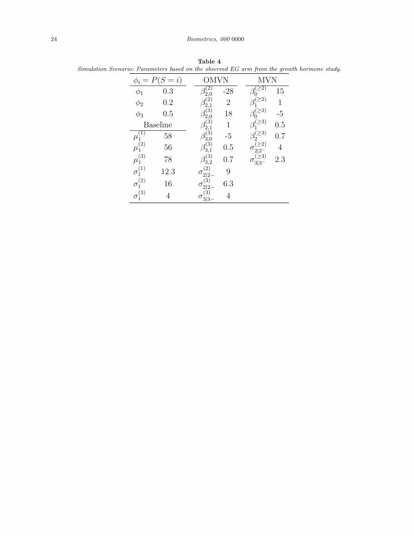
We simulated observed data from the MVN and OMVN models. Parameters estimated by

fitting the MVN and OMVN models to the observed EG arm data from the growth hormone

study were the basis for the simulation (see Table 4).


For each sample size, 50, 150 and 300, we simulated 500 datasets for MVN and OMVN

observed data models. The performance of the different approaches were assessed using both

the DICO and the mean squared error (MSE) of E(Yj) : j = 2, 3; see Table 5. Note that

we computed the “true” E(Y2) and E(Y3) for MNAR cases using the uniform prior with

D(τ ) = [−18, 0]× [−12, 0] from Section 6. For reference, the MSE’s associated with the true

data generating model are bolded.

The simulations favored the correctly specified model with respect to both DICO and MSE.

As the sample size was increased, the MSE’s decreased and the difference between the correct

and the incorrect models increased. The MSE for E[Yj] : j = 2, 3 provides information on

the fit to the full data response model (both the observed and missing data), not just the

observed data model; however, all that can be checked from the observed data is the fit to the

observed data response model. Based on this (limited) simulation, we conclude that DICO

is a reasonable criterion to choose between different incomplete data models and has more

power when the sample size is moderate or large. Sensitivity analysis and all inferences can

then be conducted on the model that fits the observed data the best. The simulation result

also showed that when the MVN specification is true, OMVN is competitive, but not vice

versa. This is reasonable because OMVN is the conservative choice here given that MVN is

nested within it.

To compare the robustness of the MVN and OMVN models when neither is correct, we

considered selection models where the distribution of Y is heavy-tailed or asymmetric.

Specifically, we simulated response data from a multivariate t (MVT) distribution Y ∼


MVT(µ,Σ, df) with df being the degrees of freedom, and a multivariate skew-normal (MSKN)

distribution Y ∼ MSKN(µ,Σ, ω) with ω being the skewness factor (Azzalini and Valle,

1996). See Web Appendix E for details of data generation for these cases.

The average DICO are reported in Table 6. Note that MAR and MNAR cases correspond

to different observed data models in this simulation setting. Therefore, we report DICO for

MAR and MNAR separately.

From the simulation, we can see that MVN model is more likely to be selected by DICO

when sample size is small. When sample size is moderate or large, OMVN model fits the

observed data better for all the cases considered and offers more robustness (in particular

for the heavy-tailed scenario). OMVN appears to be the better default choice for medium to

large sample sizes.



8. ACMV Restrictions and Multivariate Normality with Baseline Covariates

In this section, we show that common identifying restrictions over-identify estimable pa-

rameters in the presence of baseline covariates with time invariant coefficients and offer a

solution.

Consider the situation when Y = (Y1, Y2) is a bivariate normal response (J = 2) with

missing data only in Y2, i.e. S = 1 or 2. Assume there are baseline covariates X with time

invariant coefficients α. We model p(S) and p(Y |S) as follows:

S|X ∼ Bern(φ(X))

Y |S = s ∼ N(µ(s)(X),Σ(s)) s = 1, 2


where

µ(s) =

µ(s)1 + Xα(s)

µ(s)2 + Xα(s)

and Σ(s) =

σ(s)11 σ

(s)12

σ(s)21 σ

(s)22

.

MAR (ACMV) implies the following restriction

[Y2|Y1, S = 1] ' [Y2|Y1, S = 2] .

This implies that conditional means, E(Y2|Y1, X, S = s) for s = 1, 2, are equal, i.e.

µ(1)2 + Xα(1) +

σ(1)21

σ(1)11

(Y1 − µ(1)1 −Xα(1)) = µ

(2)2 + Xα(2) +

σ(2)21

σ(2)11

(Y1 − µ(2)1 −Xα(2)). (7)

For (7) to hold for all Y1 and X, we need that

α(1) = α(2).

However, both α(1) and α(2) are already identified by the observed data Y1. Thus the ACMV

(MAR) restriction affects the model fit to the observed data. This is against the principle of

applying identifying restrictions (Little and Wang, 1996; Daniels and Wang, 2009).

To resolve the over-identification issue , we propose to apply MAR constraints on residuals

instead of directly on the responses. In the bivariate case, the corresponding restriction is[Y2 −Xα(1)|Y1 −Xα(1), X, S = 1

]'[Y2 −Xα(2)|Y1 −Xα(2), X, S = 2

]. (8)

Since the conditional distributions[Y2 −Xα(s)|Y1 −Xα(s), X, S = s

]∼ N

(µ

(s)2 +

σ(s)21

σ(s)11

(Y1 − µ(s)1 ), σ

(s)22 −

(σ(s)21 )2

σ(s)11

)are independent of α(s) for s = 1, 2, the restriction (8) places no constraints on α(s), thus

avoiding over-identification.

The MDM corresponding to the ACMV(MAR) on the residuals is given by

logP (S = 1|Y , X)

P (S = 2|Y , X)= log

φ(X)

1− φ(X)− 1

2σ∗

{(1−B)2X(α(2)α(2)T − α(1)α(1)T )XT

− 2(1−B)(Y2 −∆(Y1))X(α(2) − α(1))

}− 1

2log

σ(2)11

σ(1)11

− (Y1 −Xα(2) − µ(2)1 )2

2(σ(2)11 )2

+(Y1 −Xα(1) − µ

(1)1 )2

2(σ(1)11 )2

,


where σ∗ = σ(2)22 − (σ

(2)21 )2

σ(2)11

, B =σ

(1)21

σ(1)11

and ∆(Y1) = µ(2)2 +

σ(2)21

σ(2)11

(Y1 − µ(2)1 ). Hence by assuming

MAR on the residuals, we have the MDM being a quadratic form of Y1, but independent

of Y2 if and only if α(2) = α(1). In other words, assumption (8) implies MAR if and only if

α(2) = α(1). So in general, MAR on residuals does not imply that missingness in Y2 is MAR.

However, it is an identifying restriction that does not impact the fit of the model to the

observed data. CCMV and NCMV restrictions can be applied similarly to the residuals.

Remark: In general, µ(s)l can be replaced by µ

(s)il if there are subject-specific covariates

with time varying coefficients.

The ACMV (MAR) on the residuals restriction can be applied to the multivariate case

and results in a similar MDM. Detailed discussion is provided in Web Appendix F.

9. Summary

Most pattern mixture models allow the missingness to be MNAR, with MAR as a unique

point in the parameter space. The magnitude of departure from MAR can be quantified via a

set of sensitivity parameters. For MNAR analysis, it is critical to find scientifically meaningful

and dimensionally tractable sensitivity parameters. For this purpose, (multivariate) normal

distributions are often found attractive since the MNAR departure from MAR can be

parsimoniously defined by deviations in the mean and (co-)variance.

However, a simple pattern mixture model based on multivariate normality for the full data

response within patterns does not allow MAR without special restrictions that themselves,

induce a very restrictive missing data mechanism. We have explored this fully and proposed

alternatives based on multivariate normality for the observed data response within patterns.

In both these contexts, we proposed strategies for specifying sensitivity parameters.

The proposed modeling and sensitivity analysis approaches based on within-pattern mul-

tivariate normality for the full data response or the observed data response may lead to


contradicting study conclusions, due to the different (unverifiable) missing data mechanism

assumptions and the different observed data model. For the latter, we proposed to use the

deviance information criterion that is based on the observed data likelihood for model com-

parison and selection and showed via simulations that it appears to perform well. Sensitivity

analysis and inferences can then be based upon the model that fits the observed data the

best.

In addition, we showed that when introducing baseline covariates with time invariant

coefficients, standard identifying restrictions result in over-identification of the model. This

is against the principle of applying identifying restriction in that they should not affect the

model fit to the observed data. We proposed a simple alternative set of restrictions based on

residuals that can be used as an ’identification’ starting point for an analysis using mixture

models.

In the growth hormone study data example, we showed how to reduce the number of

sensitivity parameters in practice and a default way to construct informative priors for sen-

sitivity parameters based on limited knowledge about the missingness. In particular, all the

values in the range D were weighted equally via a uniform distribution. If there is additional

external information from expert opinion or historical data, informative priors may be used to

incorporate such information (for example, see Ibrahim and Chen, 2000; Wang et al., 2010).

Finally, an important consideration in sensitivity analysis and constructing informative priors

is that they should avoid extrapolating missing values outside of a reasonable range (e.g.,

in the growth hormone trial example, we would not want to impute a negative quadriceps

strength).

10. Supplementary Materials

Web Appendices and Tables referenced in Sections 2, 3, 5, 6, 7, and 8 are available under

the Paper Information link at the Biometrics website http://www.biometrics.tibs.org.


Acknowledgment

This research was supported by NIH grants CA-85295 and HL-079457.

References

Azzalini, A. and Valle, A. (1996). The multivariate skew-normal distribution. Biometrika

83, 715–726.

Celeux, G., Forbes, F., Robert, C., and Titterington, D. (2006). Deviance information criteria

for missing data models. Bayesian Analysis 1, 651–674.

Daniels, M. and Hogan, J. (2008). Missing Data in Longitudinal Studies: Strategies for

Bayesian Modeling and Sensitivity Analysis. Chapman & Hall/CRC.

Daniels, M. and Wang, C. (2009). Discussion of “Missing Data in longitudinal studies: A

review” by Ibrahim and Molenberghs. TEST 18, 51–58.

Harel, O. and Schafer, J. (2009). Partial and latent ignorability in missing-data problems.

Biometrika 96, 37.

Hogan, J. and Laird, N. (1997). Model-based approaches to analysing incomplete longitudinal

and failure time data. Statistics in Medicine 16, 259–272.

Ibrahim, J. and Chen, M. (2000). Power prior distributions for regression models. Statistical

Science 15, 46–60.

Kenward, M. and Molenberghs, G. (1999). Parametric Models for Incomplete Continuous

and Categorical Longitudinal Data. Statistical Methods in Medical Research 8, 51.

Kenward, M., Molenberghs, G., and Thijs, H. (2003). Pattern-mixture models with proper

time dependence. Biometrika 90, 53–71.

Little, R. (1995). Modeling the drop-out mechanism in repeated-measures studies. Journal

of the American Statistical Association 90,.

Little, R. and Rubin, D. (1987). Statistical Analysis with Missing Data. Wiley.


Little, R. and Wang, Y. (1996). Pattern-mixture models for multivariate incomplete data

with covariates. Biometrics 52, 98–111.

Molenberghs, G. and Kenward, M. (2007). Missing Data in Clinical Studies. Wiley.

Molenberghs, G., Michiels, B., Kenward, M., and Diggle, P. (1998). Monotone Missing Data

and Pattern-Mixture Models. Statistica Neerlandica 52, 153–161.

Rubin, D. (1976). Inference and missing data. Biometrika 63, 581–592.

Scharfstein, D., Daniels, M., and Robins, J. (2003). Incorporating Prior Beliefs about Selec-

tion Bias into the Analysis of Randomized Trials with Missing Outcomes. Biostatistics

4, 495.

Scharfstein, D., Rotnitzky, A., and Robins, J. (1999). Adjusting for Nonignorable Drop-

Out Using Semiparametric Nonresponse Models. Journal of the American Statistical

Association 94, 1096–1146.

Spiegelhalter, D., Best, N., Carlin, B., and van der Linde, A. (2002). Bayesian measures of

model complexity and fit. Journal of the Royal Statistical Society: Series B (Statistical

Methodology) 64, 583–639.

Thijs, H., Molenberghs, G., Michiels, B., Verbeke, G., and Curran, D. (2002). Strategies to

fit pattern-mixture models. Biostatistics 3, 245.

Vansteelandt, S., Goetghebeur, E., Kenward, M., and Molenberghs, G. (2006). Ignorance

and uncertainty regions as inferential tools in a sensitivity analysis. Statistica Sinica 16,

953–979.

Wang, C., Daniels, M., Scharfstein, D., and Land, S. (2010). A Bayesian shrinkage model

for incomplete longitudinal binary data with application to the breast cancer prevention

trial. Journal of the American Statistical Association (in press) .

Zhang, J. and Heitjan, D. (2006). A simple local sensitivity analysis tool for nonignorable

coarsening: application to dependent censoring. Biometrics 62, 1260–1268.


Table 1Growth Hormone Study: Sample mean (standard deviation) stratified by dropout pattern.

Dropout Number of MonthTreatment Pattern Participants 0 6 12

EG 1 12 58(26)2 4 57(15) 68(26)3 22 78(24) 90(32) 88(32)

All 38 69(25) 87(32) 88(32)

EP 1 7 65(32)2 2 87(52) 86(51)3 31 65(24) 81(25) 72(21)

All 40 66(26) 82(26) 72(21)


Table 2Growth Hormone Study: Posterior mean (standard deviation) stratified by treatment.

Observed MVN OMVNTreatment Month Data MAR MNAR MAR MNAR

EG 0 69(7.3) 69(4.9) 69(4.9) 69(4.9) 69(4.9)6 87(16) 81(6.8) 78(7.1) 82(7.7) 79(8.0)12 88(6.8) 78(7.2) 76(7.5) 79(7.8) 76(8.0)

EP 0 66(9.9) 66(6.0) 66(6.0) 66(6.0) 66(6.0)6 82(18) 82(5.9) 80(6.0) 81(8.2) 80(8.3)12 72(3.8) 73(4.9) 72(5.0) 73(6.1) 71(6.1)

Difference at 12 mos. 15.9(7.8) 5.4(8.8) 5.8(9.9) 4.0(8.9) 4.4(10)

DICO 1786.6 1779.8


Table 3Growth Hormone Study: MNAR Sensitivity Analysis

Difference at 12 mos.D(τ ) MVN OMVN

[−20, 0] × [−20, 0] 3.5(9.0) 3.9(10.1)[−9, 0] × [−6, 0] 4.7(8.8) 5.1(9.9)

[−20, 0] × [−6, 0] 4.2(8.9) 4.6(10.0)[−9, 0] × [−20, 0] 4.1(8.9) 4.5(10.1)


Table 4Simulation Scenario: Parameters based on the observed EG arm from the growth hormone study.

φi = P (S = i) OMVN MVN

φ1 0.3 β(2)2,0 -28 β

(≥2)0 15

φ2 0.2 β(2)2,1 2 β

(≥2)1 1

φ3 0.5 β(3)2,0 18 β

(≥3)0 -5

Baseline β(3)2,1 1 β

(≥3)1 0.5

µ(1)1 58 β

(3)3,0 -5 β

(≥3)2 0.7

µ(2)1 56 β

(3)3,1 0.5 σ

(≥2)

2|2− 4

µ(3)1 78 β

(3)3,2 0.7 σ

(≥3)

3|3− 2.3

σ(1)1 12.3 σ

(2)2|2− 9

σ(2)1 16 σ

(3)2|2− 6.3

σ(3)1 4 σ

(3)3|3− 4


Table 5Simulation Results: Comparison of MSE and performance of DICO in MVN and OMVN models. The columns

correspond to the models fit and the rows to the scenario under which the data was generated. Bold indicates theMSE results for the true model. Rate in favor corresponds to the percentage of simulated datasets where the model

(either MVN or OMVN) had a smaller DICO.

MVN OMVNParameter MAR MNAR MAR MNAR

MVN, Sample Size 50MAR E(Y2) 2.25 11.6 3.32 10.9

E(Y3) 7.40 23.3 7.94 24.1MNAR E(Y2) 8.72 3.47 11.5 4.45

E(Y3) 19.0 9.82 18.7 10.1DICO (rate in favor) 610.3(78.0%) 613.6(22.0%)


E(Y3) 2.26 16.9 2.53 16.6MNAR E(Y2) 7.75 1.22 9.43 1.55

E(Y3) 12.8 2.98 13.7 3.27DICO (rate in favor) 1780.3( 73.3%) 1783.9 (26.7%)


E(Y3) 0.93 14.9 0.91 14.2MNAR E(Y2) 7.55 0.41 9.19 0.59


OMVN, Sample Size 50MAR E(Y2) 3.65 4.37 2.85 9.06

E(Y3) 11.9 22.9 11.7 27.9MNAR E(Y2) 18.3 4.50 12.1 3.80



E(Y3) 3.35 11.5 3.45 17.7MNAR E(Y2) 17.3 2.74 9.32 1.31



E(Y3) 1.13 10.3 1.14 16.3MNAR E(Y2) 16.8 2.22 8.81 0.50



Table 6Simulation Results: Assessing fit of MVN and OMVN models using DICO under heavy-tailed and skewed data

generating mechanisms. Values in the table are DICO(rate in favor). Rate in favor corresponds to the percentage ofsimulated datasets where the model (either MVN or OMVN) had a smaller DICO.

Sample Size MVN OMVN

MVT, MAR50 781.8(49.2%) 780.1 (50.8%)150 2344.8(26.0%) 2338.4 (74.0%)500 7864.4(5.0%) 7844.4 (95.0%)

MVT, MNAR50 790.8(54.0%) 790.1 (46.0%)150 2381.6(38.8%) 2377.7 (61.3%)500 7951.4(12.5%) 7938.9 (87.5%)

MSKN, MAR50 623.1(72.9%) 625.2 (27.1%)150 1845.2(61.3%) 1846.0 (38.7%)500 6119.6(26.5%) 6115.3 (73.5%)

MSKN, MNAR50 632.5(75.4%) 635.0 (24.6%)150 1872.4(63.7 %) 1873.9 (36.3%)500 6211.9(41.2 %) 6210.2 (58.8% )

Date post:	12-Feb-2022
Category:	Documents
Upload:	others
View:	3 times
Download:	0 times

A Note on MAR, Identifying Restrictions, Model Comparison, and Sensitivity Analysis in Pattern

Documents