Journal manuscript No.(will be inserted by the editor)

A Note on the Convergence of ADMM for LinearlyConstrained Convex Optimization Problems

Liang Chen · Defeng Sun · Kim-ChuanToh

the date of receipt and acceptance should be inserted later

Abstract This note serves two purposes. Firstly, we construct a counterexam-ple to show that the statement on the convergence of the alternating directionmethod of multipliers (ADMM) for solving linearly constrained convex opti-mization problems in a highly influential paper by Boyd et al. [Found. TrendsMach. Learn. 3(1) 1-122 (2011)] can be false if no prior condition on the exis-tence of solutions to all the subproblems involved is assumed to hold. Secondly,we present fairly mild conditions to guarantee the existence of solutions to allthe subproblems of the ADMM and provide a rigorous convergence analysison the ADMM with a computationally more attractive large step-length thatcan even exceed the practically much preferred golden ratio of (1 +

√5)/2.

Keywords Alternating direction method of multipliers (ADMM) · Conver-gence · Counterexample · Large step-length

Mathematics Subject Classification (2000) 65K05 · 90C25 · 90C46

The research of the first author was supported by the China Scholarship Council whilevisiting the National University of Singapore and the National Natural Science Foundationof China (Grant No. 11271117). The research of the second and the third authors wassupported in part by the Ministry of Education, Singapore, Academic Research Fund (GrantNo. R-146-000-194-112).

Liang Chen, Corresponding authorCollege of Mathematics and Econometrics, Hunan University, Changsha, 410082, China.E-mail: chl@hnu.edu.cn

Defeng SunDepartment of Mathematics and Risk Management Institute, National University of Singa-pore, 10 Lower Kent Ridge Road, Singapore.E-mail: matsundf@nus.edu.sg

Kim-Chuan TohDepartment of Mathematics, National University of Singapore, 10 Lower Kent Ridge Road,Singapore.E-mail: mattohkc@nus.edu.sg

2 Liang Chen et al.

1 Introduction

Let X , Y and Z be three finite-dimensional real Euclidean spaces each endowedwith an inner product 〈·, ·〉 and its induced norm ‖ · ‖. Let f : Y → (−∞,+∞]and g : Z → (−∞,+∞] be two closed proper convex functions and A : X → Yand B : X → Z be two linear maps. The effective domains of f and g aredenoted by dom f and dom g, respectively. Consider the following 2-blockseparable convex optimization problem:

miny∈Y,z∈Z

{f(y) + g(z) s.t. A∗y + B∗z = c

}, (1)

where c ∈ X is the given data and the linear maps A∗ and B∗ are the adjointsof A and B, respectively.

Let σ > 0 be a given penalty parameter. The augmented Lagrangian func-tion of problem (1) is defined by, for any (x, y, z) ∈ X × Y × Z,

Lσ(y, z;x) := f(y) + g(z) + 〈x,A∗y + B∗z − c〉+ σ2 ‖A

∗y + B∗z − c‖2 . (2)

Choose an initial point (x0, y0, z0) ∈ X ×dom f×dom g and a step-length τ ∈(0,+∞). The classical alternating direction method of multipliers (ADMM) ofGlowinski and Marroco [9] and Gabay and Mercier [6] then takes the followingscheme for k = 0, 1, . . .,

yk+1 = arg miny

Lσ(y, zk;xk),

zk+1 = arg minzLσ(yk+1, z;xk),

xk+1 = xk + τσ(A∗yk+1 + B∗zk+1 − c).

(3)

The convergence analysis for the ADMM scheme (3) under certain settingswas first conducted by Gabay and Mercier [6], Glowinski [7] and Fortin andGlowinski [5]. One may refer to [1] and [3] for recent surveys on this topic andto [8] for a note on the historical development of the ADMM.

In a highly influential paper1 written by Boyd et al. [1], it was asserted[Section 3.2.1, Page 17] that if f and g are closed proper convex functions [1,Assumption 1] and the Lagrangian function of problem (1) has a saddle point[1, Assumption 2], then the ADMM scheme (3) converges for τ = 1. This,however, turns to be false without imposing the prior condition that all thesubproblems involved have solutions. To demonstrate our claim, in this notewe shall provide a simple example (see Section 3) with the following four niceproperties:

(P1) Both f and g are closed proper convex functions;

(P2) The Lagrangian function has infinitely many saddle points;

(P3) The Slater constraint qualification (CQ) holds; and

(P4) The linear operator B is nonsingular.

1 It has been cited 2, 229 times as captured by Google Scholar as of July 8, 2015.

Convergence of ADMM 3

Note that our example to be constructed satisfies the two assumptionsmade in [1], i.e., (P1) and (P2), and the two additional favorable properties(P3) and (P4). Yet, the ADMM scheme (3) even with τ = 1 may not be well-defined for solving problem (1). A closer examination of the proofs given in [1]reveals that the authors mistakenly took for granted the existence of solutionsto all the subproblems in (3) under (P1) and (P2) only. Here we will fix thisgap by presenting fairly mild conditions to guarantee the existence of solutionsto all the subproblems in (3). Moreover we shall analyze the convergence ofthe ADMM with a computationally more attractive large step-length that caneven be bigger than the golden ratio of (1 +

√5)/2.

The remaining parts of this note are organized as follows. In Section 2, wefirst present some necessary preliminary results from convex analysis for laterdiscussions and then provide conditions under which the subproblems in theADMM scheme (3) are solvable, or even admit bounded solution sets, so thatthis scheme is well-defined. In Section 3, based on several results established inSection 2, we construct a counterexample that satisfies (P1)–(P4) to show thatthe conclusion on the convergence of ADMM scheme (3) in [1, Section 3.2.1]can be false without making further assumptions. In Section 4, we establishsome satisfactory convergence properties for the ADMM scheme (3) with acomputationally more attractive large step-length that can even exceed thegolden ratio of (1 +

√5)/2, under fairly weak assumptions. We conclude this

note in Section 5.

2 Preliminaries

Let U be a finite dimensional real Euclidean space endowed with an innerproduct 〈·, ·〉 and its induced norm ‖ · ‖. Let O : U → U be any self-adjointpositive semidefinite linear operator. For any u, u′ ∈ U , define 〈u, u′〉O :=〈u,Ou′〉 and ‖u‖O :=

√〈u,Ou〉 so that

〈u, u′〉O = 12

(‖u‖2O + ‖u′‖2O − ‖u− u′‖2O

)= 1

2

(‖u+ u′‖2O − ‖u‖2O − ‖u′‖2O

).

(4)For any given set U ⊆ U , we denote its relative interior by ri(U) and defineits indicator function δU : U → (−∞,+∞] by

δU (u) :=

{0, if u ∈ U,+∞, if u 6∈ U.

Let θ : U → (−∞,+∞] be a closed proper convex function. We use dom θ andepi(θ) to denote its effective domain and its epigraph, respectively. Moreover,we use ∂θ(·) to denote the subdifferential mapping [11, Section 23] of θ(·),which is defined by

∂θ(u) := {v ∈ U | θ(u′) ≥ θ(u) + 〈v, u′ − u〉 ∀u′ ∈ U}, ∀u ∈ U . (5)

It holds that there exists a self-adjoint positive semidefinite linear operatorΣθ : U → U such that for any u, u′ with v ∈ ∂θ(u) and v′ ∈ ∂θ(u′),

〈v − v′, u− u′〉 ≥ ‖u− u′‖2Σθ . (6)

4 Liang Chen et al.

Since θ is closed, proper and convex, by [11, Theorem 8.5] we know thatthe recession function [11, Section 8] of θ, denoted by θ0+, is a positivelyhomogeneous closed proper convex function that can be written as, for anarbitrary u′ ∈ dom θ,

θ0+(u) = limρ→+∞

θ(u′ + ρu)− θ(u′)ρ

, ∀u ∈ U .

The Fenchel conjugate θ∗(·) of θ is a closed proper convex function defined by

θ∗(v) := supu∈U

{〈u, v〉 − θ(u)

}, ∀ v ∈ U .

Since θ is closed, by [11, Theorem 23.5] we know that

v ∈ ∂θ(u)⇔ u ∈ ∂θ∗(v). (7)

The dual of problem (1) takes the form of

maxx∈X

{h(x) := −f∗(−Ax)− g∗(−Bx)− 〈c, x〉

}. (8)

The Lagrangian function of problem (1) is defined by

L(y, z;x) := f(y) + g(z) + 〈x,A∗y + B∗z − c〉, ∀ (y, z, x) ∈ Y × Z × X ,(9)

which is convex in (y, z) ∈ Y × Z and concave in x ∈ X . Recall that we saythat the Slater CQ for problem (1) holds if{

(y, z) | y ∈ ri(dom f), z ∈ ri(dom g), A∗y + B∗z = c}6= ∅.

Under the above Slater CQ, from [11, Corollaries 28.2.2 & 28.3.1] we knowthat (y, z) ∈ dom f × dom g is a solution to problem (1) if and only if thereexists a Lagrangian multiplier x ∈ X such that (x, y, z) is a saddle point to theLagrangian function (9), or, equivalently, (x, y, z) is a solution to the followingKarush-Kuhn-Tucker (KKT) system

−Ax ∈ ∂f(y), −Bx ∈ ∂g(z) and A∗y + B∗z = c. (10)

Furthermore, if the solution set to the KKT system (10) is nonempty, by [11,Theorem 30.4 & Corollary 30.5.1] we know that a vector (x, y, z) ∈ X ×Y ×Zis a solution to (10) if and only if (y, z) is an optimal solution to problem (1)and x is an optimal solution to problem (8).

In the following, we shall conduct discussions on the existence of solutionsto the subproblems in the ADMM scheme (3). Let the augmented Lagrangianfunction Lσ be defined by (2) and (x′, y′, z′) ∈ X × dom f × dom g be an ar-bitrarily given point. Consider the following two auxiliary optimization prob-lems:

miny∈Y

{F (y) := Lσ(y, z′;x′)

}(11)

andminz∈Z

{G(z) := Lσ(y′, z;x′)

}. (12)

Convergence of ADMM 5

Note that since z′ ∈ dom g, problem (11) is equivalent to

miny∈Y

{F (y) := f(y) + σ

2 ‖A∗y + (B∗z′ − c+ x′/σ)‖2

}. (13)

We now study under what conditions the problems (11) and (12) are solv-able or have bounded solution sets. For this purpose, we consider the followingassumptions:

Assumption 1 f0+(y) > 0 for any y ∈M, where

M := {y ∈ Y |A∗y = 0}\{y ∈ Y | f0+(−y) = −f0+(y) = 0}.

Assumption 2 g0+(z) > 0 for any z ∈ N , where

N := {z ∈ Z |B∗z = 0}\{z ∈ Z | g0+(−z) = −g0+(z) = 0}.

Assumption 3 f0+(y) > 0 for any 0 6= y ∈ {y ∈ Y |A∗y = 0}.

Assumption 4 g0+(z) > 0 for any 0 6= z ∈ {z ∈ Z |B∗z = 0}.

Note that Assumptions 1-4 are not very restrictive. For example, if bothf and g are coercive, in particular if they are norm functions, all the fourassumptions hold automatically without any other conditions.

Proposition 2.1 It holds that

(a) Problem (11) is solvable if Assumption 1 holds, and problem (12) is solv-able if Assumption 2 holds.

(b) The solution set to problem (11) is nonempty and bounded if and only ifAssumption 3 holds, and the solution set to problem (12) is nonempty andbounded if and only if Assumption 4 holds.

Proof (a) We first show that when Assumption 1 holds, the solution set to

problem (13) is not empty. Consider the recession function F0+ of F . On theone hand, by using [11, Theorem 9.3] and the second example given in [11,Pages 67-68], we know that for any y ∈ Y such that A∗y 6= 0, one must have

F0+(y) = +∞. On the other hand, for any y ∈ Y such that A∗y = 0, by the

definition of F (y) in (13) we have

F0+(y) = f0+(y) + σ〈A(B∗z′ − c+ x′/σ), y〉 = f0+(y).

Hence, by Assumption 1 we know that F0+(y) > 0 for all y ∈ Y except for

those satisfying F0+(−y) = −F0+(y) = 0. Then, by [11, part (b) in Corollary

13.3.4] and the closedness of F , it holds that 0 ∈ ri(dom F ∗). Furthermore, by

[11, Theorem 23.4] we know that ∂F ∗(0) is a nonempty set, i.e., there exists

a y ∈ Y such that y ∈ ∂F ∗(0). By noting that F is closed and using (7), we

then have 0 ∈ ∂F (y), which implies that y is an optimal solution to problem(13) and hence to problem (11).

By repeating the above discussions we know that problem (12) is alsosolvable if Assumption 2 holds.

6 Liang Chen et al.

(b) By reorganizing the proofs for part (a), we can see that Assumption 3

holds if and only if F0+(y) > 0 for all 0 6= y ∈ Y. As a result, if Assumption3 holds, from [11, Theorem 27.2] we know that problem (13) has a nonemptyand bounded solution set. Conversely, if the solution set to problem (13) isnonempty and bounded, by [11, Corollary 8.7.1] we know that there does not

exist any 0 6= y ∈ Y such that F0+(y) ≤ 0, so that Assumption 3 holds.Similarly, we can prove the remaining results of part (b). This completes theproof of the proposition. ut

Based on Proposition 2.1 and its proof, we have the following result.

Corollary 2.1 If problem (1) has a nonempty and bounded solution set, thenboth problems (11) and (12) have nonempty and bounded solution sets.

Proof Since problem (1) has a nonempty and bounded solution set, there doesnot exist any 0 6= y ∈ Y with A∗y = 0 such that f0+(y) ≤ 0, or 0 6= z ∈ Zwith B∗z = 0 such that g0+(z) ≤ 0. Thus, Assumptions 3 and 4 hold. Then,by part (b) in Proposition 2.1 we know that the conclusion of Corollary 2.1holds. ut

A function ϕ : U → (−∞,+∞] is called piecewise linear-quadratic [12,Definition 10.20] if its effective domain can be represented as the union offinitely many polyhedral sets, relative to each of which this function is givenby an expression of 1

2 〈u,Qu〉+ 〈β, u〉+ b for some scalar b ∈ <, vector β ∈ U ,and symmetric linear operator Q : U → U .

Proposition 2.2 If f (or g) is a closed proper piecewise linear-quadratic con-vex function, especially a polyhedral convex function, we can replace the “>”in Assumption 1 ( or 2 ) by “≥” and the corresponding sufficient condition inpart (a ) of Proposition 2.1 is also necessary.

Proof Note that when f is a closed piecewise linear-quadratic convex function,the function F defined in problem (13) is a piecewise linear-quadratic convex

function with dom F = dom f being a closed convex polyhedral set. Then by[12, Theorem 11.14 (b)] we know that F ∗ is also a piecewise linear-quadraticconvex function whose effective domain is a closed convex polyhedral set. Byrepeating the discussions for proving part (a) of Proposition 2.1 and using [11,part (a) in Corollary 13.3.4] we can obtain that Assumption 1 with “>” being

replaced by “≥” holds if and only if 0 ∈ dom F ∗, or ∂F ∗(0) is a nonempty

set [12, Proposition 10.21], which is equivalent to saying that arg min F is anonempty set. If g is piecewise linear-quadratic we can get a similar result. ut

Finally, we need the following easy-to-verify result on the convergence ofquasi-Fejer monotone sequences.

Lemma 2.1 Let {ak}k≥0 be a nonnegative sequence of real numbers satisfyingak+1 ≤ ak + εk for all k ≥ 0, where {εk}k≥0 is a nonnegative and summablesequence of real numbers. Then the quasi-Fejer monotone sequence {ak} con-verges to a unique limit point.

Convergence of ADMM 7

3 A Counterexample

In this section, we shall provide an example that satisfies all the properties(P1)-(P4) stated in Section 1 to show that the solution set to a certain sub-problem in the ADMM scheme (3) can be empty if no further assumptions onf , g or A are made. This means that the convergence analysis for the ADMMstated in [1] can be false. The construction of this example relies on Proposition2.1. The parameter σ and the initial point (x0, y0, z0) in the counterexampleare just selected for the convenience of computations and one can constructsimilar examples for arbitrary penalty parameters and initial points.

We now present this example, which is a 3-dimensional 2-block convexoptimization problem.

Example 3.1 Let δ≥0(·) be the indicator function of the nonnegative realnumbers. Consider problem (1) with f(y1, y2) := max(e−y1 +y2, y

22), g(z) :=

δ≥0(z), A∗ = (0, 1), B∗ = −1, and c = 2, i.e.,

min(y1,y2,z)∈<3

{max(e−y1 + y2, y

22) + δ≥0(z) | 0y1 + y2 − z = 2

}. (14)

In this example, f and g are closed proper convex functions with ri(dom f) =dom f = <2 and ri(dom g) = {z | z > 0} ⊂ dom g. The vector (0, 3, 1) ∈ <3

lies in ri(dom f)×ri(dom g) and satisfies the constraint in problem (14). Hence,for problem (14), the Slater CQ holds. It is easy to check that the optimal so-lution set to problem (14) is given by

{(y1, y2, z) ∈ <3 | y1 ≥ − loge 2, y2 = 2, z = 0}and the corresponding optimal objective value is 4. The Lagrangian functionof problem (14) is given by

L(y1, y2, z;x) = max(e−y1 +y2, y22)+δ≥0(z)+x(y2−z−2), ∀ (y1, y2, z, x) ∈ <4 .

We now compute the dual of problem (14) based on this Lagrangian function.

Lemma 3.1 The objective function of the dual of problem (14) is given by

h(x) =

−x2/4− 2x, if x ∈ (−∞,−2),

1− x, if x ∈ [−2,−1),

−2x, if x ∈ [−1, 0],

−∞, if x ∈ (0 +∞).

Proof By the definition of the dual objective function, we have

h(x) = infy1,y2,z

L(y1, y2, z;x)

= infz≥0,y2

{infy1

(max(e−y1 + y2, y22) + (y2 − z − 2)x)

}= infz≥0,y2

{max(y2, y22) + y2x− zx− 2x}

= miny2

(inf

y2∈[0,1],z≥0

{y2 + y2x− zx− 2x

}, infy2 6∈[0,1],z≥0

{y22 + y2x− zx− 2x

}).

8 Liang Chen et al.

-8 -4 0 4 8

-8

-4

4

8h(x)

x

-5 -2.5 0 2.5 5

-5

-2.5

2.5

5I(y2)

y2

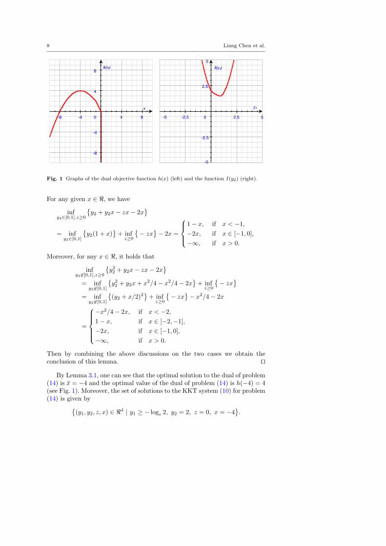
Fig. 1 Graphs of the dual objective function h(x) (left) and the function I(y2) (right).

For any given x ∈ <, we have

infy2∈[0,1],z≥0

{y2 + y2x− zx− 2x

}= infy2∈[0,1]

{y2(1 + x)

}+ infz≥0

{− zx

}− 2x =

1− x, if x < −1,

−2x, if x ∈ [−1, 0],

−∞, if x > 0.

Moreover, for any x ∈ <, it holds that

infy2 6∈[0,1],z≥0

{y22 + y2x− zx− 2x

}= infy2 6∈[0,1]

{y22 + y2x+ x2/4− x2/4− 2x

}+ infz≥0

{− zx

}= infy2 6∈[0,1]

{(y2 + x/2)2

}+ infz≥0

{− zx

}− x2/4− 2x

=

−x2/4− 2x, if x < −2,

1− x, if x ∈ [−2,−1],

−2x, if x ∈ [−1, 0],

−∞, if x > 0.

Then by combining the above discussions on the two cases we obtain theconclusion of this lemma. ut

By Lemma 3.1, one can see that the optimal solution to the dual of problem(14) is x = −4 and the optimal value of the dual of problem (14) is h(−4) = 4(see Fig. 1). Moreover, the set of solutions to the KKT system (10) for problem(14) is given by{

(y1, y2, z, x) ∈ <4 | y1 ≥ − loge 2, y2 = 2, z = 0, x = −4}.

Convergence of ADMM 9

Next, we consider solving problem (14) by using the ADMM scheme (3). Forconvenience, let σ = 1 and set the initial point (x0, y01 , y

02 , z

0) = (0, 0, 0, 0).Now, one should compute (y11 , y

12) by solving

miny1,y2Lσ(y1, y2, z

0;x0).

Define the function I(·) : < → [−∞,+∞] by

I(y2) : = infy1Lσ(y1, y2, z

0;x0)

= infy1

{max

(e−y1 + y2, y

22

)+ (y2 − 2)2/2

}=

{32y

22 − 2y2 + 2 if y2 6∈ [0, 1],

12y

22 − y2 + 2 if y2 ∈ [0, 1].

By direct calculations we can see that the above infimum is attained at y2 = 1with I(y2) = 1.5 (see Fig. 1). However, we have for any y1 ∈ <,

Lσ(y1, 1, 0; 0) = max(e−y1 + 1, 1) + 0.5 = e−y1 + 1.5 > infy1,y2Lσ(y1, y2, z

0;x0).

This means that although infy1,y2 Lσ(y1, y2, z0;x0) = 1.5 is finite, it cannot be

attained at any (y1, y2) ∈ <2. Then the subproblem for computing (y11 , y12) is

not solvable and hence the ADMM scheme (3) is not well-defined. Note thatfor problem (14), Assumption 1 fails to hold since the direction y = (1, 0)satisfies A∗y = 0 and f0+(y) = 0 but f0+(−y) = +∞.

Remark 3.1 The counterexample constructed here is very simple. Yet, onemay still ask if the objective function f about (y1, y2) in problem (14) can bereplaced by an even simpler quadratic function. Actually, this is not possibleas Assumption 1 holds if f is a quadratic function and the original problem hasa solution. Specifically, suppose that α ∈ < is a given number, Q : Y → Y isa self-adjoint positive semidefinite linear operator and a ∈ Y is a given vectorwhile f takes the following form

f(y) = 12 〈y,Qy〉+ 〈a, y〉+ α, ∀ y ∈ Y.

From [11, Pages 67-68] we know that

f0+(y) =

{〈a, y〉, if Qy = 0,

+∞, if Qy 6= 0.(15)

If problem (1) has a solution, one must have f0+(y) ≥ 0 whenever A∗y = 0.This, together with (15), clearly implies that Assumption 1 holds.

10 Liang Chen et al.

4 Convergence Properties of ADMM

The example presented in the previous section motivates us to reconsider theconvergence of the ADMM scheme (3). In the following, we will revisit theconvergence properties of the ADMM, with a computationally more attractivelarge step-length.

For convenience, we introduce some notations, which will be used through-out this section. We use Σf and Σg to denote the two self-adjoint positivesemidefinite linear operators whose definitions, corresponding to the two func-tions f and g in problem (1), can be drawn from (6). Let (x, y, z) ∈ X×Y×Z bea given vector, whose definition will be specified latter. We denote xe := x− x,ye := y − y and ze := z − z for any (x, y, z) ∈ X × Y × Z. If additionally theADMM scheme (3) generates an infinite sequence {(xk, yk, zk)}, for k ≥ 0 wedenote xke := xk − x, yke := yk − y and zke := zk − z, and define the followingauxiliary notations

uk := −A[xk + (1− τ)σ(A∗yke + B∗zke ) + σB∗(zk−1 − zk)],

vk := −B[xk + (1− τ)σ(A∗yke + B∗zke )],

Ψk := 1τσ‖x

ke‖2 + ‖zke ‖2σBB∗ ,

Φk := Ψk + max(1− τ, 1− τ−1)σ‖A∗yke + B∗zke ‖2

(16)

with the convention z−1 ≡ z0. Based on these notations, we have the followingresult.

Proposition 4.1 Suppose that (x, y, z) ∈ X ×Y×Z is a solution to the KKTsystem (10), and that the ADMM scheme (3) generates an infinite sequence{(xk, yk, zk)} (which is guaranteed to be true if Assumptions 1 and 2 hold, cf.Proposition 2.1). Then, for any k ≥ 1,

uk ∈ ∂f(yk), vk ∈ ∂g(zk), (17)

Φk − Φk+1 ≥ 2‖yk+1e ‖2Σf + min(τ, 1 + τ − τ2)σ‖B∗(zk+1 − zk)‖2

+2‖zk+1e ‖2Σg + min(1, 1− τ + τ−1)σ‖A∗yk+1

e + B∗zk+1e ‖2

(18)and

Ψk − Ψk+1 ≥ 2‖yk+1e ‖2Σf + 2‖zk+1

e ‖2Σg + σ‖A∗yk+1e + B∗zke ‖2

+(1− τ)σ‖A∗yk+1e + B∗zk+1

e ‖2.(19)

Proof For any k ≥ 1, the inclusions in (17) directly follow from the first-order optimality condition of the subproblems in the ADMM scheme (3). Theinequality (18) has been proved in Fazel et al.2 [4, parts (a) and (b) in Theorem

2 In [4] the authors studied a much general ADMM-type scheme where positive semidefi-nite proximal terms were added to the subproblems. The convergence properties studied inthis paper can be extended to that setting with no difficulty, but in order to make this noteas concise as possible we focus on ADMM only.

Convergence of ADMM 11

B.1]. Meanwhile, by using (B.12) in [4, Theorem B.1] and (4) we can get

12τσ (‖xke‖2 − ‖xk+1

e ‖2)− σ2 ‖B

∗(zk+1 − zk)‖2 − σ2 ‖B

∗zk+1e ‖2 + σ

2 ‖B∗zke ‖2

− 2−τ2 σ‖A∗yk+1

e + B∗zk+1e ‖2 + σ〈B∗(zk+1 − zk),A∗yk+1

e + B∗zk+1e 〉

≥ ‖yk+1e ‖2Σf + ‖zk+1

e ‖2Σg ,

which, together with the definition of Ψk in (16), implies (19). This completesthe proof. ut

Now, we are ready to present several convergence properties of the ADMMscheme (3).

Theorem 4.1 Assume that the solution set to the KKT system (10) for prob-lem (1) is nonempty. Suppose that the ADMM scheme (3) generates an infinitesequence {(xk, yk, zk)}, which is guaranteed to be true if Assumptions 1 and 2hold. Then, if τ ∈

(0, (1 +

√5 )/2

), one has the following results:

(a) the sequence {xk} converges to an optimal solution to the dual problem (8),and the primal objective function value sequence {f(yk)+g(zk)} convergesto the optimal value;

(b) the sequences {f(yk)} and {g(zk)} are bounded, and if Assumptions 3 and4 hold, the sequences {yk} and {zk} are also bounded;

(c) any accumulation point of the sequence {(xk, yk, zk)} is a solution to theKKT system (10), and if (x∞, y∞, z∞) is one of its accumulation points,then A∗yk → A∗y∞, Σfy

k → Σfy∞, B∗zk → B∗z∞ and Σgz

k → Σgz∞

as k →∞;

(d) if Σf +AA∗ � 0 and Σg + BB∗ � 0, then each of the subproblems in theADMM scheme (3) has a unique optimal solution and the whole sequence{(xk, yk, zk)} converges to a solution to the KKT system (10).

Proof Let (x, y, z) ∈ X × Y × Z be an arbitrary solution to the KKT system(10) of problem (1). We first establish some basic results and then prove (a)to (d) one by one. In the following, the notations provided at the beginning ofthis section are used.

Note that ‖A∗yke‖ ≤ ‖A∗yke + B∗zke ‖ + ‖B∗zke ‖ for any k ≥ 0. Since τ ∈(0, (1 +

√5)/2), by using (16) and (18) we obtain that the sequences

{‖xk‖}, {‖yk‖σAA∗} and {‖zk‖σBB∗} (20)

are all bounded, and

∞∑k=0

‖yke‖2Σf ,∞∑k=0

‖zke ‖2Σg ,∞∑k=0

‖A∗yke + B∗zke ‖2,∞∑k=0

‖B∗(zk+1 − zk)‖2 < +∞.

(21)This, consequently, implies that {uk} and {vk} are bounded sequences. In thefollowing, we prove (a) to (d) separately.

12 Liang Chen et al.

(a) Since {xk} is a bounded sequence, for any one of its accumulation points,e.g. x∞ ∈ X , it admits a subsequence, say, {xkj}j≥0, such that lim

j→∞xkj = x∞.

By using the definitions of {uk} and {vk} in (16) we obtain that

u∞ := limj→∞

ukj = −Ax∞ and v∞ := limj→∞

vkj = −Bx∞. (22)

From (7) and (17) we know that for any k ≥ 1, yk ∈ ∂f∗(uk) and zk ∈ ∂g∗(vk).Hence, we can get A∗yk ∈ A∗∂f∗(uk) and B∗zk ∈ B∗∂g∗(vk) so that

A∗ykj + B∗zkj ∈ A∗∂f∗(ukj ) + B∗∂g∗(vkj ), ∀ j ≥ 0. (23)

Then, by using (21), (22), (23) and the outer semi-continuity of subdifferentialmappings of closed proper convex functions we know that

c ∈ A∗∂f∗(−Ax∞) + B∗∂g∗(−Bx∞),

which implies that x∞ is a solution to the dual problem (8). Therefore, wecan conclude that any accumulation of {xk} is a solution to the dual problem(8). To finish the proof of part (a), we need to show that {xk} is a convergentsequence. This will be done in the following.

We define the sequence {φk}k≥1 by

φk := σ‖zke ‖2BB∗ + max(1− τ, 1− τ−1)σ‖A∗yke + B∗zke ‖2.

Since τ ∈ (0, (1 +√

5)/2), from (18) in Proposition 4.1 and the fact thatΦk ≥ φk, we know that {φk} is a nonnegative and bounded sequence. Thus,there exists a subsequence of {φk}, say {φkl}, such that lim

l→∞φkl = lim inf

k→∞φk.

Since {xkl} is bounded, it must have a convergent subsequence, say, {xkli },such that x := lim

i→∞xkli exists. Note that (x, y, z) is a solution to the KKT

system (10). Therefore, without loss of generality, we can reset x = x from nowon. By using (18) in Proposition 4.1 we know that the nonnegative sequence{Φk} is monotonically nonincreasing, and

limk→∞

Φk = limi→∞

Φkli = limi→∞

( 1

τσ‖xklie ‖2 + φkli

)= lim inf

k→∞φk. (24)

Since 1τσ‖x

ke‖2 = Φk − φk, we have

lim supk→∞

1

τσ‖xke‖2 = lim sup

k→∞{Φk − φk} ≤ lim sup

k→∞Φk − lim inf

k→∞φk = 0, (25)

which indicates that {xk} is a convergent sequence.Now we study the convergence of the primal objective function values. On

the one hand, since (x, y, z) is a saddle point to the Lagrangian function L(·)defined by (9), we have for any k ≥ 1, L(y, z; x) ≤ L(yk, zk; x). This, togetherwith A∗y + B∗z = c, implies that for any k ≥ 1,

f(y) + g(z)− 〈x,A∗yke + B∗zke 〉 ≤ f(yk) + g(zk). (26)

Convergence of ADMM 13

On the other hand, from (17) and (5) we know that

f(yk) + 〈uk, y − yk〉 ≤ f(y) and g(zk) + 〈vk, z − zk〉 ≤ g(z).

By combining the above two inequalities together and using (16) we can get

f(y) + g(z)− 〈xk,A∗yke + B∗zke 〉 − σ〈B∗(zk−1 − zk),A∗yke 〉−(1− τ)σ‖A∗yke + B∗zke ‖2 ≥ f(yk) + g(zk).

(27)

Since the sequences in (20) are bounded, by using (21) and the fact that anynonnegative summable sequence should converge to zero we know that theleft-hand-sides of both (26) and (27) converge to f(y) + g(z) when k → ∞.Consequently, lim

k→∞{f(yk) + g(zk)} = f(y) + g(z) by the squeeze theorem.

Thus, part (a) is proved.

(b) From (17) we konw that for any k ≥ 1,

f(yk) ≤ f(y)− 〈uk, y − yk〉 = f(y)− 〈uk, y〉+ 〈uk, yk〉. (28)

On the one hand, from the boundedness of {uk} we know that the sequence{−〈uk, y〉} is bounded. On the other hand, from (21) and the boundedness ofthe sequences in (20) we can use

〈uk, yk〉 = −〈xk,A∗yk〉 − (1− τ)σ〈A∗yke + B∗zke ,A∗yk〉

−σ〈B∗(zk−1 − zk),A∗yk〉

to get the boundedness of the sequence {〈uk, yk〉}. Hence, from (28) we knowthe sequence {f(yk)} is bounded from above. From (10) we know

f(yk) ≥ f(y) + 〈−Ax, yk − y〉 = f(y)− 〈x,A∗yke 〉,

which, together with the fact that the sequences in (20) are bounded, impliesthat {f(yk)} is bounded from below. Consequently, {f(yk)} is a boundedsequence. By using similar approach, we can obtain that {g(zk)} is also abounded sequence.

Next, we prove the remaining part of (b) by contradiction. Suppose thatAssumption 3 holds and the sequence {yk} is unbounded. Note that the se-quence {yk/(1 + ‖yk‖)} is always bounded. Thus it must have a subsequence{ykj/(1+‖ykj‖)}j≥0, with {‖ykj‖} being unbounded and non-decreasing, con-verging to a certain point ξ ∈ Y. From the boundedness of the sequences in(20) we know that {A∗yk} is bounded. Then we have

A∗ξ = A∗(

limj→∞

ykj

1 + ‖ykj‖

)= limj→∞

A∗ykj1 + ‖ykj‖

= 0.

By noting that ‖ξ‖ = 1, one has ξ ∈ {y ∈ Y | y 6= 0,A∗y = 0}. On the otherhand, define the sequence {dkj}j≥0 by

dkj :=(ykj/(1 + ‖ykj‖) , f(ykj )/(1 + ‖ykj‖)

).

14 Liang Chen et al.

From the boundedness of the sequence {f(ykj )} and the definition of ξ weknow that limj→∞ dkj = (ξ, 0). Since (ykj , f(ykj )) ∈ epi(f), by [11, Theorem8.2] we know that (ξ, 0) is a recession direction of epi(f). Then from thefact that epi(f0+) = 0+(epi f) we know that f0+(ξ) ≤ 0, which contradictsAssumption 3. The boundedness of {zk} under Assumption 4 can be similarlyproved. Thus, part (b) is proved.

(c) Suppose that (x∞, y∞, z∞) is an accumulation point of {(xk, yk, zk)}.Let {(xkj , ykj , zkj )}j≥0 be a subsequence of {(xk, yk, zk)} which converges to(x∞, y∞, z∞). By taking limits in (17) along kj for j →∞ and using (16) and(21) we can see that

−Ax∞ ∈ ∂f(y∞), −Bx∞ ∈ ∂g(z∞) and A∗y∞ + B∗z∞ = c,

and this implies that (x∞, y∞, z∞) is a solution to the KKT system (10).Now, without lose of generality we reset (x, y, z) = (x∞, y∞, z∞). Then, bypart (a) we know that the sequence {Φk} defined in (16) converges to zero ifτ ∈ (0, (1 +

√5)/2). Thus, we always have

limk→∞

‖yke‖Σf = 0 and limk→∞

‖zke ‖σBB∗+Σg = 0. (29)

As a result, it holds that B∗zk → B∗z∞, Σfyk → Σfy

∞ and Σgzk → Σgz

∞

as k → ∞. Moreover, by using the fact that A∗yk = (A∗yk + B∗zk) − B∗zkand A∗yk + B∗zk → A∗y∞ + B∗z∞ = c as k →∞, we can get A∗yk → A∗y∞as k →∞. This completes the proof of part (c).

(d) If Σf +AA∗ � 0 and Σg +BB∗ � 0, then the subproblems in the ADMMscheme (3) are strongly convex, and hence each of them has a unique optimalsolution. Then, by part (c) we know that {yk} and {zk} are convergent. Notethat the sequence {xk} is convergent by part (a). Therefore, by part (c) weknow that {(xk, yk, zk)} converges to a solution to the KKT system (10).Hence, part (d) is proved and this completes the proof of the theorem.

Before concluding this note, we make the following remarks on the conver-gence results presented in Theorem 4.1.

Remark 4.1 The corresponding results in part (a) of Theorem 4.1 for theADMM scheme (3) with τ = 1 have been stated in Boyd et al. [1]. How-ever, as indicated by the counterexample constructed in Section 3, the proofsin [1] need to be revised with proper additional assumptions. Actually, noproof on the convergence of {xk} has been given in [1] at all. Nevertheless,one may view the results in part (a) as extensions of those in Boyd et al. [1]for the ADMM scheme (3) with τ = 1 to a computationally more attractiveADMM scheme (3) with a rigorous proof.

Remark 4.2 Note that, numerically, the boundedness of the sequences gener-ated by a certain algorithm is a desirable property and Assumptions 3 and 4can fulfill this purpose. Assumption 3 is rather mild in the sense that it holdsautomatically for many practical problems where f has bounded level sets. Ofcourse, the same comment can also be applied to Assumption 4.

Convergence of ADMM 15

Remark 4.3 All the results of Theorem 4.1 are also valid if the step-length τand the sequence generated by the ADMM scheme (3) satisfy the conditionthat

τ ≥ (1 +√

5)/2 but

∞∑k=1

‖xk+1 − xk‖2 < +∞. (30)

To prove this argument, one can first use xk+1 − xk = τσ(A∗yk+1e + B∗zk+1

e )to get

∑∞k=0 ‖A∗yke + B∗zke ‖2 < +∞. Then, by using (19) and the fact that

‖A∗yke‖ ≤ ‖A∗yke+B∗zke ‖+‖B∗zke ‖ we know the sequences in (20) are bounded.Note that ‖B∗(zk+1 − zk)‖2 ≤ 2‖A∗yk+1

e + B∗zk+1e ‖2 + 2‖A∗yk+1

e + B∗zke ‖2.This, together with (19), implies that (21) holds. The remaining procedure issimilar to that for Theorem 4.1 except the following two key steps.

The first one is to show that {xk} is convergent. To do this, we define thenonnegative sequence {ψk} by ψk := σ‖zke ‖2BB∗ . By using (19), (21), Lemma2.1 and fact that 1 − τ < 0 one can show that the sequence {Ψk} is conver-gent. Hence, the sequence {ψk} is nonnegative and bounded. Then, by similardiscussions for getting (24) and (25) with φk and Φk being replaced by ψk andΨk, one can get lim

k→∞Ψk = lim inf

k→∞ψk. and Hence, {xk} is convergent.

The second one is to show that (29) still holds for this case. This can bedone by verifying that the sequence {Ψk} defined in (16) converges to zero ifτ ≥ (1 +

√5)/2 but

∑∞k=0 ‖xk+1 − xk‖2 < +∞.

The condition (30) simplifies the condition proposed by Sun et al. [13, The-orem 2.2], in which one need

∑∞k=1{‖B∗(zk+1−zk)‖2 +σ‖xk+1−xk‖2} < +∞

if τ ≥ (1 +√

5)/2. This was used for the purpose of achieving better numer-ical performance. The advantage of taking the step-length τ ≥ (1 +

√5)/2

has been observed in [2,10,13] for solving high-dimensional linear and convexquadratic semidefinite programming problems. In numerical computations, onecan start with a larger τ , e.g. τ = 1.95, and reset it as τ := max(γτ, 1.618)for some γ ∈ (0, 1), e.g. γ = 0.95, if at the k-th iteration one observes that‖xk+1 − xk‖2 > c0/k

1.2, where c0 is a given positive constant. Since τ can bereset at most a finite number of times, our convergence analysis is valid forsuch a strategy. One may refer to [13, Remark 2.3] for more discussions onthis computational issue.

5 Conclusions

In this note, we have constructed a simple example possessing several niceproperties to illustrate that the convergence theorem of the ADMM scheme(3) with the unit step-length stated in Boyd et al. [1] can be false if no priorcondition that guarantees the existence of solutions to all the subproblemsinvolved is made. In order to correct this mistake we have presented fairlymild conditions under which all the subproblems are solvable by using stan-dard knowledge in convex analysis. Based on these conditions, we have furtherestablished some satisfactory convergence properties of the ADMM with a

16 Liang Chen et al.

computationally more attractive large step-length that can exceed the goldenratio of (1 +

√5)/2. In conclusion, this note has (i) clarified some confusions

on the convergence results of the popular ADMM; (ii) opened the potential fordesigning computationally more efficient ADMM based solvers in the future.

Acknowledgements The authors would like to thank the two anonymous referees for theircareful reading of this paper and their comments to improve the quality of this paper. Theauthors also would like to thank the corresponding editor for providing insightful suggestions.

References

1. Boyd, S., Parikh, N., Chu, E., Peleato, B. and Eckstein, J.: Distributed optimization andstatistical learning via the alternating direction method of multipliers. Found. TrendsMach. Learn. 3(1),1–122 (2011)

2. Chen, L., Sun, D.F. and Toh, K.-C.: An effcient inexact symmetric Gauss-Seidel basedmajorized ADMM for high-dimensional convex composite conic programming. Math.Program. doi: 10.1007/s10107-016-1007-5 (2016)

3. Eckstein, J. and Yao, W.: Understanding the convergence of the alternating directionmethod of multipliers: theoretical and computational perspectives. Pac. J. Optim. 11(4),619–644 (2015)

4. Fazel, M., Pong, T.K., Sun, D.F. and Tseng, P.: Hankel matrix rank minimization withapplications to system identification and realization. SIAM J. Matrix Anal. Appl. 34(3),946–977 (2013)

5. Fortin, M., Glowinski, R.: Augmented Lagrangian Methods. Applications to the Numer-ical Solution of Boundary Value Problems. Studies in Mathematics and its Applications,15. Translated from the French by B. Hunt and D. C. Spicer. Elsevier Science publishersB.V. (1983)

6. Gabay, D., Mercier, B.: A dual algorithm for the solution of nonlinear variational prob-lems via finite element approximation. Comput. Math. Appl. 2(1), 17–40 (1976)

7. Glowinski, R.: Lectures on numerical methods for non-linear variational problems. Pub-lished for the Tata Institute of Fundamental Research, Bombay [by] Springer-Verlag(1980)

8. Glowinski, R.: On alternating direction methods of multipliers: A historical perspective.In Fitzgibbon, W., Kuznetsov, Y.A., Neittaanmaki, P. and Pironneau, O. (eds.) Mod-eling, Simulation and Optimization for Science and Technology, pp. 59–82. Springer,Netherlands (2014)

9. Glowinski, R and Marroco, A.: Sur l’approximation, par elements finis d’ordre un,et la resolution, par penalisation-dualite d’une classe de problemes de Dirichlet nonlineaires. Revue francaise d’atomatique, Informatique Recherche Operationelle. Anal-yse Numerique 9(2), 41–76 (1975)

10. Li, X.D., Sun, D.F. and Toh, K.-C.: A Schur complement based semi-proximal ADMMfor convex quadratic conic programming and extensions. Math. Program. 155, 333-373(2016)

11. Rockafellar, R.T.: Convex Analysis. Princeton University Press (1970)12. Rockafellar, R.T. and Wets, R. J-B: Variational Analysis. Springer, Verlag Berlin Hei-

delberg (2009)13. Sun, D.F., Toh, K.-C. and Yang, L.Q.: A convergent 3-block semi-proximal alternating

direction method of multipliers for conic programming with 4-type constraints. SIAMJ. Optim. 25, 882–915 (2015)