A NOVEL HYBRID METHOD FOR THE SEGMENTATION OF …airccse.org/journal/jcsit/5313ijcsit04.pdf ·...

International Journal of Computer Science & Information Technology (IJCSIT) Vol 5, No 3, June 2013

DOI : 10.5121/ijcsit.2013.5304 45

A NOVEL HYBRID METHOD FOR THE

SEGMENTATION OF THE CORONARY ARTERY TREE IN 2D ANGIOGRAMS

Daniel S.D. Lara1, Alexandre W.C. Faria2, Arnaldo de A. Araújo1, and D. Menotti3

1Computer Science Department, Univ. Fed. de Minas Gerais, Belo Horizonte, Brazil {daniels,arnaldo}@dcc.ufmg.br

2Graduate Program in Electrical Engineering, UFMG, Belo Horizonte, Brazil [email protected]

3Computing Department, Universidade Federal de Ouro Preto, Ouro Preto, Brazil [email protected]

ABSTRACT Nowadays, medical diagnostics using images have considerable importance in many areas of medicine. Specifically, diagnoses of cardiac arteries can be performed by means of digital images. Usually, this diagnostic is aided by computational tools. Generally, automated tools designed to aid in coronary heart diseases diagnosis require the coronary artery tree segmentation. This work presents a method for a semi-automatic segmentation of the coronary artery tree in 2D angiograms. In other to achieve that, a hybrid algorithm based on region growing and differential geometry is proposed. For the validation of our proposal, some objective and quantitative metrics are defined allowing us to compare our method with another one proposed in the literature. From the experiments, we observe that, in average, the proposed method here identifies about 90% of the coronary artery tree while the method proposed by Schrijver & Slump (2002) identifies about 80%. KEYWORDS Image Segmentation, Coronary Artery Tree, Angiography.

1. INTRODUCTION Blood vessels detection is an important step in many medical application tasks, such as automatic detection of vessel malformations, quantitative coronary analysis (QCA), vessel centerline extractions, etc. Blood vessel segmentation algorithms are the key components of automated radiological diagnostic systems [1]. A wide variety of automatic blood vessel segmentation methods has been proposed in the last two decades. These methods used approaches that varied from Pattern Recognition techniques [2,3], Model-based Approaches [4, 5,6 ], Texture Analysis [7], Tracking-Based Approaches [8,9], Artificial Intelligence Approaches [10] until Neural Network-based approaches [11]. Even with all these efforts, only few of these methods achieved enough results to be applied in a system allowing the user to give a minimum input. Once these input parameters are introduced, the user does not need to work for obtaining the segmentation given similar quality images. However, the nature of X-Ray angiograms leads to a possible low or high contrast images depending on the patient weight. This work presents a novel hybrid region growing method with a differential geometry vessel detector for the segmentation and identification of the cardiac coronary tree in 2D angiograms. That is, it incorporates advantages from other works, for example, the simplicity of the work proposed by O’Brien & Ezquerra (1994) [12] and robustness of the work proposed by Schrijver (2002) [13]. Observe that a preliminary version of this work appears in [14], and hybrid region


46

growing methods has been recently published in this subject [15, 16]. Figure 1 shows an overview of the proposed method.

Figure 1. Flowchart of the proposed method

This paper is organized as follows. Section 2 describes the segmentation method, in which Section 2.1 gives details regarding the angiography contrast enhancement step, Section 2.2 explains in the region growing step, Sections 2.3 and 2.4 explain the vessel resemblance function and the seed selection process, Section 2.5 illustrates the connected component analysis, and Section 2.5 presents the algorithm for the whole segmentation process. At the end of this section, in Section 2.7, a brief complexity analysis of our algorithm is shown. Analysis of results of our method is presented in Section 5, which uses the metrics defined in Section 4 and the database described in Section 3. And finally, conclusions and future works are pointed out in Section 6.

2. METHOD A common problem in methods based in only region growing is their difficulty to continue growing the segmented area if any artefact or vessel blockage (e.g., stenosis) drives the region to a minimum area to be segmented (discontinuities). Aiming to avoid these non desired characteristics, this proposal starts with an automatic contrast enhancement step based in CLAHE (Contrast Limited Adaptive Histogram Equalization) followed by a region growing and finalizing by a differential geometry vessel detector. The next subsections will explain each step in details. 2.1. Contrast limited adaptive histogram equalization (CLAHE) In this work, CLAHE is used as a first step for image enhancement. Figure 2 illustrates the enhancement produced for an angiography with poor levels of contrast using this algorithm.


47

Figure 2: CLAHE example

2.2. Region growing In order to propose an automatic segmentation method, a local search could be a good starting option for coronary identification. Furthermore, more sophisticated solutions (which can include global searches) can be incorporated to the initial local search to refine the results. The region growing step proposed here starts with a first vessel point given by a user mouse click. O’Brien & Ezquerra (1994) [12] formalized part of this idea as the following: Once an initial point, ),(0 yxS which lies somewhere on the vessel structure is available, a search will be performed. Thus, the following assumptions are used: 1. The area which is part of the vessels is required to be “slightly darker” than the background; 2. For some sample area in the image, such as a circle window, if the area is large enough, the

ratio of vessel area to background area, say av/ab, will be less than some constant C and greater than other constant D for each image;

3. The vessel segments are “elongated” structures; 4. The width of a healthy (non-stenotic) blood vessel changes ”slow”; 5. The pixel values change “slowly” along with the length of the connected vessels except

where some object may intersect or occlude the blood vessel (e.g., overlapping bifurcations). In this way, starting with an initial seed S0(x,y) , the method defines a circle centred in S0 with radius r0. Niblack thresholding equation [17, pages 115-116] is used to identify two classes (vessel and background) of pixels in the circle. Then let t be the Niblack threshold for a circle c. The vessel diameter d0 at the circle extremity can be identified by calculating the greatest axis of the ellipse that better adjust to the pixels located at the border of the segmented circle. This ellipse can be found from the normalized second central moments of the connected component determined by the segmented circle portion over its perimeter [18]. Figure 3 presents an example of the diameter determination of the blood vessel at the extremity of the circle c. The greatest axis of this ellipse, in yellow, represents the artery diameter. The green point illustrates a new region growing seed. Once d0 is found, its mean point becomes a new seed S1. A new circle with radius d0 centred in S1 is traced and the segmentation process starts again. This recursive step is then repeated until the diameter dn reaches a minimum value m. Furthermore, in order to avoid divergence cases, dn is limited to a maximum value M. Figure 4 shows the above idea graphically.


48

Figure 3: Exemple of coronary diameter estimation

Figure 4: Region growing algorithm

2.3. Vessel resemblance function The step followed by the region growing is the Vessel Resemblance Function computation. This function proposed by [19] assigns vessel resemblance values for each pixel of the angiography. Let the angiography g(u,v) be seen as a three-dimensional surface as: G={(u,v,z)|z=g(u,v)}, (1) where u and v extends over the support of g(u,v). Then, for all grid point x=(u,v), the surface curvature is described by the Hessian matrix H(x):

)()()()(

)(xgxgxgxg

xHvvvu

uvuu , (2)

where guu(x), guv(x)=gvu(x), and gvv(x) are the second-order spatial derivatives of g(x). These derivatives can be calculated by a convolution of a second order spatial derivatives of a Gaussian filter at a scale σ with g(x) [19],[20]:

gab(x;σ)=σ2hab(x;σ)*g(x). (3) From an analysis of the eigenvalues and eigenvectors of the Hessian matrix, it is noticeable that the Hessian matrix strongest eigenvalue and its corresponding eigenvector in a point (u,v) give the 3D-surface strongest curvature and its direction. The eigenvector corresponding to the weaker eigenvalue represents the surface direction perpendicular to the strongest curvature. As the Hessian matrix is a function of scale σ then the eigenvalues are also. Furthermore λi could be written as λi(x;σ). However, supposing we are working with only one scale, and for simplicity, it will be abbreviated by λi and its corresponding eigenvector by vi. For the subsequent analysis, it is supposed the eigenvalues are ordered according to: |λ1|≥|λ2|. (4)

In this way, assuming an angiography point x=(u,v) being part of a vessel, the eigenvector v1 is perpendicular to the vessel in x. It happens because the vessels are considered to be a darker region against a brighter background. It means the strongest Hessian eigenvalue is positive in x and the strongest surface curvature is perpendicular to the vessel in x. Furthermore, v2 will be parallel to the vessel in x. Also, the assumption 3 proposed by O’Brien & Ezquerra (1994) [12]


49

allows us to conclude that the weaker Hessian eigenvalue should be small in x. In other words, the surface G has a little curvature on the vessel direction. The following summarizes these characteristics for the vessel point x=(u,v): 01 and 02 (5)

Based on all these considerations, the following vessel resemblance function V(x;σ), is defined ([20]):

V(x;σ)=

0 if λ1<0 ;

exp

R

2B

2β21

1-exp

-S2

2β22

otherwise , (6)

where RB is a measure of how |λ1| is bigger than |λ2|, i.e.,

RB= |λ2||λ1|, (7)

and S is a measure of the strength of the overall curvature:

S= λ21+λ

22. (8)

The parameters β1>0 and β2>0 are scaling factors influencing the sensitivity to RB and S respectively.

(a) (b)

Figure 5: Vessel resemblance function results: (a) Image processed by Contrast Limited Adaptive Histogram Equalization; (b) Respective result.

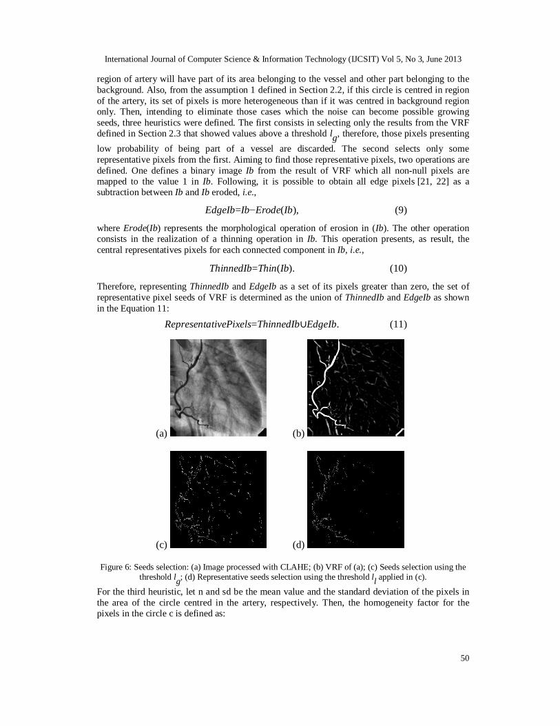
Images in Figure 5 show some angiographies processed by applying the vessel resemblance function. Next subsection explains how to use these results to obtain region growing seeds automatically. 2.4. Seeds selection The Vessel Resemblance Function returns a value for each pixel in the angiography. In the images of Figure 5, most part of the non-null pixels belongs to the vessels. All those pixels greater than zero are new possible growing seeds. However, some noise or image artifacts can contribute for a small part of background being misunderstood as vessels. These non desired results need to be eliminated to minimize the false positive effect on the segmented object. In this way, from the assumption 2 defined in Section 2.2, it is expected that the circle centred in any


50

region of artery will have part of its area belonging to the vessel and other part belonging to the background. Also, from the assumption 1 defined in Section 2.2, if this circle is centred in region of the artery, its set of pixels is more heterogeneous than if it was centred in background region only. Then, intending to eliminate those cases which the noise can become possible growing seeds, three heuristics were defined. The first consists in selecting only the results from the VRF defined in Section 2.3 that showed values above a threshold lg, therefore, those pixels presenting low probability of being part of a vessel are discarded. The second selects only some representative pixels from the first. Aiming to find those representative pixels, two operations are defined. One defines a binary image Ib from the result of VRF which all non-null pixels are mapped to the value 1 in Ib. Following, it is possible to obtain all edge pixels [21, 22] as a subtraction between Ib and Ib eroded, i.e.,

EdgeIb=Ib−Erode(Ib), (9)

where Erode(Ib) represents the morphological operation of erosion in (Ib). The other operation consists in the realization of a thinning operation in Ib. This operation presents, as result, the central representatives pixels for each connected component in Ib, i.e.,

ThinnedIb=Thin(Ib). (10)

Therefore, representing ThinnedIb and EdgeIb as a set of its pixels greater than zero, the set of representative pixel seeds of VRF is determined as the union of ThinnedIb and EdgeIb as shown in the Equation 11:

RepresentativePixels=ThinnedIb∪EdgeIb. (11)

(a) (b)

(c) (d)

Figure 6: Seeds selection: (a) Image processed with CLAHE; (b) VRF of (a); (c) Seeds selection using the threshold lg; (d) Representative seeds selection using the threshold ll applied in (c).

For the third heuristic, let n and sd be the mean value and the standard deviation of the pixels in the area of the circle centred in the artery, respectively. Then, the homogeneity factor for the pixels in the circle c is defined as:


51

HomoFact= n−sd

n . (12) Note that when HomoFact gets close to the value 1, it means the circle area is more homogeneous. Thus, a filtering, realized for every representative pixel originated in the second heuristic, is used to determine if a seed pixel belongs to a background or coronary area. Figure 6 presents the seeds selection result for a right coronary angiography.

This process gives, as result, an image containing seed pixels on the vessel regions. These seed pixels are used as input for a new region growing step as described in the Section 2.2.

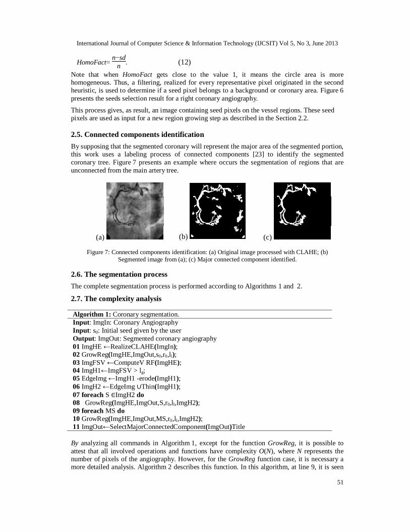
2.5. Connected components identification By supposing that the segmented coronary will represent the major area of the segmented portion, this work uses a labeling process of connected components [23] to identify the segmented coronary tree. Figure 7 presents an example where occurs the segmentation of regions that are unconnected from the main artery tree.

(a) (b) (c)

Figure 7: Connected components identification: (a) Original image processed with CLAHE; (b) Segmented image from (a); (c) Major connected component identified.

2.6. The segmentation process The complete segmentation process is performed according to Algorithms 1 and 2.

2.7. The complexity analysis Algorithm 1: Coronary segmentation. Input: ImgIn: Coronary Angiography Input: s0: Initial seed given by the user Output: ImgOut: Segmented coronary angiography 01 ImgHE ←RealizeCLAHE(ImgIn); 02 GrowReg(ImgHE,ImgOut,s0,r0,ll); 03 ImgFSV ←ComputeV RF(ImgHE); 04 ImgH1←ImgFSV > lg; 05 EdgeImg ←ImgH1 -erode(ImgH1); 06 ImgH2 ←EdgeImg ∪Thin(ImgH1); 07 foreach S ∈ImgH2 do 08 GrowReg(ImgHE,ImgOut,S,r0,ll,ImgH2); 09 foreach MS do 10 GrowReg(ImgHE,ImgOut,MS,r0,ll,ImgH2); 11 ImgOut←SelectMajorConnectedComponent(ImgOut)Title By analyzing all commands in Algorithm 1, except for the function GrowReg, it is possible to attest that all involved operations and functions have complexity O(N), where N represents the number of pixels of the angiography. However, for the GrowReg function case, it is necessary a more detailed analysis. Algorithm 2 describes this function. In this algorithm, at line 9, it is seen


52

that all processed circle c is extracted from the generated seeds set. For this reason, it is possible to say that, in the worst case, the GrowReg function will process all pixels in the image. Therefore, it is possible to conclude that Algorithm 1 also has time complexity of O(N), where N represents the number of pixels of the angiography. Note that the third heuristic defined in Section 2.4 is implemented in the function GrowReg. Algorithm 2: GrowReg function. Algorithm 2: GrowReg function. Input: ImgHE: Coronary angiography processed by CLAHE Input: s0: Initial segmentation point Input: r0: Initial radius for the propagation circle co Input: ll: Local segmentation threshold Output: ImgH2: Selected seeds in VRF Output: ImgOut: Segmented coronary angiography with many connected components 01 if llcnccn )(/))()(( then 02 return; 03 T(c) ←n(c) + 0.2 ×σ(c); 04 foreach p ∈c do 05 if ImgHE(c(p)) ≤T(c) then 06 ImgOut(c(p)) ←0; 07 else 08 ImgOut(c(p)) ←1; 09 ImgH2 ←ImgH2 -Segmented(c); 10 r ←ComputeDiameter(c); 11 NewSeeds ←IdentifyNewSeeds(ImgOut(c)); 12 foreach Sn ∈NewSeeds do 13 GrowReg(ImgHE,ImgOut,Sn,r,ll,ImgH2)

3. THE DATABASE Before presenting the metrics used to evaluate the results obtained by our proposed method, we describe the database of angiographies used and also the ground truth images.

3.1. The database In order to evaluate the proposed method, 52 Left Coronary Artery (LCA) angiographies, 46 Right Coronary Artery (RCA) angiographies and 2 bypass operation angiographies were sampled. Usually, the RCA has fewer ramifications than the LCA, for this reason, a base containing a greater number of LCA will not make the segmentation process easier.

Furthermore, a study about the base images was performed to identify quantitative information about the first and second order coronaries. It was verified that the first order coronaries have a mean radius value of 12 pixels whilst the second order coronaries have a mean radius value of 6 pixels. All images are 1024×1024 pixels, 8 bits gray-scale, and they were recorded using a SISMED Digitstar 600N system.

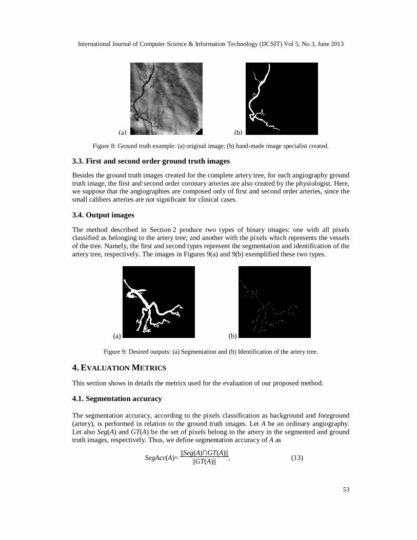
3.2. Ground truth images The ground truth images, or reference images, used in this work represent the ideal angiography segmentation. For each angiography of the database, a manual segmentation of the artery tree is created by a physiologist (specialist in angiography). This image represents the result segmentation that our method should achieve. The image in Figure 8(b) shows a ground truth image of the angiography shown in Figure 8(b).


53

(a) (b)

Figure 8: Ground truth example: (a) original image; (b) hand-made image specialist created. 3.3. First and second order ground truth images Besides the ground truth images created for the complete artery tree, for each angiography ground truth image, the first and second order coronary arteries are also created by the physiologist. Here, we suppose that the angiographies are composed only of first and second order arteries, since the small calibers arteries are not significant for clinical cases. 3.4. Output images The method described in Section 2 produce two types of binary images: one with all pixels classified as belonging to the artery tree; and another with the pixels which represents the vessels of the tree. Namely, the first and second types represent the segmentation and identification of the artery tree, respectively. The images in Figures 9(a) and 9(b) exemplified these two types.

(a) (b)

Figure 9: Desired outputs: (a) Segmentation and (b) Identification of the artery tree.

4. EVALUATION METRICS This section shows in details the metrics used for the evaluation of our proposed method. 4.1. Segmentation accuracy The segmentation accuracy, according to the pixels classification as background and foreground (artery), is performed in relation to the ground truth images. Let A be an ordinary angiography. Let also Seg(A) and GT(A) be the set of pixels belong to the artery in the segmented and ground truth images, respectively. Thus, we define segmentation accuracy of A as

SegAcc(A)= ||Seg(A)∩GT(A)||

||GT(A)|| , (13)


54

where ||X|| stands for the cardinality of X. Despite the fact that this metric determine how accurate is the segmentation in relation to the arteries, it is important to define the segmentation accuracy in relation to the entire angiography, i.e.,

SegAccG(A)= ||Seg(A)∩GT(A)||

||A|| . (14)

Besides evaluating how the segmentation is right, it is also important to measure how the segmentation is wrong. Then, we can have both false-positive (FP) and false-negative (FN) pixels. That is, the former are composed of those pixels belong to the background, but they are classified as foreground (artery), and the latter are composed of those pixels belong to the foreground, but they are classified as background. Then, we can define

SegAccFP= ||Seg(A)∩ GT(A) ||

|| GT(A) ||, (15)

and

SegAccFN= || Seg(A) ∩GT(A)||

|| GT(A) ||, (16)

where X denotes the complementary set of pixels of X, being the universe of X the domain of the image. And, in a similar way to Equation 14, we can define

SegAccGFP= ||Seg(A)∩ GT(A) ||

||A|| , (17)

and

SegAccGFN= || Seg(A) ∩GT(A)||

||A|| . (18)

Figure 10 illustrates these definitions. Note that all metrics defined in this section can be computed for both the first and second order arteries. And GT(A) is equal to

GT(A1)∪GT(A2) , where GT(A1) and GT(A2) stand for the first and second order arteries

ground truth images of A, respectively.

(a) (b) (c) (d)

Figure 10: Segmentation accuracy: (a) Image to be segmented; (b) Ground truth image of (a); (c) Segmentation resulting from (a); Image with highlight errors, where the pixels in red, blue, and green

represent the false-positives, false-negatives, and true-positives, respectively.

In order to make easier the analysis of the results, in Section 5, the metrics defined here in relation to the complete angiography, are presented in confusion matrices.


55

4.2. Identification accuracy

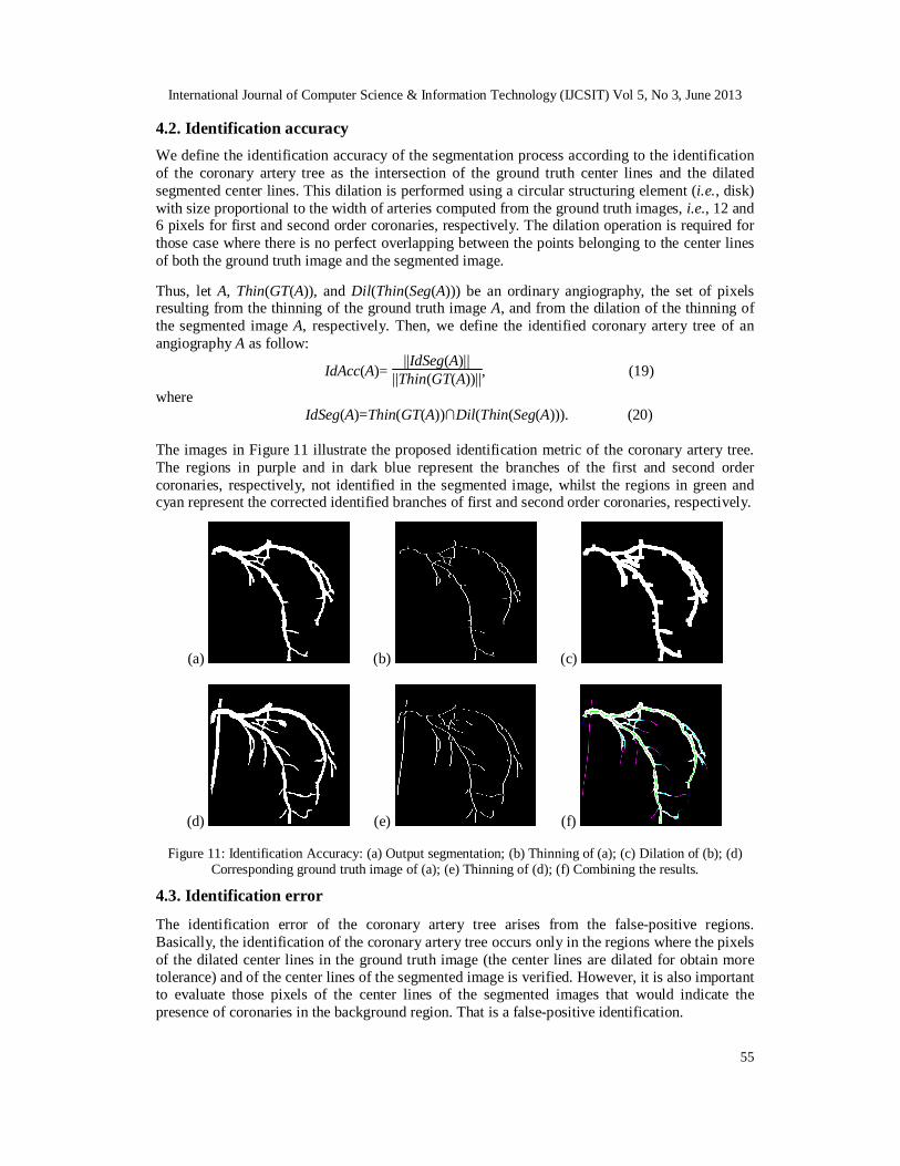
We define the identification accuracy of the segmentation process according to the identification of the coronary artery tree as the intersection of the ground truth center lines and the dilated segmented center lines. This dilation is performed using a circular structuring element (i.e., disk) with size proportional to the width of arteries computed from the ground truth images, i.e., 12 and 6 pixels for first and second order coronaries, respectively. The dilation operation is required for those case where there is no perfect overlapping between the points belonging to the center lines of both the ground truth image and the segmented image. Thus, let A, Thin(GT(A)), and Dil(Thin(Seg(A))) be an ordinary angiography, the set of pixels resulting from the thinning of the ground truth image A, and from the dilation of the thinning of the segmented image A, respectively. Then, we define the identified coronary artery tree of an angiography A as follow:

IdAcc(A)= ||IdSeg(A)||

||Thin(GT(A))||, (19)

where IdSeg(A)=Thin(GT(A))∩Dil(Thin(Seg(A))). (20) The images in Figure 11 illustrate the proposed identification metric of the coronary artery tree. The regions in purple and in dark blue represent the branches of the first and second order coronaries, respectively, not identified in the segmented image, whilst the regions in green and cyan represent the corrected identified branches of first and second order coronaries, respectively.

(a) (b) (c)

(d) (e) (f)

Figure 11: Identification Accuracy: (a) Output segmentation; (b) Thinning of (a); (c) Dilation of (b); (d) Corresponding ground truth image of (a); (e) Thinning of (d); (f) Combining the results.

4.3. Identification error The identification error of the coronary artery tree arises from the false-positive regions. Basically, the identification of the coronary artery tree occurs only in the regions where the pixels of the dilated center lines in the ground truth image (the center lines are dilated for obtain more tolerance) and of the center lines of the segmented image is verified. However, it is also important to evaluate those pixels of the center lines of the segmented images that would indicate the presence of coronaries in the background region. That is a false-positive identification.


56

Thus, let A, Thin(Seg(A)), and Dil(Thin(GT(A))) be an angiography, the set of pixels resulting from the thinning of the segmented image A, and from the dilation of the thinning of the ground truth image of A, respectively. Then, we define the identification error as:

IdError= ||Thin(Seg(A))∩ Dil(Thin(GT(A))) ||

||Thin(GT(A))|| , (21)

where X stands for the complementary set of pixels of X regarding its universe, i.e., the angiography X. The images in Figure 12 illustrate the identification error metric. In the identification, the result errors are highlighted in green.

(a) (b) (c)

(d) (e) (f)

Figure 12: Identification error of the coronary artery tree: (a) Ground truth image; (b) Thinning of (a); (c) Dilation of (b); (d) Segmented image; (e) Thinning of (d); (f) Identification result where the errors are

highlighted in green. It is worth noting that this metric can yield figures greater than 100%. This happens in the case where the thinning of Seg(A) produce a lot of branches. For example, when we have a false-positive high rate, such that the cardinality of Thin(Seg(A)) is quite greater than the cardinality of Thin(GT(A)) (at least twice), IdError produces as results a value over 100%.

5. EXPERIMENTAL RESULTS This section presents the experimental results obtained with the implementation of the proposed method in Section 2. Moreover, all results that could be compared with those shown by Schrijver (2002) [13] were presented and analyzed. The reported experiments were processed in a Intel Core 2 Duo 6600 2.4 GHz Computer, with 2GBytes of memory and Microsoft Windows XP as Operational System. Also, the implementation was realized using MatLab. The mean processing time for each image was about 20 seconds.

5.1. Control points evaluation This section presents a behaviour analysis of the results presented by the proposed method when its parameter varies. Basically, there exist only three parameters for the proposed algorithm. The first one is the parameter to determine the initial propagation radius r0 for each growing seed. The


57

last two, lg and ll, are global and local thresholds, respectively, that were presented in Section 2.4. Any other parameter that may be used in any other step, such as, for example, those used in the CLAHE processing or VRF determination, are static values and were chosen in accordance with the best values suggested in literature. Aiming to find a balance of values, these three parameters were changed one to one for a 10 images base, chosen randomly, and the results for segmentation exactness of first order and second order coronaries, precision of centerlines, precision of edges, mean processing time and identification error for the coronary tree were registered. Tables 1, 4, and 9 were created to compare these values. For each table, two parameters were static and the third varied. In this way, it was possible to verify the best result for each set of values. The terms Seg. P./S., F.P., E.I.P./S., P.L.M., P.B., T.M. e Er.Id. are abbreviations for First/Second order segmentation, false-positive percentage, exactness of the identification of First/Second order coronaries, precision of centerlines, precision of edges, mean time processing and error of identification of the coronary tree, respectively. For the first table creation, it was decided to vary r0. Therefore, it was necessary to choose static values for lg and ll. Empirically, it was chosen lg=0.2 and ll=0.85.

Table 1: Evaluation of the parameters for the proposed method varying r0.

r0 lg ll Seg. P./S. F.P. E.I.P./S. P.L.M. P.B. T.M. Er.Id. pix. abs. abs. % % % pixels pixels seg. % 5 0.2 0.85 79.32/64.82 1.14 90.20/73.38 3.34 3.70 29.6 16.03 10 0.2 0.85 83.17/74.03 1.72 94.13/84.37 3.24 3.62 26.9 25.50 15 0.2 0.85 85.42/77.52 2.46 94.80/82.66 3.42 3.51 19.7 36.58 20 0.2 0.85 88.57/80.31 3.39 97.96/84.00 3.67 3.76 15.4 53.37 25 0.2 0.85 90.29/85.38 4.10 98.33/86.50 3.65 3.90 13.4 65.03 30 0.2 0.85 90.67/86.40 4.73 98.14/86.85 4.72 4.31 13.6 77.87 35 0.2 0.85 92.07/85.71 6.05 97.77/86.49 4.06 4.73 14.1 93.76 40 0.2 0.85 93.00/85.58 7.19 97.83/83.83 4.05 4.70 14.6 107.41 45 0.2 0.85 93.47/88.17 8.01 97.63/85.20 4.27 5.13 15.6 117.65 50 0.2 0.85 94.02/88.92 8.49 95.55/84.44 4.39 6.06 16.9 123.17

5.1.1. Evaluating r0

Table 1 shows the results obtained varying r0 from 5 to 50 in steps of 5. As expected, from the results shown in Table 1, it was possible to note that an increase in r0 values induces another increase on the percentage of the segmented coronary tree. However, it also increases the percentage of false-positives, the error of the centerlines, the error of the edges and the error of the coronary tree identification. The confusion matrix of Table 2 presents the result of this analysis for the case where it presented the best segmentation percentage i.e., r0=50 pixels. Table 3 shows the percentages for the segmentation results for r0=50.


58

Table 2: Confusion matriz of the segmentation process for r0=50, lg=0.2 and ll=0.85.

Exp. \Obs. First Order Second Order

Background

First Order 4.9±1.0 0.3±0.3

Second Order 1.8±1.0 0.2±0.3

Background 8.5±3.4 84.3±4.1

Table 3: Percentages of the segmentation process for r0=50, lg=0.2 and ll=0.85.

Exp.\Obs. First Order Second Order

Background

First Order 94.0±3.7 6.0±3.7

Second Order 88.9±9.8 11.1±9.8

Background 9.1±3.8 90.8±9.8

By analyzing Table 2, it is visible that, in a mean value, 8.49% of the image pixels belonging to the background were identified as belonging to the coronary tree, whilst the real number of pixels belonging to the coronary tree sums 7.25% (4.91% + 1.78% 0.33% + 0.23%) of the image pixels. It means that the number of false-positives surpassed the real number of pixels belonging to the coronaries. In other words, it identified more background as being coronaries than the real ground truth coronaries.

Figure 13: Segmentation result of the coronary artery tree for (a) r0=50 and (b) r0=10

Taking into account the observed above, aiming to maximize the segmentation rates of the coronary tree and, at the same time, to minimize the segmented false-positive rates, as well, the error of coronary identification, a parameter choice for r0 could be r0=10 pixels. The image of Figure 13(b) shows the segmentation result using r0=10 for the same input image used to obtain the output image in Figure 13(a). In terms of false-positives, the result presented in Figure 13(b) shows an improvement when compared with the result shown in Figure 13(a). However, it still do have false-positives. Furthermore, false-negatives appeared identified in blue color.

Table 4: Parameter evaluation of the proposed method varying lg.


59

5.1.2. Evaluating ll Intending to study the behavior of the other parameters, the next analysis progresses establishing r0=10, ll=0.85 and varying lg in a range between 0.1 and 1.0 in steps of 0.1. Table 4 shows the results of this variation. The row filled with “-” in Table 4 means that any image was segmented for those parameters. Table 4 shows that the segmentation rates decrease when lg becomes greater. Once more, aiming to maximize the segmentation and minimize the false-positive, the lg suggested value could be the one which presents the higher segmentation rate, i.e. lg=0.1. However, Table 5 shows the confusion matrix for this case, where it is observable a high rate of false-positives. Furthermore, Table 6 presents the percentage of the segmented result for lg=0.1.

Analyzing Table 5, it is visible that, in a mean value, 1.98% of the image, which should be interpreted as background, was given as belonging to the coronary artery tree. Comparing with the real number of pixels that belong to the coronaries, i.e. 7.25% (4.43% + 0.81% + 1.50% + 0.51%), it is seen that the false-positive pixels are still reasonable. In this way, intending to find a balance between the lg value, the false-positive rate and the identification error of the coronary tree, the lg value can be selected as lg=0.4. That is because, by analyzing Table 4, it is observable that for lg values smaller than 0.4 there is a considerable increase on the false-positive rates. Moreover, for lg≤0.4, it is observable a higher error variation on the identification of the coronary tree. For those reasons, it leads to a limit between higher false-positive rates and considerable segmentation rates when lg reaches 0.4. Table 7 presents the confusion matrix for r0=10, lg=0.4 and ll=0.85. In this matrix, it is possible to identify a decrease on the false-positive rates when it is compared with Table 5. This improvement can also be seen in Table 8 that shows the percentages of the segmentation results for r0=10, lg=0.4 and ll=0.85.


60

5.1.3. Evaluating lg

Continuing the analysis in direction to find a set of values that take into account the tradeoff among lg, ll and r0, Table 9 presents the segmentation results performed with r0=10, lg=0.4 and varying ll in a range between 0.7 and 0.97, in steps of 0.03. This table shows that, while ll increases, the correct segmentation rates increases until a limit. However, as expected, the false-positive rates increases as well. It is also interesting to observe that, when ll surpasses the value 0.88, a stabilization on the segmented coronary tree and the coronary identification takes place. Thus, for this small sampled base of 10 images used to evaluate the parameters, it is possible to say that ll drives to an increase on the segmentation and identification of the coronary tree until it reaches the value 0.88. Therefore the first suggestion for the ll value could be 0.88, but observing that the false-positive rate increases from 1.10 to 1.68 when ll goes from 0.85 to 0.88, it is possible to conclude that an acceptable value for ll that presents a balance between the segmentation rate and the false-positive rate is ll=0.85. Table 7 presents the confusion matrix for the inicial configuration with r0=10, lg=0.4 and ll=0.85.

Table 9: Evaluation of the proposed method parameters varying ll.

r0 lg ll Seg. P./S. F.P. E.I.P./S. P.L.M. P.B. T.M. Er.Id. pix. abs. abs. % % % pixels pixels seg. % 10 0.4 0.70 57.88/20.46 0.24 62.60/24.25 3.53 3.96 17.7 2.89 10 0.4 0.73 66.91/28.59 0.41 73.80/32.06 3.62 3.97 17.7 5.60 10 0.4 0.76 70.58/38.92 0.54 78.19/44.96 3.55 3.64 17.3 7.39 10 0.4 0.79 75.42/50.44 0.68 84.60/58.87 3.43 3.61 17.5 8.05 10 0.4 0.82 77.83/61.29 0.99 88.18/70.52 3.29 3.37 17.8 13.39 10 0.4 0.85 79.74/68.05 1.10 91.97/80.72 3.22 3.36 19.4 16.06 10 0.4 0.88 82.87/73.53 1.68 95.35/86.35 3.23 3.43 22.4 26.36 10 0.4 0.91 82.51/74.61 1.87 95.21/88.21 3.16 3.59 26.9 30.61 10 0.4 0.94 82.29/74.87 1.96 94.71/88.60 3.17 3.40 32.7 33.19 10 0.4 0.97 82.28/74.87 1.96 94.71/80.60 3.17 3.40 39.7 33.19

The results shown in Tables 7 and 8 present an acceptable balance in the segmented pixel rates and the false-positive pixel rates. A satisfactory set of values option was found with the values: r0=10, lg=0.4 e ll=0.85. The image of Figure 14 shows an example of a segmentation that was obtained using these parameters. The red regions in Figure 14 represent the false-positive pixels whilst the green regions represent the pixels that were segmented correctly.


61

Figure 14: Segmentation result of the coronary artery tree for r0=10, lg=0.4 e ll=0.85.

5.2. Parameters used in other steps This section presents all parameters used in all steps described in Section 2. These parameters were chosen in accordance with the literature. CLAHE: For all experiments, it was used the CLAHE default parameters available in MATLAB implementation. In other words, the contrast window was 8×8 pixels, the contrast was limited at 0.01, and the histogram range was of 256 gray levels with uniform distribution for the histogram. Region growing: The region growing step needs two parameters: The point S0 given by the user and the initial radius r0 which was r0=10 pixels. Vessel resemblance function: The used parameter values, in this step, were the same for all

processed angiographies, i.e., σ=[1,8], 2β21=16 e 2β

22=128 according to [13].

Seeds selection: In this step, the parameters were defined in lg=0.4 and ll=0.85 in accordance with Section 4.1. 5.3. Results This section presents detailed results about the segmentation exactness of the artery tree for the first and second orders coronaries. Also, an analysis about the coronary centerlines identification, the segmented edge precisions and the first and second orders coronary artery tree identification. Besides that, it is also presented a comparison between the coronary identification results of the proposed method in this work and the coronary identification results presented by Schrijver (2002) [13]. 5.3.1. Segmentation accuracy results This section presents, separately, the segmentation results for the coronaries of first and second order. The confusion matrix shown in Table 10 and its respective table of percentage presented in Table 11 show the results for the segmentation over the entire base using the parameters established on the previous section.


62

Table 10: Confusion matrix for the first and second orders segmented coronaries.


Background

First Order

3.8±1.5 1.1±1.1

Second Order

1.2±0.9 0.8±0.8

Background

1.6±1.1 91.5±2.4

Table 11: Percentage table for the first and second orders segmented coronaries.


Background

First Order

79.2±15.8 20.8±15.8

Second Order

63.1±24.4 37.0±24.4

Background

1.8±1.1 98.3±1.1

5.3.2. Identification accuracy results In this section, it is presented the accuracy results for the identification of the coronary arteries tree of first and second orders as presented in Section 4.2. The coronary tree identification of first order achieved 87.58(±16.75), while the second order achieved 68.19(±26.89). 5.3.3. Error identification results This section presents the error analysis of the coronary artery tree identification of first and second orders as presented in Section 4.3. The error results of the artery tree identification is 22.55%(±18.02). This analysis is similar to the false-positive percentage study, the identification error computation is unique for the complete segmentation, in other words, it does not make sense to be done for first and second order coronaries separately. This error allowed to note that the identification error is directly related to the false positive rate. For this reason, an increase on the seeds number causes another increase on the false-positive rate and consequently another increase on the identification error. 5.3.4. Mean Lines Accuracy Results for the Coronary Artery Tree This section presents the results for the mean lines accuracy for the segmented angiography. The proposed method achieved squared mean (and standard deviation) error of 3.36(±0.71) pixels regarding the mean lines accuracy. Taking into consideration that the mean lines are evaluated only in regions where the identification was correct, we consider that the proposed method presented a satisfactory stability result. 5.3.5. Edge Accuracy Results for the Coronary Artery Tree The edges positioning accuracy for the segmented coronary was computed according to the Section 4. This accuracy was computed for all segmented images individually. The squared mean (and standard deviation) error for the edges accuracy when compared with the edges defined in the ground truth images is 3.87(±1.87) pixels. Similarly to the mean lines accuracy, the edges accuracy was also stable and satisfactory. More than that, considering the images in the base have resolution of 1024×1024 pixels, a mean error of 4 pixels can be inserted by hand easily when defining the ground truth. For this reason can be considered low. 5.3.6. Results Comparison In this section, it is presented results comparison between the coronary artery tree identification obtained by the proposed method in Section 2 and the method proposed by Schrijver (2002) [13]. Our method achieved rates 87.58(±16.75) and 68.19(±26.89) of correct identification for first and second order coronaries, respectively, while the method proposed by Schrijver (2002) [13] has


63

achieved smaller rates, i.e., 73.13(±27.59) and 53.33(±28.24) of correct identification rate for first and second order coronaries, respectively. Our proposed method achieves higher Coronary artery tree identification error rates (22.55(±18.02)) than the one proposed by Schrijver (2002) [13] (8.84(±7.02)). Concluding, it is possible to notice, from these figures, that the proposed method presented higher identification rates when compared with the method proposed by Schrijver (2002) [13]. On the other hand, the proposed method also presented higher error rates. This error was influenced by the high sensibility presented by our method in high gradient regions in the angiography. Another reason for the lower error rates shown by the method proposed by Schrijver (2002) [13] is the lower rate for the identification. Once it identifies a smaller portion of the artery its errors tend to be smaller. It was also possible to conclude that the simplicity of interface with the user in the method proposed in this work presented a differential when compared with the other method. It is important to note that since the proposed method is intended to aid physicians in identifying possible deceases, the error is not considered as a major disadvantage since the false-positives is preferred to the false-negatives. In this sense, one can say it is better to identify more arteries paying the price of more error. 6. CONCLUSIONS Automatic segmentation of blood vessels is an important step for any automatic system for blood vessels analysis. In the literature, there are dozens of methods for such aim varying from retina until brain vessels. However, methods for 2D cardiac angiographies segmentation are presented in a smaller number. One reason for that relies on the fact that the segmentation process of cardiac coronaries is more complex. Usually these images present a noisy background, not homogeneous with varied contrast levels. For most part of these proposed coronary segmentation methods, there are a high number of parameters to be adjusted to reach a rate of correct segmentations above 80%. For these reasons, researchers interested in automatic image diagnosis are always looking for new approaches aiming to achieve more precise and reliable results. In this work, a novel and hybrid method for segmentation of coronary angiographies was presented, which only needs one point seed over the artery tree to start the segmentation. Besides, being a hybrid method, it incorporates advantages from other works such as the simplicity of the work proposed by O’Brien & Ezquerra (1994) [12] and the robustness of the work proposed by Schrijver (2002) [13]. The evaluation was realized according to the mean line accuracy and the edge accuracy of the segmented image, as well, the identification and the complete segmentation of the coronary artery tree. Concluding, this work showed a comparison between its results and the ones reached by the method proposed by Schrijver (2002) [13]. Also, the advantages and disadvantages for each method were discussed. The first result shows that the proposed method identifies the coronary artery tree correctly in a rate about 10% higher than the method proposed by Schrijver (2002) [13]. However, the second results shows that the method proposed by Schrijver (2002) [13] presents an error about 10% less than our method. ACKNOWLEDGEMENTS This work was supported by the CNPq/MCT, CAPES/MEC, and FAPEMIG, Brazilian Government’s research support agencies.


64

REFERENCES [1] C. Kirbas and F. Quek, “A review of vessel extraction techniques and algorithms,” ACM Computing

Surveys, vol. 36, no. 2, pp. 81–121, 2004. [2] X. Y., H. Zhang, H. Li, and G. Hu, “An improved algorithm for vessel centerline tracking in coronary

angiograms,” Comp. Methods and Programs in Biomedicine, vol. 88, no. 2, pp. 131–143, 2007. [3] S. Zhou, J. Yang, W. Chen, and Y. Wang, “New approach to the automatic segmentation of coronary

artery in x-ray angiograms,” Sci China Ser F-Inf Sci, vol. 51, no. 1, pp. 25–39, 2008. [4] W. Law and A. Chung, “Segmentation of vessels using weighted local variances and an active

contour model,” in IEEE CVPRW’06, 2006, pp. 83–83. [5] F. G. Lacoste, C. and I. Magnin, “Coronary tree extraction from x-ray angiograms using marked point

processes,” in IEEE International Symposium on Biomedical Imaging (ISBI), 2006, pp. 157–160. [6] M. Kretowski, Y. Rolland, J. Bézy-Wendling, and J.-L. Coatrieux, “Fast algorithm for 3-d vascular

tree modeling,” Computer Methods and Programs in Biomedicine, vol. 70, pp. 129–136, 2003. [7] M. Kocinskia, A. Klepaczkoa, A. Materkaa, M. Chekenyab, and A. Lundervoldb, “3d image texture

analysis of simulated and real-world vascular trees,” Computer Methods and Programs in Biomedicine, vol. 107, no. 2, pp. 140–154, 2012.

[8] F. Quek, C. Kirbas, and F. Charbel, “Aim: An attentionally-based system for the interpretation of angiography,” in IEEE Medical Imaging and Augmented Reality Conference, 2001, pp. 168–173.

[9] Z. Shoujun, Y. Jian, W. Yongtian, and C. Wufan, “Automatic segmentation of coronary angiograms based on fuzzy inferring and probabilistic tracking,” BioMedical Engineering OnLine, vol. 9, no. 40, pp. 1–21, 2010.

[10] R. Socher, A. Barbu, and D. Comaniciu, “A learning based hierarchical model for vessel segmentation,” in IEEE Int. Symp. Biomed. Imaging (ISBI’08), Paris, France, May 2008, pp. 1055–1058.

[11] S. Shiffman, G. D. Rubin, and S. Napel, “Semiautomated editing of computed tomography sections for visualization of vasculature,” in SPIE Med.l Imag. Conference, vol. 2707, 1996, pp. 140–151.

[12] J. O’Brien and N. Ezquerra, “Automated segmentation of coronary vessels in angiographic image sequences utilizing temporal, spatial structural constraints,” in SPIE Conference on Visualization in Biomedical Computing, 1994, pp. 25–37.

[13] M. Schrijver and C. H. Slump, “Automatic segmentation of the coronary artery tree in angiographic projections,” in ProRISC, Nov. 2002, pp. 449–464.

[14] D. S. Lara, A. W. Faria, A. de A. Araújo, and D. Menotti, “A semi-automatic method for segmentation of the coronary artery tree from angiography,” in IEEE Conference on Graphics, Patterns and Images (SIBGRAPI), 2009, pp. 194–201.

[15] D. M. N. Mubarak, M. M. Sathik, S. Z. Beevi, and K.Revathy, “A hybrid region growing algorithm for medical image segmentation,” International Journal of Computer Science & Information Technology, vol. 4, no. 3, pp. 61–70, 2012.

[16] A. A. Aly, S. B. Deris, and N. Zaki, “Research review for digital image segmentation techniques,” International Journal of Computer Science & Information Technology, vol. 3, no. 5, 2011.

[17] W. Niblack, An Introduction to Digital Image Processing. NJ, USA: Prentice Hall„ 1986. [18] A. Hornberg, Handbook of Machine Vision. Wiley-VCH, 2006. [19] M. Schrijver, “Angiographic assessment of coronary stenoses: A review of the techniques,” Archives

Of Physiology And Biochemistry, vol. 111, no. 2, pp. 77–158, 2003. [20] A. F. Frangi, W. J. Niessen, R. M. Hoogeveen, T. van Walsum, and M. A. Viergever, “Model-based

quantitation of 3-d magnetic resonance angiographic images,” IEEE Transactions on Medical Imaging, vol. 18, no. 10, pp. 946–956, 1999.

[21] R. Muthukrishnan and M. Radha, “Edge detection techniques for image segmentation,” International Journal of Computer Science & Information Technology, vol. 3, no. 6, 2011.

[22] B. P. Y. Ramadevi, T. Sridevi and B. Kalyani, “Segmentation and object recognition using edge detection techniques,” Intern. J. of Computer Science & Information Technology, vol. 2, no. 6, 2010.

[23] R. C. Gonzalez and R. E. Woods, Digital Image Processing (3rd Edition). Prentice-Hall, 2007.


65

Authors Daniel da Silva Diogo Lara was born in Belo Horizonte, Brazil. He graduated in Computer Science (2004) and obtained his Master degree in Computer Science, both, from Federal University of Minas Gerais-UFMG (2010). He was also a Digital Image Processing professor at Pontificia Universidade Catolica de Minas Gerais-PUCMG. Currently, he is a systems archtect at Petrobras Holding - Brazil. His research interests are in image processing, image segmentation, automatic diseases diagnostics and computer vision. Alexandre Wagner Chagas Faria was born in in Belo Horizonte, Brazil. He received his Electrical Engineering degree in 2001 from the Pontificia Universidade Catolica de Minas Gerais-PUCMG and his Master degree in Computer Science from Federal University of Minas Gerais-UFMG, currently is PhD Candidate at Graduate Program in Electrical Engineering from Federal University of Minas Gerais-UFMG. Since 1998, he is a Specialist Engineer in the Research and Development Center of Fiat Automobile Brazil, and also a Professor at University Center UNA, since 2011. In two opportunities, he developed works in Turin, Italy, in the Center of Research and Development of Fiat Automobiles Group. His research interests include image processing, pattern recognition, computer vision and computer intelligence applied in engineering analyses and development. Arnaldo de Albuquerque Araújo received his B.Sc., M.Sc. and D.Sc. degrees in Electrical Engineering, from the Universidade Federal da Paraiba (UFPB), Brazil, in 1978, 1981 and 1987, respectively. Arnaldo is currently an Associate Professor at the Departamento de Ciência da Computação (DCC), Universidade Federal de Minas Gerais (UFMG), Belo Horizonte-MG, Brazil (since 1990). He was a Visiting Researcher at the Department d’Informatique, Groupe ESIEE Paris, France, 1994-1995, an associate professor at the Departamento de Engenharia Elétrica, UFPB, 1985-1989, a Research Assistant at the Rogowski-Institut, Technische Hochschule Aachen, Germany, 1981-1985, and an Assistant Professor at DEE/UFPB, 1978-1985. He is the header of the Núcleo de Processamento Digital em Imagens and coordinator of the international cooperation agreement between UFMG and the French Schools ESIEE Paris and ENSEA Cergy-Pontoise. His research interests include digital image processing and computer vision applications to medicine, fine arts, and content based information retrieval. David Menotti was born in October 1978, Andirá, Paraná, Brazil. He received the Computer Engineering and Informatics Applied Master degrees from the Pontifícia Universidade Católica do Paraná (PUCPR), Curitiba, Brazil, in 2001 and 2003, respectively. In 2008, he received his co-tutelage PhD degree in Computer Science from the UFMG, Belo Horizonte, Brazil and the Université Paris-Est/Groupe ESIEE, Paris, France. He is an Associate Professor at the Computing Department (DECOM), Universidade Federal de Ouro Preto (UFOP), Ouro Preto, Brazil, since August 2008. Currently, he is working as a permanent and collaborator professor at the Post-Graduate Program in Computer Science DECOM-UFOP and DCC-UFMG, respectively. His research interests include image processing, pattern recognition, computer vision, and information retrieval.

Date post:	26-Mar-2018
Category:	Documents
Upload:	nguyenquynh
View:	215 times
Download:	1 times

A NOVEL HYBRID METHOD FOR THE SEGMENTATION OF …airccse.org/journal/jcsit/5313ijcsit04.pdf ·...

Documents