A Novel Measurement Technique for Extra High Voltage ... Academy for Science, Technology and...

Arab Academy for Science & Technology & Maritime Transport

Collage of Engineering and Technology

Department of Electrical & Computer Control Engineering

A Novel Measurement Technique for

Extra High Voltage Busbar Fault

Detection

A thesis submitted to partial fulfillment for the degree of

Master of Science

In

Electrical & Computer Control Engineering

By

Sherif Hussein Haggag

B.Sc. in Electrical Power & Machines Engineering

Supervised by

Prof. Dr. Rania Metwally

El-Sharkawy

Arab Academy for Science and

Technology

Dr. Ali Mohamed

El-Rifaie

High Voltage Metrology Lab.

National Institute for Standards

2013

ARAB Academy for Science, Technology and Maritime Transport

College of Engineering and Technology

A Novel Measurement Technique for Extra High

Voltage Busbar Fault Detection

By

Sherif Hussein Haggag

A Thesis

Submitted in Partial Fulfillment to the Requirements

for the Master's Degree in

Electrical & Computer Control Engineering

Supervisor

Prof. Dr. Rania Metwally El-Sharkawy

Prof. Dr. Yasser Galal Prof. Dr. Sayed Shehab

Examiner Examiner

A Novel Measurement Technique for EHV B.B Fault Detection.

I

ACKNOWLEDGEMENT

I would like to thank all those who made a valuable contribution to this research

one way or the other.


II

ABSTRACT

In this thesis, a new fault detection tool for Extra High Voltage (EHV) busbars is

introduced. The new tool is to be used by extra high speed digital relays to detect busbar

faults besides differentiating between close up line faults and busbar ones. The suggested

tool uses a new technique that squares both of the instantaneous voltage signal and its

complement to produce a unity relation in normal operating conditions. The new tool is

then applied on the travelling wave equations to discriminate busbar faults from line

ones. The suggested tool is being applied to a 500 KV busbar arrangement chosen from

the Egyptian unified network then the relay criteria were applied to a small network lab.

model with the true parameters of 500KV grid. The simulation results indicate the

capability of the new tool for the detection and discrimination of all types of busbar faults

while the practical tests show the capability of implementing such protection technique in

reality.


III

CONTENTS

ACKNOWLEDGEMENT ............................................................................. I

ABSTRACT ................................................................................................... II

CONTENTS ................................................................................................ III

FIGURES ..................................................................................................... VII

TABLES ........................................................................................................ XI

Chapter 1 Introduction ................................................................................ 1

1.1 Background: ............................................................................................................ 1

1.2 Power system protection: ..................................................................................... 2

1.2.1 Parameters of protective system ........................................................................ 3

1.2.1.1 Reliability .................................................................................................... 3

1.2.1.2 Selectivity-Coordination ............................................................................. 4

1.2.1.3 Speed ........................................................................................................... 4

1.2.1.4 Sensitivity ................................................................................................... 4

1.2.1.5 Economics ................................................................................................... 5

1.2.2 Elements of a protection system ........................................................................ 5

1.3 Relays: ...................................................................................................................... 6

1.3.1 Electromechanical relays ................................................................................... 6

1.3.2 Solid-State Relays .............................................................................................. 7

1.3.3 Digital relays ...................................................................................................... 7

1.3.4 Numerical relays ................................................................................................ 7

1.4 Fault Detection based on Transient Analysis Techniques ............................... 8

1.4.1 Time Domain Approach .................................................................................... 8

1.4.1.1 Statistical Analysis ...................................................................................... 8

1.4.1.2 Signal Derivative ...................................................................................... 10

1.4.2 Frequency Domain Approach .......................................................................... 10

1.4.2.1 Fourier Transform ..................................................................................... 11

1.4.3 Time - Frequency Domain Approach .............................................................. 12

1.4.3.1 Short Time Fourier Transform .................................................................. 12

1.4.3.2 Wavelet Transform ................................................................................... 13

A. Continuous Wavelet Transformation (CWT) .............................................. 13

2. Discrete Wavelet Transformation (DWT) .................................................... 14

1.5 Thesis Objective .................................................................................................... 15

1.6 Outline of the Thesis ............................................................................................ 15

Chapter 2 Busbar protection..................................................................... 18

2.1 History: .................................................................................................................. 18

2.2 Bus arrangements ................................................................................................ 19

2.3 Busbar Protection ................................................................................................. 23

2.3.1 Schemes cover bus protection .......................................................................... 23


IV

2.3.2 Frame earth protection ..................................................................................... 23

2.3.3 Bus differential protection ............................................................................... 24

2.3.3.1 Over-current differential protection .......................................................... 25

2.3.3.2 Biased / percentage differential bus zone protection:- .............................. 26

2.3.3.3 Bus differential protection with linear coupler ......................................... 27

2.3.3.4 High impedance bus differential protection .............................................. 27

2.3.4 Directional interlock ........................................................................................ 28

2.3.5 Digital Busbar Protection ................................................................................. 29

Chapter 3 COS-SIN Transient Measurement Technique and Some

Applications ................................................................................................ 31

3.1 Introduction .......................................................................................................... 31

3.2 Cos-Sin technique ................................................................................................ 32

3.3 Structuring of discrimination signal M(t) ......................................................... 32

3.4 Applications .......................................................................................................... 34

3.4.1 Bus bar fault ..................................................................................................... 34

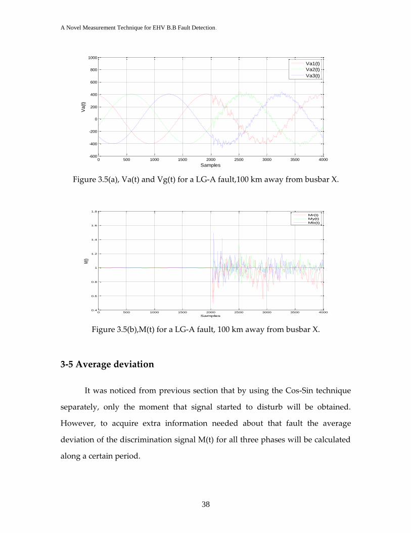
3-5 Average deviation ............................................................................................... 38

3-6 Conclusions .......................................................................................................... 40

Chapter 4 Proposed Cos-Sin Digital Relay ............................................ 41

4.1 Introduction .......................................................................................................... 41

4.2 Simulation ............................................................................................................. 41

4-3 Network selection ................................................................................................ 41

4.4 Line’s Configuration and Parameters ................................................................. 42

4.5 Network structure ................................................................................................ 42

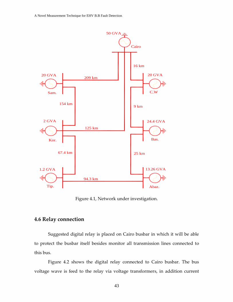
4.6 Relay connection .................................................................................................. 43

4.7 Simulation parameters ........................................................................................ 44

4.7.1 Sampling frequency ......................................................................................... 44

4.7.2 Relay operation time ........................................................................................ 45

4.8 Relay criterion: ..................................................................................................... 47

4.8.1 Fault detection criteria: .................................................................................... 47

4.8.1.1 Determination of threshold value (ζ): ....................................................... 49

4.7.2 Fault analysis criteria ....................................................................................... 52

4.8.3 Fault discrimination criteria ............................................................................. 55

4.8.3.1 Travelling waves ....................................................................................... 56

4-9 Flow Chart of the Multifunction Digital Relay ............................................... 63

Chapter 5 Simulated System Studies ...................................................... 65

5-1 Introduction .......................................................................................................... 65

5-2 Examined grid ...................................................................................................... 65

5-3 Simulated fault cases ........................................................................................... 66

5-3-1 Fault location ................................................................................................... 66

5-3-2 Fault Type ....................................................................................................... 66

5-3-3 Fault Resistance............................................................................................... 67

5-3-4 Fault inception angle ....................................................................................... 67


V

5-4 Case By Case Study ............................................................................................. 67

5-4-1 Busbar fault ..................................................................................................... 69

5-4-1-1 L-G B.B fault ........................................................................................... 69

A) R=0 Ω .......................................................................................................... 69

B) R=10 Ω......................................................................................................... 70

5-4-1-2 L-L-G B.B fault ....................................................................................... 72

A) R=0 Ω .......................................................................................................... 72

B) R=10 Ω......................................................................................................... 73

5-4-1-3 L-L B.B fault ............................................................................................ 75

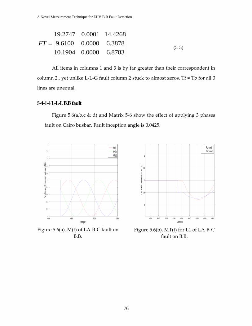
5-4-1-4 L-L-L B.B fault ........................................................................................ 76

5-4-2 Line faults ........................................................................................................ 77

5-4-2-1 L-G Line fault .......................................................................................... 78

5-4-2-3 L-L-G Line fault ...................................................................................... 79

5-4-2-3 L-L Line fault ........................................................................................... 81

5-4-2-4 L-L-L Line fault ....................................................................................... 82

5-4-3 Farther distance fault ....................................................................................... 84

5-4-3-1 L-G Long line fault .................................................................................. 84

A) R=0 Ω .......................................................................................................... 84

B) R=10 Ω......................................................................................................... 86

5-4-3-2 L-L-G Long line fault .............................................................................. 87

5-4-3 Special fault cases ........................................................................................... 89

5-4-3-1 Very close faults ...................................................................................... 89

A) L-G closed faults, R=0 ohm ........................................................................ 89

B) L-G closed faults ,R=10 ohm ....................................................................... 91

5-4-3-2 High fault resistance ................................................................................ 92

A) B.B L-G fault with high resistance. ............................................................. 92

B) Transmission line L-G fault with high resistance. ....................................... 94

5-4-3-2 Critical inception angles. ......................................................................... 95

A) B.B L-G fault at inception in peak point. .................................................... 95

B) B.B L-G fault at inception in zero crossing point. ....................................... 97

C) Line L-G fault at inception in peak point..................................................... 98

D) Line L-G fault at inception in zero crossing point. .................................... 100

5-5 Summary: ............................................................................................................ 101

Chapter 6 Practical Relay Application Over a Lab Model ................ 103

5-1 Introduction ........................................................................................................ 103

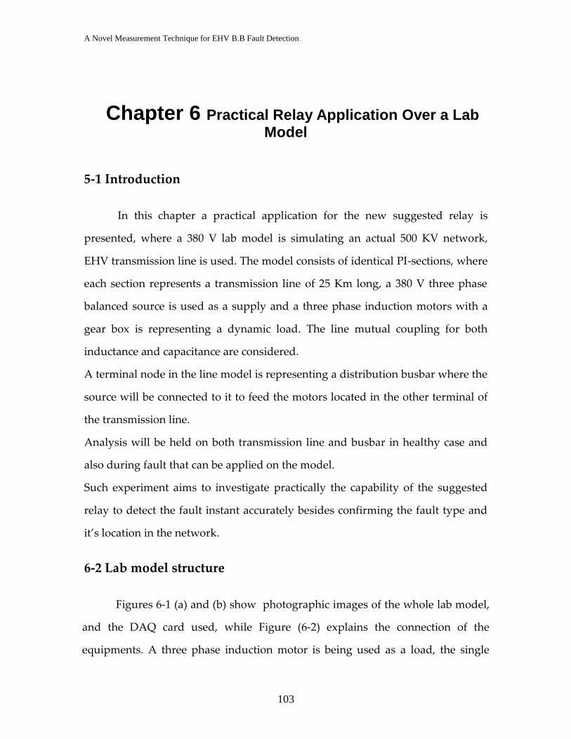
6-2 Lab model structure .......................................................................................... 103

6-2-1 Normal Operation .......................................................................................... 106

6-2-2 Fault conditions ............................................................................................. 108

6-2-2-1 Busbar fault ............................................................................................ 108

6-2-2-2 Line fault ................................................................................................ 109

6-2-3 Practical modeling for fault discrimination criteria ...................................... 111

6-2-3-1 No fault .................................................................................................. 111

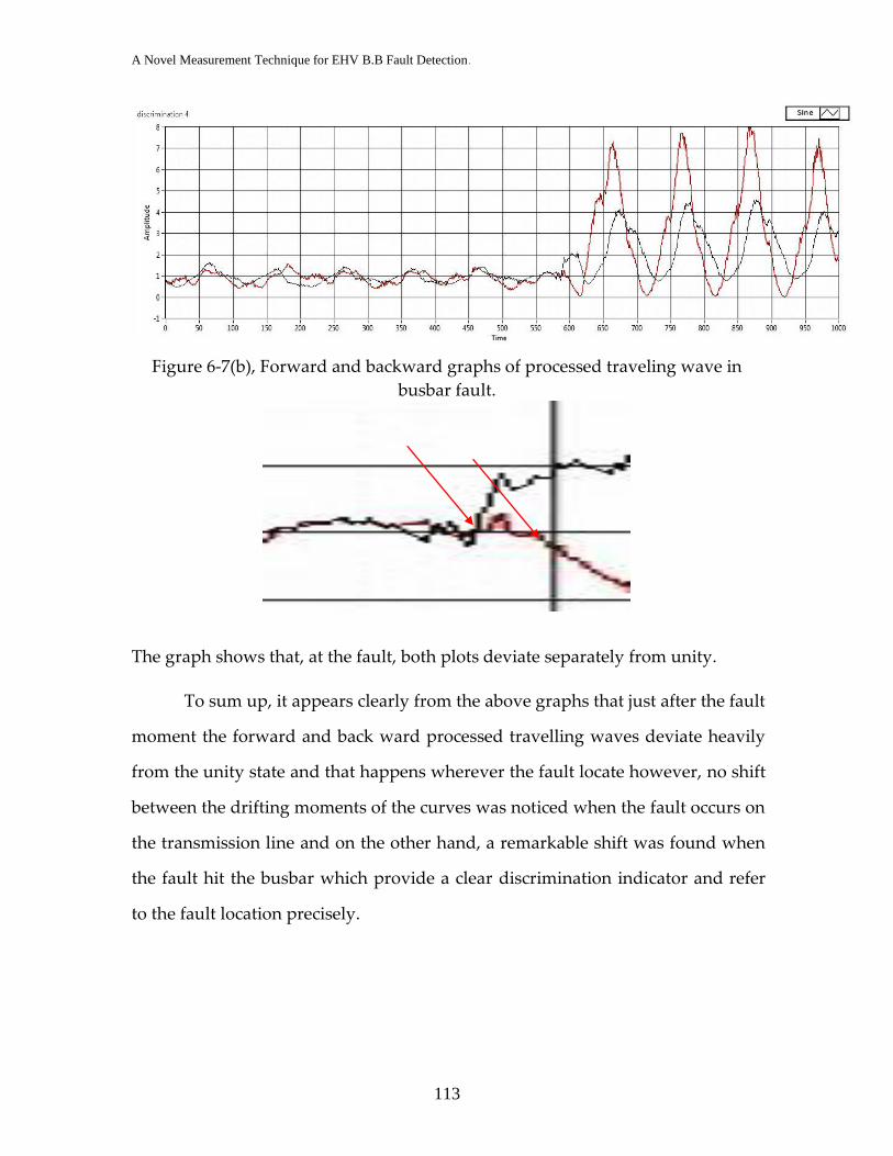
6-2-3-2 fault condition ........................................................................................ 112

6-3 Conclusion .......................................................................................................... 114

Chapter 7 CONCLUSION ...................................................................... 115


VI

7.1 Conclusions and contributions ........................................................................ 115

7.2 Future work ........................................................................................................ 117

References ................................................................................................................. 119

Appendix [A] ............................................................................................................ 123

Typical Line Configuration and Parameters ........................................................... 123

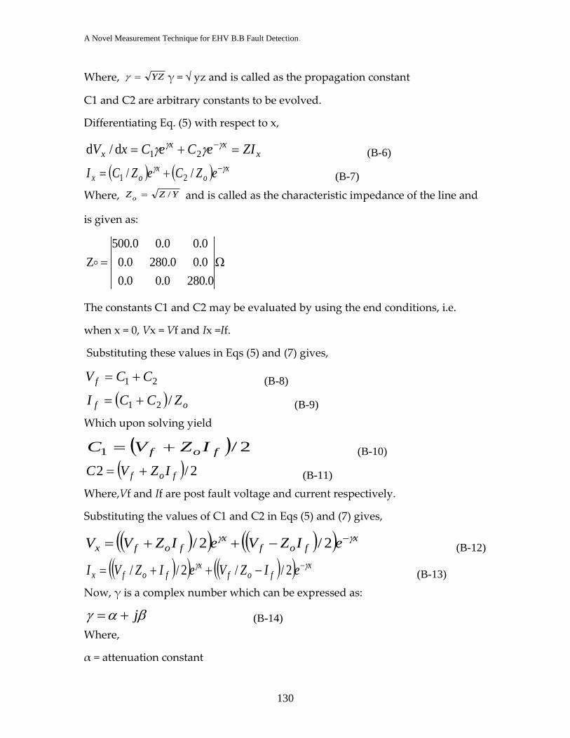
Appendix [B] ............................................................................................................ 128

Travelling waves equations..................................................................................... 128

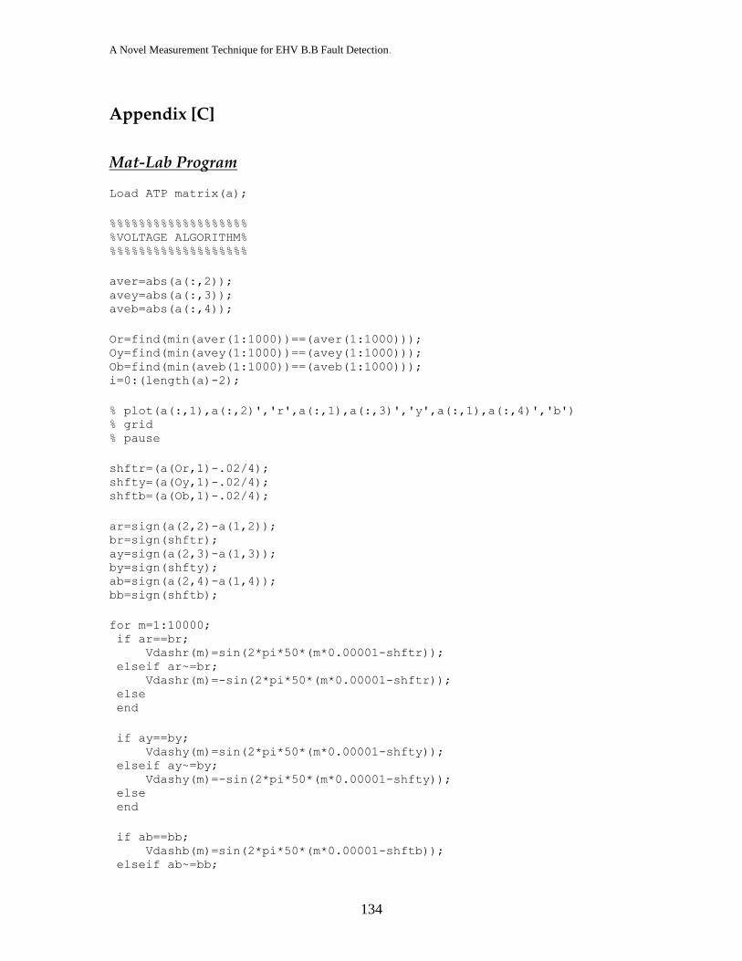
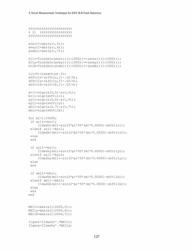
Appendix [C] ............................................................................................................ 134

Mat-Lab Program .................................................................................................... 134

Appendix [D] ............................................................................................................ 145

ATP ......................................................................................................................... 145

Appendix [E] ............................................................................................................ 147

Lab-Veiw ................................................................................................................ 147


VII

FIGURES

Figure ‎1.1, Single line diagram of power system. ....................................................... 1

Figure ‎1.2, Protection system components. .................................................................. 5

Figure ‎2.1, Single bus–single breaker. ......................................................................... 20

Figure ‎2.2, Double bus with bus tie–single breaker. ................................................. 20

Figure ‎2.3, Main and transfer bus–single breaker. .................................................... 20

Figure ‎2.4, Double bus–single breaker. ....................................................................... 20

Figure ‎2.5, Double bus–double breaker. ..................................................................... 20

Figure ‎2.6, Ring bus. ...................................................................................................... 20

Figure ‎2.7, Breaker- and-a-half bus. ............................................................................ 21

Figure ‎2.8, Frame earth protection arrangement. ...................................................... 24

Figure ‎2.9, Differential protection basic connection. ................................................ 25

Figure ‎2.10, Over-current differential protection. ..................................................... 26

Figure ‎2.11, Multi-restraint Differential Relay. .......................................................... 27

Figure ‎2.12, High impedance differential protection. ............................................... 28

Figure ‎2.13, Directional comparison. .......................................................................... 29

Figure ‎2.14, Digital protection. ..................................................................................... 30

Figure ‎3.1, Va(t) and Vg(t) signals for one phase during LG fault. ........................ 33

Figure ‎3.2, 500 KV sample network. ............................................................................ 35

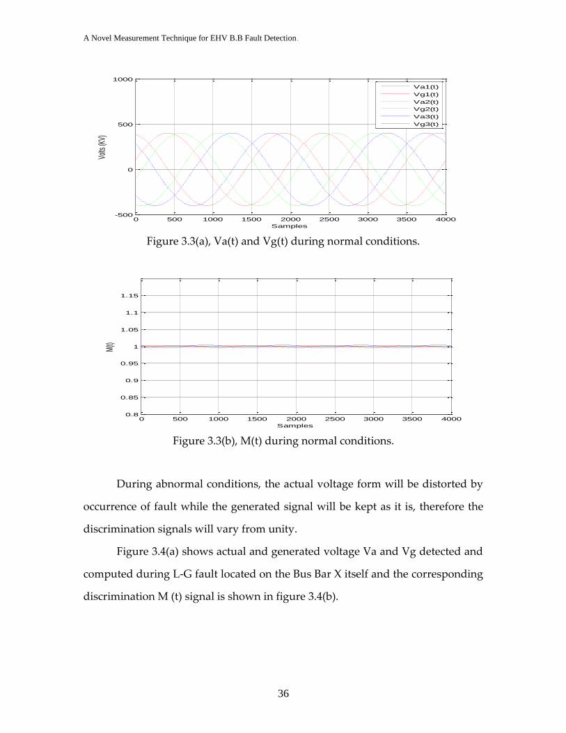
Figure ‎3.3(a), Va(t) and Vg(t) during normal conditions. ........................................ 36

Figure ‎3.3(b), M(t) during fault conditions. ............................................................... 36

Figure ‎3.4(a), Va(t)and Vg(t) for a LG-A fault on busbar X. .................................... 36

Figure ‎3.4(b), M(t) for a LG-A fault on busbar X. ...................................................... 36

Figure ‎3.5(a), Va(t) and Vg(t) for a LG-A fault,100 KM away from busbar X. ...... 36

Figure ‎3.5(b), M(t) for a LG-A fault, 100 KM away from busbar X. ....................... 36

Figure 4.1, Under investigation network.................................................................... 43

Figure 4.2, Tool DSP connection. ................................................................................. 44

Figure 4.3, Pre-fault and post fault cycles under operation. ................................... 45

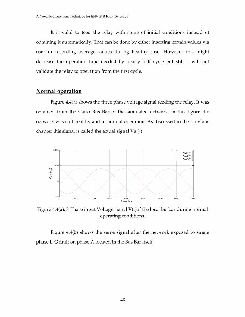
Figure 4.4(a), 3-Ø i/p voltage V(t) of the local busbar during normal case. .......... 46

Figure 4.4(b), 3-Ø i/p voltage V(t) of the local busbar during L-G fault case. ....... 47

Figure 4.5, Ripples in unity discrimination. ............................................................... 49

Figure 4.6, Errors in point detection............................................................................ 50

Figure 4.7(a), M(t) unity relation in normal case and the threshold limits. ........... 52

Figure 4.7(b), M(t) unity relation in fault case and the threshold limits. ............... 52

Figure 4.8, All lines connection to the relay. .............................................................. 55

Figure 4.9(a), Travelling waves lattice diagram during line1 fault. ....................... 58

Figure 4.9(b), Travelling waves lattice diagram during line2 fault. ....................... 59


VIII

Figure 4.9(c), Travelling waves lattice diagram during busbar fault. .................... 60

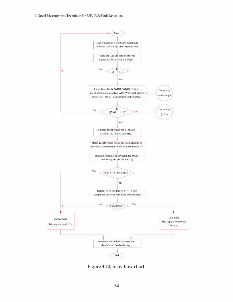
Figure 4.10, Relay flow chart. ....................................................................................... 64

Figure 5.1(a), M(t) of LA-G fault on B.B with R≈0 Ω ................................................... 69

Figure 5.1(b), MT(t) for L1 of LA-G fault on B.B with R≈0 Ω ..................................... 69

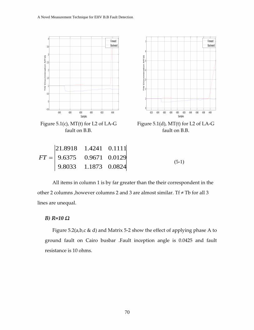
Figure 5.1(c), MT(t) for L2 of LA-G fault on B.B with R≈0 Ω ...................................... 70

Figure 5.1(d), MT(t) for L3 of LA-G fault on B.B with R≈0 Ω ...................................... 70

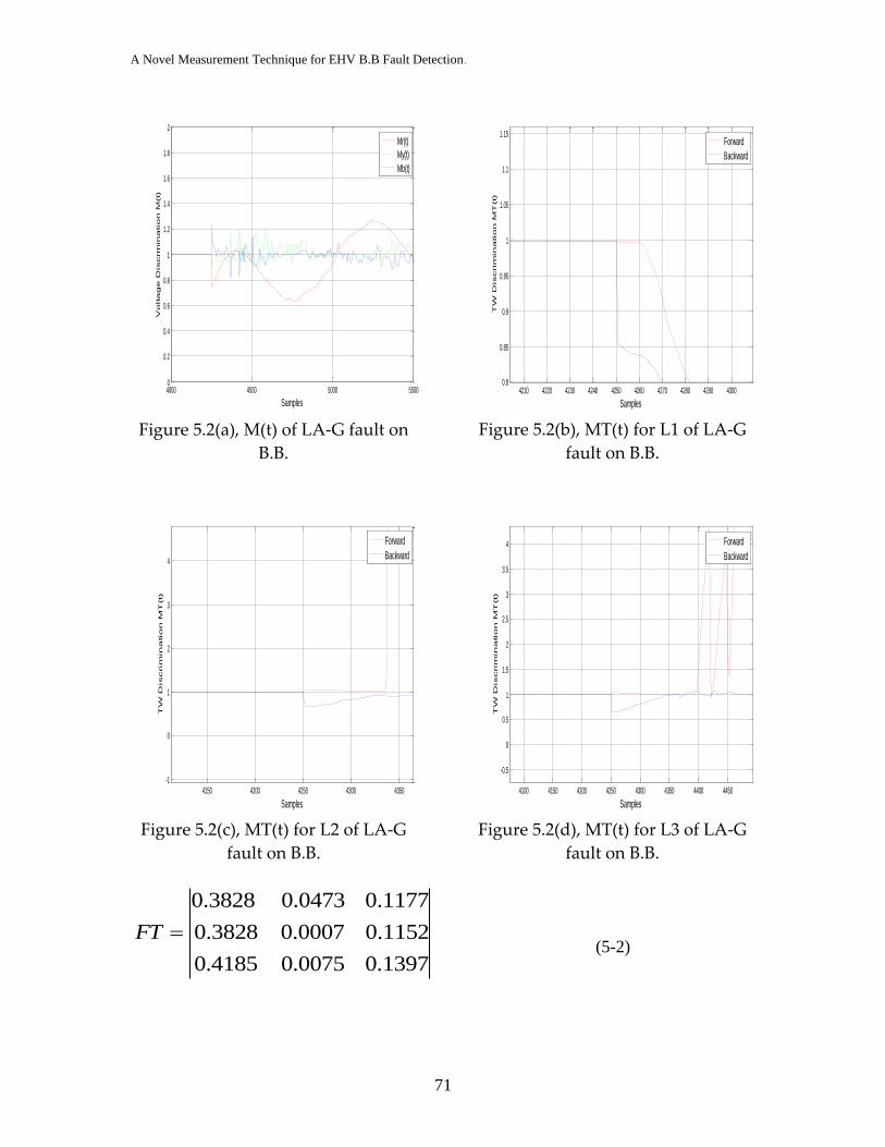
Figure 5.2(a), M(t) of LA-G fault on B.B with R≈10 Ω ................................................. 71

Figure 5.2(b), MT(t) for L1 of LA-G fault on B.B with R≈10 Ω ................................... 71

Figure 5.2(c), MT(t) for L2 of LA-G fault on B.B with R≈10 Ω .................................... 71

Figure 5.2(d),‎MT(t) for L3 of LA-G fault on B.B with R≈10 Ω .................................... 71

Figure 5.3(a), M(t) of LA-C-G fault on B.B with R≈0 Ω ............................................... 72

Figure 5.3(b), MT(t) for L1 of LA-C-G fault on B.B with R≈0 Ω ................................. 72

Figure 5.3(c), MT(t) for L2 of LA-C-G fault on B.B with R≈0 Ω .................................. 73

Figure 5.3(d), MT(t) for L3 of LA-C-G fault on B.B with R≈0 Ω ................................. 73

Figure 5.4(a), M(t) of LA-C-G fault on B.B with R≈10 Ω ............................................. 74

Figure 5.4(b), MT(t) for L1 of LA-C-G fault on B.B with R≈10 Ω ............................... 74

Figure 5.4(c), MT(t) for L2 of LA-C-G fault on B.B with R≈10 Ω ................................ 74

Figure 5.4(d), MT(t) for L3 of LA-C-G fault on B.B with R≈10 Ω ............................... 74

Figure 5.5(a), M(t) of LA-C fault on B.B ....................................................................... 75

Figure 5.5(b), MT(t) for L1 of LA-C fault on B.B .......................................................... 75

Figure 5.5(c), MT(t) for L2 of LA-C fault on B.B .......................................................... 75

Figure 5.5(d), MT(t) for L3 of LA-C fault on B.B ......................................................... 75

Figure 5.6(a), M(t) of LA-B-C fault on B.B ................................................................... 76

Figure 5.6(b), MT(t) for L1 of LA-B-C fault on B.B ...................................................... 76

Figure 5.6(c), MT(t) for L2 of LA-B-C fault on B.B ...................................................... 77

Figure 5.6(d), MT(t) for L3 of LA-B-C fault on B.B ..................................................... 77

Figure 5.7(a), M(t) of LA-G fault on L2 with R≈0 Ω ..................................................... 78

Figure 5.7(b), MT(t) for L1 of LA-G fault on L2 with R≈0 Ω ....................................... 78

Figure 5.7(c), MT(t) for L2 of LA-G fault on L2 with R≈0 Ω ........................................ 79

Figure 5.7(d), MT(t) for L3 of LA-G fault on L2 with R≈0 Ω ....................................... 79

Figure 5.8(a), M(t) of LA-C-G fault on L2 with R≈0 Ω ................................................. 80

Figure 5.8(b), MT(t) for L1 of LA-C-G fault on L2 with R≈0 Ω ................................... 80

Figure 5.8(c), MT(t) for L2 of LA-C-G fault on L2 with R≈0 Ω .................................... 80

Figure 5.8(d), MT(t) for L3 of LA-C-G fault on L2 with R≈0 Ω ................................... 80

Figure 5.9(a), M(t) of LA-C fault on L2 ......................................................................... 81

Figure 5.9(b), MT(t) for L1 of LA-C fault on L2 ............................................................ 81

Figure 5.9(c), MT(t) for L2 of LA-C fault on L2 ............................................................ 82

Figure 5.9(d), MT(t) for L3 of LA-C fault on L2 ........................................................... 82

Figure 5.10(a), M(t) of LA-B-C fault on L2 ................................................................... 36

Figure 5.10(b), MT(t) for L1 of LA-B-C fault on L2...................................................... 83


IX

Figure 5.10(c), MT(t) for L2 of LA-B-C fault on L2 ...................................................... 83

Figure 5.10(d), MT(t) for L3 of LA-B-C fault on L2 ..................................................... 83

Figure 5.11(a), M(t) of LA-G fault on L3 (long line) with R≈0 Ω ................................. 85

Figure 5.11(b), MT(t) for L1 of LA-G fault on L3 (long line) with R≈0 Ω ................... 36

Figure 5.11(c), MT(t) for L2 of LA-G fault on L3 (long line) with R≈0 Ω .................... 36

Figure 5.11(d), MT(t) for L3 of LA-G fault on L3 (long line) with R≈0 Ω ................... 36

Figure 5.12(a), M(t) of LA-G fault on L3 (long line) with R≈10 Ω ............................... 86

Figure 5.12(b), MT(t) for L1 of LA-G fault on L3 (long line) with R≈10 Ω ................. 86

Figure 5.12(c), MT(t) for L2 of LA-G fault on L3 (long line) with R≈10 Ω .................. 87

Figure 5.12(d), MT(t) for L3 of LA-G fault on L3 (long line) with R≈10 Ω ................. 87

Figure 5.13(a), M(t) of LA-C-G fault on L3 (long line) with R≈10 Ω ........................... 88

Figure 5.13(b), MT(t) for L1 of LA-C-G fault on L3 (long line) with R≈10 Ω ............. 88

Figure 5.13(c), MT(t) for L2 of LA-C-G fault on L3 (long line) with R≈10 Ω .............. 88

Figure 5.13(d), MT(t) for L3 of LA-C-G fault on L3 (long line) with R≈10 Ω ............. 88

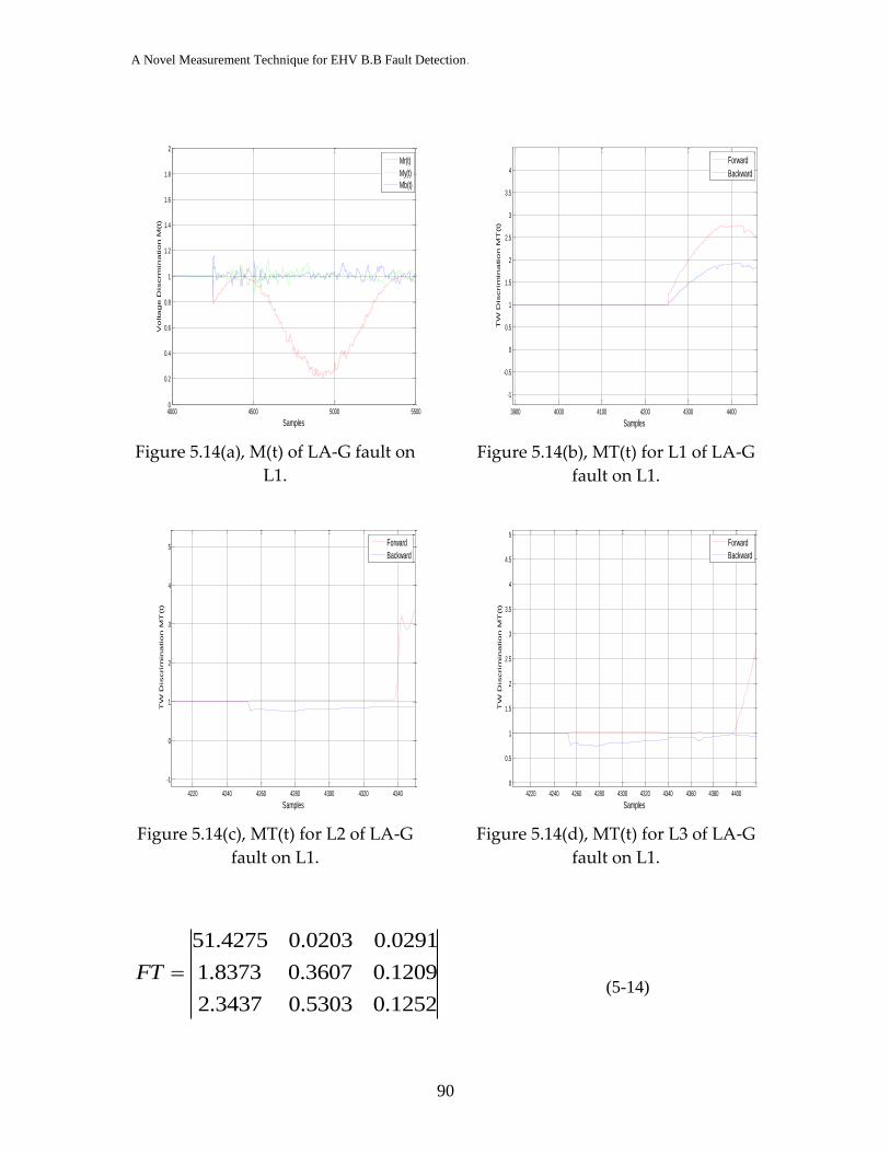
Figure 5.14(a), M(t) of LA-G fault on L1 (closed fault) with R≈0 Ω ............................. 90

Figure 5.14(b), MT(t) for L1 of LA-G fault on L1 (closed fault) with R≈0 Ω ............... 90

Figure 5.14(c), MT(t) for L2 of LA-G fault on L1 (closed fault) with R≈0 Ω ............... 90

Figure 5.14(d), MT(t) for L3 of LA-G fault on L1 (closed fault) with R≈0 Ω ............... 90

Figure 5.15(a), M(t) of LA-G fault on L1 (closed fault) with R≈10 Ω ........................... 91

Figure 5.15(b), MT(t) for L1 of LA-G fault on L1 (closed fault) with R≈10 Ω ............. 91

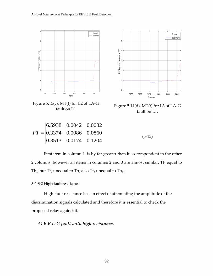
Figure 5.15(c), MT(t) for L2 of LA-G fault on L1 (closed fault) with R≈10 Ω ............. 92

Figure 5.15(d), MT(t) for L3 of LA-G fault on L1 (closed fault) with R≈10 Ω ............. 92

Figure 5.16(a), M(t) of LA-G fault on B.B with R≈100 Ω (HI resistance) .................... 93

Figure 5.16(b), MT(t) for L1 of LA-G fault on B.B with R≈100 Ω (HI resistance) ....... 93

Figure 5.16(c), MT(t) for L2 of LA-G fault on B.B with R≈100 Ω (HI resistance) ....... 93

Figure 5.16(d), MT(t) for L3 of LA-G fault on B.B with R≈100 Ω (HI resistance) ...... 93

Figure 5.17(a), M(t) of LA-G fault on L2 with R≈100 Ω (HI resistance) ...................... 94

Figure 5.17(b), MT(t) for L1 of LA-G fault on L2 with R≈100 Ω (HI resistance) ......... 94

Figure 5.17(c), MT(t) for L2 of LA-G fault on L2 with R≈100 Ω (HI resistance) ......... 95

Figure 5.17(d), MT(t) for L3 of LA-G fault on L2 with R≈100 Ω (HI resistance) ........ 95

Figure 5.18(a), M(t) of LA-G fault on B.B with R≈0 Ω (peak inception angle) ............ 96

Figure 5.18(b), MT(t) for L1 of LA-G fault on B.B with R≈0 Ω (peak inception angle)96

Figure 5.18(c), MT(t) for L2 of LA-G fault on B.B with R≈0 Ω (peak inception angle) 96

Figure 5.18(d), MT(t) for L3 of LA-G fault on B.B with R≈0 Ω (peak inception angle)

........................................................................................................................................... 96

Figure 5.19(a), M(t) of LA-G fault on B.B with R≈10 Ω (zero crossing angle) ............. 97

Figure 5.19(b), MT(t) for L1 of LA-G fault on B.B with R≈10 Ω (zero crossing angle) 97

Figure 5.19(c), MT(t) for L2 of LA-G fault on B.B with R≈10 Ω (zero crossing angle) 98

Figure 5.19(d), MT(t) for L3 of LA-G fault on B.B with R≈10 Ω (zero crossing angle)98

Figure 5.20(a), M(t) of LA-G fault on L2 with R≈0 Ω (peak inception angle) .............. 99


X

Figure 5.20(b), MT(t) for L1 of LA-G fault on L2 with R≈0 Ω (peak inception angle) 99

Figure 5.20(c), MT(t) for L2 of LA-G fault on L2 with R≈0 Ω (peak inception angle) . 99

Figure 5.20(d), MT(t) for L3 of LA-G fault on L2 with R≈0 Ω (peak inception angle) 99

Figure 5.21(a), M(t) of LA-G fault on L2 with R≈0 Ω (zero crossing angle) .............. 100

Figure 5.21(b), MT(t) for L1 of LA-G fault on L2 with R≈0 Ω (zero crossing angle) . 100

Figure 5.21(c), MT(t) for L2 of LA-G fault on L2 with R≈0 Ω (zero crossing angle) . 101

Figure 5.21(d), MT(t) for L3 of LA-G fault on L2 with R≈0 Ω (zero crossing angle) 101

Figure 6.1(a), 380 V lab model for 500 KV Transmission line .................................... 104

Figure 6.1(b), NI-Interface card used in Lab ............................................................ 104

Figure 6.2, Lab equipment connection ...................................................................... 105

Figure 6.3(a), Input phase voltage and complementary generated signal during

normal conditions. ....................................................................................................... 106

Figure 6.3(b), System 3 phase current signal during normal conditions ............. 107

Figure 6.3(c), Discrimination signal resulting from applying the Cos- Sin

technique ....................................................................................................................... 107


busbar fault conditions ................................................................................................ 108

Figure 6.4(b), Discrimination signal resulting from busbar fault ......................... 109


line fault conditions ..................................................................................................... 110

Figure 6.5(b), Discrimination signal resulting from line fault ............................... 110

Figure 6.6, Forward and backward graphs of processed traveling wave in no

fault condition .............................................................................................................. 111

Figure 6.7(a), Forward and backward graphs of processed traveling wave in

transmission line fault ................................................................................................. 112

Figure 6.7(b), Forward and backward graphs of processed traveling wave in

busbar fault ................................................................................................................... 113


XI

TABLES

Table ‎2.1, Advantages and disadvantages of bus arrangement .............................. 22

Table ‎3.1, Average deviation due to LG faults at phase A on the busbar X & Line

XY. .................................................................................................................................... 39

Table ‎4.1, Nodes of the selected grid. .......................................................................... 42

Table ‎5.1, Travelling waves timing scenarios followed to detect fault place. ....... 68

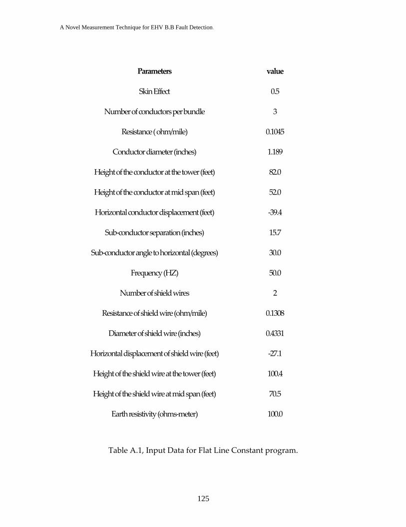
Table A.1, Input Data for Flat Line Constant program. ......................................... 125

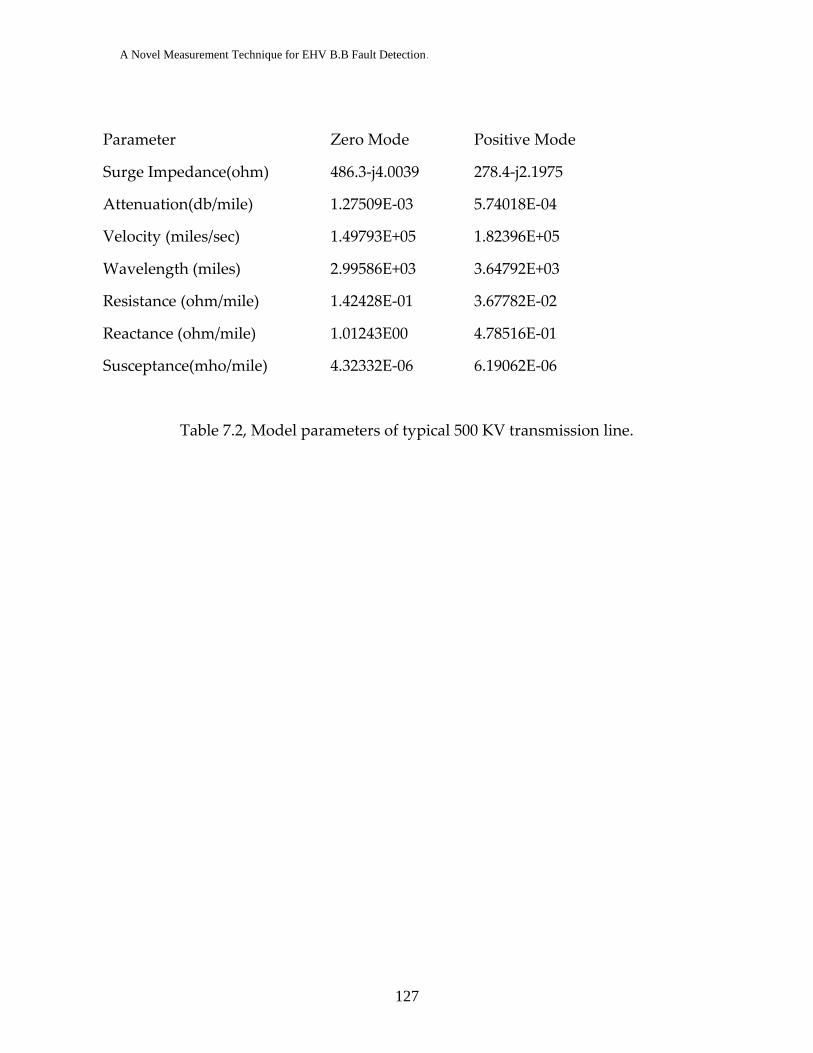
Table ‎A.2, Model parameters of typical 500 KV transmission line. ...................... 127


1

Chapter 1 Introduction

1.1 Background:

An electric power system comprises of generation, transmission and

distribution of electric energy [1]. They allow for power to be generated

(generators), transformed from one voltage level to another (transformers),

transmitted from one location to another (transmission lines), distributed among

a number of transmission lines and power transformers (busses), and used by

consumers (loads) [2].

Figure 1.1 is a one line graphical representation of the power system, the

dashed borders contains the protective zones that covers one or at most two

elements of the power system. The protective zones are planned in overlapped

way that entire power system is collectively covered by them, and thus, no part

of the system is left unprotected [3].

Figure ‎1.1, Single line diagram of power system.


2

Usually power system operates in steady state to deliver customers with

convenient energy in proper voltage waveform and designated frequency. In up

normal operation, system subjects to disturbances that caused by either heavy

load changes or by the effect of a fault.

A fault in electric equipment is defined as a defect in its electrical circuit

due to which the current is diverted from the intended path. Faults are generally

caused by breaking of the conductor or failure of insulation. The other reasons

include mechanical failure, accident, excessive internal end external stress, aging,

operator mistakes---etc.[4].

On the occurrence of faults, current is relatively high so the fault currents

can damage the defected equipment, system three phase voltage become un

balanced ,faulted phase voltage decreases, power flow is directed towards the

fault and the supply to the neighboring zone is effected [5].

Although proper power system planning and using sophisticated well

fabricated component can minimized faults yet they can never prevent it

completely therefore, it is necessary to protect power systems from faults.

1.2 Power system protection:

System protection is the actions taken to make sure that faults caused by

abnormal operating conditions are detected and the affected part of the system is

quickly removed from operation [6].

Modern power system evolves large amount of investment nowadays, so

it is very important to avoid damages might happened to equipment of the

utility as they take much time and cost to repair. Also service failure of a large


3

portion of the system is not acceptable. It is significant to keep the impaired

component and the isolated part as minimum as possible.

1.2.1 Parameters of protective system

Protective system should have certain Parameters that are very important

and should be considered [7]. The qualities of the protective systems are named

as:

Reliability: assurance that the protection will perform correctly.

Selectivity: maximum continuity of service with minimum system disconnection.

Speed of operation: minimum fault duration and consequent equipment damage

and system instability.

Simplicity: minimum protective equipment and associated circuitry to achieve

the protection objectives.

Economics: maximum protection at minimal total cost knowing that a better

protective system costs more.

1.2.1.1 Reliability

Reliability has two aspects, dependability and security. Dependability is

defined as ‘‘the degree of certainty that a relay or relay system will operate

correctly’’ (IEEE C 37.2). Security ‘‘relates to the degree of certainty that a relay or

relay system will not operate incorrectly’’ (IEEE C 37.2). In other words,

dependability indicates the ability of the protection system to perform correctly

when required, whereas security is its ability to avoid unnecessary operation

during normal day after-day operation, and faults and problems outside the

designated zone of operation.


4

1.2.1.2 Selectivity-Coordination

Relays have an assigned area known as the primary protection zone, but

they may properly operate in response to conditions outside this zone. In these

instances, they provide backup protection for the area outside their primary

zone. This is designated as the backup or overreached zone. Selectivity (also

known as relay coordination) is the process of applying and setting the

protective relays that overreach other relays such that they operate as fast as

possible within their primary zone, but have delayed operation in their backup

zone.

1.2.1.3 Speed

System should operate promptly interrupting the designated zone when it

is required to do so to minimize the damages on the faulted equipment and

provide the most possible human safety. Although speed action is inherently

desired, sometimes where coordination quality engaged very fast or zero delay

operation can cause of false tripping and losing of security. In general the faster

the operation, the higher the probability of incorrect operation.

1.2.1.4 Sensitivity

Sensitivity in protective systems is the ability of the system to identify an

abnormal condition that exceeds a nominal "pickup" or detection threshold value

and which initiates protective action when the sensed quantities exceed that

threshold.


5

1.2.1.5 Economics

It is fundamental to obtain the maximum protection for the minimum

cost, and cost is always a major factor however we can’t ignore the fact that a

better protective system costs more.

1.2.2 Elements of a protection system

Although, in common usage, a protection system may mean only the

relays, the actual protection system consists of many other subsystems which

contribute to the detection and removal of faults. As shown in Figure 1.2, the

major subsystems of the protection system are the transducers, relays, battery

and circuit breakers. The transducers, i.e. the current and voltage transformers,

constitute a major component of the protection system. Relays are the logic

elements which initiate the tripping and closing operations, and we will, of

course, discuss relays in the next section.

Figure ‎1.2, Protection system components.


6

1.3 Relays:

Protective relays can be classified into various ways depending on their

scheme such as over current protection, distance protection, differential

protection or it can be classified according to their function like over current,

under voltages, impedance relays [8]. In the following categorization the

classification of protective relays based on technology.

1. Electromagnetic Relays.

2. Static Relays.

3. Digital Relays.

4. Numerical relays.

In the previous century, protective relays have gone through major

transitions with the change in technology. Electromechanical relays, the oldest in

the family of protective relays, served the power system quite reliably. With the

development in electronics, solid-state relays were developed. Small size, light

weight and quiet operation are the advantages of solid-state relays over the

electromechanical relays. Microprocessors technology made the relays even more

compact, multifunctional and flexible.

1.3.1 Electromechanical relays

These relays were the earliest forms of relay used for the protection of

power systems, and they date back nearly 100 years. They work on the principle

of a mechanical force causing operation of a relay contact in response to a

stimulus. The mechanical force is generated through current flow in one or more

windings on a magnetic core or cores, hence the term electromechanical relay.


7

1.3.2 Solid-State Relays

Solid-state or static relays began in the early 1960’s.they are

semiconductor devices composed of electronic components like resistors, diodes,

transistors…etc. These relays do not have moving parts which make them lighter

and smaller than electromagnetic relays. Solid-state relays perform the same

functions as electromagnetic relays except that they need less voltage to operate

and switching can be performed in very short times.

1.3.3 Digital relays

Microprocessors and microcontrollers replaced analogue circuits used in

static relays to implement relay functions. Early examples began to be introduced

into service around 1980, and, with improvements in processing capacity, can

still be regarded as current technology for many relay applications. However,

such technology will be completely superseded within the next five years by

numerical relays. Digital relays introduce A/D conversion of all measured

analogue quantities and use a microprocessor to implement the protection

algorithm. The microprocessor may use some kind of counting technique, or use

the Discrete Fourier Transform (DFT) to implement the algorithm. However, the

typical microprocessors used have limited processing capacity and memory

compared to that provided in numerical relays. The functionality tends therefore

to be limited and restricted largely to the protection function itself.

1.3.4 Numerical relays

The difference between digital and numerical relay can be viewed as

natural developments of digital relays as a result of advances in technology.

Typically, they use a specialized digital signal processor (DSP) as the

computational hardware, together with the associated software tools. The input


8

analogue signals are converted into a digital representation and processed

according to the appropriate mathematical algorithm.

1.4 Fault Detection based on Transient Analysis Techniques

Fault detection using fault transient analysis has been successfully applied

as a scheme on extra high-voltage protection. Fault transient signals are high

frequency signals superimposed on the steady state voltage and currents. The

transient signals hold plenty of useful information regarding the fault that can

help in detecting all its parameters; they can then be extracted from the power

frequency signals by applying a suitable tool. A number of methods are available

for transient analysis; these methods can be categorized as time domain methods,

frequency domain or time frequency domain [9, 10].

1.4.1 Time Domain Approach

There have been a lot of attempts to determine the fault occurrence using

signal analysis in the time domain because of its simplicity. In this section, a

review of some of these techniques is presented.

1.4.1.1 Statistical Analysis

The objective of signal feature extraction is to represent the signal in terms

of a set of properties or parameters. The most common measurements in

statistics are the arithmetic mean, standard deviation, and variance. All these

parameters actually compute the value about which the data are centered. In fact,

all measures of central tendency may be considered estimates of mean. The

arithmetic mean of a sample may be computed as:


9

n

i

ixn

x

1

1 (1.1)

Where: xi is the samples signal, x is the signal mean and n is the number of

samples.

The standard deviation measures the dispersion of set of samples. It is

most often measured by the deviation of the samples from their average. The

sum of these deviations will be zero and the sum of squares of the deviations is

positive. The standard deviation of a sample is computed as:

n

i

i xxn

s1

2

1

1

(1.2)

The variance is the average of the squared deviations as in the form:

n

i

i xxn

s1

22

1

1

(1.3)

Another important parameter in statistical estimation method is called the

auto correlation coefficient, which measures the correlation between samples at

different distance apart. It is closely related to convolution and, when applied to

signals, provides a method of measuring the "similarity" between corresponding

signals. The concept of cross-correlation analysis (CCA) is similar to ordinary

correlation coefficient, namely that given N pairs of samples on two variables x

and y, the correlation coefficient is given by

yyxxn

R tk

n

k

tk

1

xy

1

(1.4)


10

Where xyR is the cross correlation function of the signals x and y, n is the number

of samples, x is x mean, y is y mean and ∆t is sampling interval. The mean is

removed to attenuate any exponential or power frequency signal. Correlation is a

common operation in many signal processing techniques.

1.4.1.2 Signal Derivative

The use of the first derivative of the current or voltage signals has been

reported since a long time. This kind of filtering is based on a data window of

two samples for extracting the abrupt changes of the monitored signal. The first

differences of the current samples can be expressed as:

nnn III 1 (1.5)

Where In is the nth sample of the signal I.

A three sample sequence filter, which is based on the second difference of

the current samples, is considered. The second difference filter; with three

samples window; can be expressed as:

11 2 nnnn IIII (1.6)

where n is the sample number.

1.4.2 Frequency Domain Approach

Fourier transform-based fault location algorithms have been proposed for

a long time. Most of the proposed algorithms use voltages and currents between

fault initiation and fault clearing. To find out the frequency contents of the fault

signal, several transformations can be applied, namely, Fourier, wavelet, Wigner,

etc., among which the Fourier transform is the most popular and easy to use.


11

1.4.2.1 Fourier Transform

Fourier transform (FT) is the most popular transformation that can be

applied to transient signals to obtain their frequency components appearing in

the fault signal. Usually, the information that cannot be readily seen in the time

domain can be seen in the frequency domain. The FT and its inverse give a one-

to-one relationship between the time domain x(t) and the frequency domain

X(ω).

Given a signal I(t), the Fourier Transform FT(ω) is defined by the

following equation:

dtetIFT tj

.)( )( (1.7)

Where ω is the continuous frequency variable. This transform is very suitable for

stationary signal, where every frequency components occur in all time. The

discrete form of the FT can be written as

N

knjN

n

enIN

kDFT2

1

.][1

][

(1.8)

Where 1 ≤ k ≤ N.

The FT gives the frequency information of the signal, but it does not tell us

when in time these frequency components exist. The information provided by

the integral corresponds to all time instances because the integration is done for

all time intervals. It means that no matter where in time the frequency f appears,

it will affect the result of the integration equally. This is why FT is not suitable for

non-stationary signals.


12

1.4.3 Time - Frequency Domain Approach

Fourier transform assumes that the signal is stationary, but fault

superimposed signals such as travelling wave signal is always non-stationary. To

overcome this deficiency, modified method-short times Fourier transform and

Wavelet Transform allows representing the signal in both time and frequency

domain through time windowing function. The window length determines a

constant time and frequency resolution. Thus, a shorter time windowing is used

in order to capture the transient behavior of a signal; we sacrifice the frequency

resolution. The nature of the real fault signals is non-periodic; such signals

cannot easily be analyzed by conventional transforms. So, an alternative

mathematical tool- wavelet transform must be selected to extract the relevant

time-amplitude information from a signal. In the meantime, we can improve the

signal to noise ratio based on prior knowledge of the signal characteristics.

1.4.3.1 Short Time Fourier Transform

In the STFT, the signal is divided into small segments which can be

assumed to be stationary. The signal is multiplied by a window function within

the Fourier integral. If the window length is infinite, it becomes the DFT. In order

to obtain the stationarity, the window length must be short enough. Narrower

windows afford better time resolution and better stationarity, but at the cost of

poorer frequency resolution. One problem with the STFT is that one cannot

determine what spectral components exist at what points of time. One can only

know the time intervals in which certain band of frequencies exist. The STFT is

defined by following equation:

dtetWtItSTFT tj

.)().( ),(

(1.9)


13

Where I(t) is the measured signal, ω is frequency, W(t- τ ) is a window function, τ

is the translation, and t is time.

To separate the negative property of the DFT described above, the signal

is to be divided into small enough segments, where these segments (portion) of

the signal can be assumed to be stationary. These transforms can be displayed in

a three dimensional system (Amplitude of transform, frequency, time). And it is

clearly seen in time and frequency domain. To get better information in time or

frequency domain, parameters of the window can be changed. As

aforementioned, narrow windows give good time resolution, but poor frequency

resolution. Wide windows give good frequency resolution, but poor time

resolution. Thus, it is required to compromise between the time and frequency

resolutions.

1.4.3.2 Wavelet Transform

Signal-cutting problem in Fourier-based techniques are overcome in

wavelet analysis by using a fully scalable modulated window. The window is

shifted along the signal and for every location the spectrum is calculated. This

process then repeated several times with a shorter or longer window for every

cycle. Eventually a collection of time-frequency representations of the signal is

obtained with different resolutions. Due to the nature of this collection this

analysis is often called multi-resolution analysis [11, 12].

Wavelets derived from one mother wavelet which is a prototype function

by translation in space and dilation (changes of the scale and space

simultaneously).

A. Continuous Wavelet Transformation (CWT)

The mother wavelet W(t) given in the following Equation:


14

)(.1

)(,d

tW

dtWd

(1.10)

Where d stands for the dilation (scaling) parameter and τ is the translation

parameter of the mother function Wd,τ (t) to generate wavelets. The scale index

d indicates the wavelet’s width, and the location index τ gives its position. The

1/√d factor is for energy normalization at different scales. Once the mother

wavelet function is known, a CWT of a function, f(t), is given in following

Equation:

dttWtfdfCWT d

)().( ),,( , (1.11)

Where * stands for complex conjugation. Equation (1.1) shows how to

decompose a function into a set of basis functions, wavelets as represented by

Wd,τ (t), which are derived from one mother wavelet W(t).

As presented in Equation (1.11), the CWT of a function, f(t), is obtained by

continuously shifting a continuously scalable function, W(t) over f(t) and

calculating the correlation between the two. However, continuously translating

and scaling a wavelet function results in an infinite number of wavelets and

eventually leads to a redundant number of wavelet coefficients and an enormous

computational burden. In order to overcome this redundancy Discrete Wavelet

Transform is introduced.

2. Discrete Wavelet Transformation (DWT)

Discrete wavelets are not continuously scalable and translatable but they

are dilated and translated in discrete time steps. In DWT, filters of different

cutoff frequencies are utilized in order to decompose the signal at different

scales. A series of high-pass filters are repeatedly applied to a signal to extract


15

the high frequencies and another series of low-pass filters are applied to the

signal to analyze the low frequencies.

A general form of the discrete mother wavelet function used in DWT is

given in the following Equation:

)(.1

)(0

00

0

, j

j

jkj

d

dktW

jtW

(1.12)

where j and k are integers and d0 > 1 is a fixed dilation step. _0 is the translation

factor and depends on the dilation step, d0.

1.5 Thesis Objective

The following are the major objectives of the work reported in this thesis.

1. To develop a digital technique for detecting the occurrence and the

parameters of a fault on a busbar.

2. To apply the proposed protection technique on a network that is

simulated with actual parameters on the Alternating Transient

program (ATP).

3. To implement the fault detection practically using a lab model and

National Instrument (NI) logic controller and to check the

performance of the techniques.

1.6 Outline of the Thesis

This thesis is organized in seven chapters and five appendices.


16

The first chapter provides a background on the power system and basics

on high voltage protection; it also provides a brief to protective relays. Then the

chapter outlines the material presented in the thesis. In addition, digital

protection techniques using signal processing are introduced in this chapter.

The second chapter introduces the history of busbar protection besides

different connections (configuration) of it. It also presents the obsoleted and

contemporary methods that are used in bus protection.

The third chapter presents a new proposed technique which can be used

to detect bus faults. The new technique is based on Cos-Sin algorithm. The

technique is applied to a small network as a test.

The forth chapter presents extra two algorithms that helps to detect fault

type and location. One of them is based on the average of the unity obtained

from Cos-Sin technique while the other is depending on the travelling wave

phenomena. The chapter contains the complete scenarios of the operating criteria

and the final flow chart.

In the fifth chapter the implementation of a new digital relay to be used

with extra high voltage network is done. The Egyptian Unified 500 KV network

is simulated using the Alternative Transient Program (ATP), while the relays

software program is constructed using the MATLAB language. The simulation

results of different fault cases, at different fault inception angles and fault

resistances and the suggested relay responses for each one of them are also

included.

The sixth chapter introduces a 380 V lab model for a 500 KV transmission

line based on the Egyptian unified network parameters and investigated using

the Lab View program, where a high speed interface card is used. A node that is

modeling the busbar and the line model itself are practically protected using the


17

Cos-Sin and associated tools. A comparison is made between the theoretical and

practical results.

The seventh chapter presents the conclusion of the work done in the

thesis. It also provides expectations of the available future work that can be done

on the light of this thesis.


18

Chapter 2 Busbar protection

2.1 History:

Up to the mid 1930s, no wide scale efforts had been made to protect

busbars on a unit basis. Also there was reluctance in arranging one protective

equipment to cause simultaneous tripping of a large number of circuits.

Before the British Grid System was built in the early 1930s, many

undertakings ran isolated from adjacent ones, and so the power available for

busbar faults was often relatively small, and damage due to these faults was

generally not extensive.

By the late 1930s, the British Power Systems were extensively

interconnected, with a consequent increase in fault power.

A number of busbar faults occurred about this time, but due to their

relatively slow clearance from the system by overcurrent and earth-fault relays,

considerable damage resulted, especially in indoor stations.

These faults led to efforts being made to produce busbar protection in

such a form that it could be widely applied without itself being a further hazard

to the system.

Construction of the British 275 KV supergrid system began in about 1953,

by which time standard principles of busbar protection had been adopted for

outdoor switchgear at the higher voltages. At this time the emphasis was placed

on the avoidance of unwanted operations in order to give maximum security of

supply.

With the introduction of 400 KV substations in the 1960s, the transient

stability of generators became the more important consideration and this led to a


19

change of emphasis so that fast operating times and reliable operation would be

obtained for a fault occurring within the protected zone, which in this case

would be the busbars and switchgear [13].

2.2 Bus arrangements

Buses exist throughout the power system and, particularly, wherever two

or more circuits are interconnected. The number of circuits that are connected to

a bus varies widely. Bus faults can result in severe system disturbances, as high

fault current levels are typically available at bus locations and because all circuits

supplying fault current must be opened to isolate the problem. Thus, when there

are more than six to eight circuits involved, buses are often split by a circuit

breaker (bus tie), or a bus arrangement is used that minimizes the number o f

circuits, which must be opened for a bus fault. There are many bus arrangements

in service dictated by the foregoing and by the economics and flexibility of

system operation [14]. The buses are typically illustrated as:

Single bus–single breaker Figure 2.1.

Double bus with bus tie–single breaker Figure 2.2.

Main and transfer bus–single breaker Figure 2.3.

Double bus–single breaker Figure 2.4.

Double bus–double breaker Figure 2.5.

Ring bus Figure 2.6.

Breaker- and-a-half bus Figure 2.7.


20

Figure ‎2.1, Single bus–single breaker.

Figure ‎2.2, Double bus with bus tie–

single breaker.

Figure ‎2.3, Main and transfer bus–

single breaker.

Figure ‎2.4, Double bus–single

breaker.

Figure ‎2.5, Double bus–double

breaker.

Figure ‎2.6, Ring bus.


21

Figure ‎2.7, Breaker- and-a-half bus.

Table 2.1 presents a summary of advantages and disadvantages of each

bus arrangement [11].


22

Dis

advanta

ges

No o

pera

tin

g f

lexib

ility

One b

us v

oltage f

or

all

circuits

Circuit r

em

oved f

or

ma

inte

nance o

r pro

ble

ms

Circuit r

em

oved f

or

ma

inte

nance o

r pro

ble

ms

Bus t

ie b

reaker

fault t

rips b

oth

buses

Voltage r

equired o

n e

ach b

us

Bus t

ie b

reaker

pro

tectio

n s

uitable

for

each c

ircuit

Bus f

ault trip

s a

ll bre

akers

Pote

ntial fo

r err

or

Bus t

ie p

rote

ctio

n a

dapta

ble

for

all

circuits

Com

plic

ate

d (

undesirable

) sw

itchin

g o

f pro

tectio

n

Bus t

ie b

reaker

pro

tectio

n s

uitable

for

each c

ircuit

With lin

e b

reaker

bypassed d

iffe

rentia

l re

moved fro

m o

ne b

us

Bus t

ie b

reaker

fault t

rips a

ll bre

akers

Voltage r

equired for

each b

us

Pro

tectio

n in s

erv

ice d

urin

g b

reaker

ma

inte

nance

Tw

o b

reakers

per

line

Lin

e p

rote

ctio

n fro

m tw

o C

Ts

Requires lin

e s

ide v

oltage

Tw

o b

reakers

trip

for

line f

aults

Requires lin

e s

ide v

oltage

Rela

ys in

serv

ice d

urin

g b

reaker

ma

inte

nance

Lin

e f

aults t

rip

tw

o b

reakers

Local backup n

ot

applic

able

Open r

ing a

nd s

ubsequent fa

ult m

ay r

esult in

undesired s

yste

m s

epara

tio

n

Required m

ore

bre

akers

Cente

r bre

aker

serv

es t

wo lin

es

Requires lin

e s

ide v

oltage

Tw

o b

us d

iffe

rentia

l zones

Local backup n

ot

applic

able

Lin

e f

aults t

rip

tw

o b

reakers

Table

‎2.1

, A

dvanta

ges a

nd d

isadva

nta

ges o

f bus a

rran

gem

ent

1

2

3

1

2

3

1

2

3

4

1

2

3

4

5

1

2

3

4

5

1

2

3

4

5

1

2

3

4

5

6

Advanta

ges

Basic

, sim

ple

, econom

ical

One b

us v

oltage f

or

all

circuits

Tw

o p

ow

er

sourc

es to feed t

wo b

uses

One s

ourc

e lost, lo

ad tra

nsfe

rred

One b

us o

ut, p

art

ial serv

ice a

vaila

ble

One d

iffe

rentia

l zone

Only

one c

ircuit t

ransfe

rred

Bre

aker,

rela

ys tra

nsfe

rred for

ma

inte

nance, etc

.

Voltage o

nly

on m

ain

bus

Hig

h f

lexib

ility

Any lin

e o

pera

ted f

rom

either

bus

One b

us a

vaila

ble

as a

tra

nsfe

r bus

Very

hig

h f

lexib

ility

Overla

ppin

g p

rote

ctio

n z

ones

Bus f

ault d

oes n

ot in

terr

upt serv

ice

All

sw

itchin

g b

y b

reakers

Either

bus c

an b

e r

em

oved

Hig

h f

lexib

ility

Min

imum

bre

akers

Bus s

ectio

n p

art

of

line,

no b

us d

iffe

rentia

ls

Mo

re o

pera

tin

g fle

xib

ility

Bus s

ectio

n p

art

of

lines

1

2 1

2

3

1

2

3

4

1

2

3 1

2

3

4

5

1

2

3 1

2

Arr

angem

ent

Sin

gle

bre

aker,

sin

gle

bus

Double

bus w

ith b

us tie

Ma

in a

nd tra

nsfe

r bus

Sin

gle

bre

aker,

double

bus

Double

bre

aker,

double

bus

Rin

g b

us

Bre

aker

and a

half b

us

Fig

ure

2.1

2.2

2.3

2.4

2.5

2.6

2.7


23

2.3 Busbar Protection

A variety of methods have been used to implement bus protection system,

the most famous schemes are:

1. System protection used to cover busbars.

2. Frame-earth protection.

3. Differential protection.

a) Over current differential.

b) Percentage differential.

c) Linear coupler differential.

d) High impedance differential

4. Directional interlock protection.

The next sections will present each of them in details.

2.3.1 Schemes cover bus protection

Wherever overcurrent or distance schemes are used in a system

protection, busbar’s protection is implicitly covered. It is worth to say that

overcurrent protection usually applied to relatively simple distribution systems

or as a back-up protection, which gives a considerable time delay, whereas

distance protection provides cover for busbar faults in its second and possibly

subsequent zones [8].

2.3.2 Frame earth protection

The switchgear is lightly insulated from the earth. Primary of the current

transformer is connected between metal frame or enclosure of switchgear and an

earth point.


24

Concrete foundation of the switch gear together with all conduits and bolt

are insulated from earth, the resistance to earth being about 10 to 12 Ω. In the

occurrence of switchgear earth fault, the fault current will flow over through the

neutral connection consequently the ground fault relay will be energized [15].

Figure 2.8 illustrates the frame earth connection.

Figure ‎2.8, Frame earth protection arrangement.

2.3.3 Bus differential protection

Differential protection / Mertz-price is a scheme that is based on

Kirchhoff’s current law by comparing the vector sum of currents entering and

leaving the protected elements (Busbar). In healthy systems the current sum is

equal zero, once a fault happens the resultant of that sum deviates from zero and

different in currents represents the fault current [16]. Figure 2.9 presents the basic

concept of differential protection.


25

Figure ‎2.9, Differential protection basic connection.

During faults and especially external ones some problems appears such as [5, 17,

18]:

a) Difference in pilot wires lengths.

Pilot wires that connect measuring current transformers located in different

sites to the relay have different lengths and different resistance. This problem

can easily be solved by linking series resistors to the pilot wires.

b) CT ratio error.

Current transformers may have almost equal rates, yet during shot circuit, the

current increases excessively. Minor inadequacy of current transformers

created by different magnetic circuit’s characteristic or different saturation

conditions can cause false tripping.

c) Current transformer magnetic circuit saturation.

2.3.3.1 Over-current differential protection

Bus fault can be sensed by an over-current relay on the incoming circuit

using the arrangement in figure 2.10 [19]. This protection scheme is provided as a

primary protection when no other bus protection is available. In case of presence


26

of other main protection technique, over current and earth fault protection can

act as a back up protection.

Figure ‎2.10, Over-current differential protection.

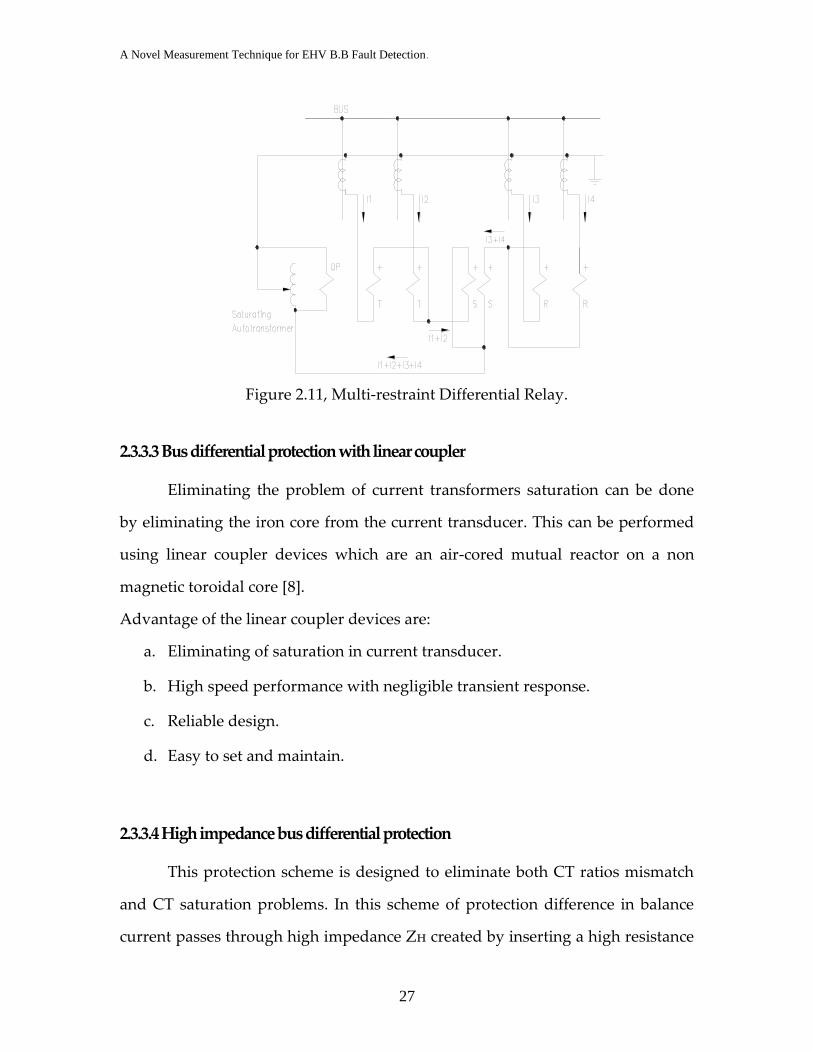
2.3.3.2 Biased / percentage differential bus zone protection:-

Percentage differential protection overcomes the problem of different CT

ratios and solves the problem of false tripping during high current values arising

from external faults.

In this relay the operating coil is connected to midpoint of a restraining

coil. The circulating current flows through restraining coils while the spill

current pass through the operating coil. For external faults, average restraining

current increases and thereby the restraining torque increases which prevents the

mal-operation of the relay. Figure 2.11 demonstrate the Connections of Multi-

restraint Differential Relay [20].


27

Figure ‎2.11, Multi-restraint Differential Relay.

2.3.3.3 Bus differential protection with linear coupler

Eliminating the problem of current transformers saturation can be done

by eliminating the iron core from the current transducer. This can be performed

using linear coupler devices which are an air-cored mutual reactor on a non

magnetic toroidal core [8].

Advantage of the linear coupler devices are:

a. Eliminating of saturation in current transducer.

b. High speed performance with negligible transient response.

c. Reliable design.

d. Easy to set and maintain.

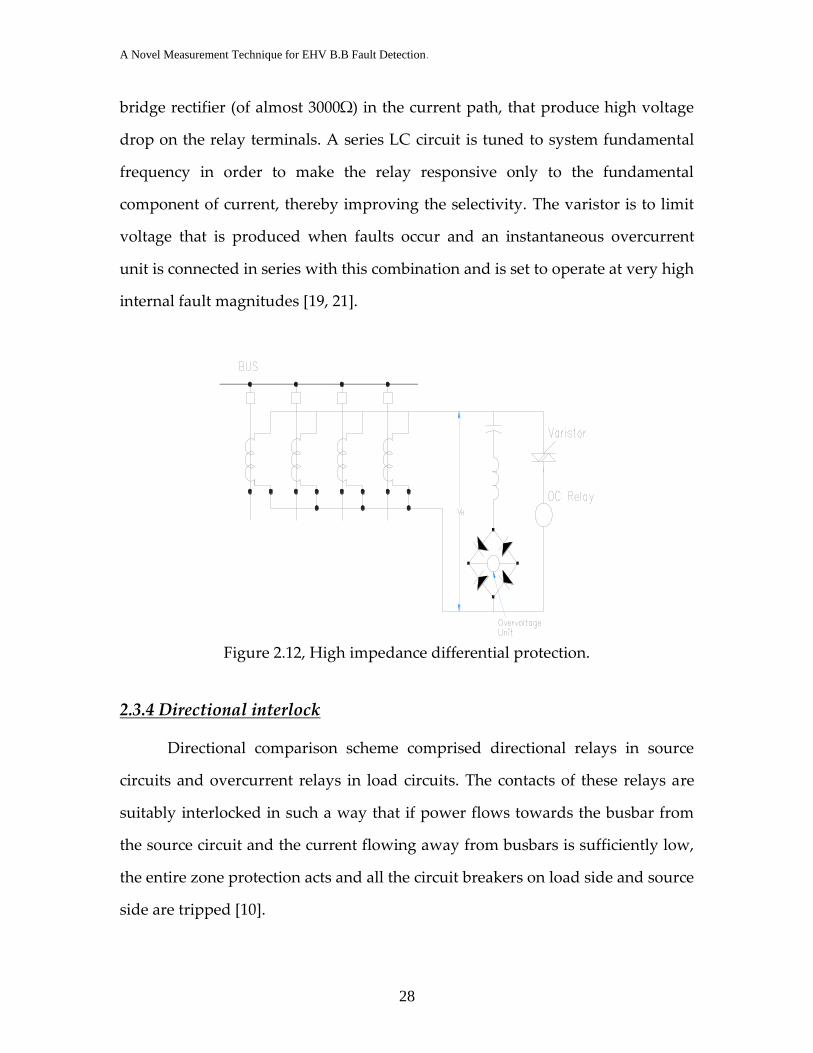
2.3.3.4 High impedance bus differential protection

This protection scheme is designed to eliminate both CT ratios mismatch

and CT saturation problems. In this scheme of protection difference in balance

current passes through high impedance Zн created by inserting a high resistance


28

bridge rectifier (of almost 3000Ω) in the current path, that produce high voltage

drop on the relay terminals. A series LC circuit is tuned to system fundamental

frequency in order to make the relay responsive only to the fundamental

component of current, thereby improving the selectivity. The varistor is to limit

voltage that is produced when faults occur and an instantaneous overcurrent

unit is connected in series with this combination and is set to operate at very high

internal fault magnitudes [19, 21].

Figure ‎2.12, High impedance differential protection.

2.3.4 Directional interlock

Directional comparison scheme comprised directional relays in source

circuits and overcurrent relays in load circuits. The contacts of these relays are

suitably interlocked in such a way that if power flows towards the busbar from

the source circuit and the current flowing away from busbars is sufficiently low,

the entire zone protection acts and all the circuit breakers on load side and source

side are tripped [10].


29

Figure ‎2.13, Directional comparison.

2.3.5 Digital Busbar Protection

Digital relay application has lagged behind that of other protection

functions. Usually static technology is still employed in these schemes, but now

digital technology has become mature enough to be considered. Multiple

communications paths have provided relays with links to various units.

The philosophy adopted is one of distributed processing of the measured

values, as shown in Figure 2.14. Feeders each have their own processing unit,

which collects together information on the state of the feeder (currents, voltages,

CB and isolator status, etc.) and communicates it over high-speed fiber-optic data

links to a central unit. For large substations, more than one central unit may be

used, while in the case of small installations, all of the units can be co-located,

leading to the appearance of a traditional centralized architecture [22].


30

Figure ‎2.14, Digital protection.

In the next chapter a new technique for busbar fault detection is

introduced. The new technique is based on Cos-Sin algorithm.


31

Chapter 3 COS-SIN Transient Measurement Technique and Some Applications

3.1 Introduction

There are numerous methods available for fault detection in power

systems. Earlier methods rely mainly on recording and analyzing of power

frequency component of the system while modern relaying depends on fault

transient signals which comprise of high frequency signals superimposed on the

steady state voltage and current. The transient signals are various and hold

different names but the most famous one is the traveling wave that is going to be

over viewed later.

The superimposed signals can be filtered by extracting the fundamental

frequency component from the measured current and voltage quantities and that

can be done using several techniques such as correlation, Fourier analysis and

wave let transform [11, 23].

The superimposed high frequency signals hold abundant of information

and parameters of the waves that might be useful to identify the fault time, type,

direction and even the exact location of it. Such information will never be

available through the power frequency components.

Development of computers and processors with respect to speed, power

consumption and accuracy accompanied with rapid improvement in modern

transformers facilitate fault detection performed in numerical relays [24].


32

This chapter introduces a new technique to detect transient signals

associated to fault and consequently obtain the fault moment. It also presents a

limited application on EHV Network as an application sample on that technique.

3.2 Cos-Sin technique

The Cos-Sin algorithm [25, 26] is given as follows: the voltage signal at

any instant for a given bus-bar is represented by Va (t) where:

Ø) cos(wt V (t)V maxa (3-1)

On the other hand the complement of this signal could be obtained as

Vg(t) where:

Ø) sin(wt V (t)V maxg (3-2)

By squaring, adding and normalizing the above two equations,

discrimination signal M(t) can then be introduced as follows:

2

max

2

2

max

2 )()(M(t)

V

tV

V

tV ga

2

max

22

max

2

max

22

max )Øwt(sin)Øwt(cosM(t)

V

V

V

V

Ø)sin²(wtØ)cos²(wt M(t) (3-3)

3.3 Structuring of discrimination signal M(t)

The voltage signal mentioned is equation (3-1) can be obtained from the

system directly by means of measurement. We can call this signal as actual signal

Va(t). Generated voltage signal Vg(t) is automatically calculated via equation (3-

2).


33

Max value (Vm) is one of the parameters that should be known prior to

getting the generated signal ,it may assumed to be a constant value that have

been captured from the first cycle measured of the actual signal V(a). This

assumption is valid in power system and especially in extra high voltage

networks.

Another missing parameter in the generated signal equation is the phase

shift (Ø), it also can be known from analyzing the zero crossing point together

with peak value timing of the first cycle of the actual voltage Va(t).

Proper detection of signal peak value, phase shift and frequency will

enable us to generate an exact complementary of each sample taken from actual

voltage.

Figure 3.1 shows an actual detected voltage signal and its artificial

complementary, both signals are totally in sync with each other.

The actual signal contains disturbances due to exposing to a single phase

L-G fault occurs in certain time, yet artificial signal kept healthy and undistorted

as it was formulated based on pre fault detected information .

Figure ‎3.1, Va(t) and Vg(t) signals for one phase during LG fault.

0 500 1000 1500 2000 2500 3000 3500 4000 -600

-400

-200

0

200

400

600

Samples

Va,V

g

Va(t) Vg(t)


34

The discrimination signal M(t) is unity signal as long as the detected

signal is not distorted however, any distortion in the actual signal, M(t) will

deviate away immediately from unity giving a clear indication of improper

signal waveform.

To sum up, all necessary information needed will be acquired and

gathered from the first cycle of the actual signal Va(t) after that if any sample

distorted for any reason, the corresponding fabricated complementary will not

follow and it will be kept as it is.

3.4 Applications

The introduced technique is going to be applied on a 500 KV small

network as an example. It is going to be tested on normal operation, fault case

that locates on busbar and a fault located on transmission line. The recorded

results are to be analyzed and compared.

3.4.1 Bus bar fault

A very challenging test to the technique is to apply Cos-Sin tool to the

protective digital relay of extra high voltage busbar in 500 KV network.

In such network the peak value of the voltage can be regarded almost

constant as the network transformer is normally equipped with an automatic

voltage controller, in addition high voltage grids doesn’t much affect by dynamic

changes of network connections. Figure 3.2 represents a 500 KV small power

system that is simulated using ATP software.


35

F1F2

Figure ‎3.2, 500 KV sample network.

The Cos-Sin technique is applied to the digital relay that is connected to

busbar Y via voltage transformer to measure the actual voltage Va(t), the

generated voltage Vg(t) is fabricated per each detected sample and consequently

the discrimination signal will be obtained.

During normal condition the discrimination signal will almost stick to

unity, it will never change unless actual wave starts to distort.

Figure 3.3(a) represents the 3Ø actual voltage detected together with their

generated signal computed on bus X whereas, figure 3.3(b) shows the

discrimination signal during normal conditions of the same bus.


36

0 500 1000 1500 2000 2500 3000 3500 4000-500

0

500

1000

Samples

Volts

(KV)

Va1(t)

Vg1(t)

Va2(t)

Vg2(t)

Va3(t)

Vg3(t)

Figure ‎3.3(a), Va(t) and Vg(t) during normal conditions.

0 500 1000 1500 2000 2500 3000 3500 4000

0.8

0.85

0.9

0.95

1

1.05

1.1

1.15

Samples

M(t)

Figure 3.3(b), M(t) during normal conditions.

During abnormal conditions, the actual voltage form will be distorted by

occurrence of fault while the generated signal will be kept as it is, therefore the

discrimination signals will vary from unity.

Figure 3.4(a) shows actual and generated voltage Va and Vg detected and

computed during L-G fault located on the Bus Bar X itself and the corresponding

discrimination M (t) signal is shown in figure 3.4(b).


37

Figure 3.4(a) Va(t)and Vg(t) for a LG-A fault on busbar X

Figure 3.4(b), M(t) for a LG-A fault on busbar X.

Figure 3.5(a) display all phase’s voltages when the fault was relocated to

the middle of transmission line XY and the corresponding discrimination signal

is shown in figure 3.5(b).

0 500 1000 1500 2000 2500 3000 3500 40000

0.2

0.4

0.6

0.8

1

1.2

1.4

1.6

1.8

Samples

M(t)

Mr(t)

My(t)

Mb(t)

0 500 1000 1500 2000 2500 3000 3500 4000-600

-400

-200

0

200

400

600

800

1000

Samples

Va(t)

Va1(t)

Va2(t)

Va3(t)


38

0 500 1000 1500 2000 2500 3000 3500 4000-600

-400

-200

0

200

400

600

800

1000

Samples

Va

(t)

Va1(t)

Va2(t)

Va3(t)

Figure 3.5(a), Va(t) and Vg(t) for a LG-A fault,100 km away from busbar X.

0 500 1000 1500 2000 2500 3000 3500 40000.4

0.6

0.8

1

1.2

1.4

1.6

1.8

Samples

M(t)

Mr(t)

My(t)

Mb(t)

Figure 3.5(b),M(t) for a LG-A fault, 100 km away from busbar X.

3-5 Average deviation

It was noticed from previous section that by using the Cos-Sin technique

separately, only the moment that signal started to disturb will be obtained.

However, to acquire extra information needed about that fault the average

deviation of the discrimination signal M(t) for all three phases will be calculated

along a certain period.


39

This period should be properly considered to avoid any wrong decision

that might be taken as a result of transient confusion between fault case and any

other cases that might established some transient waves in the network such as

switching and heavy load starting which doesn’t need the same reactions.

The deviation δ from unity for recorded discrimination signal (M) in

certain period can be expressed as:

(3-4)

n

i

iMn 1

)(1

1M

n: is the number of samples obtained in the required period depending on the

sampling frequency.

Table 3-1 shows the unity deviation happened in discrimination signal

due to single line to ground fault that located on busbar where the relay is

connected, also it contains deviations when the same fault located on different

place away of busbar. The deviations were computed on a period of one

complete cycle as it is long enough time for the relay to have reliable decision

regarding the system condition.

Distance

from

busbar in

km

Solid SLG-A SLG-A via R=100

ohms

δ-A δ-B δ-C δ-A δ-B δ-C

0 0.50 0.039 0.047 0.094 0.003 0.001

25 0.19 0.008 0.008 0.012 0.002 0.000

50 0.11 0.004 0.005 0.011 0.001 0.000

100 0.07 0.002 0.002 0.009 0.000 0.000

Table ‎3.1, Average deviation due to LG faults at phase A on the busbar X & Line

XY.


40

The table shows clearly that the deviation in discrimination signal δM of

the faulted phase has much greater value than the un-faulted phases; in addition

it is obvious that when the fault location transferred away from the relay, the

value of the discrimination deviation decreases.

The above analysis proved that discrimination signal M(t) besides the

deviation value δM calculated are holding much information regarding the

power system in both healthy and fault cases.

3-6 Conclusions

The suggested tool proved to be sufficient in differentiating between the

normal condition and fault conditions however, some problems that could be

considered as deficiencies were raised and it should be solved or eliminated. The

most important problem is how to discriminate between faults located on busbar

itself to that occurs on one of lines connected to that bar as it is known that the

effect of both faults are almost similar specially when the line break happened

close to the bar. Also fault type should be recognized for proper protection.

Other problems are the effect of fault resistance, fault inception angles and

the influences of various short circuit capacities for the generation stations

feeding the network under investigation.

In the next chapter our tool will be applied to a certain large network

chosen from reality, analysis will be performed besides some amendment and

remedies. Moreover supplementary criterion to solve the above mention

problems will be provided and demonstration of the final flow chart of a

comprehensive digital relay that is capable to protect such grid will be presented.


41

Chapter 4 Proposed Cos-Sin Digital Relay

4.1 Introduction

In this chapter a multifunction relay for extra high voltage networks is

presented. The relay is designed based on new Cos-Sin tool explained previously

besides some extra techniques that makes it capable of performing monitoring

and protecting jobs in EHV networks perfectly. 500 KV Egyptian network is

simulated using computer software where it is done with all actual parameters

and the suggested relay is applied on it to test and prove to how extend the relay

succeeded in covering protection requirements.

4.2 Simulation

Only a specific part of Cairo zone in the Egyptian unified 500 KV network

[27] was simulated using alternating transient software (ATP) [28] as a closed

system to apply the analysis on it.

4-3 Network selection

The selection of that part of the grid was done based on several

parameters; the most important one is the validity of applying the suggested

protection tools completely with all its scenarios on it. Another reason is that the

chosen part is relatively wide and it contains many generation points with

different short circuit capacities besides different lengths of transmission lines

connecting them together, such combination validates having various study


42

results under all conditions. Also the data availability on the entire grid helps

greatly in the simulation step.

4.4 Line’s Configuration and Parameters

The parameters of the transmission line may be generally divided into two

groups. Power frequency parameters, which are required in order to study load

flow, system stability and fault levels. Higher frequency parameters, which are

needed for studying the effect of striking voltage, switching and faults during the

earliest time. The line parameters needed can be acquired as shown in [App.A].

Table 4-3 shows nodes of the grid in order and relevant capacity of each station.

Ser. Bar Tag Cap. Bar Location

1 Cairo 50 GVA Cairo

2 C.W. 20 GVA Cairo west

3 Bas 24.4 GVA Basous

4 ABAZ 13.26 GVA Abo Zabal

5 Tip 1.2 GVA Tippen

6 Kari mat 2 GVA Korimat

7 Samalut 20 GVA Samalut

Table ‎4.1, Nodes of the selected grid.

4.5 Network structure

Figure 4.1 shows the network structure, lengths of lines linking between

each bus and the others, capacity of each station of the network, knowing that all

indicated parameters are real of the Egyptian network.


43

Cairo

C.WSam.

Kor.

16 km

209 km

125 km

50 GVA

20 GVA

2 GVA

20 GVA

154 km

Bas.

24.4 GVA

Abaz.

13.26 GVA

9 km

25 km

Tip.

67.4 km

1.2 GVA

94.3 km

Figure 4.1, Network under investigation.

4.6 Relay connection

Suggested digital relay is placed on Cairo busbar in which it will be able

to protect the busbar itself besides monitor all transmission lines connected to

this bus.

Figure 4.2 shows the digital relay connected to Cairo busbar. The bus

voltage wave is feed to the relay via voltage transformers, in addition current


44

flows in all transmission lines between Cairo busbar to Cairo West, Korimat and

Samalut respectively delivered to the relay via 3 current transformers.

Cairo

Cairo West

Samalut Korimat

16 km

209

km

125 km50 GVA

20 GVA

2 GVA20 GVA

DigitalRelay

154 km

V.T

C.Ts

Figure 4.2, The relay connection.

4.7 Simulation parameters

In this section the parameters that should be considered in the simulation

will be highlighted.

4.7.1 Sampling frequency

Sampling frequency should be determined to grantee the ability of

detecting any small change that might happened to voltage and current wave

forms due to faults.


45

In this section frequency of 100 KHZ is chosen (2000 samples per power

frequency cycle 50 HZ ) which is high enough to capture the wave deviation

moment happened due to forward and backward travelling waves associated to

the faults. Obtaining such instant will help to identify whether the fault is on the

bar itself or not as we will explain later in this chapter.

4.7.2 Relay operation time

The minimum no. of cycles that should be issued during simulation is two

cycles of power frequency signal. Relay technique acquires its initial parameters

from the samples of the first cycle obtained, during this cycle the relay is in hold

mode. Those initial parameters are wave frequency, peak value and signal phase

shift, detection of all of them are necessary to proceed with the protection tool

sequence.

The technique criteria also depend on running its analysis on one

complete cycle just after receiving initial fault alerts.

Wave phase shift

Peak Value

Wave Frequency

Prefault analysis (1 cycle detection) Post fault analysis (1 cycle detection)

Fault instantRelay fault initial alert

Zero crossing

Fault ensuredRelay final decision

Figure 4-3, Pre-fault and post fault cycles under operation.


46

It is valid to feed the relay with some of initial conditions instead of

obtaining it automatically. That can be done by either inserting certain values via

user or recording average values during healthy case. However this might

decrease the operation time needed by nearly half cycle but still it will not

validate the relay to operation from the first cycle.

Normal operation

Figure 4.4(a) shows the three phase voltage signal feeding the relay. It was

obtained from the Cairo Bus Bar of the simulated network, in this figure the

network was still healthy and in normal operation. As discussed in the previous

chapter this signal is called the actual signal Va (t).

0 500 1000 1500 2000 2500 3000 3500 4000-500

0

500

1000

Samples

Vol

ts (K

V)

Va1(t)

Va2(t)

Va3(t)

Figure 4.4(a), 3-Phase input Voltage signal V(t)of the local busbar during normal

operating conditions.

Figure 4.4(b) shows the same signal after the network exposed to single

phase L-G fault on phase A located in the Bas Bar itself.


47

0 500 1000 1500 2000 2500 3000 3500 4000-600

-400

-200

0

200

400

600

800

1000

Samples

Va(

t)

Va1(t)

Va2(t)

Va3(t)

Figure 4.4(b), 3-Phase input Voltage signal V(t)of the local busbar during LG-A

fault condition

4.8 Relay criterion:

As the actual of the busbar Va(t) for all 3 phases delivered sample by

sample to the digital relay via voltage transformer, the corresponding generated

signal Vg(t) is obtained after extracting the necessary pre-fault information

required ,accordingly discrimination signal M(t) is digitally calculated using

equation (3-3).

The suggested relay has three main operating criterions that applied on

the discrimination signals M(t), fault detection criteria, fault analysis criteria and

fault discrimination criteria. The combination of three of them by the relay with

certain sequence of operation provides complete protection.

4.8.1 Fault detection criteria:

Basic idea of this criterion is to monitor any changes happened to system

signal, analyze it to detect if it caused by fault incident or due to any other

reason.

During system operation the criteria shall run the following procedures.


48

1) Read each voltage sample delivered from designated busbar of the

observed grid (actual voltage detection Va(t)).

2) Record the first detected voltage cycle and extract voltage peak, signal

phase shift and frequency of the wave.

3) Use the obtained information to generate a corresponding

complementary value to each sample detected Vg(t) according to

equation (3-2).

4) Calculate discrimination signal values for each sample M(t) using the

equation (3-3).

5) Retrieve a threshold value that was inserted to the relay by user and

compute the threshold limits.

6) Examine if the calculated discrimination value of the current detected

sample is within the threshold limits or out of it which leads us to two

scenarios.

a) First scenario:

If the discrimination calculated sample is almost stuck to unity and

with in threshold limits, that give an indication of healthy system,

consequently digital relay DPS should start over from step no.1 with

the next sample.

b) Second scenario:

As we mentioned in the last chapter any distortion in the actual

voltage signals Va(t) will reflect on the discrimination signal M(t)

therefore If the discrimination calculated sample deviated from unity

and out of threshold limits, this give an alert of possibility of fault

occurrence and criteria procedures shall continue till the end.


49

7) Provide an initial fault notification and ignite the second stage of the

relay analysis to confirm or ignore such alert and to recognize fault

type and location.

4.8.1.1 Determination of threshold value (ζ):

At first it should be mentioned that discrimination signal values is not an

exact unity. Sampling process of system signals causes errors during developing

the generated complementary signal, that error is reflected on each calculate

value of the discrimination signal M(t) resulting in small deviation from unity

value that should be obtained in normal operation.

This small deviation is inversely proportional with the sampling

frequency used in simulation but regardless the sample frequency is high, error

is still maintained as a fact.

Figure 4.5 shows unity discrimination signal M(t) that has slight deviation

in ripples form.

0 1000 2000 3000 4000 5000 60000.8

0.85

0.9

0.95

1

1.05

1.1

1.15

Samples

M(t

)

Figure 4.5, Ripples in unity discrimination.


50

Figure 4.6 shows how sampling can miss the exact detection of pre-fault

parameters needed to be capture.

Actual peak value

Actual zero crossing point

Min. point detectedRecorded zero crossing point

Max. point detectedRecorded as peak point

Phase shift error

Peak error

Volt

t

Figure 4.6, Errors in point detection.

The chosen sampling frequency of simulation is 100 KHZ, it can create an

error up to 0.018 of the discrimination signal.

The threshold value ζ is a certain constant value determined by the relay

user and not affected by any parameters acquired from network signal.

Threshold value is used to set limitations of unity tolerance in which any

discrimination value falls within these limits can be considered as unity.


51

The maximum allowable regulation in EHV network is 5%, this value can

be considered simply as the constant threshold value ζ and consequently the

upper and lower threshold limits are 1.05 and 0.95 respectively.

Figure 4.7(a) shows 3 phase discrimination signal M(t) in normal

operation together with threshold limits

0 500 1000 1500 2000 2500 3000 3500 40000.9

0.92

0.94

0.96

0.98

1

1.02

1.04

1.06

1.08

1.1

Samples

M(t

)

Upper Threshold limit

Lower Threshold limit

Figure 4.7(a), discrimination unity relation in normal case and the threshold

limits.

Figure 4.7(b) shows 3 phase discrimination signal M(t) in single phase L-G

fault case together with threshold limits.


52

0 500 1000 1500 2000 2500 3000 3500 40000

0.2

0.4

0.6

0.8

1

1.2

1.4

1.6

1.8

Samples

M(t

)

Mr(t)

My(t)

Mb(t)

Upper Threshold limit

Lower Threshold limit

Figure 4.7(b), discrimination unity relation in fault case and the threshold limits.

4.7.2 Fault analysis criteria

The Fault analysis criterion is designed to help obtaining type of fault

happened besides an initial speculation of the defected network element in case

of fault occurrence.

Currents flow in all lines connected to protected busbar are detected via

current transformers, those currents can be named as actual current Ia(t).Signal

delivered to the relay where Cos-Sin technique is applied on them providing a

current discrimination signal Mi(t) for each phase of all line currents. Equation

(4-1) and (4-2) shows how generated current and current discrimination can be

calculated from the actual current fed to relay.

Ø) sin(wt I (t)I maxg (4-1)

2

max

22

max

22

max )(cos)(sin)(

I

wtIwtItMi

(4-2)

Where Imax: is the normal operation peak current


53

During the system operation the criterion shall run the certain following

steps knowing that steps 1 to 4 should be done in synchronization with its

symmetrical in fault detection criterion:

1) Read each current sample delivered from transmission lines current

transformers of the observed grid (actual current detection Ia(t)).

2) Record the first detected current cycle and extract peak value, signal

phase shift of the wave.

3) Use the obtained information to generate a corresponding

complementary value to each sample detected Ig(t) according to

equation (4-1).

4) Calculate discrimination signal values for each sample Mi(t) using the

equation (4-2).

The calculated discrimination signals of each phase is almost unity during

normal operation of the system, once any type of fault any where in the elements

connected to the protected bar occurs the actual current signal will be distorted,

relevant generated signal will not follow it resulting in severe change of unity

relation.

5) Retrieve the corresponding voltage alert mentioned in fault detection

criterion to check whether it is activated or not and that leads us to two

scenario.

a) First scenario:

If the fault detection criterion gives zero alerts, that consider an

indication of normal operation, consequently criterion procedure will

start over from step 1 similar to corresponding step in fault detection

scenarios.


54

b) Second scenario:

If the fault detection criterion gives activated alert, that consider an

indication of fault occurrence, consequently criterion procedures will

carry on to the next step.

6) Calculate the mean value for unity deviation of each phase in all

transmission lines δ (i) to detect the faulted component in the network

using equation (4-3).

δ Mi(t)= ( )(1

1

iMn

I

n

i

-1.0) (4-3)

7) Run a comparison between mean values of each phase calculate in the

previous step to obtain fault type and defected element.

Figure 4.8 shows the exact connections of all 9 lines phases and the 3

busbar voltages to the relay.


55

Cairo

50 GVA

Digital Relay

V.Ts

I1 I2 I3 I4V

C.W. line (16 km)

Kor. line (125 km)

Sam. line (209 km)

C.Ts

Figure 4.8, all lines connection to the relay.

The fault analysis criterion is sufficient to identify fault type and defected

element in the majority of fault cases however in few special cases such as very

close faults and faults that happen through high resistance, the criteria might not

be totally effective and relay may take a wrong decision which is not acceptable

therefore a third criterion is developed to confirm fault information needed.

The new criterion utilizes both voltage and current signals to get fault

location in order to avoid mal-function of the relay.

4.8.3 Fault discrimination criteria

This criterion uses fault transient signals superimposed on voltage and

current. Voltage sudden change due to fault or switching cases generates a

travelling wave that transfers over transmission lines and reflects on each node.

Such phenomenon is very useful in identifying the fault location.


56

In the next section an overview on the travelling wave will be introduced.

4.8.3.1 Travelling waves

When a fault occurs, the abrupt change in voltage at the point of the fault

generates a high frequency electromagnetic impulse which propagates along the

line in both directions away from the fault point at speeds close to that of light

[30-36]. The forward direction wave (Wf (t)) and the backward one (Wb (t)) of

this generated travelling waves prove is derived from Telegraph equations of

the transmission lines that is going to be explained clearly in [App.B]. They can

be given as follows:

oZIV 00t Wf (4-4)

oZIV 00t Wb (4-5)

Where Z is characteristic impedance of the line and it is given as:

0.2800.00.0

0.00.2800.0

0.00.00.500

Zo

Vα and Iα are the modal voltages and currents (0, α or β components) at

the relay location and can be given by the following equations:

ZKI(t)KV(t) = (t)TF (4-6)

K

I(t) =

I

(4-7)

The following lattice figures demonstrate the behavior of forward and

backward travelling waves (Wf & Wb) when a fault is applied on two

transmission lines system. Several locations have been tested where Tf & Tb is


57

the time that the forward and backward waves were detected by the digital

relay.

It is clear that travelling waves emitted by a line fault are different than

those initiated by busbar faults. The faulted line forward and backward waves

were detected on almost the same moment (Tf ≅ Tb) as the wave will be captured

just before and just after the collision to the joining busbar while the residual

waves propagate in other line connected to same node seems to have different

detection times (Tf ≠ Tb) as the forward wave will be captured in the start of the

line, travels along the un-faulted line, reflects on the next bar and then travels

back on the same line to be re-captured as backward wave as shown in figures

4.9(a) and 4.9(b). This journey will take a certain travelling time (T) that can be

calculated using the following equation:

T = Tf - Tb (4-8)

On the other hand, waves initiated by fault located in the bar itself

propagates along all un-faulted lines that is connected to it. They will have

different detection times (Tf ≠ Tb) as the forward waves will be captured in the

start of each line Then it will be recaptured again after the reflection occurs on

the remote bars. traveling along that line and reflection then travels back again

consumes certain time as shown in figure 4.9(c).


58

F

L1 (F

used

)

Tf =

Tb

L2 (U

nfu

sed)

Tf =

Tb

Gen

eration

R

Fig

ure 4.9 (a), trav

elling

wav

es lattice diag

ram d

urin

g lin

e 1 fault.


59

FL2 (F

used

)

Tf =

Tb

L1 (U

nfu

sed)

RG

eneratio

n

Tf =

Tb

Fig

ure 4.9(b

), travellin

g w

aves lattice d

iagram

du

ring

line 2 fau

lt.

.


60

Generation

R

F

L1 (Unfused)

Tf = Tb

L2 (Unfused)

Tf = Tb

Figure 4.9(c), travelling waves lattice diagram during busbar fault.

During the system operation the criterion shall run the certain following

steps taking into consideration that first step should be started after receiving an


61

alert from fault detection criterion and in synchronization with the start of 6th

step in fault analysis criterion:

1) Read each voltage and current sample delivered from transmission

lines voltage and current transformers of the observed grid (actual

voltage-current detection Va(t)-Ia(t)) .

2) Calculate forward and backward travelling waves (Wf(t) & Wb(t)) for

each sample delivered starting from receiving fault detection criterion

alert by using equation 4-4 & 4-5.

3) Apply Cos-Sin method on each calculated sample obtained from the

previous step completed with all the technique procedures mentioned

in chapter 3. This is for having both forward and backward

discriminated travelling wave signals (Mwf- Mwb) for all lines

attached to the investigated bar and that can be done using the

following equations:

Mwf(t)=2

max

1

22

max1

22

max )(cos)(sin

f

ff

W

wtWwtW (4-9)

Mwb(t)=2

max

1

22

max1

22

max )(cos)(sin

b

bb

W

wtWwtW (4-10)

The value of discriminated travelling wave signals (Mwf & Mwb)

obtained will conduct the relay sequence to different scenarios:

a) First scenario:


62

If (Mwf- Mwb) are maintained unity, that consider an indication of

normal operation and that the initial alerts recorded is just false

alarm ,consequently criterion with the other ones procedure will

skip and start over from step 1.

b) Second scenario:

If (Mwf & Mwb) are deviated from unity, that gives a confirmation

of fault occurrence, consequently criterion procedures will carry on

to the next step to identify fault location.

4) Capture the moments that both travelling wave discrimination signals

Mwf & Mwb deviate from unity Tf and Tb for all lines attached to the

joining bar. the calculation should be performed on the Arial mode

current and the comparison of the resultant Tf & Tb will determine the

location of the fault as the following:

– If Tf = Tb of a certain line while Tf ≠ Tb for the remaining attached

lines on the same monitored bar then only that line is faulty and

remaining line plus the bar is not.

– If Tf ≠ Tb for the all lines on the investigated bar then fault

happened on the bar itself.

5) Determine the value of Mwf and Mwb where they have a non zero

value for ground faults only.


63

4-9 Flow Chart of the Multifunction Digital Relay

The combination of the above three operating criteria would simply

construct the relay flowchart. The Fault Detection Criterion acts as an initial fault

detector and also energizes the other two criteria to start analyzing the fault case.

The Fault Analysis Criterion determines to a great extent the faulted line and

fault type; however, it may be deceived by line closed faults where the value of

δMi(t) of the faulted line may resemble those of the bar fault ones. The Fault

discrimination criteria gives a final decision for the cases that deceive the second

criterion and detects busbar faults, where it has the ability of discriminating

between busbar faults and line close-up faults. The relay final decision is taken

after analyzing the results provided by the three operating criteria. Figure 4.10

shows the flowchart of the proposed relay.


64

Start

Read Va,Vb and Vc of Cairo busbar and

Ia,Ib and Ic of all (N) lines attached to it

Apply the Cos-Sin tool on the read

signals to obtain M(t) and Mi(t).

Is

User setting

n=2k sample

Calculate both M(t), Mi(t) over n

no. of samples.Also obtain Wf(t),Wb(t).Get Mwf(t)

and Mwb(t) for all lines attached to the busbar.

User setting

=5%

Is Tf = Tb for all lines ?

Confirmed ?

Busbar fault.

Trip signals to all CBs.

Line fault.

Trip signals to relevant

CBs only.

Yes

No

Yes

No

Yes

No

No Yes

End

M(i) = 1 ??

Is

| M(t) -1| > ??

Compare M(t) values for all phases

to obtain the faulted phase (s).

Detect which line that its Tf = Tb then

comply the outcome with R for confirmation.

Match Mi(t) values for all phases in all lines to

have initial assesment of fault location, Result = R

Detect the instants of deviation for Mwf(t)

and Mwb(t) to get (Tf and Tb).

Announce the faulted phase (s) and

the defected line/busbar tag.

Figure 4.10, relay flow chart.


65

Chapter 5 Simulated System Studies

5-1 Introduction

In the previous chapter the suggested technique for detecting fault cases

besides tools of identifying its type and location on a high voltage network are

introduced in details. In this chapter EHV network mentioned earlier is

simulated by ATP, then it was subjected to various fault cases, each with

different parameters. The relay techniques were programmed using the Matlab

[App.C] [37] where they were feed by the ATP simulation outcome data. The

output graphs and results are monitored, analyzed and discussed.

5-2 Examined grid

The examined grid modeled on the ATP software [App.D] consists of 7

generating stations with different short circuit capacities as indicated in the last

chapter table 4.1, each attached to a busbar and 8 linking transmission lines of

different lengths.

The network voltage and frequency are 500 KV and 50 HZ respectively.

Cairo busbar besides Cairo-Cairo west line (16 KM) , Cairo-Korimat line (125

KM) and Cairo-Samalut line (209 KM) are specially considered to apply faults on

them during these studies [27].


66

5-3 Simulated fault cases

Plenty of cases were simulated by applying different type of faults on both

busbar and attached transmission lines, faults parameters are vary regarding its

locations, type, fault resistance and fault inception angle, knowing that the

sampling frequency used is 100 KHZ.

5-3-1 Fault location

Fault locations are selected to be on Cairo busbar and in the middle of all

transmission lines attached to it. Choosing this part of the grid is made because

lines connecting to it vary between short, medium and long lengths which

validates studying the effect of different types of faults on different lengths,

consequently technique proposed for discrimination can be tested as well.

5-3-2 Fault Type

All types of fault are applied on both busbar and attached transmission

lines in the selected part of simulated grid.

The fault types were made in the following order:

1. L-G.

2. L-L-G

3. L-L

4. L-L-L

It is worth to mention that the un-faulted phases are affected by fault

presence due to mutual coupling, also fault influences appears in the currents

that flow in healthy lines, therefore all lines phases are monitored. Analyzing

such data can assist in identifying the exact fault type happened.


67

5-3-3 Fault Resistance

The value of the obtained discrimination signal and the intensity of the

travelling wave are inversely proportional with the fault resistance. Cases under

investigations were subjected to the following fault resistance:

1. 0 ohm (negligible fault resistance).

2. 10 ohm (Normal fault resistance).

3. 100 ohm (High fault resistance).

Although high fault resistance simulation introduces a special fault

condition that is rare to happen, however it is worth to study it.

5-3-4 Fault inception angle

Both discrimination signal and travelling wave affected severely with

fault inception angle as fault happened with angle close to signal peak generates

discrimination value and travelling wave intensity much greater than those took

place closer to zero crossing points of the wave.

Cases were simulated with fault inception angles in zero crossing points

and in peak points that represent special fault conditions besides points in

between which represent normal fault angles.

5-4 Case By Case Study

In the up coming section faults case by case will be displayed, studied and

discussed. The fault cases are classified according to its location. Busbar fault,

short length line faults, medium length faults and long line faults with different

parameters and conditions are introduced. Proposed relay is fixed on Cairo

busbar and all lines attached to it where it shall monitor the busbar voltage and


68

current flows in each transmission connected to it. The relay DSP calculates

voltage discrimination wave M(t), average deviation values of current that flows

in all 3 lines connected to that busbar, and discrimination of travelling wave

signal MT(t), analyzes all the above values and provide the trip signal completed

with all needed data regarding fault type and location.

The coming results are all cases 3 phase discrimination graphs and current

deviation matrix that represents all phases of all lines in the following matrix

form:

333

222

111

CBA

CBA

CBA

III

III

III

FT

Also the forward and backward travelling wave graphs of each case are shown.

During faults the voltage discrimination wave M(t) provides the exact

instant of fault as it will distort passing over the setted threshold limits , current

average deviation matrix (FT) will show the fault type by comparing its columns,

also discrimination of travelling wave signal MT(t) graphs can indicate the

defected element in the network ,it shows the forward and backward travelling

wave of all 3 lines protected by the relay and its capture times (Tf - Tb) then it

decides the fault place according to the following criteria:

If Tf₁ ≠ Tb₁ & Tf₂ ≠ Tb₂ & Tf₃ ≠ Tb₃ Then Busbar fault

Else if Tf₁ = Tb₁ & Tf₂ ≠ Tb₂ & Tf₃ ≠ Tb₃ Then Line 1 fault

Else if Tf₁ ≠ Tb₁ & Tf₂ = Tb₂ & Tf₃ ≠ Tb₃ Then Line 2 fault

Else if Tf₁ ≠ Tb₁ & Tf₂ ≠ Tb₂ & Tf₃ = Tb₃ Then Line 3 fault

Table ‎5.1, Travelling waves timing scenarios followed to detect fault place.


69

5-4-1 Busbar fault

Faults of any type that happened directly to the busbar have significant

effect specially on the generation station connected to this bar .Unlike the

transmission line faults, the isolation of busbars requires disconnection of

breakers linking all attached lines which leads to trip a vast part of the network.

Therefore caution is highly required before such action.

5-4-1-1 L-G B.B fault

A) R=0 Ω

Figure 5.1(a,b,c & d) and Matrix 5-1 show the effect of applying phase A to

ground fault on Cairo busbar. Fault inception angle is 0.0425 and fault

resistance is negligible.

4000 4500 5000 55000

0.2

0.4

0.6

0.8

1

1.2

1.4

1.6

1.8

2

Samples

Vo

lta

ge

D

iscrm

in

atio

n M

(t)

Mr(t)

My(t)

Mb(t)

Figure 5.1(a), M(t) of LA-G fault on

B.B.

4210 4220 4230 4240 4250 4260 4270 4280 4290 43000.8

0.85

0.9

0.95

1

1.05

1.1

1.15

Samples

TW

D

iscrim

in

atio

n M

T(t)

Forward

Backward

Figure 5.1(b), MT(t) for L1 of LA-G

fault on B.B.


70

4240 4260 4280 4300 4320 4340-0.5

0

0.5

1

1.5

2

2.5

3

3.5

4

Samples

TW

D

iscrim

in

atio

n M

T(t)

Forward

Backward

Figure 5.1(c), MT(t) for L2 of LA-G

fault on B.B.

4220 4240 4260 4280 4300 4320 4340 4360 4380 4400

0

1

2

3

4

5

6

7

Samples

TW

D

iscrim

in

atio

n M

T(t)

Forward

Backward

Figure 5.1(d), MT(t) for L2 of LA-G

fault on B.B.

0824.01873.18033.9

0.01290.96719.6375

0.11111.4241 21.8918

FT (5-1)

All items in column 1 is by far greater than the their correspondent in the

other 2 columns ,however columns 2 and 3 are almost similar. Tf ≠ Tb for all 3

lines are unequal.

B) R=10 Ω


ground fault on Cairo busbar .Fault inception angle is 0.0425 and fault

resistance is 10 ohms.


71

4000 4500 5000 55000

0.2

0.4

0.6

0.8

1

1.2

1.4

1.6

1.8

2

Samples

Vo

lta

ge

D

iscrm

in

atio

n M

(t)

Mr(t)

My(t)

Mb(t)


B.B.

4210 4220 4230 4240 4250 4260 4270 4280 4290 43000.8

0.85

0.9

0.95

1

1.05

1.1

1.15

Samples

TW

D

iscrim

in

atio

n M

T(t)

Forward

Backward


fault on B.B.

4150 4200 4250 4300 4350-1

0

1

2

3

4

Samples

TW

D

iscrim

in

atio

n M

T(t)

Forward

Backward


fault on B.B.

4100 4150 4200 4250 4300 4350 4400 4450

-0.5

0

0.5

1

1.5

2

2.5

3

3.5

4

Samples

TW

D

iscrim

in

atio

n M

T(t)

Forward

Backward


fault on B.B.

1397.00075.04185.0

0.11520.00070.3828

0.11770.0473 0.3828

FT (5-2)


72

All items in column 1 are by far greater than their correspondent in the

other 2 columns, however columns 2 and 3 are almost similar. Tf ≠ Tb for all 3

lines are unequal.

5-4-1-2 L-L-G B.B fault

A) R=0 Ω


phase C to ground fault on Cairo busbar. Fault inception angle is 0.0425 and

fault resistance is neglected.

4000 4500 5000 55000

0.2

0.4

0.6

0.8

1

1.2

1.4

1.6

1.8

2

Samples

Vo

lta

ge

Dis

crm

ina

tio

n M

(t)

Mr(t)

My(t)

Mb(t)

Figure 5.3(a), M(t) of LA-C-G fault

on B.B.

4200 4220 4240 4260 4280 4300

0.2

0.4

0.6

0.8

1

1.2

1.4

1.6

Samples

TW

Dis

crim

ina

tio

n M

T(t)

Forward

Backward

Figure 5.3(b), MT(t) for L1 of LA-C-G

fault on B.B.


73

4220 4240 4260 4280 4300 4320 4340

0

1

2

3

4

5

6

7

8

9

10

Samples

TW

Dis

crim

ina

tio

n M

T(t)

Forward

Backward

Figure 5.3(c), MT(t) for L2 of LA-C-G

fault on B.B.

4240 4260 4280 4300 4320 4340 4360 4380 4400

-2

0

2

4

6

8

10

Samples

TW

Dis

crim

ina

tio

n M

T(t)

Forward

Backward

Figure 5.3(d), MT(t) for L3 of LA-C-G

fault on B.B.

1252.76208.04275.12

6.65530.479611.9633

14.20540.6781 25.7954

FT (5-3)

All items in columns 1 and 3 are by far greater than their correspondent in

column 2. Tf ≠ Tb for all 3 lines are unequal.

B) R=10 Ω


phase C to ground fault on Cairo busbar. Fault inception angle is 0.525 and

fault resistance 10 ohms.


74

5000 5500 6000 6500 7000 75000

0.2

0.4

0.6

0.8

1

1.2

1.4

1.6

1.8

2

Samples

Vo

lta

ge

Dis

crm

ina

tio

n M

(t)

Mr(t)

My(t)

Mb(t)


on B.B.

5220 5230 5240 5250 5260 5270 5280 5290

0.2

0.4

0.6

0.8

1

1.2

1.4

1.6

1.8

2

Samples

TW

Dis

crim

ina

tio

n M

T(t)

Forward

Backward


fault on B.B.

5220 5240 5260 5280 5300 5320 5340

-2

0

2

4

6

8

10

Samples

TW

Dis

crim

ina

tio

n M

T(t)

Forward

Backward


fault on B.B.

5200 5250 5300 5350 5400

-6

-4

-2

0

2

4

6

8

10

12

14

Samples

TW

Dis

crim

ina

tio

n M

T(t)

Forward

Backward


fault on B.B.

5252.70898.03975.9

7.02130.07708.8249

15.93800.110417.5465

FT (5-4)

All items in columns 1 and 3 is by far greater than their correspondent in

column 2. Tf ≠ Tb for all 3 lines are unequal.


75

5-4-1-3 L-L B.B fault


phase C fault on Cairo busbar. Fault inception angle is 0.0425.

4000 4500 5000 55000

0.2

0.4

0.6

0.8

1

1.2

1.4

1.6

1.8

2

Samples

Vo

lta

ge

Dis

crm

ina

tio

n M

(t)

Mr(t)

My(t)

Mb(t)

Figure 5.5(a), M(t) of LA-C fault on

B.B.

4180 4200 4220 4240 4260 4280 4300 4320

-0.5

0

0.5

1

1.5

2

2.5

Samples

TW

Dis

crim

ina

tio

n M

T(t)

Forward

Backward

Figure 5.5(b), MT(t) for L1 of LA-C

fault on B.B.

4240 4250 4260 4270 4280 4290 4300 4310 4320 4330 4340-2

0

2

4

6

8

10

12

14

Samples

TW

Dis

crim

ina

tio

n M

T(t)

Forward

Backward

Figure 5.5(c), MT(t) for L2 of LA-C

fault on B.B.

4220 4240 4260 4280 4300 4320 4340 4360 4380 4400

-2

0

2

4

6

8

Samples

TW

Dis

crim

ina

tio

n M

T(t)

Forward

Backward

Figure 5.5(d), MT(t) for L3 of LA-C

fault on B.B.


76

8783.60000.01904.10

6.38780.00009.6100

14.42680.000119.2747

FT (5-5)

All items in columns 1 and 3 is by far greater than their correspondent in

column 2., yet unlike L-L-G fault column 2 stuck to almost zeros. Tf ≠ Tb for all 3

lines are unequal.

5-4-1-4 L-L-L B.B fault

Figure 5.6(a,b,c & d) and Matrix 5-6 show the effect of applying 3 phases

fault on Cairo busbar. Fault inception angle is 0.0425.

4000 4500 5000 55000

0.2

0.4

0.6

0.8

1

1.2

1.4

1.6

1.8

2

Samples

Vo

lta

ge

D

iscrm

in

atio

n M

(t)

Mr(t)

My(t)

Mb(t)

Figure 5.6(a), M(t) of LA-B-C fault on

B.B.

4180 4200 4220 4240 4260 4280 4300 4320 4340

0

0.5

1

1.5

2

Samples

TW

Dis

crim

ina

tio

n M

T(t)

Forward

Backward

Figure 5.6(b), MT(t) for L1 of LA-B-C

fault on B.B.


77

4180 4200 4220 4240 4260 4280 4300 4320 4340 4360-10

-5

0

5

10

15

Samples

TW

D

iscrim

ina

tio

n M

T(t)

Forward

Backward

Figure 5.6(c), MT(t) for L2 of LA-B-C

fault on B.B.

4200 4220 4240 4260 4280 4300 4320 4340 4360 4380 4400-5

0

5

10

Samples

TW

D

iscrim

ina

tio

n M

T(t)

Forward

Backward

Figure 5.6(d), MT(t) for L3 of LA-B-C

fault on B.B.

3231.87360.181139.18

7.772117.585017.0188

15.732838.433637.1824

FT (5-6)

All items in all rows are relatively high and none of them is significantly

higher than its correspondent in the others 2 columns. Tf ≠ Tb for all 3 lines are

unequal.

5-4-2 Line faults

Discrimination technique is essential to limit the disconnected area tightly

to its defected region and avoid false tripping. Relay techniques can implement

the transmission lines back up protection function.

In the next section Discrimination technique will be applied over all fault

cases located in the middle of a moderate length line of almost 125 km (fault is 62

km away of the relay).


78

5-4-2-1 L-G Line fault


ground fault in the middle of Cairo – Korimat line. Fault inception angle is

0.0425 and fault resistance is negligible.

4000 4500 5000 55000

0.2

0.4

0.6

0.8

1

1.2

1.4

1.6

1.8

2

Samples

Vo

lta

ge

Dis

crm

ina

tio

n M

(t)

Mr(t)

My(t)

Mb(t)


L2.

4240 4250 4260 4270 4280 4290 4300

0.96

0.97

0.98

0.99

1

1.01

1.02

1.03

1.04

Samples

TW

Dis

crim

ina

tio

n M

T(t)

Forward

Backward


fault on L2.


79

4264 4266 4268 4270 4272 4274 4276 4278 4280

0.6

0.8

1

1.2

1.4

1.6

1.8

Samples

TW

Dis

crim

ina

tio

n M

T(t)

Forward

Backward


fault on L2.

4250 4300 4350 4400-0.5

0

0.5

1

1.5

2

2.5

Samples

TW

Dis

crim

ina

tio

n M

T(t)

Forward

Backward


fault on L2.

0044.00148.00113.0

0.10120.08759.2203

0.00300.06120.0298

FT (5-7)

Second item in column 1 is by far greater than its correspondent in the

other 2 columns, however all items in columns 2 and 3 are almost similar. Tf₂

equals to Tb₂, but Tf₁ unequal to Tb₁, also Tf₃ unequal to Tb₃.

5-4-2-3 L-L-G Line fault


phase C to ground fault in the middle of Cairo – Korimat line. Fault inception

angle is 0.0425 and fault resistance is negligible.


80

4000 4500 5000 55000

0.2

0.4

0.6

0.8

1

1.2

1.4

1.6

1.8

2

Samples

Vo

lta

ge

Dis

crm

ina

tio

n M

(t)

Mr(t)

My(t)

Mb(t)


on L2.

4220 4240 4260 4280 4300 4320

0.8

0.9

1

1.1

1.2

1.3

1.4

Samples

TW

Dis

crim

ina

tio

n M

T(t)

Forward

Backward


fault on L2.

4240 4250 4260 4270 4280 4290 4300 4310

-1

0

1

2

3

4

5

6

Samples

TW

Dis

crim

ina

tio

n M

T(t)

Forward

Backward


fault on L2.

4220 4240 4260 4280 4300 4320 4340 4360 4380 4400

0

2

4

6

8

10

12

Samples

TW

Dis

crim

ina

tio

n M

T(t)

Forward

Backward


fault on L2.

0833.00040.01542.0

77.28950.003192.5877

0.02390.00490.4157

FT (5-8)


81

Second item in columns 1 and 3 is by far greater than their correspondent

in column 2. Tf ₂ equals to Tb₂, but Tf₁ unequal to Tb₁, also Tf₃ unequal to Tb₃.

5-4-2-3 L-L Line fault


phase C fault in the middle of Cairo – Korimat line. Fault inception angle is

0.0425.

4000 4500 5000 55000

0.2

0.4

0.6

0.8

1

1.2

1.4

1.6

1.8

2

Samples

Vo

lta

ge

Dis

crm

ina

tio

n M

(t)

Mr(t)

My(t)

Mb(t)

Figure 5.9(a), M(t) of LA-C fault on

L2.

4230 4240 4250 4260 4270 4280 4290 4300 4310 4320

0.8

0.9

1

1.1

1.2

1.3

1.4

Samples

TW

Dis

crim

ina

tio

n M

T(t)

Forward

Backward

Figure 5.9(b), MT(t) for L1 of LA-C

fault on L2.


82

4255 4260 4265 4270 4275 4280 4285 4290 42950

0.5

1

1.5

2

2.5

3

3.5

Samples

TW

Dis

crim

ina

tio

n M

T(t)

Forward

Backward

Figure 5.9(c), MT(t) for L2 of LA-C

fault on L2.

4220 4240 4260 4280 4300 4320 4340 4360 4380 4400-2

0

2

4

6

8

Samples

TW

Dis

crim

ina

tio

n M

T(t)

Forward

Backward

Figure 5.9(d), MT(t) for L3 of LA-C

fault on L2.

0544.00000.01841.0

81.83260.000071.1732

0.11790.00010.5329

FT (5-9)

Second item in columns 1 and 3 is by far greater than their correspondent

in column 2, yet unlike L-L-G fault column 2 stuck to almost zero. Tf₂ equals to

Tb₂, but Tf₁ unequal to Tb₁, also Tf₃ unequal to Tb₃.

5-4-2-4 L-L-L Line fault

Figure 5.10(a,b,c & d) and Matrix 5-10 show the effect of applying 3 phases

fault in the middle of Cairo – Korimat line. Fault inception angle is 0.0425.


83

4000 4500 5000 55000

0.2

0.4

0.6

0.8

1

1.2

1.4

1.6

1.8

2

Samples

Vo

lta

ge

Dis

crm

ina

tio

n M

(t)

Mr(t)

My(t)

Mb(t)

Figure 5.10(a), M(t) of LA-B-C fault

on L2.

4230 4240 4250 4260 4270 4280 4290 4300 4310 4320 43300.7

0.8

0.9

1

1.1

1.2

1.3

Samples

TW

Dis

crim

ina

tio

n M

T(t)

Forward

Backward

Figure 5.10(b), MT(t) for L1 of LA-B-

C fault on L2.

4220 4240 4260 4280 4300 4320

-2

0

2

4

6

8

Samples

TW

Dis

crim

ina

tio

n M

T(t)

Forward

Backward

Figure 5.10(c), MT(t) for L2 of LA-B-

C fault on L2.

4220 4240 4260 4280 4300 4320 4340 4360 4380 4400

-2

0

2

4

6

8

Samples

TW

Dis

crim

ina

tio

n M

T(t)

Forward

Backward

Figure 5.10(d), MT(t) for L3 of LA-B-

C fault on L2.


84

1826.00818.00068.0

79.7150189.0601167.8277

0.20870.54800.4802

FT (5-10)

All items in the second row are relatively supreme and non of them is

significantly higher than its correspondent in the others 2 columns. Tf₂ equals to

Tb₂, but Tf₁ unequal to Tb₁, also Tf₃ unequal to Tb₃

5-4-3 Farther distance fault

In the next section discrimination technique will be applied over some

fault cases located in the middle of longer line of almost 209 km (fault is 105 km

away of the relay).

It is expected to have a similar behavior to the shorter line mentioned in

the last section.

5-4-3-1 L-G Long line fault

A) R=0 Ω

Figure 5.11(a,b,c & d) and Matrix 5-11 show the effect of applying phase A

to ground fault in the middle of Cairo – Samalut line. Fault inception angle is

0.0425 and fault resistance is negligible.


85

4000 4500 5000 55000

0.2

0.4

0.6

0.8

1

1.2

1.4

1.6

1.8

2

Samples

Vo

lta

ge

Dis

crm

ina

tio

n M

(t)

Mr(t)

My(t)

Mb(t)


L3.

4240 4250 4260 4270 4280 4290 4300 4310 4320 4330 4340

0.85

0.9

0.95

1

1.05

1.1

1.15

1.2

Samples

TW

Dis

crim

ina

tio

n M

T(t)

Forward

Backward


fault on L3.

4240 4260 4280 4300 4320 4340 4360

-1

0

1

2

3

4

Samples

TW

Dis

crim

ina

tio

n M

T(t)

Forward

Backward


fault on L3.

4265 4270 4275 4280 4285 4290 4295 4300 4305

0.4

0.6

0.8

1

1.2

1.4

1.6

1.8

Samples

TW

Dis

crim

ina

tio

n M

T(t)

Forward

Backward


fault on L3.

0981.00676.01675.30

0.02830.02160.0109

0.04570.04510.0125

FT (5-11)


86

Third item in column 1 is by far greater than its correspondent in the other

2 columns, however all items in columns 2 and 3 are almost similar. Tf₃ equals to

Tb₃, but Tf₁ unequal to Tb₁, also Tf₂ unequal to Tb₂.

B) R=10 Ω


to ground fault in the middle of Cairo – Samalut line. Fault inception angle is

0.525 and fault resistance is 10 ohms.

5000 5500 6000 65000

0.2

0.4

0.6

0.8

1

1.2

1.4

1.6

1.8

2

Samples

Vo

lta

ge

Dis

crm

ina

tio

n M

(t)

Mr(t)

My(t)

Mb(t)


L3.

5200 5220 5240 5260 5280 5300 5320 5340 5360

0.7

0.8

0.9

1

1.1

1.2

1.3

Samples

TW

Dis

cri

min

atio

n M

T(t

)

Forward

Backward


fault on L3.


87

5100 5150 5200 5250 5300 5350

0

0.5

1

1.5

2

2.5

3

3.5

4

Samples

TW

Dis

cri

min

atio

n M

T(t

)

Forward

Backward


fault on L3.

5220 5240 5260 5280 5300 5320 5340 5360 5380 5400

-1

0

1

2

3

4

Samples

TW

Dis

cri

min

atio

n M

T(t

)

Forward

Backward


fault on L3.

0931.00372.09001.17

0.02790.01240.0241

0.04330.02070.1307

FT (5-12)

Third item in column 1 is by far greater than its correspondent in the

other 2 columns ,however all items in columns 2 and 3 are almost similar. Tf₃

equals to Tb₃, but Tf₁ unequal to Tb₁, also Tf₂ unequal to Tb₂.

5-4-3-2 L-L-G Long line fault


to phase C to ground fault in the middle of Cairo – Samalut line. Fault

inception angle is 0.525 and fault resistance is 10 ohms.


88

5000 5500 6000 65000

0.2

0.4

0.6

0.8

1

1.2

1.4

1.6

1.8

2

Samples

Vo

lta

ge

Dis

crm

ina

tio

n M

(t)

Mr(t)

My(t)

Mb(t)


on L3.

5200 5220 5240 5260 5280 5300 5320 5340 5360

0.4

0.6

0.8

1

1.2

1.4

1.6

1.8

2

2.2

Samples

TW

Dis

cri

min

atio

n M

T(t

)

Forward

Backward

Figure 5.13(b), MT(t) for L1 of LA-C-

G fault on L3.

5260 5280 5300 5320 5340 5360

-4

-2

0

2

4

6

8

Samples

TW

Dis

cri

min

atio

n M

T(t

)

Forward

Backward

Figure 5.13(c), MT(t) for L2 of LA-C-

G fault on L3.

5220 5230 5240 5250 5260 5270 5280 5290 5300 5310 5320

-2

-1

0

1

2

3

4

5

6

Samples

TW

Dis

cri

min

atio

n M

T(t

)

Forward

Backward

Figure 5.13(d), MT(t) for L3 of LA-C-

G fault on L3.

7070.520346.09240.32

0.090690.01030.0050

0.09000.02140.2258

FT (5-13)


89

Third item in columns 1 and 3 is by far greater than their correspondent in

column 2. Tf₃ equals to Tb₃, but Tf₁ unequal to Tb₁, also Tf₂ unequal to Tb₂.

5-4-3 Special fault cases

In rare cases faults can occur in very special condition such as critical fault

location, extraordinary high fault resistance and distinguished inception angles.

Those conditions affect the wave form and vary it from the normal fault cases

mentioned before; therefore proposed techniques will be applied on fault with

such conditions in the next section.

Line to ground fault is the most conventional type that occurs in the

transmission lines, also the severity of its effect is the lowest between all, and

therefore the special faults studies are going to emphasize on such fault type.

5-4-3-1 Very close faults

Faults happened closed to the busbar have almost the same effect to that

happened on the busbar itself however it is not accepted in the EHV network

protection to react with both faults similarly. Discrimination technique should

manage to differentiate between them.

In order to check to how extend the relay will succeed in that; the

proposed tools were applied over a fault placed in the middle of Cairo-Cairo

west transmission line (16 Km) which provides faults far by only 8 km away

from the relay.

A) L-G closed faults, R=0 ohm


to ground fault in the middle of Cairo – Cairowest line. Fault inception angle

is 0.0425 and fault resistance is negligible.


90

4000 4500 5000 55000

0.2

0.4

0.6

0.8

1

1.2

1.4

1.6

1.8

2

Samples

Vo

lta

ge

Dis

crm

ina

tio

n M

(t)

Mr(t)

My(t)

Mb(t)


L1.

3900 4000 4100 4200 4300 4400

-1

-0.5

0

0.5

1

1.5

2

2.5

3

3.5

4

Samples

TW

Dis

crim

ina

tio

n M

T(t)

Forward

Backward


fault on L1.

4220 4240 4260 4280 4300 4320 4340

-1

0

1

2

3

4

5

Samples

TW

Dis

crim

ina

tio

n M

T(t)

Forward

Backward


fault on L1.

4220 4240 4260 4280 4300 4320 4340 4360 4380 4400

0

0.5

1

1.5

2

2.5

3

3.5

4

4.5

5

Samples

TW

Dis

crim

ina

tio

n M

T(t)

Forward

Backward


fault on L1.

1252.05303.03437.2

0.12090.36071.8373

0.02910.020351.4275

FT (5-14)


91

First item in column 1 is by far greater than its correspondent in the other

2 columns ,however all items in columns 2 and 3 are almost similar. Tf₁ equal to

Tb₁, but Tf₂ unequal to Tb₂ also Tf₃ unequal to Tb₃.

B) L-G closed faults ,R=10 ohm


to ground fault in the middle of Cairo – Cairowest line. Fault inception angle

is 0.0525 and fault resistance is 10 ohms.

5000 5500 6000 65000

0.2

0.4

0.6

0.8

1

1.2

1.4

1.6

1.8

2

Samples

Vo

lta

ge

Dis

crm

ina

tio

n M

(t)

Mr(t)

My(t)

Mb(t)


L1.

5180 5200 5220 5240 5260 5280 5300 5320 5340

0.8

0.9

1

1.1

1.2

1.3

Samples

TW

Dis

cri

min

atio

n M

T(t

)

Forward

Backward


fault on L1.


92

5240 5260 5280 5300 5320 5340

0

1

2

3

4

5

6

Samples

TW

Dis

cri

min

atio

n M

T(t

)

Forward

Backward


fault on L1

5150 5200 5250 5300 5350 5400

0

1

2

3

4

5

Samples

TW

Dis

crim

ination M

T(t

)

Forward

Backward


fault on L1.

1204.00174.03513.0

0.08600.00860.3374

0.00820.00426.5938

FT (5-15)


2 columns ,however all items in columns 2 and 3 are almost similar. Tf₁ equal to

Tb₁, but Tf₂ unequal to Tb₂ also Tf₃ unequal to Tb₃.

5-4-3-2 High fault resistance

High fault resistance has an effect of attenuating the amplitude of the

discrimination signals calculated and therefore it is essential to check the

proposed relay against it.

A) B.B L-G fault with high resistance.


93

Figure 5.16(a,b,c & d) and Matrix 5-16 show the effect of appling phase A

to ground fault on cairo busbar.Fault inception angle is 0.0525 and fault

resistance is 100 ohms.

5000 5500 6000 65000

0.2

0.4

0.6

0.8

1

1.2

1.4

1.6

1.8

2

Samples

Vo

lta

ge

Dis

crm

ina

tio

n M

(t)

Mr(t)

My(t)

Mb(t)


B.B.

5200 5210 5220 5230 5240 5250 5260 5270 5280 5290

0.94

0.96

0.98

1

1.02

1.04

Samples

TW

D

iscrim

in

atio

n M

T(t)

Forward

Backward


fault on B.B.

5220 5240 5260 5280 5300 5320 5340

0.5

1

1.5

2

2.5

Samples

TW

D

iscrim

in

atio

n M

T(t)

Forward

Backward


fault on B.B.

5150 5200 5250 5300 5350 5400

0.6

0.8

1

1.2

1.4

1.6

1.8

2

2.2

Samples

TW

D

iscrim

in

atio

n M

T(t)

Forward

Backward


fault on B.B.


94

0137.00060.00926.0

0.01110.00540.0925

0.01090.01260.1417

FT (5-16)

All items in column 1 is by far greater than their correspondent in the

other 2 columns.It is remarkable that all deviation matrix values is significantly

lower than that resulted from same fault with negligible resistance. Tf₁ equal to

Tb₁, but Tf₂ unequals to Tb₂ also Tf₃ unequals to Tb₃.

B) Transmission line L-G fault with high resistance.


to ground fault in the middle of Cairo – Korimat line. Fault inception angle is

0.0525 and fault resistance is 100 ohm.

5000 5500 6000 65000

0.2

0.4

0.6

0.8

1

1.2

1.4

1.6

1.8

2

Samples

Vo

lta

ge

Dis

crm

ina

tio

n M

(t)

Mr(t)

My(t)

Mb(t)


L2.

5230 5240 5250 5260 5270 5280 5290 5300 5310 5320

0.9

0.95

1

1.05

Samples

TW

Dis

cri

min

atio

n M

T(t

)

Forward

Backward


fault on L2.


95

5255 5260 5265 5270 5275 5280 5285 5290

0.6

0.7

0.8

0.9

1

1.1

1.2

1.3

1.4

1.5

Samples

TW

Dis

cri

min

atio

n M

T(t

)

Forward

Backward


fault on L2.

5200 5220 5240 5260 5280 5300 5320 5340 5360 5380 5400

0

0.5

1

1.5

2

Samples

TW

Dis

cri

min

atio

n M

T(t

)

Forward

Backward


fault on L2.

0010.00011.00171.0

0.02020.00273.1261

0.00950.00480.0887

FT (5-17)


other 2 columns. Tf ≠ Tb for all 3 lines are unequal.

5-4-3-2 Critical inception angles.

Faults are going to be tested under a very special inception angles like

Peaks and zero crossing points of wave signal.

A) B.B L-G fault at inception in peak point.


to ground fault on Cairo busbar. Fault inception angle is 0.04 and fault

resistance is negligible.


96

3500 4000 4500 50000

0.2

0.4

0.6

0.8

1

1.2

1.4

1.6

1.8

2

Samples

Vo

lta

ge

D

iscrm

in

atio

n M

(t)

Mr(t)

My(t)

Mb(t)


B.B.

3985 3990 3995 4000 4005 4010 4015 4020 40250.8

0.85

0.9

0.95

1

1.05

1.1

Samples

TW

D

iscrim

in

atio

n M

T(t)

Forward

Backward


fault on B.B.

3980 4000 4020 4040 4060 4080 4100

-2

0

2

4

6

8

Samples

TW

D

iscrim

in

atio

n M

T(t)

Forward

Backward


fault on B.B.

3980 4000 4020 4040 4060 4080 4100 4120 4140

-0.5

0

0.5

1

1.5

2

2.5

3

3.5

4

Samples

TW

D

iscrim

in

atio

n M

T(t)

Forward

Backward


fault on B.B.


97

2470.08521.01484.5

0.23440.71084.9822

0.36650.907610.6552

FT (5-18)


2 columns. Tf ≠ Tb for all 3 lines are unequal.

B) B.B L-G fault at inception in zero crossing point.


to ground fault on Cairo busbar. Fault inception angle is 0.045 and fault

resistance is 10 ohm.

4000 4500 5000 55000

0.2

0.4

0.6

0.8

1

1.2

1.4

1.6

1.8

2

Samples

Vo

lta

ge

Dis

crm

ina

tio

n M

(t)

Mr(t)

My(t)

Mb(t)


B.B.

4400 4450 4500 4550 4600

0.94

0.96

0.98

1

1.02

1.04

1.06

Samples

TW

Dis

cri

min

atio

n M

T(t

)

Forward

Backward


fault on B.B.


98

4480 4500 4520 4540 4560 4580

0

0.5

1

1.5

2

2.5

3

3.5

4

4.5

5

Samples

TW

Dis

cri

min

atio

n M

T(t

)

Forward

Backward


fault on B.B.

4400 4450 4500 4550 4600 4650 4700

0.5

1

1.5

2

2.5

Samples

TW

Dis

cri

min

atio

n M

T(t

)

Forward

Backward


fault on B.B.

1556.00210.04121.0

0.13130.00980.4262

0.13400.03570.3718

FT (5-19)

All items in column 1 is by far greater than their correspondent in the

other 2 columns. Tf ≠ Tb for all 3 lines are unequal.

C) Line L-G fault at inception in peak point.



0.04 and fault resistance is neglected.


99

3500 4000 4500 50000

0.2

0.4

0.6

0.8

1

1.2

1.4

1.6

1.8

2

Samples

Vo

lta

ge

Dis

crm

ina

tio

n M

(t)

Mr(t)

My(t)

Mb(t)


L2.

4005 4010 4015 4020 4025 4030 4035 4040 4045 4050

0.75

0.8

0.85

0.9

0.95

1

1.05

1.1

1.15

1.2

Samples

TW

Dis

cri

min

atio

n M

T(t

)

Forward

Backward


fault on L2.

3950 4000 4050 4100 4150

-2

-1

0

1

2

3

4

5

6

7

Samples

TW

Dis

cri

min

atio

n M

T(t

)

Forward

Backward


fault on L2.

4000 4050 4100 4150

-1

0

1

2

3

4

5

6

Samples

TW

Dis

cri

min

atio

n M

T(t

)

Forward

Backward


fault on L2.

0014.00201.00280.0

0.09890.086232.8044

0.06000.05930.0095

FT (5-20)


100


other 2 columns, however all items in columns 2 and 3 are almost similar. Tf₂

equals to Tb₂, but Tf₁ unequal to Tb₁, also Tf₃ unequal to Tb₃.

D) Line L-G fault at inception in zero crossing point.



0.045 and fault resistance is neglected.

4000 4500 5000 55000

0.2

0.4

0.6

0.8

1

1.2

1.4

1.6

1.8

2

Samples

Vo

lta

ge

Dis

crm

ina

tio

n M

(t)

Mr(t)

My(t)

Mb(t)


L2.

4420 4440 4460 4480 4500 4520 4540 4560 4580

0.94

0.96

0.98

1

1.02

1.04

1.06

1.08

Samples

TW

Dis

cri

min

atio

n M

T(t

)

Forward

Backward


fault on L2.


101

4300 4400 4500 4600 4700 4800 4900 5000

-1

0

1

2

3

4

5

6

7

8

Samples

TW

Dis

cri

min

atio

n M

T(t

)

Forward

Backward


fault on L2.

4520 4540 4560 4580 4600 4620 4640

0.7

0.8

0.9

1

1.1

1.2

1.3

1.4

1.5

1.6

Samples

TW

Dis

cri

min

atio

n M

T(t

)

Forward

Backward


fault on L2.

0058.00105.00053.0

0.09530.077772.8323

0.05700.06320.0443

FT (5-21)

Second item in column 1 is by far greater than their correspondent in the

other 2 columns. Tf₂ equal to Tb₂, but Tf₁ unequal to Tb₁ also Tf₃ unequal to Tb₃.

It is quite obvious that the travelling wave detected in the zero crossing point

faults is minimal.

5-5 Summary:

A certain network was chosen carefully and simulated using its actual

parameters by ATP software. Variables like fault type, fault location, fault

inception angle and fault resistance were changed in each time then cases were

studied and results were generated.


102

It was proved that applying all 3 techniques in certain cascading gives the

opportunity to detect the fault condition and have entire details on it such as

fault occurrence exact moment, fault type and location yet, some problems

appears while simulating faults in zero crossing points where the travelling

waves signal drops to minimal level. This defect can cause troubles in the relay

sensitivity.

In the next chapter all tools are going to be experimentally tested on a lab

model to check to how extend those techniques are applicable in reality.


103

Chapter 6 Practical Relay Application Over a Lab Model

5-1 Introduction

In this chapter a practical application for the new suggested relay is

presented, where a 380 V lab model is simulating an actual 500 KV network,

EHV transmission line is used. The model consists of identical PI-sections, where

each section represents a transmission line of 25 Km long, a 380 V three phase

balanced source is used as a supply and a three phase induction motors with a

gear box is representing a dynamic load. The line mutual coupling for both

inductance and capacitance are considered.

A terminal node in the line model is representing a distribution busbar where the

source will be connected to it to feed the motors located in the other terminal of

the transmission line.

Analysis will be held on both transmission line and busbar in healthy case and

also during fault that can be applied on the model.

Such experiment aims to investigate practically the capability of the suggested

relay to detect the fault instant accurately besides confirming the fault type and

it’s location in the network.

6-2 Lab model structure

Figures 6-1 (a) and (b) show photographic images of the whole lab model,

and the DAQ card used, while Figure (6-2) explains the connection of the

equipments. A three phase induction motor is being used as a load, the single


104

ended three phase current and voltage signals are fed via calibrated current and

voltage transformers to a high speed interface card at a sampling frequency of 10

KHz, while The protection techniques is executed using Lab-View [38] [App.E].

Figure6-1(a), 380 V lab model for 500 KV Transmission line

Figure6-1(b), NI-Interface card used in Lab


105

25K

m.

min.

max.

25K

m.

Auto

Tran

sform

er

1- P

hase

variab

le resistor

Tran

smissio

n lin

e lab. m

odel

Lap

. top

DA

Q.

(Load

) Moto

r S

haft b

rake

Earth

connectio

n

PT

sC

Ts

fault co

ntact

Elec. S

ource

Fig

. 6-2, Eq

uip

men

ts con

nectio

n.


106

6-2-1 Normal Operation

Voltage of the phase under investigation (phase A) together with its

complementary generated wave were plotted against time of five complete cycles

in figure 6-3(a) where the red plot represents received actual phase voltage and

the black plot represents the created complementary signal.

Three phase currents detected were plotted in figure 6-3(b) against the

same scale used with voltage. Also the unity discrimination signal resulting from

applying the programmed Cos-Sin protection technique was demonstrated in

figure 6-3(c).

6

-6

-4

-2

0

2

4

Time

0.10 0.02 0.04 0.06 0.08

Sineoriginal & generated

Figure 6-3(a), Input phase voltage and complementary generated signal during

normal conditions.


107

0.08

-0.08

-0.06

-0.04

-0.02

0

0.02

0.04

0.06

Time

0.10 0.02 0.04 0.06 0.08

CurrentsWaveform Graph

Figure 6-3(b), System 3 phase current signal during normal conditions.

3

-1

0

1

2

Time

0.10 0.02 0.04 0.06 0.08

Sinediscrimination

Figure 6-3(c), Discrimination signal resulting from applying the Cos- Sin

technique.

Sampling error, load nature and bad source waveform cause that ripples

that appears in the unity signal shown in figure 6-3(c), yet the discrimination

signal keep oscillating around the value of one which means that in normal cases

the average of discrimination signal is almost unity.

To overcome such oscillation appears in real modeling the threshold value

should be adjusted to accommodate that ripples therefore limits of values 0.8 and

1.2 is used.


108

6-2-2 Fault conditions

The proposed technique was tested during a SLG fault applied on phase

A. The fault was imposed on two different locations to examine the suggested

discrimination technique that its results are going to be shown discussed in the

next section.

6-2-2-1 Busbar fault

Fault first location was chosen on the point where source is feeding the

transmission line model and then the load in a way that this node fault represents

the busbar fault. The Cos-Sin tool was examined during the bus failure, where the

phase voltage and generated signals are shown in red and black in Figure 6-4(a)

respectively whereas the corresponding discrimination signal is introduced in

figure 6-4(b).


busbar fault conditions.


109

Figure 6-4(b), Discrimination signal resulting from busbar fault.

It appears clearly from the above graphs that after the fault moment the

discrimination signal deviated from unity severely following the mismatch

happened between the original detected phase voltage and the generated with

90˚ degree shifted signal. Average value over a one complete cycle is by far less

than one unlike the mere cycle average computed before the fault instant with

healthy conditions where it produces unity value.

6-2-2-2 Line fault

The other fault location was selected at a certain point on the transmission

line model that is far by 50 km away from the first one. The Cos-Sin tool was

checked again during that line point failure, where the phase voltage and

generated signals are shown in red and black in Figure 6-5(a) respectively

whereas the corresponding discrimination signal is introduced in figure 6-5(b).


110

6

-6

-4

-2

0

2

4

Time

0.10 0.02 0.04 0.06 0.08

Sineoriginal & generated


line fault conditions.

2.5

0

0.5

1

1.5

2

Time

0.10 0.02 0.04 0.06 0.08

Sinediscrimination

Figure 6-5(b), discrimination signal resulting from line fault.

From the above graphs it is obvious that both voltage and discrimination

curves of line fault have the same behavior to that of busbar. Same deviation with

almost similar characteristics happened that might cause a confusion in the fault

location, therefore a supplementary criteria that is utilizing travelling wave


111

phenomena was practically tested to discriminate and identify the location of the

fault.

6-2-3 Practical modeling for fault discrimination criteria

This modeling required a separate program on the lab view to extract the

forward and backward travelling waves, apply the proposed technique on them

and plot the resultant graphs. Graphs were captured in no fault condition and in

different fault locations in order to represent the effect of each.

6-2-3-1 No fault

Figure 6-6 represents extracted travelling waves after implementing the

proposed protection technique in normal case where the forward and backward

processed signals are shown in red and black respectively, they were plotted

against five complete cycle’s time.

8

-1

0

1

2

3

4

5

6

7

Time

10000 50 100 150 200 250 300 350 400 450 500 550 600 650 700 750 800 850 900 950

SineTWd

Figure 6-6, Forward and backward graphs of processed traveling wave in no

fault condition.


112

The graph shows that despite the little fluctuations appeared, both plots

stuck around unity.

6-2-3-2 fault condition

Figure 6-7 (a) & (b) represent the travelling wave signals after applying the

discrimination protection technique steps during the fault moments forward and

backward processed signals are shown in red and black respectively, they were

plotted against five complete cycle’s time. Figure 6-7(a) related to the fault

happened 50 km away from the busbar where the measuring equipment are

connected while figure 6-7(b) belongs to a fault occurred on the bar it self . Both

forward and backward processed signals are shown in red and black respectively

and they were plotted against five complete cycle’s time.

8

-1

0

1

2

3

4

5

6

7

Time

10000 50 100 150 200 250 300 350 400 450 500 550 600 650 700 750 800 850 900 950

Sinediscrimination 4

Figure 6-7(a), Forward and backward graphs of processed traveling wave in

transmission line fault.

The graph shows that, at the exact moment of fault both plots deviate

together severely from unity.


113

Figure 6-7(b), Forward and backward graphs of processed traveling wave in

busbar fault.

The graph shows that, at the fault, both plots deviate separately from unity.

To sum up, it appears clearly from the above graphs that just after the fault

moment the forward and back ward processed travelling waves deviate heavily

from the unity state and that happens wherever the fault locate however, no shift

between the drifting moments of the curves was noticed when the fault occurs on

the transmission line and on the other hand, a remarkable shift was found when

the fault hit the busbar which provide a clear discrimination indicator and refer

to the fault location precisely.


114

6-3 Conclusion

In this chapter, the fault detection and discrimination criterion discussed

and applied in previous chapters were practically executed on a 380 V

experimental lab model, this practical execution showed farther success, where

the following points are concluded

Proposed Cos-Sin protection Technique could be practically used as a

tool for fault detection in EHV busbar.

The application of fault discrimination feature is a powerful, simple

and successful feature for fault discrimination.

The application of such techniques is simple and needs no complicated

interfacing as we can use a quite low sampling frequency (10 KHz).

In the next few pages an overall conclusion for applying the above

mentioned protection tools is introduced, the contribution of the new technique is

shown and further work suggestions are given.


115

Chapter 7 CONCLUSION

7.1 Conclusions and contributions

In the previous discussed chapters some protection techniques were

explained in details. The operating sequence of such techniques produced a new

suggested digital relay then the outgoing of the performance of that relay during

simulation steps were clearly shown in both tabulated results and output

waveforms. In this chapter, conclusions derived from analyzing the outcome

results are presented.

The thesis’s targets are to introduce a relay that fits mainly EHV networks

and is specialized in protecting the grid busbars.

The suggested relay is connected to the busbar itself so that it can monitor

the bus voltage accurately and follow any change happened, it also connected to

all the transmission lines attached to that busbar via current transformers and by

that it can perform its criteria in a certain sequence.

No matter the number of transmission lined connected to the bus or their

lengths, the proposed digital relay was found to be capable of doing the

protection assignment needed as the following:

The relay manage to detect the fault presence

The relay is able to identify the faulted phases.

It can easily provide the exact fault type that occurred in the network.


116

The relay succeeds in discriminating between faults that happened on the

busbars to those located on the transmission lines even in the cases with a

very closed transmission line faults.

Thesis contribution can be stated as the following:

1. Highlight the (Cos-Sin) tool that can detect and utilize high frequency

transient components associating fault conditions to identify fault

presence. The suggested tool has the advantages of being simple, needs

no complex mathematical equations and can be safely applied to both the

voltage and current signals besides any signal that may arise from any

combination of both signals.

2. The (Cos-Sin) tool was successfully applied in EHV small network as it

was tested on both transmission lines and busbar. The output result,

waveforms and averages were plotted and tabulated.

3. The proposed tool is reinforced by extra two supplementary techniques

that are based on Cos-Sin concept as well. The whole three criteria

mentioned below furnish convenient protection reliability when operating

in certain sequence where they reform the proposed digital relay.

Fault Detection Criterion detects fault presence and determines the

faulted phases by using a discriminating signal M(t) and a

threshold ζ that is controlled by relay user to adopt with incoming

signal ripples.

Fault Analysis Criterion determines the faulted line and fault type

by using a new discriminating signal Mi(t)and its average deviation

value δMi(t) over a certain period which was optimized in this

thesis as one complete cycle.


117

Fault Discrimination Criterion uses the concept of traveling Waves

theory to determine the faulted Line and busbar faults, that is done

by determining the deviating instants of both the forward and

backward signals, given by MTf(t) and MTb(t)respectively, it is

used mainly to detect busbar faults and to avoid wrong decisions

that may appear in the previous criterion due to far end faults

through high resistances.

4. The proposed digital relay that is applied to the Egyptian unified 500 KV

system proved its capability of protecting Cairo busbar against all type of

faults. It managed in determining the type of fault and the faulted phases

accurately.

5. The digital relay succeeded also in sensing faults that located on the

transmission lines attached to monitored busbar and despite the presence

of multi lines with various lengths, the relay is able to tell which line is

defected. It also can discriminate between busbar fault and very closed

line faults which is very difficult due to the similarity in their effects.

6. A practical application for the suggested relay is presented using a

transmission line lab model with 500 KV network parameters and analysis

held on both transmission line and busbar in healthy and fault cases

proved the capability of the suggested relay to detect the fault instant

accurately besides confirming the fault type and it’s location in reality.

7.2 Future work

Based on the work implemented in this dissertation, the future

recommended research topic can include the possibility of obtaining a protective

relay package that can be safely used with EHV transmission networks


118

depending on the new suggested Cos-Sin tool. Also application of such method

on protecting other electrical equipments such as rotating machinery or

transformers is valid.


119

References

[1]. Harjinder Singh Sidhu, “High Speed Digital Protection of EHV Transmission

Lines Using Traveling Waves”, Thesis (M.Sc.), University of Saskatchewan,

2004.

[2]. Mladen Kezunovic, “The Electrical Engineering Handbook-9.Fundamentals

of Power System Protection”, Department of Electrical Engineering, Texas A

& M University, College Station, Texas, USA, 2005.

[3]. Alireza Tavakoli Ghainani, “Digital Protection Scheme for Distance Relaying

of a Six-Phase Power System”, Thesis (Ph.D.), University of Teknologi,

Malaysia, 2010.

[4]. Ashraf Ibrahim Megahed, “Neural Network Based Digital Differential Relay

for Synchronous Generator”, Thesis (Ph.D.), University of Calgary, Alberta,

1998.

[5]. Sunil S Rao, “Switch Gear and Protection”, 10th edition 1992.

[6]. Levi Portillo Urdaneta, “A Methodology for Performance and Compatibility

Evaluation of an All-Digital Substation Protection”, Thesis (M.Sc.), Texas A

& M University, 2006.

[7]. J. Lewis Blackburn, Thomas J. Domin, “Protective Relaying Principles and

Applications-10.Busbar Protection”, Third Edition, 2006.

[8]. Alstom guide, “Network Protection and Automation Guide”, 2011.

[9]. Abdelsalam Mohamed Elhaffar, “Power Transmission Line Fault Location

Based on Current Traveling Waves”, Thesis (Ph.D.), Helsinki University of

Technology, 2008.

[10]. Daw Saleh Sasi Mohammed, “Travelling Wave Method for Transmission

System Fault Location”, Thesis (M.Eng.), Universiti Teknologi Malaysia,

2009.

[11]. L.G Weiss, "Wavelet and Wideband Correlation Processing", IEEE PS

magazine Vol 11, January 1994, pp 13-32.

[12]. A.P.Sakis Meliopoulos, Chien-Hsing Lee, " An Alternative Method for

Transient Analysis via Wavelets", IEEE transactions on power delivery, vol.

15, no. 1, january 2000, pp 114-121.

http://my.safaribooksonline.com/book/electrical-engineering/9780121709600


120

[13]. L.C.W.Frerk, “Power System Protection-13. Busbar Protection”, Volume 3,

1995.

[14]. Daniel Nack, “Reliability of Substation Configurations- Typical Bus

Configurations”, Iowa State University, 2005.

[15]. Les Hewitson, Mark Brown, Ben Ramesh, “Practical Power Systems

Protection-16. Switchgear (busbar) protection”, 2004.

[16]. A.K. Raja, Amit P. Srivastava, Manish Dwivedi, “Power Plant Engineering-

12.Busbar protection”, 2006.

[17]. Y.C. Kang, S.H. Kang and P.A. Crossley, “Design, Evaluation and

Implementation of a Busbar Differential Protection Relay Immune to the

Effects of Current Transformer Saturation” IEE Proc.-Gener. Transm.

Distrib., Vol. 151, No. 3, pp. 305-312 May 2004.

[18]. Y.C. Kang, J.S. Yun, B.E. Lee, S.H. Kang, S.I. Jang and Y.G. Kim, “Busbar

Differential Protection in Conjunction with a Current Transformer

Compensating Algorithm”, IET Gener. Transm. Distrib., 2008, 2, (1), pp. 100

–109.

[19]. Mohamed E. El-Hawary , “Electrical Power Systems ,Design and Analysis-9.

Busbar Protection” ,Technical University of Nova Scotia,1995.

[20]. C.Russel mason (General Electric guide), “The Art and Science of Protective

Relays-3. Protective Relay Types”, 1956.

[21]. P. M. Anderson, “Power System Protection, Power Math Associates, Inc.-16.

Bus Differential Protection”, 1999.

[22]. ME Masoud,E H Shehab El-din and Mostafa Eissa , “Power System

Protection”, Helwan university,2012.

[23]. David W. P. Thomas, Ricardo J. O. Carvalho and Elisete T. Pereira, “Fault

Location in Distribution Systems Based on Traveling Waves”, Bologna

PowerTech. Conferece, 2003.

[24]. D.C. Idoniboyeobu, P. O. Ohiero, “High Speed Protection of Extra High

Voltage (EHV) Transmission Lines Using Digital Traveling Waves”, International Journal of Academic Research, vol.3. no.5, Sep., 2011, pp. 430-

438.


121

[25]. M.E. Masoud, E.H. Shehab El_din and Ali M. El-Rifaie " A new transient

detection tool for extra high speed relays" , MEPCON 2003.

[26]. M.E. Masoud, E.H. Shehab El_din and Ali M. El-Rifaie " A New Supervising

Relay for Extra High Voltage Transmission Lines Protection " , MEPCON

2003.

[27]. Egyptian Electrical Authority , "Annual Report of Electrical Statistics”, 2010-

2011, Cairo, Egypt.

[28]. Alternating Transient Program (ATP) help, Version 2010.

[29]. Ali M. El-Rifaie, “A Supervising Relay for Extra High Voltage

Transmission Networks”, Thesis (M.Sc.), Helwan University, 2003.

[30]. Vajira Pathirana, “A Power System Protection Scheme Combining Impedance

Measurement and Travelling Waves”, Thesis (Ph.D.), The University of

Manitoba, Canada, 2004.

[31]. L.M. Wedepohl “ Application of Matrix Method to the Solution of Travelling

Wave Phenomena in Polyphase Power Systems” Proc. IEEE, Vol.110, PP

2200-2216, 1963.

[32]. Xinzhou Dong, Shiyong Wang, Shenxing Shi, “Research on Characteristics

of Voltage Fault Traveling Waves of Transmission Line”, Modern Electric

Power Systems, Wroclaw, Poland, 2010.

[33]. Abdelsalam Elhaffar, Matti Lehtonen, “Multi-End Traveling Wave Fault

Location Based on Current Traveling Waves”, 16th PSCC, Glasgow,

Scotland, July, 2008.

[34]. Cansın Y. Evrenoso˜glu, Ali Abur, “Fault Location in Distribution Systems

with Distributed Generation”, 15th PSCC, Liege, August, 2005.

[35]. Darren Spoor, Jian Guo Zhu,“Improved Single-Ended Traveling-Wave Fault-

Location Algorithm Based on Experience with Conventional Substation

Transducers”, IEEE transactions on power delivery, vol. 21, no. 3, pp 1714-

1720,.july 2006.

[36]. Anuradha s Deshpande, Grishma S. Shah ,“ Transmission Line Protection

based on Travelling Waves”, WSEAS Transactions on circuits and systems,

issue 12, volume 10, december 2011.


122

[37]. MatLab user’s help, version R2008a, Mathworks Inc., 2008.

[38]. Software control of M series NI data acquisition card, Version 2010, National

Instrumentation Incorporated.


123

Appendix [A]

Typical Line Configuration and Parameters

The parameters of the transmission line may be generally divided into two

groups. Power frequency parameters, which are required in order to study load

flow, system stability and fault levels. Higher frequency parameters, which are

needed for studying the effect of striking voltage, switching and faults during the

earliest time. The line geometrical configuration given in Figure A-1 of 500 KV

tower and conductors such as tower height and width, arms lengths, ground

wires and conductors geometry are shown in Table A-1, these parameters are fed

to the EMTP line-constant program, the line constant program will provide us by

both the capacitance matrix "C"(A-1), the impedance matrix "Z"(A-2),the

impedance matrix for symmetrical parameters "Z\ "(A-3), and the transformation

matrix "T"(A-4) which will be used in turns to estimate the line parameters such

as resistance, inductance and capacitance for any specific frequency. In addition,

the model parameters including characteristic impedance, wave velocity, wave

attenuation are also given where their values where computed under a 50 HZ

frequency value Table A-2 [29].

1.759347 E-08

C = -2.601989E-09 1.798530E-08 Farads/ Mile (A-1)

-7.398215E-010 -2.601989E-09 1.759347 E-08


124

Figure A.1, Construction configuration of Egyptian

500 KV transmission line


125

Parameters value

Skin Effect 0.5

Number of conductors per bundle 3

Resistance ( ohm/mile) 0.1045

Conductor diameter (inches) 1.189

Height of the conductor at the tower (feet) 82.0

Height of the conductor at mid span (feet) 52.0

Horizontal conductor displacement (feet) -39.4

Sub-conductor separation (inches) 15.7

Sub-conductor angle to horizontal (degrees) 30.0

Frequency (HZ) 50.0

Number of shield wires 2

Resistance of shield wire (ohm/mile) 0.1308

Diameter of shield wire (inches) 0.4331

Horizontal displacement of shield wire (feet) -27.1

Height of the shield wire at the tower (feet) 100.4

Height of the shield wire at mid span (feet) 70.5

Earth resistivity (ohms-meter) 100.0

Table A.1, Input Data for Flat Line Constant program.


126

0.07238262 +

J 0.6604298

Z = 0.0356379 + 0.07121915 + Ω / Mile (A-2)

J 0.1955710 J 0.6486030

0.0343739 + 0.03563797 + 0.07238262 +

J 0.1427735 J 0.1955710 J 0.6604298

0.1442428+

0 J 1.012431

Z\ = -0.01184339 - 0.03328154 + Ω / Mile (A-3)

1 J 0.006799 J 0.0206359

0.0118047 - 0.0367781 + 0.0345120 +

2 J 0.006857 J 0.478515 J 0.018504

1.7457 1.7125 1.7457

T = (1/3) -2.1213 0.0000 2.1213 (A-4)

-1.1130 2.5592 -1.1130

The model parameters provided by the constant line program are shown in table

A-2.


127

Parameter Zero Mode Positive Mode

Surge Impedance(ohm) 486.3-j4.0039 278.4-j2.1975

Attenuation(db/mile) 1.27509E-03 5.74018E-04

Velocity (miles/sec) 1.49793E+05 1.82396E+05

Wavelength (miles) 2.99586E+03 3.64792E+03

Resistance (ohm/mile) 1.42428E-01 3.67782E-02

Reactance (ohm/mile) 1.01243E00 4.78516E-01

Susceptance(mho/mile) 4.32332E-06 6.19062E-06

Table ‎7.2, Model parameters of typical 500 KV transmission line.


128

Appendix [B]

Travelling waves equations

All conductors of a transmission line have resistances and inductances

distributed uniformly along the length of the line. It is, however, assumed in

most applications that the resistance and inductance of a conductor is lumped

and is, therefore, replaced by a single value. This is also true for the conductance

and capacitance of a conductor.

Transmission lines can not be analyzed with lumped parameters, when

the length of the line is considerably small compared to the wavelength of the

signal applied to the line. Power lines, which are more than 50 km long, are

considered to have distributed parameters. These lines have the following

properties:

1. Voltages and currents travel on the line.

2. The velocity of propagation of these waves is finite.

One meter sections of a power transmission line can be represented by the

circuits shown in Figure E.1.

i r

g c

i r

g c

i r

g c

Figure B.1, Representation of transmission line.


129

Consider a small section of length, dx of a transmission line, as shown in

Figure B.2 . Assume that resistance, inductance, capacitance and conductance

remain constant along the length of the transmission line and do not change with

time where lj r Z and cj gY .

Zdx

Vx

F

Ydx

Vx +

dVx

IxIx + dIx

dx x

Figure B.2. Schematic diagram of a line increment.

The following differential relationships can be written across the elemental

section:

xZIV xx dd or xx ZIxV d/d (B-1)

xYVI xx dd or xx YVxI d/d (B-2)

Differentiating Eq. (1) with respect to x

xIZxV xx d/dd/d 22 (B-3)

Substituting the value of xI x d/d from Eq. (2) in Eq.(3),

xx YZVxV 22 d/d (B-4)

This is a nonlinear differential equation whose general solution can be

written as follows:

xxx eCeCV 21 (B-5)


130

Where, YZ γ = √ yz and is called as the propagation constant

C1 and C2 are arbitrary constants to be evolved.

Differentiating Eq. (5) with respect to x,

xxx

x ZIeCeCxV 21d/d (B-6)

xo

xox eZCeZCI // 21 (B-7)

Where, YZZo

/ and is called as the characteristic impedance of the line and

is given as:

0.2800.00.0

0.00.2800.0

0.00.00.500

Z

The constants C1 and C2 may be evaluated by using the end conditions, i.e.

when x = 0, Vx = Vf and Ix =If.

Substituting these values in Eqs (5) and (7) gives,

21 CCV f (B-8)

of ZCCI /21 (B-9)

Which upon solving yield

2/1 fof IZVC (B-10)

2/2 fof IZVC (B-11)

Where,Vf and If are post fault voltage and current respectively.

Substituting the values of C1 and C2 in Eqs (5) and (7) gives,

xfof

xfofx eIZVeIZVV 2/2/ (B-12)

xfof

xfofx eIZVeIZVI 2//2// (B-13)

Now, γ is a complex number which can be expressed as:

j (B-14)

Where,

α = attenuation constant


131

β = phase constant

Hence, instantaneous value of Vx (t) can be written as,

xtjxfof

xtjxfofx eeIZVeeIZVV 2/2/ (B-15)

Similarly, Ix (t) can be written as,

xtjxfof

xtjxfofx eeIZVeeIZVI 2//2// (B-16)

Eqns.(15 & 16) are the travelling wave equations at any point on the line at

a distance x from the fault point. Now Vx consists of two terms each of which is a

function of two variables– time and distance. Thus they represent two travelling

waves, i.e.

bfx VVV (B-17)

Where,

xtjxfoff eeIZVV 2/ and is called as forward travelling voltage

wave.

xtjxfofb eeIZVV 2/ and is called as backward travelling voltage

wave. Similarly,

bfx III (B-18)

Where,

xtjxfoff eeIZVI 2// and is called as forward travelling current wave.

xtjxfofb eeIZVI 2// and is called as reverse travelling current

wave. Hence using the above equations, forward and backward travelling waves

for all phases can be found.


132

Using the transformation, forward and backward travelling waves of

three phases are being transformed into 0αβ modal components.The

transformation is given as:

abcVKV 0 (B-19)

and

abcIKI 0 (B-20)

Where

5.00.15.0

5.10.05.1

0.10.10.1

)31(K

As the voltage at any point on the line is addition of forward and reverse

travelling waves, voltage at any point on a 3-Ф transmission line is:

tvxVtvxVV bf00000 (B-21)



And current on 3-Ф transmission line is:

bf III 000 (B-24)

bf III (B-25)

bf III (B-26)

The discriminant function Wf and Wb associated with the forward and

backward waves will be uses as the forward and backward relaying signals in

the travelling wave relay where,

of ZIVW 00 (B-27)


133

ob ZIVW 00 (B-28)

V and I are the modal voltages and currents (0, α or β components) at the relay

location.


134

Appendix [C]

Mat-Lab Program

Load ATP matrix(a);

%%%%%%%%%%%%%%%%%%% %VOLTAGE ALGORITHM% %%%%%%%%%%%%%%%%%%%

aver=abs(a(:,2)); avey=abs(a(:,3)); aveb=abs(a(:,4));

Or=find(min(aver(1:1000))==(aver(1:1000))); Oy=find(min(avey(1:1000))==(avey(1:1000))); Ob=find(min(aveb(1:1000))==(aveb(1:1000))); i=0:(length(a)-2);

% plot(a(:,1),a(:,2)','r',a(:,1),a(:,3)','y',a(:,1),a(:,4)','b') % grid % pause

shftr=(a(Or,1)-.02/4); shfty=(a(Oy,1)-.02/4); shftb=(a(Ob,1)-.02/4);

ar=sign(a(2,2)-a(1,2)); br=sign(shftr); ay=sign(a(2,3)-a(1,3)); by=sign(shfty); ab=sign(a(2,4)-a(1,4)); bb=sign(shftb);

for m=1:10000; if ar==br; Vdashr(m)=sin(2*pi*50*(m*0.00001-shftr)); elseif ar~=br; Vdashr(m)=-sin(2*pi*50*(m*0.00001-shftr)); else end

if ay==by; Vdashy(m)=sin(2*pi*50*(m*0.00001-shfty)); elseif ay~=by; Vdashy(m)=-sin(2*pi*50*(m*0.00001-shfty)); else end

if ab==bb; Vdashb(m)=sin(2*pi*50*(m*0.00001-shftb)); elseif ab~=bb;


135

Vdashb(m)=-sin(2*pi*50*(m*0.00001-shftb)); else end end

MXr=max(a(1:2000,2)); MXy=max(a(1:2000,3)); MXb=max(a(1:2000,4));

Vgenr=Vdashr'.*MXr; Vgeny=Vdashy'.*MXy; Vgenb=Vdashb'.*MXb;

% figure %

plot(i',a((1:10000),2),'r',i',Vgenr,'c',i',a((1:10000),3),'y',i',Vgeny,

'g',i',a((1:10000),4),'b',i',Vgenb,'k') % grid % pause

% % find reflect the index of the fullfilled values (not the value it

self)

Rr=(a(1:10000,2).^2+Vgenr.^2)./MXr.^2; DRr=find(Rr>1.025 | Rr<0.975); Ry=(a(1:10000,3).^2+Vgeny.^2)./MXy.^2; DRy=find(Ry>1.025 | Ry<0.975); Rb=(a(1:10000,4).^2+Vgenb.^2)./MXb.^2; DRb=find(Rb>1.025 | Rb<0.975);

if isempty(DRr)==0 && isempty(DRy)==0 && isempty(DRb)==0;

if DRr(1)==DRy(1)==DRb(1); DRm=DRr(1); elseif DRr(1)==DRy(1)~=DRb(1); DRm=min(DRr(1),DRb(1)); elseif DRr(1)==DRb(1)~=DRy(1); DRm=min(DRr(1),DRy(1)); elseif DRy(1)==DRb(1)~=DRr(1); DRm=min(DRy(1),DRb(1)); elseif DRr(1)~=DRy(1)~=DRb(1); DRm=min(DRr(1),DRy(1),DRb(1)); else end

elseif isempty(DRr)==1 && isempty(DRy)==0 && isempty(DRb)==0;

if DRy(1)==DRb(1); DRm=DRy(1); elseif DRy(1)~=DRb(1);


136

DRm=min(DRy(1),DRb(1)); else end

elseif isempty(DRy)==1 && isempty(DRr)==0 && isempty(DRb)==0;

if DRr(1)==DRb(1); DRm=DRr(1); elseif DRr(1)~=DRb(1); DRm=min(DRr(1),DRb(1)); else end

elseif isempty(DRb)==1 && isempty(DRr)==0 && isempty(DRy)==0;

if DRr(1)==DRy(1); DRm=DRr(1); elseif DRr(1)~=DRy(1); DRm=min(DRr(1),DRy(1)); else end

else end

FcVr=Rr(DRm:DRm+1999); FcVy=Ry(DRm:DRm+1999); FcVb=Rb(DRm:DRm+1999);

MFVr=abs(1-mean(FcVr)); MFVy=abs(1-mean(FcVy)); MFVb=abs(1-mean(FcVb));

figure plot(i,Rr,'r',i,Ry,'g',i,Rb,'b') grid % axis([3500 5000 0 2]); axis([4000 5500 0 2]); % axis([5000 6500 0 2]); legend('Mr(t)','My(t)','Mb(t)'); xlabel('Samples'); ylabel('Voltage Discrmination M(t)'); % title('L1-G Busbar Fault') % % title('L1-G Fault in middle of LineB (Cairo-Korimat) ') pause

FcRr=Rr(DRm:DRm+1999); FcRy=Ry(DRm:DRm+1999); FcRb=Rb(DRm:DRm+1999);

MFRr=abs(1-mean(FcRr)); MFRy=abs(1-mean(FcRy)); MFRb=abs(1-mean(FcRb));

FT=[MFRr MFRy MFRb]


137

%%%%%%%%%%%%%%%%%%%%%%% % I1 %%%%%%%%%%%%%%%%% %%%%%%%%%%%%%%%%%%%%%%%

averi1=abs(a(:,5)); aveyi1=abs(a(:,6)); avebi1=abs(a(:,7));

Oi1r=find(min(averi1(1:1000))==(averi1(1:1000))); Oi1y=find(min(aveyi1(1:1000))==(aveyi1(1:1000))); Oi1b=find(min(avebi1(1:1000))==(avebi1(1:1000)));

ii1=0:(length(a)-2); shfti1r=(a(Oi1r,1)-.02/4); shfti1y=(a(Oi1y,1)-.02/4); shfti1b=(a(Oi1b,1)-.02/4);

ari1=sign(a(2,5)-a(1,5)); bri1=sign(shfti1r); ayi1=sign(a(2,6)-a(1,6)); byi1=sign(shfti1y); abi1=sign(a(2,7)-a(1,7)); bbi1=sign(shfti1b);

for m1=1:10000; if ari1==bri1; I1dashr(m1)=sin(2*pi*50*(m1*0.00001-shfti1r)); elseif ari1~=bri1; I1dashr(m1)=-sin(2*pi*50*(m1*0.00001-shfti1r)); else end

if ayi1==byi1; I1dashy(m1)=sin(2*pi*50*(m1*0.00001-shfti1y)); elseif ayi1~=byi1; I1dashy(m1)=-sin(2*pi*50*(m1*0.00001-shfti1y)); else end

if abi1==bbi1; I1dashb(m1)=sin(2*pi*50*(m1*0.00001-shfti1b)); elseif abi1~=bbi1; I1dashb(m1)=-sin(2*pi*50*(m1*0.00001-shfti1b)); else end end

MXI1r=max(a(1:2000,5)); MXI1y=max(a(1:2000,6)); MXI1b=max(a(1:2000,7));

I1genr=I1dashr'.*MXI1r; I1geny=I1dashy'.*MXI1y;


138

I1genb=I1dashb'.*MXI1b;

I1Rr=(a(1:10000,5).^2+I1genr.^2)./MXI1r.^2; I1Ry=(a(1:10000,6).^2+I1geny.^2)./MXI1y.^2; I1Rb=(a(1:10000,7).^2+I1genb.^2)./MXI1b.^2;

FcI1r=I1Rr(DRm:DRm+1999); FcI1y=I1Ry(DRm:DRm+1999); FcI1b=I1Rb(DRm:DRm+1999);

MFI1r=abs(1-mean(FcI1r)); MFI1y=abs(1-mean(FcI1y)); MFI1b=abs(1-mean(FcI1b));

% subplot(3,4,1),plot((1:2000),FcI1r,'r'); % grid; % subplot(3,4,2),plot((1:2000),FcI1y,'y'); % grid; % subplot(3,4,3),plot((1:2000),FcI1b,'b'); % grid; %

subplot(3,4,4),plot((1:2000),MFI1r,'r',(1:2000),MFI1y,'y',(1:2000),MFI1

b,'b'); % grid; % pause

% figure % plot(ii1.*.00001,I1Rr,'r',ii1.*.00001,I1Ry,'y',ii1.*.00001,I1Rb,'b') % grid % pause

%%%%%%%%%%%%%%%%%%%%%% % I2 %%%%%%%%%%%%%%%%% %%%%%%%%%%%%%%%%%%%%%%






139





I2genr=I2dashr'.*MXI2r; I2geny=I2dashy'.*MXI2y; I2genb=I2dashb'.*MXI2b;




% subplot(3,4,5),plot((1:2000),FcI2r,'r'); % grid; % subplot(3,4,6),plot((1:2000),FcI2y,'y'); % grid; % subplot(3,4,7),plot((1:2000),FcI2b,'b'); % grid; %

subplot(3,4,8),plot((1:2000),MFI2r,'r',(1:2000),MFI2y,'y',(1:2000),MFI2

b,'b'); % grid; % pause


140

% figure % plot(ii2.*.00001,I2Rr,'r',ii2.*.00001,I2Ry,'y',ii2.*.00001,I2Rb,'b') % grid % pause

%%%%%%%%%%%%%%%%%%%%%%% % I3 %%%%%%%%%%%%%%%%% %%%%%%%%%%%%%%%%%%%%%%%









141


I3genr=I3dashr'.*MXI3r; I3geny=I3dashy'.*MXI3y; I3genb=I3dashb'.*MXI3b;




% subplot(3,4,9),plot((1:2000),FcI3r,'r'); % grid; % subplot(3,4,10),plot((1:2000),FcI3y,'y'); % grid; % subplot(3,4,11),plot((1:2000),FcI3b,'b'); % grid; %subplot(3,4,12),plot((1:2000),MFI3r,'r',(1:2000),MFI3y,'y',(1:2000),MF

I3b,'b'); % grid;

FT=[MFI1r MFI1y MFI1b;MFI2r MFI2y MFI2b;MFI3r MFI3y MFI3b]

%%%%%%%%%%%%%%%%%%%%%%%%%%%%%%%%%%%%%%%%%%%%%%%%%%%%%%%%%%%%%%%%%%%%%%% i=0:(length(a)-1); Vph=[a(:,2) a(:,3) a(:,4)]; Ip1=[a(:,5) a(:,6) a(:,7)]; Ip2=[a(:,8) a(:,9) a(:,10)]; Ip3=[a(:,11) a(:,12) a(:,13)];

% % Clarke % % K=[1 1 1;1 0 2;1 1 1]./3; % % Karrenbauer % % T=[1 1 1;1 -2 1;1 1 -2]./3 % % inv(j)

% DF (t) = K V(t) - Z0 K I(t)

j=(1/3)*[1 1 1;1.5 0 -1.5;0.5 -1 0.5];

Vm=j*Vph';

Im1=j*Ip1';


142

Im2=j*Ip2'; Im3=j*Ip3';

Zm=[486 0 0;0 280 0;0 0 280];

%%% I1 %%%%%

Sf1=Vm-Zm*Im1; % Sf1=Zm*Im1-Vm Sf11=Sf1(2,:); % figure % plot(i.*.00001,Sf11,'r'); % grid % pause Sf11av=abs(Sf11); OSf11=find(min(Sf11av(1:999))==(Sf11av(1:999))); shftSf11=(OSf11*.00001-.02/4); MSf11=max(Sf11(1:2000)); af1=sign(Sf11(2)-Sf11(1)); bf1=sign(shftSf11); if af1==bf1; Sf11dash=sin(2*pi*50*(i*0.00001-shftSf11)); elseif af1~=bf1; Sf11dash=-sin(2*pi*50*(i*0.00001-shftSf11)); else end Sf11gen=Sf11dash*MSf11; % plot(i.*.00001,Sf11gen,'b',i.*.00001,Sf11,'r'); % grid RSf1=(Sf11.^2+Sf11gen.^2)./MSf11.^2; % subplot(2,1,1), % plot(i.*.00001,RSf1,'c'); % grid % pause

Sb1=Vm+Zm*Im1; Sb11=Sb1(2,:);

Sb11av=abs(Sb11); OSb11=find(min(Sb11av(1:999))==(Sb11av(1:999))); shftSb11=(OSb11*.00001-.02/4); MSb11=max(Sb11(1:2000)); ab1=sign(Sb11(2)-Sb11(1)); bb1=sign(shftSb11); if ab1==bb1; Sb11dash=sin(2*pi*50*(i*0.00001-shftSb11)); elseif ab1~=bb1 Sb11dash=-sin(2*pi*50*(i*0.00001-shftSb11)); else end Sb11gen=Sb11dash*MSb11; RSb1=(Sb11.^2+Sb11gen.^2)./MSb11.^2; figure plot(i,RSf1,'-r',i,RSb1,'--b'); % axis([5200 5550 .6 1.4]);


143

legend('Forward','Backward'); xlabel('Samples'); ylabel('TW Discrimination MT(t)'); % title('A8-I1') grid

%%% I2 %%%%%

Sf2=Vm-Zm*Im2; % Sf1=Zm*Im1-Vm Sf21=Sf2(2,:); % figure % plot(i.*.00001,Sf21,'r'); % grid % pause Sf21av=abs(Sf21); OSf21=find(min(Sf21av(1:999))==(Sf21av(1:999))); shftSf21=(OSf21*.00001-.02/4); MSf21=max(Sf21(1:2000)); af2=sign(Sf21(2)-Sf21(1)); bf2=sign(shftSf21); if af2==bf2; Sf21dash=sin(2*pi*50*(i*0.00001-shftSf21)); elseif af2~=bf2; Sf21dash=-sin(2*pi*50*(i*0.00001-shftSf21)); else end Sf21gen=Sf21dash*MSf21; % plot(i.*.00001,Sf21gen,'b',i.*.00001,Sf21,'r'); % grid RSf2=(Sf21.^2+Sf21gen.^2)./MSf21.^2;


Sb21av=abs(Sb21); OSb21=find(min(Sb21av(1:999))==(Sb21av(1:999))); shftSb21=(OSb21*.00001-.02/4); MSb21=max(Sb21(1:2000)); ab2=sign(Sb21(2)-Sb21(1)); bb2=sign(shftSb21); if ab2==bb2; Sb21dash=sin(2*pi*50*(i*0.00001-shftSb21)); elseif ab2~=bb2 Sb21dash=-sin(2*pi*50*(i*0.00001-shftSb21)); else end Sb21gen=Sb21dash*MSb21; RSb2=(Sb21.^2+Sb21gen.^2)./MSb21.^2; figure plot(i,RSf2,'-r',i,RSb2,'--b'); % axis([5225 5550 .9 1.1]); legend('Forward','Backward'); xlabel('Samples'); ylabel('TW Discrimination MT(t)');


144

% title('A8-I1') grid

%%% I3 %%%%%

Sf3=Vm-Zm*Im3; % Sf1=Zm*Im1-Vm Sf31=Sf3(2,:); % figure % plot(i.*.00001,Sf21,'r'); % grid % pause Sf31av=abs(Sf31); OSf31=find(min(Sf31av(1:999))==(Sf31av(1:999))); shftSf31=(OSf31*.00001-.02/4); MSf31=max(Sf31(1:2000)); af3=sign(Sf31(2)-Sf31(1)); bf3=sign(shftSf31); if af3==bf3; Sf31dash=sin(2*pi*50*(i*0.00001-shftSf31)); elseif af3~=bf3; Sf31dash=-sin(2*pi*50*(i*0.00001-shftSf31)); else end Sf31gen=Sf31dash*MSf31; % plot(i.*.00001,Sf31gen,'b',i.*.00001,Sf31,'r'); % grid RSf3=(Sf31.^2+Sf31gen.^2)./MSf31.^2;


Sb31av=abs(Sb31); OSb31=find(min(Sb31av(1:999))==(Sb31av(1:999))); shftSb31=(OSb31*.00001-.02/4); MSb31=max(Sb31(1:2000)); ab3=sign(Sb31(2)-Sb31(1)); bb3=sign(shftSb31); if ab3==bb3; Sb31dash=sin(2*pi*50*(i*0.00001-shftSb31)); elseif ab3~=bb3 Sb31dash=-sin(2*pi*50*(i*0.00001-shftSb31)); else end Sb31gen=Sb31dash*MSb31; RSb3=(Sb31.^2+Sb31gen.^2)./MSb31.^2; figure plot(i,RSf3,'-r',i,RSb3,'--b'); % axis([5225 5550 .9 1.1]); legend('Forward','Backward'); xlabel('Samples'); ylabel('TW Discrimination MT(t)'); % title('A8-I1') grid


145

Appendix [D]

ATP

Grid

simu

lated b

y A

TP

.


146

Station Cairo Cairo West

Basous Abo Zabal

Tippen Korimat Samalut

Parameter Units

Amp. 408.248 V

Freq. 50 HZ

Phase Shift 20 20 -10 -10 0 5 0 Deg.

SC Capacity 50 20 24.4 13.26 1.2 2 20 GVA

Phases Inductance 5 12.5 10.25 18.85 208.33 125 12.5 Ohm

Table D‎7.1, Input Data of stations for ATP.

Lines

Cairo - Cairo West

Cairo West-

Basous

Basous - Abo

Zabal

Abo Zabal - Tippen

Tippen -

Korimat

Korimat -

Samalut Korimat - Cairo

Samalut - Cairo

Parameters Units

Positive Sequence Resistance 0.0217 Ohm/Mt.

Zero Sequence Resistance 0.247 Ohm/Mt.

Positive Sequence Inductance 0.302 mH/Mt.

Zero Sequence Inductance 0.91 mH/Mt.

Positive Sequence Capacitance 3.96 μF/Mt.

Zero Sequence Capacitance 2.94 μF/Mt.

Line length 16 9 25 93 77 154 125 209 KM

Table D.2, Input Data of transmission lines for ATP.


147

Appendix [E]

Lab-Veiw

Lab-Veiw Block Diagram.

Date post:	05-Apr-2018
Category:	Documents
Upload:	letuong
View:	212 times
Download:	0 times

A Novel Measurement Technique for Extra High Voltage ... Academy for Science, Technology and...

Documents