Noname manuscript No. (will be inserted by the editor) A novel model-based testing approach for software product lines Ferruccio Damiani · David Faitelson · Christoph Gladisch · Shmuel Tyszberowicz Received: date / Accepted: date Abstract Model-based testing relies on a model of the system under test. FineFit is a framework for model-based testing of Java programs. In the FineFit approach, the model is expressed by a set of tables based on Parnas tables. A software prod- uct line is a family of programs (the products) with well-defined commonalities and variabilities that are developed by (re)using common artifacts. In this paper we ad- dress the issue of using the FineFit approach to support the development of correct software product lines. We specify a software product line as a specification prod- uct line where each product is a FineFit specification of the corresponding software product. The main challenge is to concisely specify the software product line while retaining the readability of the specification of a single system. To address this we used delta-oriented programming, a recently proposed flexible approach for imple- menting software product lines, and developed: (i) delta-tables as a means to apply the delta-oriented programming idea to the specification of software product lines; and (ii) DeltaFineFit as a novel model-based testing approach for software product lines. The authors of this paper are listed in alphabetical order. This work has been partially supported by project HyVar (www.hyvar-project.eu), which has received funding from the European Union’s Horizon 2020 research and innovation programme under grant agreement No. 644298; by ICT COST Action IC1402 ARVI (www.cost-arvi.eu); by ICT COST Action IC1201 BETTY (www.behavioural-types.eu); by Italian MIUR PRIN 2010LHT4KM project CINA (sysma.imtlucca.it/cina); by Ateneo/CSP D16D15000360005 project RunVar; and by GIF (grant No. 1131-9.6/2011). F. Damiani University of Torino, Dipartimento di informatica, C.so Svizzera 185, 10149 Torino, Italy ( E-mail: [email protected]) D. Faitelson Afeka Tel Aviv Academic College of Engineering, Israel (E-mail: [email protected]) C. Gladisch Karlsruhe Institute of Technology, Germany (E-mail: [email protected]) S. Tyszberowicz The Academic College of Tel Aviv Yaffo, Israel (E-mail: [email protected])
Transcript
Noname manuscript No.(will be inserted by the editor)
A novel model-based testing approachfor software product lines
Ferruccio Damiani · David Faitelson ·Christoph Gladisch · Shmuel Tyszberowicz
Received: date / Accepted: date
Abstract Model-based testing relies on a model of the system under test. FineFitis a framework for model-based testing of Java programs. In the FineFit approach,the model is expressed by a set of tables based on Parnas tables. A software prod-uct line is a family of programs (the products) with well-defined commonalities andvariabilities that are developed by (re)using common artifacts. In this paper we ad-dress the issue of using the FineFit approach to support the development of correctsoftware product lines. We specify a software product line as a specification prod-uct line where each product is a FineFit specification of the corresponding softwareproduct. The main challenge is to concisely specify the software product line whileretaining the readability of the specification of a single system. To address this weused delta-oriented programming, a recently proposed flexible approach for imple-menting software product lines, and developed: (i) delta-tables as a means to applythe delta-oriented programming idea to the specification of software product lines;and (ii) DeltaFineFit as a novel model-based testing approach for software productlines.
The authors of this paper are listed in alphabetical order. This work has been partially supported by projectHyVar (www.hyvar-project.eu), which has received funding from the European Union’s Horizon 2020research and innovation programme under grant agreement No. 644298; by ICT COST Action IC1402ARVI (www.cost-arvi.eu); by ICT COST Action IC1201 BETTY (www.behavioural-types.eu);by Italian MIUR PRIN 2010LHT4KM project CINA (sysma.imtlucca.it/cina); by Ateneo/CSPD16D15000360005 project RunVar; and by GIF (grant No. 1131-9.6/2011).
F. DamianiUniversity of Torino, Dipartimento di informatica, C.so Svizzera 185, 10149 Torino, Italy( E-mail: [email protected])
D. FaitelsonAfeka Tel Aviv Academic College of Engineering, Israel (E-mail: [email protected])
C. GladischKarlsruhe Institute of Technology, Germany (E-mail: [email protected])
S. TyszberowiczThe Academic College of Tel Aviv Yaffo, Israel (E-mail: [email protected])
In this paper we propose a novel model-based testing approach for software productlines (SPLs). An SPL is a set of programs (the products) that share significant com-mon functionality and have well-understood and organized variabilities [9,33]. Ouridea is to integrate data refinement based testing into SPL development.
FineFit [17] is an approach for model-based testing of Java programs which relieson the notion of data refinement [34] to compare the state of the model with the stateof the system under test (SUT). Data refinement captures the relationship betweenan abstract model and its concrete representation. During the testing process, Fine-Fit must both retrieve abstractions of the SUT current state and instruct the SUT toperform operations with specific input. These tasks are supported by two Java codefragments—the retrieve function and the driver, respectively. The retrieve functionand the driver are written by FineFit’s users. A prototypical implementation of theFineFit tool is available [45].
In the FineFit approach the structure of the model and the specification of thesystem’s operations are given by a set of tables, based on Parnas tables [32]. Par-nas tables organize expressions, where rows and columns separate an expression intocases, and each table entry specifies either the result value for some case or a condi-tion that partially identifies some case. The strength of the tabular notation is its clearreadability which helps in reducing errors in specifications.
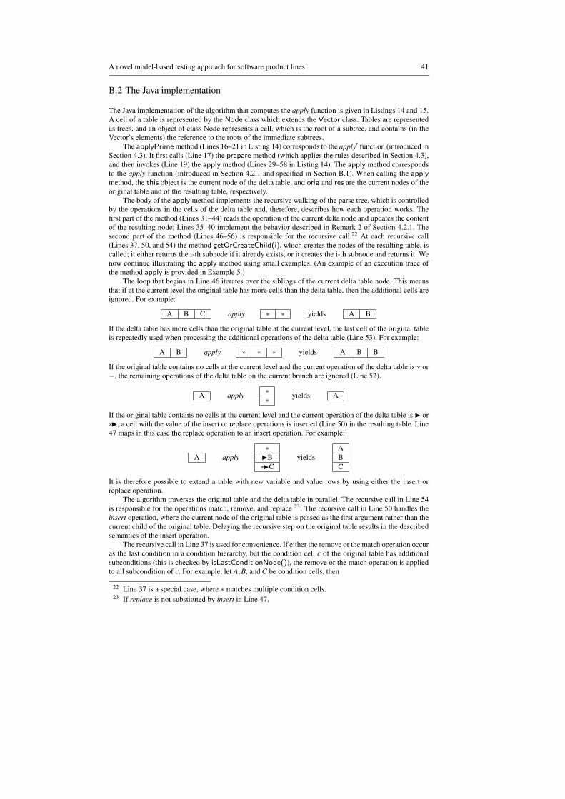
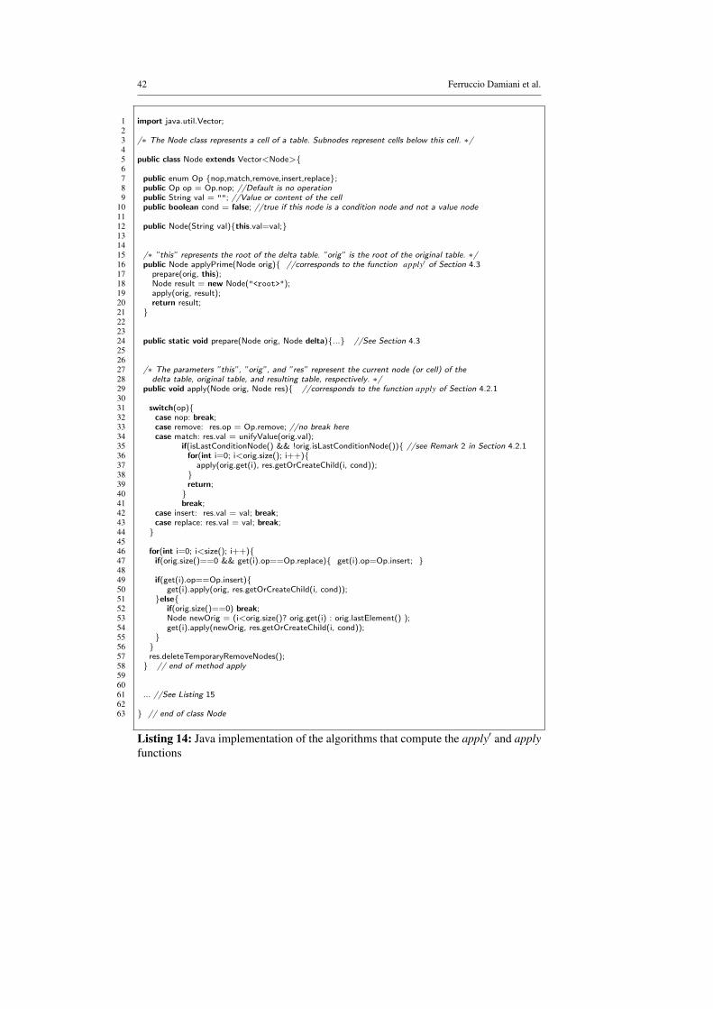
In this paper we address the problem of using the FineFit approach to supportthe development of correct SPLs. Writing for each product to be tested a FineFitspecification, a retrieve function, and a driver would be error prone and not cost-effective. Our idea is to express the specification of an SPL as a product line, whereeach product is a FineFit model (i.e., a set of tables) for the corresponding product(i.e., a Java program) of the specified SPL.
The main challenge addressed in this paper is to devise a means to concisely spec-ify the SPL being tested while retaining the readability of a FineFit specification ofa single system. To this aim, we consider delta-oriented programming (DOP) [36,7](see also [1], Section 6.6.1), a recently proposed flexible approach for implementingSPLs. DOP is an extension of feature-oriented programming (FOP) [5], a prominentapproach for developing SPLs (cf. [1], Section 6.1).1 DeltaJ [7,22,44] is the archety-pal language for delta-oriented programming of SPLs of Java programs.
As pointed out in [1], “much of the tremendous power of features is yet to be un-locked by making features explicit throughout the entire systems and software lifecy-cle”. In this paper we present DeltaFineFit, a novel model-based testing approach fordelta-oriented SPLs. DeltaFineFit integrates data refinement based testing into delta-oriented SPL development by ensuring that each product is generated together withits FineFit model and the suitable driver and retrieve functions.
1 A straightforward embedding of FOP into DOP is illustrated, e.g., in [38].
A novel model-based testing approach for software product lines 3
DeltaFineFit enables the fully automated testing of all the products of an SPL.When the number of products is too large, testing all the products is unfeasible. Thiscould be addressed by using, e.g., sample-based SPL testing techniques [21,20,27,23], where a subset of products—covering relevant combinations of features—is gen-erated and tested by applying single system testing techniques.
The main contribution of this paper is to introduce the delta table concept: anapproach for deriving a new table from an existing one, based on the difference (thedelta) between the tables. Delta tables are used to define a notion of “delta modulefor FineFit specifications” (i.e., a construct that describes how to modify the FineFitspecification of a product to obtain the FineFit specification of another product), thatwe call delta-table module. Delta tables are illustrated and evaluated (in terms of theirsupport to conciseness and readability of SPL specifications) by considering a smallSPL as a case study that is used as a running example throughout the paper.
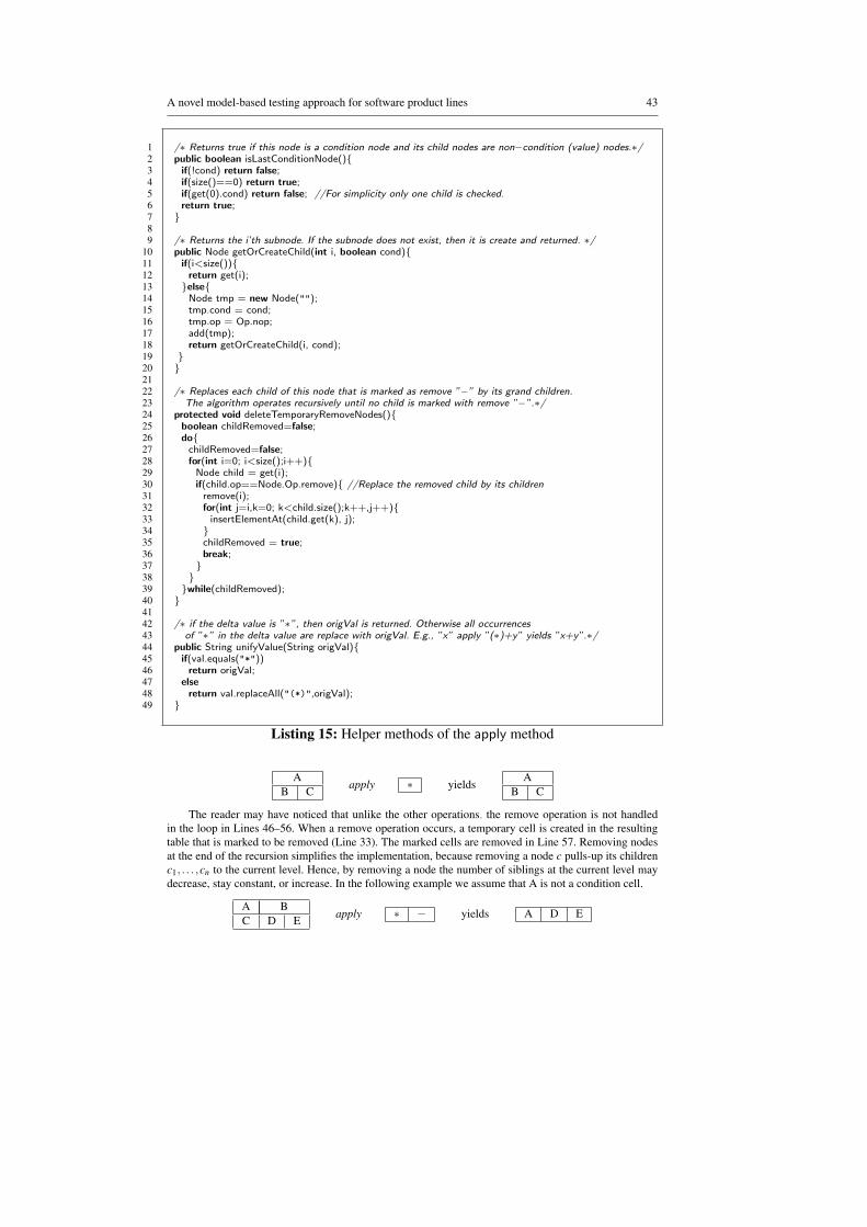
A prototypical implementation of DeltaTables, a tool that generates a FineFitspecification by applying a delta-table module to a FineFit specification, is avail-able at the DeltaFineFit home page [43]. All the tables presented in the paper that arethe result of delta-table application have been automatically generated. The DeltaFin-eFit tool chain (which will provide fully automated support to the integrated use ofDeltaTables, DeltaJ, and FineFit) is currently under development.
The remainder of the paper is organized as follows. Section 2 recalls the FineFitapproach for specifying and testing single Java programs. Section 3 recalls DOP andillustrates, by using DeltaJ, the SPL example that is used through the paper. Section 4introduces delta tables. Section 5 illustrates DeltaFineFit by means of the SPL intro-duced in Section 3. Section 6 evaluates the DeltaFineFit approach. Section 7 reviewssome related work. We conclude in Section 8 that also describes some future direc-tions. Appendix A elaborates on the structure and the semantics of the FineFit tables.Appendix B illustrates the algorithm that describes the semantics of delta tables.
A preliminary version of the material presented in this paper is briefly outlinedin [10]. Here we present a new and a more flexible notion of delta-tables, describeimplementation details, and provide detailed explanations and examples.
2 A recollection of data-refinement testing of Java programs with FineFit
The data refinement theory [34] captures the relationship between an abstract modeland its concrete implementation. The state spaces of the two levels of abstractionare related by a retrieve function which maps the concrete representation into theabstract one. When we use data refinement for testing, the abstract model becomes atest oracle and a source of test cases for the concrete program.
The FineFit [17,45] model-based (or model-driven) testing framework uses datarefinement to directly compare the state of the model (the specification) with the stateof the SUT. FineFit helps to understand the testing results and to trace the reason forany difference between the specification and the SUT (see [17]). To test a system,the user writes its specification as a collection of HTML2 tables (where cells contain
2 In practice the tables can be written using any tool that can export its output to HTML, for exampleMS Word. FineFit ignores anything that is not part of an HTML table.
4 Ferruccio Damiani et al.
Alloy expressions [19]). The specification of the SUT consists of tables for its basictypes (called atoms), for the states of the SUT, for its invariants, and one table foreach operation provided by the SUT. Each operation table defines an operation as apredicate on the system states immediately before and after the operation (similar tohow operations are specified in languages like Z [40]). FineFit uses these predicatesin two ways. First it uses the predicates to test the behavior of the SUT’s operations.For each operation X it applies the corresponding predicate to the SUT’s state, rightafter the SUT completes operation X . A false result indicates a discrepancy betweenthe expected and the actual behaviors. Second it uses the predicates to generate testcases by “solving” each predicate (a solution is an assignment of values that satisfythe predicate to the state variables and the inputs), and uses the solutions as testcases. These two capabilities are implemented with the help of Alloy’s3 Kodkod [41]relational model finder. We present an example in the rest of this section; for moredetails see [17].
The SUT’s retrieve function is a Java method that translates the concrete state (ofthe SUT) into an instance of the abstract state. The task of implementing the retrievefunction is delegated to the developer—who must know how the data structures im-plement the system’s specification. This makes the testing framework flexible andscalable, since the programmers can control the parts (i.e., select a subset) of the sys-tem to expose for the purpose of testing, even if the system is too large or complicatedfor automatic analysis.
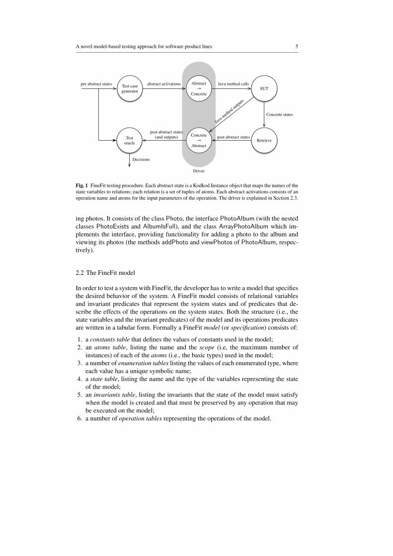
Figure 1 illustrates the testing process of a SUT when FineFit is used. Beforethe actual testing process is executed, FineFit checks the consistency of the model.Then FineFit begins the testing process by arbitrarily choosing an operation and inputavailable in the current state, applying the corresponding concrete operation to theSUT, and checking whether the new state corresponds to the operation’s specification.This process continues until either a discrepancy is found or until the user decides tostop the process. During testing, FineFit prints a trace that consists of the abstractsnapshots (states) and the operation calls of the SUT. When a problem is detected,the user can review the entire history that led to it.
In the following subsections we demonstrate data-refinement testing with FineFitby an example of a simple Java program implementing a photo album, that we callthe Base Album. We begin by describing in Section 2.1 the program we would liketo test. Then we describe in Section 2.2 the FineFit model that is used to test theprogram. Finally, in Section 2.3, we present the interfaces between FineFit and theprogram. These interfaces are used to retrieve the current program state for analysisin FineFit and to allow FineFit to apply operations on the program.
2.1 The Java program to be tested
Listing 1 shows the Java code implementing the Base Album. Informally, the BaseAlbum manages a sequence of photos and provides operations for adding and view-
3 Alloy is a general purpose modeling language (in the style of Z) for reasoning about relational struc-tures with first order logic. It has no direct concept of system states or operations, and it does not offer anytool for testing software.
A novel model-based testing approach for software product lines 5
Test case generator
Abstract →
Concrete
pre abstract states abstract activationsSUT
Java method calls
Concrete →
Abstract
Java m
ethod outputs
Retrieve
Concrete states
post abstract statesTest oracle
post abstract states (and outputs)
Driver
Decisions
Fig. 1 FineFit testing procedure. Each abstract state is a Kodkod Instance object that maps the names of thestate variables to relations; each relation is a set of tuples of atoms. Each abstract activations consists of anoperation name and atoms for the input parameters of the operation. The driver is explained in Section 2.3.
ing photos. It consists of the class Photo, the interface PhotoAlbum (with the nestedclasses PhotoExists and AlbumIsFull), and the class ArrayPhotoAlbum which im-plements the interface, providing functionality for adding a photo to the album andviewing its photos (the methods addPhoto and viewPhotos of PhotoAlbum, respec-tively).
2.2 The FineFit model
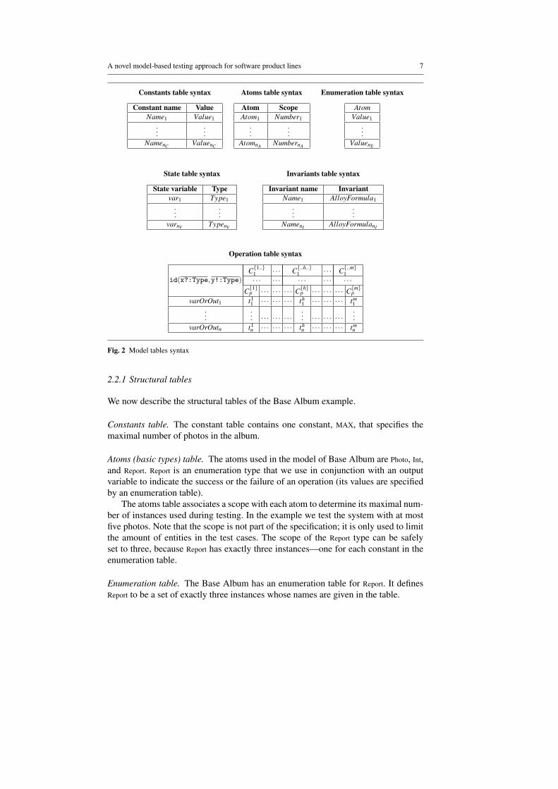
In order to test a system with FineFit, the developer has to write a model that specifiesthe desired behavior of the system. A FineFit model consists of relational variablesand invariant predicates that represent the system states and of predicates that de-scribe the effects of the operations on the system states. Both the structure (i.e., thestate variables and the invariant predicates) of the model and its operations predicatesare written in a tabular form. Formally a FineFit model (or specification) consists of:
1. a constants table that defines the values of constants used in the model;2. an atoms table, listing the name and the scope (i.e, the maximum number of
instances) of each of the atoms (i.e., the basic types) used in the model;3. a number of enumeration tables listing the values of each enumerated type, where
each value has a unique symbolic name;4. a state table, listing the name and the type of the variables representing the state
of the model;5. an invariants table, listing the invariants that the state of the model must satisfy
when the model is created and that must be preserved by any operation that maybe executed on the model;
6. a number of operation tables representing the operations of the model.
6 Ferruccio Damiani et al.
1 public class Photo {2 private String image; // represents the bitmap image3 public Photo(String theImage) {4 if(theImage == null) throw new IllegalArgumentException("NullImage");5 image = theImage;6 }7 public String getImage() { return image; }8 public String toString() { return image; }9 }
1 import java.util.Set;2 public interface PhotoAlbum {3 Photo addPhoto(String image);4 Set<Photo> viewPhotos();5 public class PhotoExists extends RuntimeException { }6 public class AlbumIsFull extends RuntimeException { }7 }
1 import java.util.Set;2 import java.util.HashSet;3 public class ArrayPhotoAlbum implements PhotoAlbum {4 private int size = 0;5 private Photo [] photoAt;6 public ArrayPhotoAlbum(int maxSize) {7 if(maxSize<1) throw new IllegalArgumentException("IllegalSize");8 photoAt = new Photo[maxSize];9 }
10 public boolean imageIsInAlbum(String image) {11 for (int i= 0; i < size; i++) {12 Photo p = photoAt[i];13 if (p.getImage().equals(image)) return true;14 }15 return false;16 }17 public Photo addPhoto(String image) {18 if(image == null) throw new IllegalArgumentException("NullImage");19 if(size == photoAt.length) throw new AlbumIsFull();20 if(imageIsInAlbum(image)) throw new PhotoExists();21 Photo new photo = new Photo(image);22 photoAt[size] = new photo;23 size = size + 1;24 return new photo;25 }26 public Set<Photo> viewPhotos() {27 Set<Photo> result = new HashSet<Photo>();28 for (int i= 0; i < size; i++) { result.add(photoAt[i]); }29 return result;30 }31 }
Listing 1: Java 1.5 code implementing the Base Album
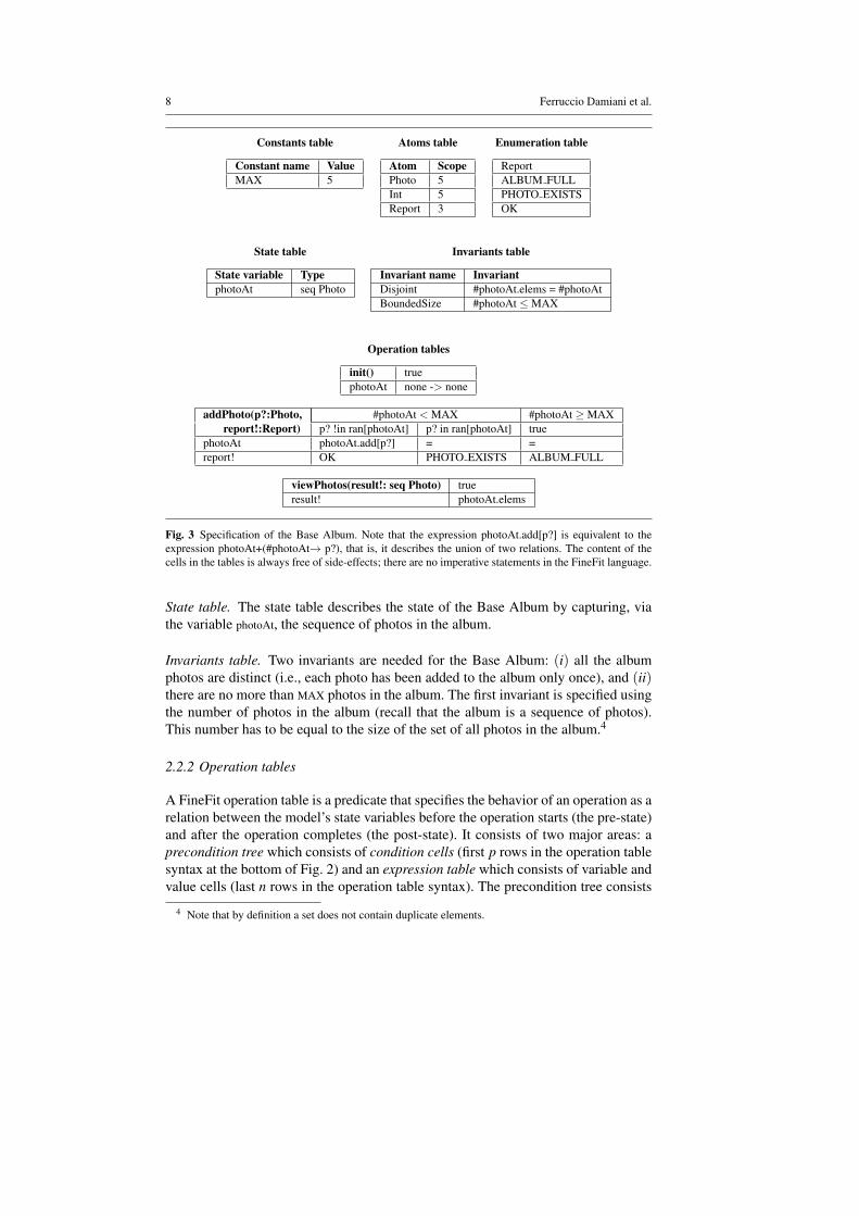
We name the first five kinds of tables structural tables (since they represent thestructure of the model). The syntax of the tables of the model is illustrated in Fig. 2.The model of the Base Album is given in Fig. 3. The expressions used in the tablesare written in Alloy [19], except that we use variables decorated with “?” and “!”to denote inputs and outputs, respectively. In most cases the expressions are self-explanatory; when needed we provide a short explanation.
A novel model-based testing approach for software product lines 7
We now describe the structural tables of the Base Album example.
Constants table. The constant table contains one constant, MAX, that specifies themaximal number of photos in the album.
Atoms (basic types) table. The atoms used in the model of Base Album are Photo, Int,and Report. Report is an enumeration type that we use in conjunction with an outputvariable to indicate the success or the failure of an operation (its values are specifiedby an enumeration table).
The atoms table associates a scope with each atom to determine its maximal num-ber of instances used during testing. In the example we test the system with at mostfive photos. Note that the scope is not part of the specification; it is only used to limitthe amount of entities in the test cases. The scope of the Report type can be safelyset to three, because Report has exactly three instances—one for each constant in theenumeration table.
Enumeration table. The Base Album has an enumeration table for Report. It definesReport to be a set of exactly three instances whose names are given in the table.
8 Ferruccio Damiani et al.
Constants table Atoms table Enumeration table
Constant name ValueMAX 5
Atom ScopePhoto 5Int 5Report 3
ReportALBUM FULLPHOTO EXISTSOK
State table Invariants table
State variable TypephotoAt seq Photo
Invariant name InvariantDisjoint #photoAt.elems = #photoAtBoundedSize #photoAt ≤MAX
Operation tables
init() truephotoAt none -> none
addPhoto(p?:Photo, #photoAt < MAX #photoAt ≥MAXreport!:Report) p? !in ran[photoAt] p? in ran[photoAt] true
photoAt photoAt.add[p?] = =report! OK PHOTO EXISTS ALBUM FULL
Fig. 3 Specification of the Base Album. Note that the expression photoAt.add[p?] is equivalent to theexpression photoAt+(#photoAt→ p?), that is, it describes the union of two relations. The content of thecells in the tables is always free of side-effects; there are no imperative statements in the FineFit language.
State table. The state table describes the state of the Base Album by capturing, viathe variable photoAt, the sequence of photos in the album.
Invariants table. Two invariants are needed for the Base Album: (i) all the albumphotos are distinct (i.e., each photo has been added to the album only once), and (ii)there are no more than MAX photos in the album. The first invariant is specified usingthe number of photos in the album (recall that the album is a sequence of photos).This number has to be equal to the size of the set of all photos in the album.4
2.2.2 Operation tables
A FineFit operation table is a predicate that specifies the behavior of an operation as arelation between the model’s state variables before the operation starts (the pre-state)and after the operation completes (the post-state). It consists of two major areas: aprecondition tree which consists of condition cells (first p rows in the operation tablesyntax at the bottom of Fig. 2) and an expression table which consists of variable andvalue cells (last n rows in the operation table syntax). The precondition tree consists
4 Note that by definition a set does not contain duplicate elements.
A novel model-based testing approach for software product lines 9
of predicates that determine which columns to use in the definition of the post-state.The expression table is a set of columns, where each column defines the values ofthe state variables in the post state (given their values in the pre-state) and the valuesof the output parameters. For example, the addPhoto operation of the Base Album (cf.Fig. 3) updates the state of the photoAt state variable and the report! output parameter(first column). This operation has three expression columns—columns two to four inthe table. The first expression column (the second column in the table) is for the casewhere the input photo p? (of type Photo) does not appear in the album and the albumis not full, then the photo is added to photoAt. The next expression column is forthe case where the input photo already appears in the non-full album (photoAt does notchange), and the last expression column is for the case where the album is full (photoAtdoes not change). The value of report! (of type Report) is OK only in the case that theaddPhoto operation indeed added a new photo to the album. Note that predicates thatappear on top of each other are conjoined, while predicates that appear side by siderepresent disjunction. If we consider the precondition part of an operation table (seethe operation table syntax, Fig. 2) as a matrix of p rows and m columns, then
– each of the predicates C{1}p ..C{m}p in row p occupies exactly one cell, and– each of the predicates C{1..}q ..C{..h..}q ..C{..m}q in row q (with 1≤ q≤ p) spans over
one or more consecutive cells (a predicate that spans over columns j..k is super-scripted by the set { j..k} of the indexes of those columns).
We provide further explanations about the structure and semantics of operation tablesin Appendix A.
In addition to addPhoto, the model of the Base Album provides the operations view-Photos and init. The operation viewPhotos uses elems to return (using result!) the set ofelements in a given sequence (in our case the photoAt sequence). Finally, the operationinit—which corresponds a class constructor in Java—defines the initial state of thealbum, demanding that there are no photos in the album.
The meaning of ‘=’ in a cell of the expression table part of an operation table(e.g., addPhoto in Fig. 3) is that the content of the state variable associated to the tablerow is left unchanged.
2.3 The retrieve function and the driver
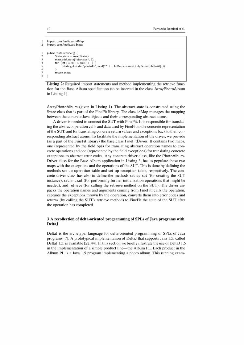
During the testing process, the SUT must provide FineFit with abstractions of itscurrent state, and FineFit must instruct the SUT to perform operations with specificinputs. The first task is supported by a retrieve function and the second by a driver.5
The retrieve function relates the concrete state of the SUT (Java code) to theabstract state of the specification. To provide a retrieve function the SUT must imple-ment a method that returns an abstract snapshot (a collection of named sets of tuples,one for each state variable) of its current state. For example, in our Base Albumapplication we have added the retrieve method illustrated in Listing 2 to the class
5 In the original paper about FineFit [17] we used the term fixture, which was borrowed from Fit [31],instead of driver. We think that driver is a more appropriate term.
1 public State retrieve() {2 State state = new State();3 state.add state("photoAt", 2);4 for (int i = 0; i < size; i++) {5 state.get state("photoAt").add("" + i, IdMap.instance().obj2atom(photoAt[i]));6 }7 return state;8 }
Listing 2: Required import statements and method implementing the retrieve func-tion for the Base Album specification (to be inserted in the class ArrayPhotoAlbumin Listing 1)
ArrayPhotoAlbum (given in Listing 1). The abstract state is constructed using theState class that is part of the FineFit library. The class IdMap manages the mappingbetween the concrete Java objects and their corresponding abstract atoms.
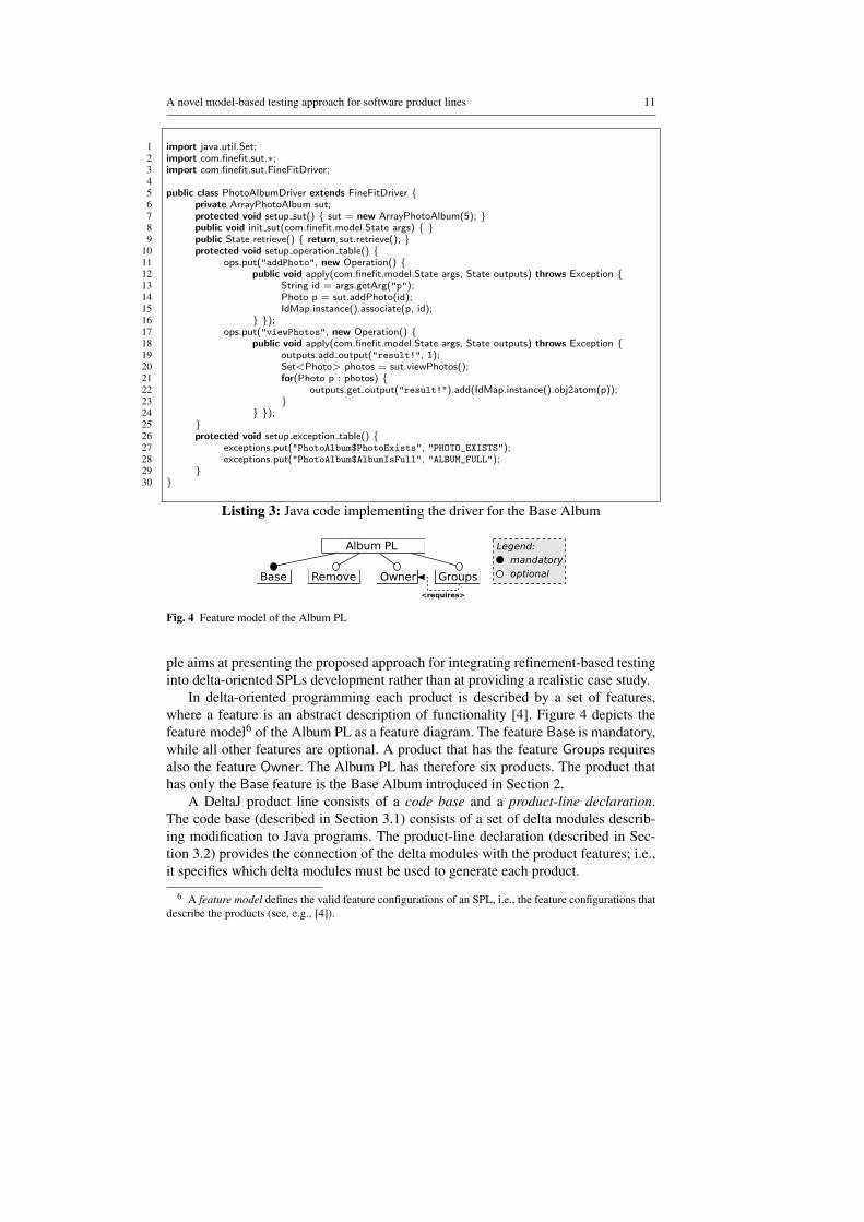
A driver is needed to connect the SUT with FineFit. It is responsible for translat-ing the abstract operation calls and data used by FineFit to the concrete representationof the SUT, and for translating concrete return values and exceptions back to their cor-responding abstract atoms. To facilitate the implementation of the driver, we provide(as a part of the FineFit library) the base class FineFitDriver. It contains two maps,one (represented by the field ops) for translating abstract operation names to con-crete operations and one (represented by the field exceptions) for translating concreteexceptions to abstract error codes. Any concrete driver class, like the PhotoAlbum-Driver class for the Base Album application in Listing 3, has to populate these twomaps with the exceptions and the operations of the SUT. This is done by defining themethods set up operation table and set up exception table, respectively. The con-crete driver class has also to define the methods set up sut (for creating the SUTinstance), set init sut (for performing further initialization operations that might beneeded), and retrieve (for calling the retrieve method on the SUT). The driver un-packs the operation names and arguments coming from FineFit, calls the operation,captures the exceptions thrown by the operation, converts them into error codes andreturns (by calling the SUT’s retrieve method) to FineFit the state of the SUT afterthe operation has completed.
3 A recollection of delta-oriented programming of SPLs of Java programs withDeltaJ
DeltaJ is the archetypal language for delta-oriented programming of SPLs of Javaprograms [7]. A prototypical implementation of DeltaJ that supports Java 1.5, calledDeltaJ 1.5, is available [22,44]. In this section we briefly illustrate the use of DeltaJ 1.5in the implementation of a simple product line—the Album PL. Each product in theAlbum PL is a Java 1.5 program implementing a photo album. This running exam-
A novel model-based testing approach for software product lines 11
1 import java.util.Set;2 import com.finefit.sut.∗;3 import com.finefit.sut.FineFitDriver;45 public class PhotoAlbumDriver extends FineFitDriver {6 private ArrayPhotoAlbum sut;7 protected void setup sut() { sut = new ArrayPhotoAlbum(5); }8 public void init sut(com.finefit.model.State args) { }9 public State retrieve() { return sut.retrieve(); }
10 protected void setup operation table() {11 ops.put("addPhoto", new Operation() {12 public void apply(com.finefit.model.State args, State outputs) throws Exception {13 String id = args.getArg("p");14 Photo p = sut.addPhoto(id);15 IdMap.instance().associate(p, id);16 } });17 ops.put("viewPhotos", new Operation() {18 public void apply(com.finefit.model.State args, State outputs) throws Exception {19 outputs.add output("result!", 1);20 Set<Photo> photos = sut.viewPhotos();21 for(Photo p : photos) {22 outputs.get output("result!").add(IdMap.instance().obj2atom(p));23 }24 } });25 }26 protected void setup exception table() {27 exceptions.put("PhotoAlbum$PhotoExists", "PHOTO_EXISTS");28 exceptions.put("PhotoAlbum$AlbumIsFull", "ALBUM_FULL");29 }30 }
Listing 3: Java code implementing the driver for the Base Album
Fig. 4 Feature model of the Album PL
ple aims at presenting the proposed approach for integrating refinement-based testinginto delta-oriented SPLs development rather than at providing a realistic case study.
In delta-oriented programming each product is described by a set of features,where a feature is an abstract description of functionality [4]. Figure 4 depicts thefeature model6 of the Album PL as a feature diagram. The feature Base is mandatory,while all other features are optional. A product that has the feature Groups requiresalso the feature Owner. The Album PL has therefore six products. The product thathas only the Base feature is the Base Album introduced in Section 2.
A DeltaJ product line consists of a code base and a product-line declaration.The code base (described in Section 3.1) consists of a set of delta modules describ-ing modification to Java programs. The product-line declaration (described in Sec-tion 3.2) provides the connection of the delta modules with the product features; i.e.,it specifies which delta modules must be used to generate each product.
6 A feature model defines the valid feature configurations of an SPL, i.e., the feature configurations thatdescribe the products (see, e.g., [4]).
12 Ferruccio Damiani et al.
3.1 DeltaJ delta modules
A DeltaJ delta module describes the changes in a given product (i.e., a Java pro-gram) that are needed to implement other products (i.e., other Java programs). Thealterations inside a delta module act both at the class/interface level by
– adding or removing a Java compilation unit, that is, an interface or a class togetherwith a package declaration and a list of import-statements, or
– modifying the package declarations, or– modifying the import-statements;
and at the class/interface structure level by
– modifying existing interfaces (i.e., changing the super interfaces and adding, re-moving or modifying method signatures or nested types), or
– modifying the internal structure of existing classes (i.e., changing the super classor the implemented interfaces and adding, removing or modifying constructors,fields, methods or nested types).
Modifying a method m of a class C means replacing the method body with a new one.The new body may contain the call original(· · ·), that is replaced in the generatedproduct by a call to a new method with a fresh name m’, which has the same type andbody as m before the modification. The new method m’ is added to the class C whenthe product is generated.7
3.2 DeltaJ product-line declaration
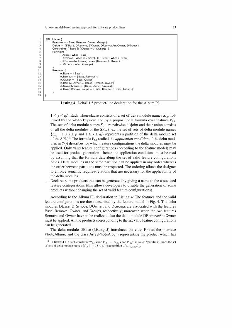
Listing 4 illustrates the declaration for the Album PL. The product line declaration:
– Lists the product features.– Lists the delta modules.– Describes the set of valid feature configurations by means of propositional con-
straints over the set of features (see, e.g., [4]). For each feature ϕ in the set {ϕ}of the product line features we introduce a propositional variable with the samename. A propositional formula P characterizes a set of feature configurationsΨ ⊆P({ϕ}) if and only if, for every feature configuration {ψ} ∈Ψ , the for-mula P is true when the variables in {ψ} are true and the variables in {ϕ}\{ψ}are false. The propositional formula in Listing 4 (Base & (Groups ⇒ Owner))represents the six valid feature configurations described by the feature diagram(Fig. 4).
– Describes the relation between delta modules and features by means of a totallyordered set of constraints called partitions. A partition consists of a set of when-clauses. When-clauses in the same partition are separated by a comma and theend of each partition is indicated by a semicolon. Consider p≥ 1 partitions, suchthat the i-th partition contains qi ≥ 1 delta clauses Si, j when Pi, j (1 ≤ i ≤ p and
7 This mechanism is similar to the Super(...) call of FOP [5] and to the around advice and proceedmechanisms of aspect-oriented programming (AOP)—see, e.g., [37,7] for a comparison between DOPand AOP.
A novel model-based testing approach for software product lines 13
1 SPL Album {2 Features = {Base, Remove, Owner, Groups}3 Deltas = {DBase, DRemove, DOwner, DRemoveAndOwner, DGroups}4 Constraints { Base & (Groups => Owner); }5 Partitions {6 {DBase} when (Base);7 {DRemove} when (Remove), {DOwner} when (Owner);8 {DRemoveAndOwner} when (Remove & Owner);9 {DGroups} when (Groups);
10 }11 Products {12 A Base = {Base};13 A Remove = {Base, Remove};14 A Owner = {Base, Owner};15 A RemoveOwner = {Base, Remove, Owner};16 A OwnerGroups = {Base, Owner, Groups};17 A OwnerRemoveGroups = {Base, Remove, Owner, Groups};18 }19 }
Listing 4: DeltaJ 1.5 product-line declaration for the Album PL
1 ≤ j ≤ qi). Each when-clause consists of a set of delta module names Si, j, fol-lowed by the when keyword and by a propositional formula over features Pi, j.The sets of delta module names Si, j are pairwise disjoint and their union consistsof all the delta modules of the SPL (i.e., the set of sets of delta module names{Si, j | 1 ≤ i ≤ p and 1 ≤ j ≤ qi} represents a partition of the delta module setof the SPL).8 The formula Pi, j (called the application condition of the delta mod-ules in Si, j) describes for which feature configurations the delta modules must beapplied. Only valid feature configurations (according to the feature model) maybe used for product generation—hence the application conditions must be readby assuming that the formula describing the set of valid feature configurationsholds. Delta modules in the same partition can be applied in any order whereasthe order between partitions must be respected. The ordering allows the designerto enforce semantic requires-relations that are necessary for the applicability ofthe delta modules.
– Declares some products that can be generated by giving a name to the associatedfeature configurations (this allows developers to disable the generation of someproducts without changing the set of valid feature configurations).
According to the Album PL declaration in Listing 4: The features and the validfeature configurations are those described by the feature model in Fig. 4. The deltamodules DBase, DRemove, DOwner, and DGroups are associated with the featuresBase, Remove, Owner, and Groups, respectively; moreover, when the two featuresRemove and Owner have to be realized, also the delta module DRemoveAndOwnermust be applied. All the products corresponding to the six valid feature configurationscan be generated.
The delta module DBase (Listing 5) introduces the class Photo, the interfacePhotoAlbum, and the class ArrayPhotoAlbum representing the product which has
8 In DELTAJ 1.5 each constraint “Si,1 when Pi,1, . . . , Si,qi when Pi,qi ;” is called “partition”, since the setof sets of delta module names {Si, j | 1≤ j ≤ qi} is a partition of ∪1≤ j≤qi Si, j .
14 Ferruccio Damiani et al.
1 delta DBase {2 adds { package it.unito.Album; /∗ Same as in Listing 1 (top) ∗/ }3 adds { package it.unito.Album; /∗ Same as in Listing 1 (middle)∗/ }4 adds { package it.unito.Album; /∗ Same as in Listing 1 (bottom)∗/ }5 }
Listing 5: Code base of the Album PL: delta module DBase
1 delta DRemove {23 modifies it.unito.Album.PhotoAlbum {4 adds public void removePhoto(int location);5 }67 modifies it.unito.Album.ArrayPhotoAlbum {8 adds public void removePhoto(int location) {9 if ((location < 0) || (size <= location))
10 modifies it.unito.Album.Photo {11 ... /∗Adds a field (group) and two methods (getGroup and setGroup) ∗/12 }1314 modifies it.unito.Album.PhotoAlbum {15 adds public User updateUser(String name, String password);16 adds public Group updateGroup(String name, Set<String> memberNames);17 adds public void removeUser(String name);18 adds public void removeGroup(String name);19 adds public void updatePhotoGroup(int location, String groupName);20 adds nested { public class MissingUser extends RuntimeException {} }21 adds nested { public class MissingUsers extends RuntimeException {} }22 adds nested { public class MissingGroup extends RuntimeException {} }23 adds nested { public class RemoveOwnerGroup extends RuntimeException {} }24 adds nested { public class RemoveOwner extends RuntimeException {} }25 }2627 modifies it.unito.Album.ArrayPhotoAlbum {28 ... /∗ Adds fields, modifies constructor, modifies methods, adds methods ∗/29 }3031 }
Listing 9: Code base of the Album PL: delta module DGroups
only the Base feature (cf. Section 2.1). The delta module DRemove (Listing 6) in-troduces the Remove feature which enables to remove a photo from the album. Thedelta module DOwner (Listing 7) introduces the Owner feature which protects thephoto album by enabling only the owner (who has to login) to modify the album. Thedelta module DRemoveAndOwner (Listing 8) introduces the code needed to handlethe combination of the optional features DRemove and DOwner. The delta moduleDGroups (Listing 9) introduces a further level of protection by requiring the ownerto create users and to associate to each photo the group of users that can view it. Thecomplete code of the delta modules of the Album PL is available at the DeltaFineFithome page [43].
16 Ferruccio Damiani et al.
3.3 DeltaJ generation of the products
A product is valid if it corresponds to a valid feature configuration. The productgeneration mapping is the mapping that associates each valid feature configurationto the corresponding product (i.e., the Java program obtained by applying the deltamodules with a satisfied when-clause to the empty program). This mapping may bepartial (since a non-applicable delta module may be encountered during product gen-eration, resulting in an undefined product) and ambiguous (since, for a given featureconsideration, two different orders of the delta-modules that are compatible with theorder of the partitions may generate two different products).
A delta module is applicable to a Java program if suitable syntactic conditions aresatisfied. E.g.:
– each class or interface to be added does not exists;– each class or interface to be removed or modified exists;– for every interface to be modified: each method to be added does not exist, each
method to be removed exists; and– for every class to be modified: each method or field to be added does not exist,
each method or field to be removed exists, and each method to be modified existsand has the same signature as in the method-modify operation.
A suitable type system could guarantee that if a DeltaJ product line is well-typed,then its product generation mapping is total and unambiguous and all its products arewell-typed Java programs. Such a type system has been formalized for the minimalcore calculus IMPERATIVE FEATHERWEIGHT DELTA JAVA (IF∆J) [7]. However, itis not yet implemented in DeltaJ 1.5 [22,44], where the products are generated byconsidering delta modules in the order in which they occur in the product line dec-laration,9 and most type errors in the products are detected only when the product isgenerated.
3.4 Delta-oriented SPL development
Delta-oriented programming is a transformational approach for the development ofSPLs [39]. For instance, it supports developing an SPL by starting from at least onecomplete product, called the core product, and writing program transformations (thedelta modules) that specify changes to be applied to the core product in order toimplement other products. In the following we use the phrase core delta module torefer to a delta module that when applied to the empty product generates the code ofa complete product.
The main advantage of transformational approaches over compositional ones (suchas, e.g., FOP [5,3,14,2]) is that when developing an SPL starting from a set of coreproducts, the latter approaches require to begin from simple products (implement-ing minimal sets of features) to be extended in order to implement the other prod-ucts. Instead, DOP supports also developing an SPL starting from complex products(implementing arbitrary large sets of features) and transforming them into simpler
9 Thus ruling out ambiguity.
A novel model-based testing approach for software product lines 17
1 SPL Album {2 Features = ... /∗ Same as in Listing 4 ∗/3 Deltas = ... /∗ Same as in Listing 4 ∗/4 Constraints {... /∗ Same as in Listing 4 ∗/ }5 Partitions {6 {Dall} when (Base);7 {DnoGroups} when (!Groups);8 {DnoOwner} when (!Owner);9 {DnoRemove} when (!Remove);
10 }11 Products { ... /∗ Same as in Listing 4 ∗/ }12 }
Listing 10: DeltaJ 1.5 product-line declaration for the complex-core implementationof the Album PL
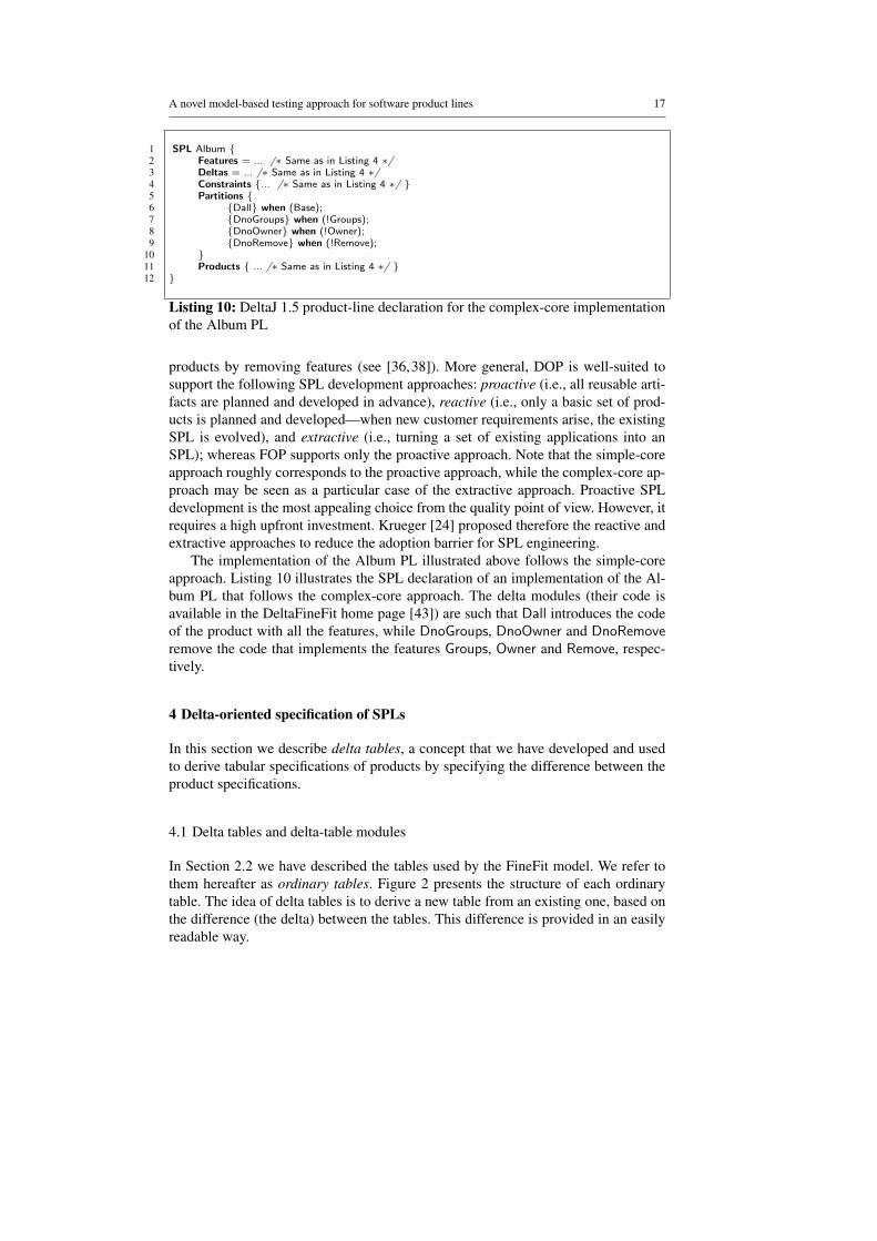
products by removing features (see [36,38]). More general, DOP is well-suited tosupport the following SPL development approaches: proactive (i.e., all reusable arti-facts are planned and developed in advance), reactive (i.e., only a basic set of prod-ucts is planned and developed—when new customer requirements arise, the existingSPL is evolved), and extractive (i.e., turning a set of existing applications into anSPL); whereas FOP supports only the proactive approach. Note that the simple-coreapproach roughly corresponds to the proactive approach, while the complex-core ap-proach may be seen as a particular case of the extractive approach. Proactive SPLdevelopment is the most appealing choice from the quality point of view. However, itrequires a high upfront investment. Krueger [24] proposed therefore the reactive andextractive approaches to reduce the adoption barrier for SPL engineering.
The implementation of the Album PL illustrated above follows the simple-coreapproach. Listing 10 illustrates the SPL declaration of an implementation of the Al-bum PL that follows the complex-core approach. The delta modules (their code isavailable in the DeltaFineFit home page [43]) are such that Dall introduces the codeof the product with all the features, while DnoGroups, DnoOwner and DnoRemoveremove the code that implements the features Groups, Owner and Remove, respec-tively.
4 Delta-oriented specification of SPLs
In this section we describe delta tables, a concept that we have developed and usedto derive tabular specifications of products by specifying the difference between theproduct specifications.
4.1 Delta tables and delta-table modules
In Section 2.2 we have described the tables used by the FineFit model. We refer tothem hereafter as ordinary tables. Figure 2 presents the structure of each ordinarytable. The idea of delta tables is to derive a new table from an existing one, based onthe difference (the delta) between the tables. This difference is provided in an easilyreadable way.
18 Ferruccio Damiani et al.
A delta table is recognized by its name (the upper-left cell), which is precededwith the ∆ symbol. Delta tables have the same structure as the ordinary tables, yettheir cells may contain delta operators (namely, match “∗”, remove “−”, insert “I”,and replace “∗I”). Let us denote the set of ordinary tables by TO and the set ofdelta tables by T∆ . A delta table t∆ can be applied to an ordinary table to, writ-ten as apply(to, t∆ ), resulting in a new ordinary table. That is, apply is a functionapply : TO×T∆ → TO ∪ ε , where ε denotes an empty (non-existent) table in thecase that the table is removed by the application. Following is an example of a deltatable application which yields a resulting table (to be explained later). We use theinfix notation: TO apply T∆ .
f(x) x < 0 x≥ 0y x xz 1 0
apply∆ f(x) x < 0 x≥ 0
y ∗I-x ∗− − −
yields
f(x) x < 0 x≥ 0y -x x
A delta-table module (DTM) is a set of delta and non-delta tables. Delta tablemodules specify the changes to the FineFit specification of a product that are neededto obtain the specification of another product (i.e., another set of tables). For this weintroduce the function Apply : P(TO)×P((TO∪T∆ ))→P(TO), where P(TO) andP(T∆ ) denote sets of tables.
To define the Apply function we must distinguish between a table and its name,since when overriding a table a with a table b the tables may be different, i.e. a 6= b,yet they must share the same name, e.g., specify the same operation. Let t denote thename of table t and T denote the set of all table names of the set of tables T . A deltatable module B ∈P((TO∪T∆ )) is applied to a FineFit specification A ∈P(TO) asfollows:
Apply(A,B) =⋃
a∈A,b∈B
{a} if a /∈ B{b} if b ∈ TO{apply(a,b)} if b ∈ T∆ ,∆ a = b and apply(a,b) 6= ε
The three different cases are: (case 1) tables in original table set that are not presentin the DTM are copied to the resulting set of tables; (case 2)10 ordinary tables of theDTM are copied to the resulting table (and may overwrite tables from the original setA); and (case 3) if a table is marked with the ∆ symbol, then it is a delta table and it isapplied to the corresponding table in the original set. When apply(a,b) returns ε , a iseffectively removed. Note that multiple conditions may be satisfied simultaneously;in this case all tables whose conditions are satisfied are included.
The first version of delta tables, as proposed in [10], is capable of describing ina concise and an intuitive way the modification of value and variable cells and therefinement of condition cells. The latter means that subconditions can be introducedbelow existing condition cells of a table. We realized, however, that this conditionrefinement is not sufficient for handling all modifications that are necessary in prac-tice, as it is often required to change the condition hierarchy in a more complex way.
10 Note that tables satisfying this case do not satisfy case 1.
A novel model-based testing approach for software product lines 19
foo A BC D E F
x 1 2 3 4y i ii iii iv
<root>
foo
x
y
A
C
1
i
D
2
ii
B
E
3
iii
F
4
iv
Fig. 5 Table foo and its tree structure representation (used for explanations)
We have investigated several syntactic notations; for example, dividing the conditioncells into sections with different semantics of applications. Those notations, however,either have been complex or their application process was hard to understand.
The challenge of defining transformations on Parnas tables results from the factthat Parnas tables have both a tabular and a hierarchical structure. When definingoperations, we have to decide whether the tables should be treated as matrices oras trees. We found that embedding a matrix in a tree is easier than the other wayaround, and it allows us to define basic operations that are applicable to all kindsof tables and to all kinds of cells. In particular, these operations allow a concisetreatment of hierarchical conditional cells which is the most difficult feature to design.These operations are defined by the apply function that is introduced in Section 4.2.To handle also the matrix structure of the tables in a concise way and to providealso abbreviations and convenience rules for the user, we define another function–“prepare”, which is described in Section 4.3. A strength of the approach is that it hasone core algorithm that is relatively small and is recursively and uniformly appliedon all kinds of cells of the table. Furthermore, the same algorithm is applied to allkinds of tables in our framework.
4.2 Hierarchical representation of tables and operations of delta tables
Delta tables have the same syntax as the tables shown in Fig. 2. However, theircells may contain special symbols representing operations that are executed by theapply function. The operations and their corresponding symbols are: match “∗”, re-move “−”, insert “I”, and replace “∗I”. In order to deal with the condition hierarchyof operation tables, the apply function treats tables as ordered trees rather than as ma-trices, and traverses them recursively from top to bottom. Consider, for example, thetable foo and its encoding as a tree (Fig. 5). The columns of the table are the branchesof the tree. A table cell c1 which is located directly below cell c0 is a child of c0 in thetree representation. If c0 spans several cells, e.g., c1, . . . ,ck, those cells are childrenof c0. The order of siblings must be the same as in the table. Implicitly there also ispresent a <root> cell, whose children are the top level cells of the table. Note thateach cell represents a tree, namely the subtree which has the cell as its root. Hence,the entire tree is represented by the <root> cell.
20 Ferruccio Damiani et al.
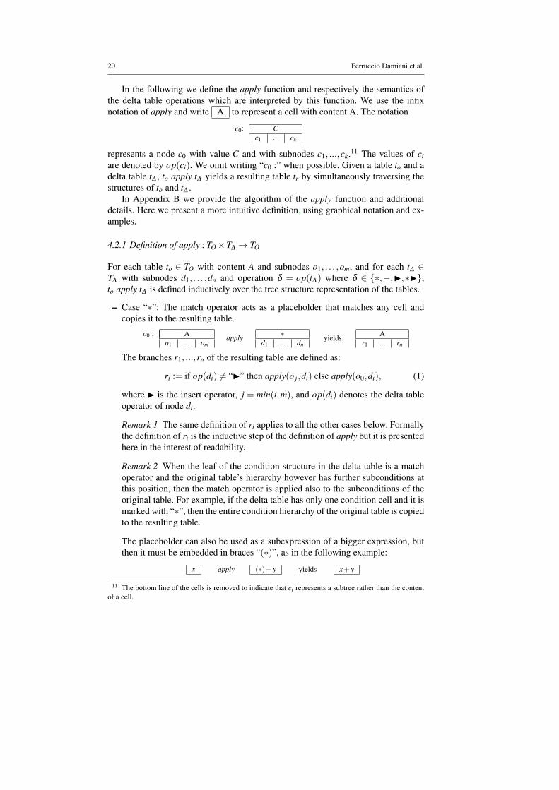
In the following we define the apply function and respectively the semantics ofthe delta table operations which are interpreted by this function. We use the infixnotation of apply and write A to represent a cell with content A. The notation
c0: Cc1 ... ck
represents a node c0 with value C and with subnodes c1, ...,ck.11 The values of ciare denoted by op(ci). We omit writing “c0 :” when possible. Given a table to and adelta table t∆ , to apply t∆ yields a resulting table tr by simultaneously traversing thestructures of to and t∆ .
In Appendix B we provide the algorithm of the apply function and additionaldetails. Here we present a more intuitive definition, using graphical notation and ex-amples.
4.2.1 Definition of apply : TO×T∆ → TO
For each table to ∈ TO with content A and subnodes o1, . . . ,om, and for each t∆ ∈T∆ with subnodes d1, . . . ,dn and operation δ = op(t∆ ) where δ ∈ {∗,−,I,∗I},to apply t∆ is defined inductively over the tree structure representation of the tables.
– Case “∗”: The match operator acts as a placeholder that matches any cell andcopies it to the resulting table.
o0 : Ao1 ... om
apply∗
d1 ... dnyields
Ar1 ... rn
The branches r1, ...,rn of the resulting table are defined as:
ri := if op(di) 6= “I” then apply(o j,di) else apply(o0,di), (1)
where I is the insert operator, j = min(i,m), and op(di) denotes the delta tableoperator of node di.
Remark 1 The same definition of ri applies to all the other cases below. Formallythe definition of ri is the inductive step of the definition of apply but it is presentedhere in the interest of readability.
Remark 2 When the leaf of the condition structure in the delta table is a matchoperator and the original table’s hierarchy however has further subconditions atthis position, then the match operator is applied also to the subconditions of theoriginal table. For example, if the delta table has only one condition cell and it ismarked with “∗”, then the entire condition hierarchy of the original table is copiedto the resulting table.
The placeholder can also be used as a subexpression of a bigger expression, butthen it must be embedded in braces “(∗)”, as in the following example:
x apply (∗)+ y yields x+ y
11 The bottom line of the cells is removed to indicate that ci represents a subtree rather than the contentof a cell.
A novel model-based testing approach for software product lines 21
– Case “−”: The remove operator matches any cell content A and removes the cellfrom the resulting table.
Ao1 ... om
apply−
d1 ... dnyields r1 ... rn
The following example combines operations. The first operation removes a cell(i.e., it is not copied to the resulting table) whereas the second copies the cell intothe resulting table.
AD
apply−∗ yields D
– Case “I”: The insert operator inserts a cell cins at the position of the current cellci of the original table. The apply function proceeds on subsequent cells as ifci and all its siblings, c1, . . . ,ci, . . . ,cn, are children of cins. The insert operationis defined partially by the following schema and partially by the recursive stepdescribed above (Equation 1).
Ao1 ... om
applyII
d1 ... dnyields
Ir1 ... rn
The following example presents the case where cins has a subsequent cell:
A applyII∗ yields
IA
We now demonstrate the case where cins has several subsequent cells:
A1 . . . An applyII
∗ . . . ∗ yieldsI
A1 . . . An
Multiple insert operations can be applied to the current cell of the original table.This results in several subbranches such that the children c1, . . . ,cn of c0 occur oneach subbranch. This is the desired behavior for refining conditions. For example,
AC D
apply∗
II IJ∗ ∗ ∗ ∗
yieldsA
I JC D C D
– Case “∗I”: The replace operation replaces the current cell of the original tablewith the cell of the delta table. This operation can be simulated by a combina-tion of remove and insert operations; introducing it, however, greatly improvesreadability. For example,
Ao1 ... om
apply∗IX
d1 ... dnyields
Xr1 ... rn
If the replace operation cannot be applied because the original table does notcontain a cell at the current position (e.g., it is at the end of the branch), theoperation is changed to an insert operation.
Let us demonstrate the application of a delta table that consists of one columnand contains all the described operators. The apply function simultaneously traversesboth the original and the delta tables from top to bottom and applies the delta tableoperators. For convenience, we write the recursion step numbers of the apply functionleft to the cells.
22 Ferruccio Damiani et al.
1: A2,3: C
4: 15: i6: w
apply
1: *2: II3: ∗4: ∗ID5: −6: ∗
yields
1: A2: I3: C4: D6: w
Here we show the application of a hierarchical delta table with several columns(branches):
AC D1 2i ii
apply
∗II IJ− ∗ ∗ −− ∗ ∗IX −− ∗ ∗IY −
yields
AI JD C2 Xii Y
Note that the apply function treats columns independently and does not preventvertical misalignment. Delta tables have to be written in such way that the desiredoutcome is generated, e.g. Parnas tables. The next section describes techniques thathelp writing delta tables.
4.3 Preprocessing rules
The apply function defined in the previous section takes care of the hierarchical natureof Parnas tables and provides a simple core transformation that is uniformly appliedto all cells. Here we introduce the prepare function, which takes care of the tabular12
nature of Parnas tables and defines a set of rules that simplify writing and reading ofdelta tables. The prepare function acts as a transformation layer on top of the applyfunction, i.e., it compiles a delta table with abbreviations and higher-level constructsinto a delta table that uses only the basic operations.
The preprocessing rules are defined by the function prepare : TO × T∆ → T∆
which takes as parameters an ordinary table and a delta table and returns a resultingdelta table. The resulting delta table is used as input to the apply function, as hasbeen defined in the previous section. The function apply′ : TO× T∆ → TO ∪ ε is thecomposition of the apply : TO× T∆ → TO∪ε and the prepare functions and is definedas:
apply′(to, t∆ ) = apply(to,prepare(to, t∆ )) (2)
for all to ∈ TO and t∆ ∈ T∆ . The function Apply′ : P(TO)×P((TO∪T∆ ))→P(TO)which applies a delta-table module on a set of ordinary tables is similar to the functionApply that is described in Section 4.1, but uses the function apply′ rather than apply.
In the following we informally describe the prepare function with a set of rulesthat must be applied in the given order. Some of the rules do not depend on a particularordinary table, and in this case we omit the ordinary table (i.e., we omit writing thefirst argument).
12 Unlike the apply function, the prepare function is aware of the row-alignment of cells in a table andprovides special treatment for different kinds of cells.
A novel model-based testing approach for software product lines 23
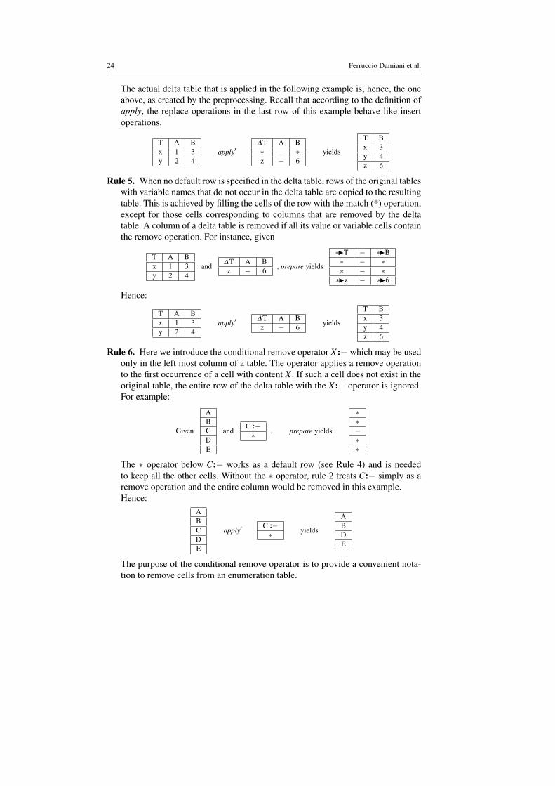
Rule 1. When the delta table contains a cell with no associated operation, ∗I is thedefault operation. Thus in principle the user does not have to use the ∗I symbol.However, the user should write ∗I explicitly when a cell’s content is changed toindicate that it is not just overwritten with the same content.Recall that ∗I can behave like an insert operation (from the definition of applyin Section 4.2.1). Hence, depending on the position of ∗I and its content it canreplace a cell, keep a cell (by replacing it with the same content), or insert a cell.The leading ∆ symbol is removed from the name of the delta table to match thename with the original table.
Rule 2. If all cells below a condition cell or a name cell c contain the remove opera-tion, c is removed as well. For example:13
∆T AB C
D − F Gx − 2 − −y − ii − −
prepare yields
∗IT ∗IA∗IB −
− − − −∗Ix − ∗I2 − −∗Iy − ∗Iii − −
The first rule is applied here and is responsible for adding the ∗I operations.The cells A and B are not removed because cells exist below them which are notremoved, namely 2 and ii.This rule enables the user to remove a column of value cells and the correspondingconditions, without having to write “−” in the condition cells. This makes it easierto see which condition is removed. Furthermore, this rule enables to remove anentire table T from the DTM by writing:
∆T−
In order to remove all cells of the table except for the name cell, the user maywrite ∆T .
Rule 3. A variable cell may contain a set of variables. These are expanded by thepreprocessing step into a set of rows, one for each variable. For instance:
Given∆T A B{x,y} 1 3
, prepare yields∗I T ∗I A ∗I B∗I x ∗I 1 ∗I 3∗I y ∗I 1 ∗I 3
Rule 4. The user may write ∗ in a variable cell in order to refer to all variables ofthe original table that are not explicitly mentioned in the delta table. A row thatcontains the ∗ operator in its variable cell is called a default row. Only one defaultrow may be specified. A default row is added for each variable not mentioned inthe variable cells of the delta table.14 For instance, given
T A Bx 1 3y 2 4
and∆T A B∗ − ∗z − 6
prepare yields
∗IT − ∗IB∗ − ∗∗ − ∗∗Iz − ∗I6
13 Recall that the row span of the name cell defines that the first three rows of the example are conditionrows and the other rows contain variable and value cells.
14 This includes variables checked by the conditional operator.
24 Ferruccio Damiani et al.
The actual delta table that is applied in the following example is, hence, the oneabove, as created by the preprocessing. Recall that according to the definition ofapply, the replace operations in the last row of this example behave like insertoperations.
T A Bx 1 3y 2 4
apply′∆T A B∗ − ∗z − 6
yields
T Bx 3y 4z 6
Rule 5. When no default row is specified in the delta table, rows of the original tableswith variable names that do not occur in the delta table are copied to the resultingtable. This is achieved by filling the cells of the row with the match (*) operation,except for those cells corresponding to columns that are removed by the deltatable. A column of a delta table is removed if all its value or variable cells containthe remove operation. For instance, given
T A Bx 1 3y 2 4
and∆T A Bz − 6
, prepare yields
∗IT − ∗IB∗ − ∗∗ − ∗∗Iz − ∗I6
Hence:
T A Bx 1 3y 2 4
apply′∆T A Bz − 6
yields
T Bx 3y 4z 6
Rule 6. Here we introduce the conditional remove operator X:− which may be usedonly in the left most column of a table. The operator applies a remove operationto the first occurrence of a cell with content X . If such a cell does not exist in theoriginal table, the entire row of the delta table with the X:− operator is ignored.For example:
Given
ABCDE
andC :−∗ , prepare yields
∗∗−∗∗
The ∗ operator below C:− works as a default row (see Rule 4) and is neededto keep all the other cells. Without the ∗ operator, rule 2 treats C:− simply as aremove operation and the entire column would be removed in this example.Hence:
ABCDE
apply′C :−∗ yields
ABDE
The purpose of the conditional remove operator is to provide a convenient nota-tion to remove cells from an enumeration table.
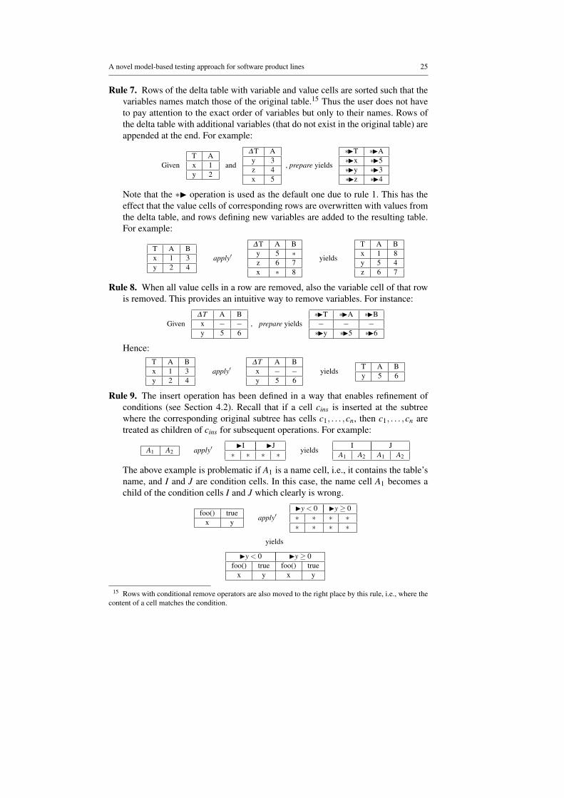
A novel model-based testing approach for software product lines 25
Rule 7. Rows of the delta table with variable and value cells are sorted such that thevariables names match those of the original table.15 Thus the user does not haveto pay attention to the exact order of variables but only to their names. Rows ofthe delta table with additional variables (that do not exist in the original table) areappended at the end. For example:
GivenT Ax 1y 2
and
∆T Ay 3z 4x 5
, prepare yields
∗IT ∗IA∗Ix ∗I5∗Iy ∗I3∗Iz ∗I4
Note that the ∗I operation is used as the default one due to rule 1. This has theeffect that the value cells of corresponding rows are overwritten with values fromthe delta table, and rows defining new variables are added to the resulting table.For example:
T A Bx 1 3y 2 4
apply′∆T A By 5 ∗z 6 7x ∗ 8
yields
T A Bx 1 8y 5 4z 6 7
Rule 8. When all value cells in a row are removed, also the variable cell of that rowis removed. This provides an intuitive way to remove variables. For instance:
Given∆T A Bx − −y 5 6
, prepare yields∗IT ∗IA ∗IB− − −∗Iy ∗I5 ∗I6
Hence:T A Bx 1 3y 2 4
apply′∆T A Bx − −y 5 6
yieldsT A By 5 6
Rule 9. The insert operation has been defined in a way that enables refinement ofconditions (see Section 4.2). Recall that if a cell cins is inserted at the subtreewhere the corresponding original subtree has cells c1, . . . ,cn, then c1, . . . ,cn aretreated as children of cins for subsequent operations. For example:
A1 A2 apply′II IJ∗ ∗ ∗ ∗ yields
I JA1 A2 A1 A2
The above example is problematic if A1 is a name cell, i.e., it contains the table’sname, and I and J are condition cells. In this case, the name cell A1 becomes achild of the condition cells I and J which clearly is wrong.
foo() truex y
apply′Iy < 0 Iy≥ 0∗ ∗ ∗ ∗∗ ∗ ∗ ∗
yields
Iy < 0 Iy≥ 0foo() true foo() true
x y x y
15 Rows with conditional remove operators are also moved to the right place by this rule, i.e., where thecontent of a cell matches the condition.
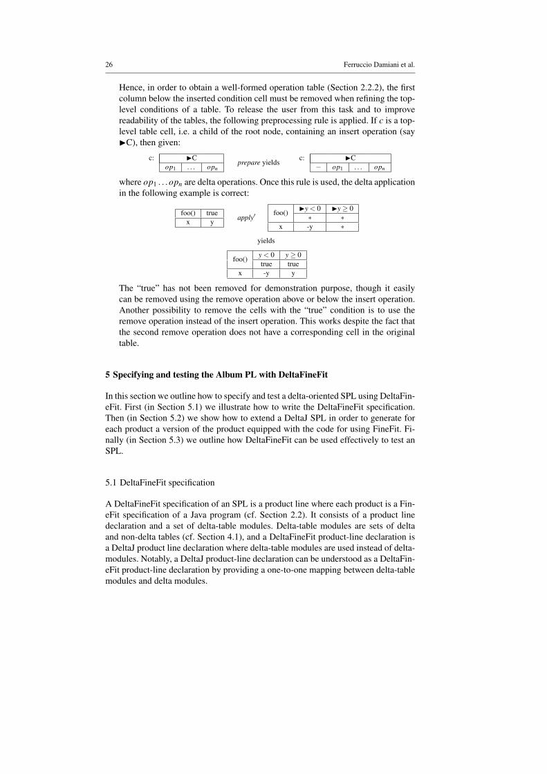
26 Ferruccio Damiani et al.
Hence, in order to obtain a well-formed operation table (Section 2.2.2), the firstcolumn below the inserted condition cell must be removed when refining the top-level conditions of a table. To release the user from this task and to improvereadability of the tables, the following preprocessing rule is applied. If c is a top-level table cell, i.e. a child of the root node, containing an insert operation (sayIC), then given:
c: ICop1 . . . opn
prepare yieldsc: IC
− op1 . . . opn
where op1 . . .opn are delta operations. Once this rule is used, the delta applicationin the following example is correct:
foo() truex y
apply′foo() Iy < 0 Iy≥ 0
∗ ∗x -y ∗
yields
foo() y < 0 y≥ 0true true
x -y y
The “true” has not been removed for demonstration purpose, though it easilycan be removed using the remove operation above or below the insert operation.Another possibility to remove the cells with the “true” condition is to use theremove operation instead of the insert operation. This works despite the fact thatthe second remove operation does not have a corresponding cell in the originaltable.
5 Specifying and testing the Album PL with DeltaFineFit
In this section we outline how to specify and test a delta-oriented SPL using DeltaFin-eFit. First (in Section 5.1) we illustrate how to write the DeltaFineFit specification.Then (in Section 5.2) we show how to extend a DeltaJ SPL in order to generate foreach product a version of the product equipped with the code for using FineFit. Fi-nally (in Section 5.3) we outline how DeltaFineFit can be used effectively to test anSPL.
5.1 DeltaFineFit specification
A DeltaFineFit specification of an SPL is a product line where each product is a Fin-eFit specification of a Java program (cf. Section 2.2). It consists of a product linedeclaration and a set of delta-table modules. Delta-table modules are sets of deltaand non-delta tables (cf. Section 4.1), and a DeltaFineFit product-line declaration isa DeltaJ product line declaration where delta-table modules are used instead of delta-modules. Notably, a DeltaJ product-line declaration can be understood as a DeltaFin-eFit product-line declaration by providing a one-to-one mapping between delta-tablemodules and delta modules.
A novel model-based testing approach for software product lines 27
The DeltaFineFit generation procedure is analogous to the DeltaJ 1.5 generationprocedure of a Java program (outlined in Section 3.3): given a valid feature configura-tion the DTMs with a satisfied when-clause are applied to the empty FineFit specifi-cation in the order in which they appear in the DeltaFineFit product-line declaration.This procedure describes a mapping that associates each valid feature configurationto the corresponding FineFit specification, and this mapping may be partial.
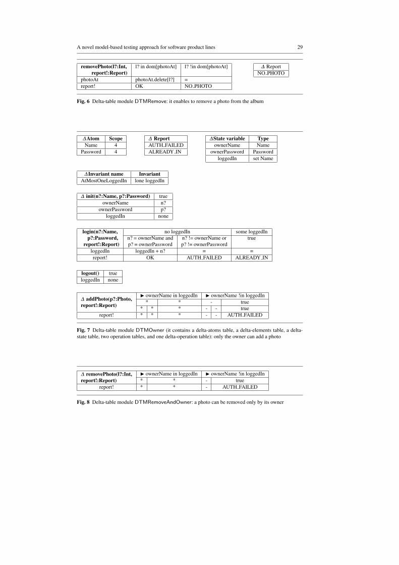
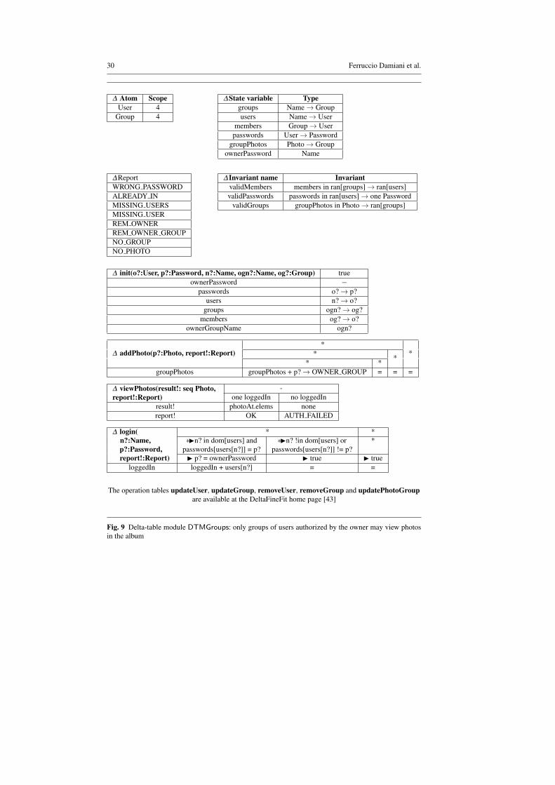
The tables describing the model of the Base Album (see Fig. 3) can be seen asthe DTMBase delta-table module that when applied to the empty abstract model pro-duces the model of the Base Album. The other DTMs of the Album PL specificationare listed in Figures 6, 7, 8, and 9. The delta-table module DTMRemove (Fig. 6)specifies the Remove feature which enables to remove a photo from the album. Thedelta-table module DTMOwner (Fig. 7) specifies the Owner feature which protectsthe photo album by enabling only the owner (who has to login) to modify the album.The DTMRemoveAndOwner delta-table module (Fig. 8) introduces the needed mod-ifications to specify the combination of the two optional features Remove and Owner.The delta-table module DTMGroups (Fig. 9) specifies a further level of protection byrequiring the owner to create users and to associate each photo with the group ofusers that can view it.
The simple-core implementation of the Album PL (Listing 4) can therefore beunderstood as the DeltaFineFit product-line declaration for the specification of theAlbum PL, modulo the mapping that associates the delta-table modules DTMBase,DTMRemove, DTMOwner, DTMRemoveAndOwner, and DTMOwner to the deltamodules DBase, DRemove, DOwner, DRemoveAndOwner, and DOwner, respec-tively.
The specification of the Album PL (Figures 6 – 9) uses the simple-core approach(cf. Section 3.4). The declaration of the complex-core DeltaJ 1.5 implementation ofthe Album PL given in Listing 10 can be used as a declaration of a complex-coreDeltaFineFit specification of the Album PL. This is achieved by associating to thedelta modules Dall, DnoGroups, DnoOwner, and DnoRemove the appropriate delta-table modules DTMall, DTMnoGroups, DTMnoOwner, and DnoRemove, respec-tively. The tables of the complex-core specification are available at the DeltaFineFithome page [43]. Note that the tables of the core DTM for the product with all features,DTMall, are the tables in the specification of the product with all features.
In the following examples we take a close look at some of the specification tablesfrom the figures.
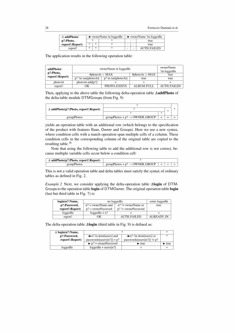
Example 1 This example shows the application of the ∆addPhoto delta-operationtable of the delta-table module DTMOwner to the operation table addPhoto of thebase product. The original operation table (from Fig. 3) is defined as:
addPhoto(p?:Photo, #photoAt < MAX #photoAt ≥MAXreport!:Report) p? !in ran[photoAt] p? in ran[photoAt] true
photoAt photoAt.add[p?] = =report! OK PHOTO EXISTS ALBUM FULL
The delta-operation table (at the bottom of Fig. 7) is defined as:
28 Ferruccio Damiani et al.
∆ addPhoto(p?:Photo,report!:Report)
I ownerName in loggedIn I ownerName !in loggedIn* * - true
* * * - - truereport! * * * - - AUTH FAILED
The application results in the following operation table:
addPhoto(p?:Photo,report!:Report)
ownerName in loggedIn ownerName!in loggedIn
#photoAt < MAX #photoAt ≥MAX truep? !in ran[photoAt] p? in ran[photoAt] true true
photoAt photoAt.add[p?] = = =report! OK PHOTO EXISTS ALBUM FULL AUTH FAILED
Then, applying to the above table the following delta-operation table ∆addPhoto ofthe delta-table module DTMGroups (from Fig. 9)
∆ addPhoto(p?:Photo, report!:Report)*
** ** *
groupPhotos groupPhotos + p?→ OWNER GROUP = = =
yields an operation table with an additional row (which belongs to the specificationof the product with features Base, Owner and Groups). Here we use a new syntax,where condition cells with a match operation span multiple cells of a column. Thesecondition cells in the corresponding column of the original table are copied to theresulting table.16
Note that using the following table to add the additional row is not correct, be-cause multiple variable cells occur below a condition cell:
This is not a valid operation table and delta tables must satisfy the syntax of ordinarytables as defined in Fig. 2.
Example 2 Next, we consider applying the delta-operation table ∆ login of DTM-Groups to the operation table login of DTMOwner. The original operation table login(last but third table in Fig. 7) is:
login(n?:Name, no loggedIn some loggedInp?:Password, n? = ownerName and n? != ownerName or truereport!:Report) p? = ownerPassword p? != ownerPassword
loggedIn loggedIn + n? = =report! OK AUTH FAILED ALREADY IN
The delta-operation table ∆ login (third table in Fig. 9) is defined as:
∆ login(n?:Name, * *p?:Password, ∗In? in dom[users] and ∗In? !in dom[users] or *report!:Report) passwords[users[n?]] = p? passwords[users[n?]] != p?
I p? = ownerPassword I true I trueloggedIn loggedIn + users[n?] = =
A novel model-based testing approach for software product lines 29
removePhoto(l?:Int, l? in dom[photoAt] l? !in dom[photoAt]report!:Report)
photoAt photoAt.delete[l?] =report! OK NO PHOTO
∆ ReportNO PHOTO
Fig. 6 Delta-table module DTMRemove: it enables to remove a photo from the album
∆Atom ScopeName 4
Password 4
∆ ReportAUTH FAILEDALREADY IN
∆State variable TypeownerName Name
ownerPassword PasswordloggedIn set Name
∆Invariant name InvariantAtMostOneLoggedIn lone loggedIn
∆ init(n?:Name, p?:Password) trueownerName n?
ownerPassword p?loggedIn none
login(n?:Name, no loggedIn some loggedInp?:Password, n? = ownerName and n? != ownerName or true
report!:Report) p? = ownerPassword p? != ownerPasswordloggedIn loggedIn + n? = =report! OK AUTH FAILED ALREADY IN
logout() trueloggedIn none
∆ addPhoto(p?:Photo,report!:Report)
I ownerName in loggedIn I ownerName !in loggedIn* * - true
* * * - - truereport! * * * - - AUTH FAILED
Fig. 7 Delta-table module DTMOwner (it contains a delta-atoms table, a delta-elements table, a delta-state table, two operation tables, and one delta-operation table): only the owner can add a photo
∆ removePhoto(l?:Int,report!:Report)
I ownerName in loggedIn I ownerName !in loggedIn* * - true
report! * * - AUTH FAILED
Fig. 8 Delta-table module DTMRemoveAndOwner: a photo can be removed only by its owner
30 Ferruccio Damiani et al.
∆ Atom ScopeUser 4
Group 4
∆State variable Typegroups Name→ Groupusers Name→ User
∆ login( * *n?:Name, ∗In? in dom[users] and ∗In? !in dom[users] or *p?:Password, passwords[users[n?]] = p? passwords[users[n?]] != p?report!:Report) I p? = ownerPassword I true I true
loggedIn loggedIn + users[n?] = =
The operation tables updateUser, updateGroup, removeUser, removeGroup and updatePhotoGroupare available at the DeltaFineFit home page [43]
Fig. 9 Delta-table module DTMGroups: only groups of users authorized by the owner may view photosin the album
A novel model-based testing approach for software product lines 31
1 SPL Album {2 Features = {Base, Remove, Owner, Groups, FineFit}3 Deltas = {DBase, DRemove, DOwner, DRemoveAndOwner, DGroups,4 DBaseFineFit, DRemoveFineFit, DOwnerFineFit, DGroupsFineFit}5 Constraints { ... /∗ Same as in Listing 4 ∗/ }6 Partitions {7 ... /∗ Same as in Listing 4 ∗/8 {DBaseFineFit} when (Base & FineFit);9 {DRemoveFineFit} when (Remove & FineFit),
10 {DOwnerFineFit} when (Owner & FineFit);11 {DGroupsFineFit} when (Groups & FineFit);12 }13 Products {14 ... /∗ Same as in Listing 4 ∗/15 A BaseFineFit = {Base, FineFit};16 A RemoveFineFit = {Base, Remove, FineFit};17 A OwnerFineFit = {Base, Owner, FineFit};18 A RemoveOwnerFineFit = {Base, Remove, Owner,FineFit};19 A OwnerGroupsFineFit = {Base, Owner, Groups, FineFit};20 A OwnerRemoveGroupsFineFit = {Base, Remove, Owner, Groups, FineFit};21 }22 }
Listing 11: Declaration of the Album PL extended with the products equipped withcode for FineFit testing
As a result, the following operation table is generated:
login(n?:Name,p?:Password,report!:Report)
no loggedIn some loggedInn? in dom[users] andpasswords[users[n?]] = p?
n? !in dom[users] orpasswords[users[n?]] != p?
true
p? = ownerPassword true trueloggedIn loggedIn + users[n?] = =report! OK AUTH FAILED ALREADY IN
5.2 Delta-oriented programming of the retrieve function and of the driver
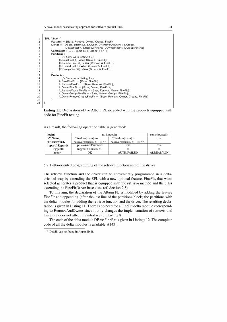
The retrieve function and the driver can be conveniently programmed in a delta-oriented way by extending the SPL with a new optional feature, FineFit, that whenselected generates a product that is equipped with the retrieve method and the classextending the FineFitDriver base class (cf. Section 2.3).
To this aim, the declaration of the Album PL is modified by adding the featureFineFit and appending (after the last line of the partitions-block) the partitions withthe delta modules for adding the retrieve function and the driver. The resulting decla-ration is given in Listing 11. There is no need for a FineFit delta module correspond-ing to RemoveAndOwner since it only changes the implementation of remove, andtherefore does not affect the interface (cf. Listing 8).
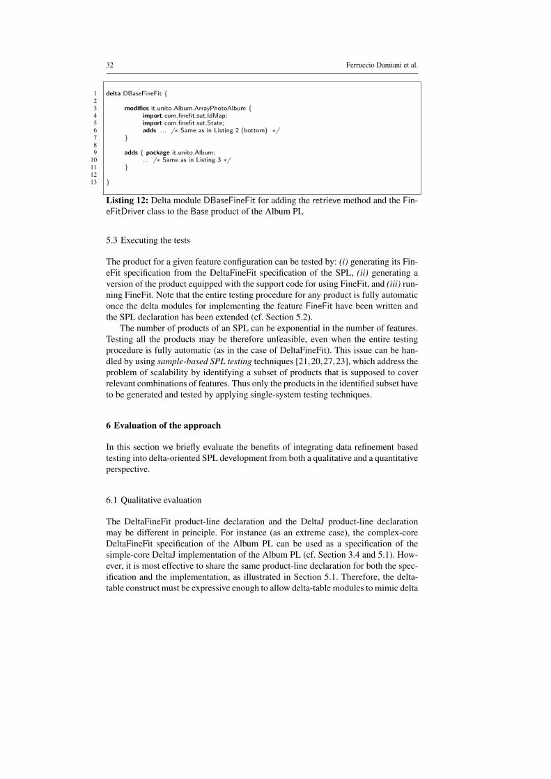
The code of the delta module DBaseFineFit is given in Listings 12. The completecode of all the delta modules is available at [43].
16 Details can be found in Appendix B.
32 Ferruccio Damiani et al.
1 delta DBaseFineFit {23 modifies it.unito.Album.ArrayPhotoAlbum {4 import com.finefit.sut.IdMap;5 import com.finefit.sut.State;6 adds ... /∗ Same as in Listing 2 (bottom) ∗/7 }89 adds { package it.unito.Album;
10 ... /∗ Same as in Listing 3 ∗/11 }1213 }
Listing 12: Delta module DBaseFineFit for adding the retrieve method and the Fin-eFitDriver class to the Base product of the Album PL
5.3 Executing the tests
The product for a given feature configuration can be tested by: (i) generating its Fin-eFit specification from the DeltaFineFit specification of the SPL, (ii) generating aversion of the product equipped with the support code for using FineFit, and (iii) run-ning FineFit. Note that the entire testing procedure for any product is fully automaticonce the delta modules for implementing the feature FineFit have been written andthe SPL declaration has been extended (cf. Section 5.2).
The number of products of an SPL can be exponential in the number of features.Testing all the products may be therefore unfeasible, even when the entire testingprocedure is fully automatic (as in the case of DeltaFineFit). This issue can be han-dled by using sample-based SPL testing techniques [21,20,27,23], which address theproblem of scalability by identifying a subset of products that is supposed to coverrelevant combinations of features. Thus only the products in the identified subset haveto be generated and tested by applying single-system testing techniques.
6 Evaluation of the approach
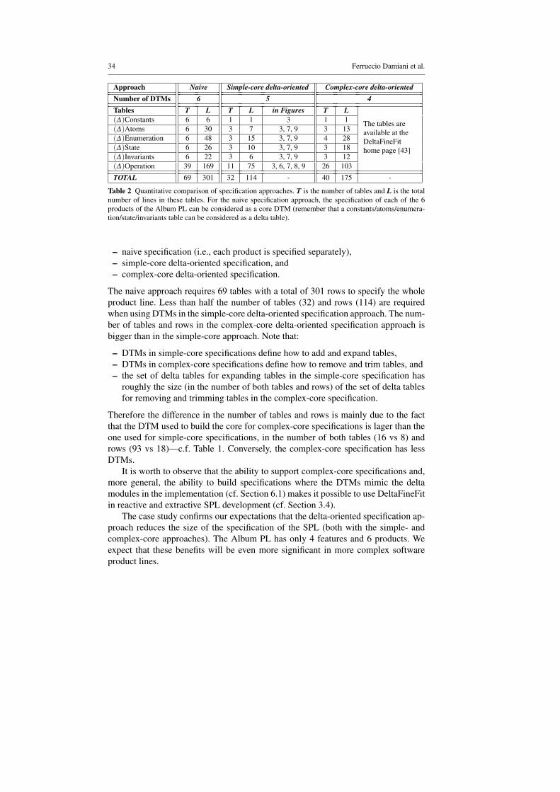
In this section we briefly evaluate the benefits of integrating data refinement basedtesting into delta-oriented SPL development from both a qualitative and a quantitativeperspective.
6.1 Qualitative evaluation
The DeltaFineFit product-line declaration and the DeltaJ product-line declarationmay be different in principle. For instance (as an extreme case), the complex-coreDeltaFineFit specification of the Album PL can be used as a specification of thesimple-core DeltaJ implementation of the Album PL (cf. Section 3.4 and 5.1). How-ever, it is most effective to share the same product-line declaration for both the spec-ification and the implementation, as illustrated in Section 5.1. Therefore, the delta-table construct must be expressive enough to allow delta-table modules to mimic delta
A novel model-based testing approach for software product lines 33
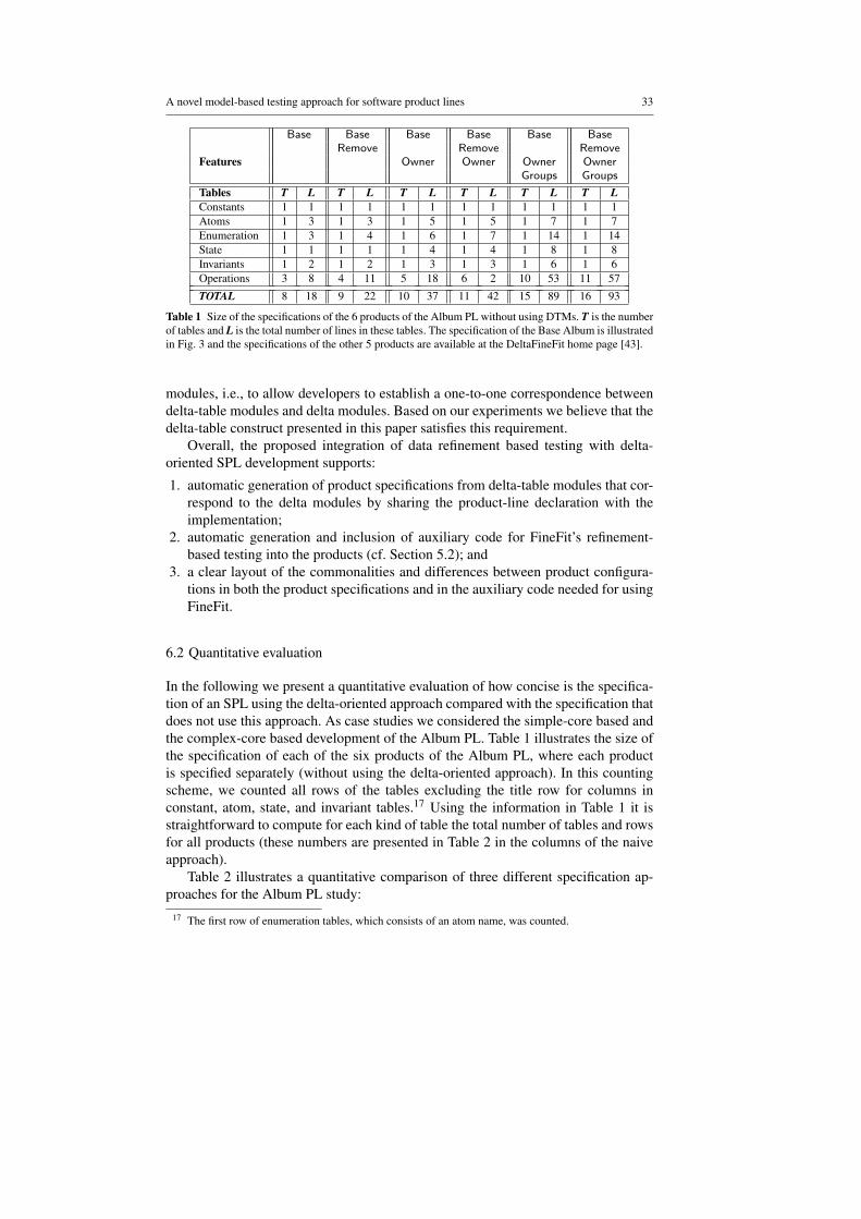
Features
Base Base Base Base Base BaseRemove Remove Remove
Owner Owner Owner OwnerGroups Groups
Tables T L T L T L T L T L T LConstants 1 1 1 1 1 1 1 1 1 1 1 1Atoms 1 3 1 3 1 5 1 5 1 7 1 7Enumeration 1 3 1 4 1 6 1 7 1 14 1 14State 1 1 1 1 1 4 1 4 1 8 1 8Invariants 1 2 1 2 1 3 1 3 1 6 1 6Operations 3 8 4 11 5 18 6 2 10 53 11 57
TOTAL 8 18 9 22 10 37 11 42 15 89 16 93
Table 1 Size of the specifications of the 6 products of the Album PL without using DTMs. T is the numberof tables and L is the total number of lines in these tables. The specification of the Base Album is illustratedin Fig. 3 and the specifications of the other 5 products are available at the DeltaFineFit home page [43].
modules, i.e., to allow developers to establish a one-to-one correspondence betweendelta-table modules and delta modules. Based on our experiments we believe that thedelta-table construct presented in this paper satisfies this requirement.
Overall, the proposed integration of data refinement based testing with delta-oriented SPL development supports:
1. automatic generation of product specifications from delta-table modules that cor-respond to the delta modules by sharing the product-line declaration with theimplementation;
2. automatic generation and inclusion of auxiliary code for FineFit’s refinement-based testing into the products (cf. Section 5.2); and
3. a clear layout of the commonalities and differences between product configura-tions in both the product specifications and in the auxiliary code needed for usingFineFit.
6.2 Quantitative evaluation
In the following we present a quantitative evaluation of how concise is the specifica-tion of an SPL using the delta-oriented approach compared with the specification thatdoes not use this approach. As case studies we considered the simple-core based andthe complex-core based development of the Album PL. Table 1 illustrates the size ofthe specification of each of the six products of the Album PL, where each productis specified separately (without using the delta-oriented approach). In this countingscheme, we counted all rows of the tables excluding the title row for columns inconstant, atom, state, and invariant tables.17 Using the information in Table 1 it isstraightforward to compute for each kind of table the total number of tables and rowsfor all products (these numbers are presented in Table 2 in the columns of the naiveapproach).
Table 2 illustrates a quantitative comparison of three different specification ap-proaches for the Album PL study:
17 The first row of enumeration tables, which consists of an atom name, was counted.
34 Ferruccio Damiani et al.
Approach Naive Simple-core delta-oriented Complex-core delta-orientedNumber of DTMs 6 5 4Tables T L T L in Figures T L
The tables areavailable at theDeltaFineFithome page [43]
Table 2 Quantitative comparison of specification approaches. T is the number of tables and L is the totalnumber of lines in these tables. For the naive specification approach, the specification of each of the 6products of the Album PL can be considered as a core DTM (remember that a constants/atoms/enumera-tion/state/invariants table can be considered as a delta table).
– naive specification (i.e., each product is specified separately),– simple-core delta-oriented specification, and– complex-core delta-oriented specification.
The naive approach requires 69 tables with a total of 301 rows to specify the wholeproduct line. Less than half the number of tables (32) and rows (114) are requiredwhen using DTMs in the simple-core delta-oriented specification approach. The num-ber of tables and rows in the complex-core delta-oriented specification approach isbigger than in the simple-core approach. Note that:
– DTMs in simple-core specifications define how to add and expand tables,– DTMs in complex-core specifications define how to remove and trim tables, and– the set of delta tables for expanding tables in the simple-core specification has
roughly the size (in the number of both tables and rows) of the set of delta tablesfor removing and trimming tables in the complex-core specification.
Therefore the difference in the number of tables and rows is mainly due to the factthat the DTM used to build the core for complex-core specifications is lager than theone used for simple-core specifications, in the number of both tables (16 vs 8) androws (93 vs 18)—c.f. Table 1. Conversely, the complex-core specification has lessDTMs.
It is worth to observe that the ability to support complex-core specifications and,more general, the ability to build specifications where the DTMs mimic the deltamodules in the implementation (cf. Section 6.1) makes it possible to use DeltaFineFitin reactive and extractive SPL development (cf. Section 3.4).
The case study confirms our expectations that the delta-oriented specification ap-proach reduces the size of the specification of the SPL (both with the simple- andcomplex-core approaches). The Album PL has only 4 features and 6 products. Weexpect that these benefits will be even more significant in more complex softwareproduct lines.
A novel model-based testing approach for software product lines 35
7 Related Work
The use of a tabular notation to specify operations was inspired by Parnas [32]. Tab-ular expressions can be represented and interpreted in many ways. Parnas proposesprecise definitions for ten varieties of tabular expressions [32]. We use the simple andintuitive Vector Function Tables to describe functions.
Various surveys deal with testing in SPLs; e.g., [16,30,25,8]. Delta tables lever-age the idea of tabular notation to the specification of product lines. To the best of ourknowledge this idea has not been proposed yet. The only papers introducing similaroperations on tables, also named delta tables, describe updates or views on database,e.g. [35]. However, it seems that this idea has not been proposed before to specifyprograms.
The approach proposed by Uzuncaova et al. [42] seems the most related to ourtesting approach. The paper describes a scope-bounded testing technique for pro-grams in an SPL developed by using the feature oriented programming (FOP) ap-proach (cf. Section 1 and Section 3.4). In the FOP approach a program is a com-position of feature modules, where each module implements an increment in thefunctionality of the program corresponding to a feature. This testing approach dif-fers from ours as their test suite enables only to add features, whereas we allow alsoto remove features. Hence, the test suite in [42] is monotonically extended with eachadditional feature. Using the Alloy Analyzer, tests are generated and the correctnessof the program is checked. Each feature F is specified as an Alloy formula, and theAlloy specification of a product is the conjunction of the specifications for its fea-tures. To generate larger inputs, tests are generated incrementally, as the analyzer isused each time on partial specifications rather than on the complete specification ofthe program. First the analyzer solves the specification for the Base feature (whichcorresponds to the base product), and the created relations are used when running theanalyzer on the specification of a feature F that is composed with Base. In our ap-proach, we generate both the program and its specification using the DOP approach,where a product is generated from another one by applying a delta-operation thatmay add or remove functionalities. The tests are then generated by considering thecomplete specification of a product. However, when a program is a composition offeatures, i.e., when the delta-modules do not use the remove operation, it should bepossible to apply our approach by using the incremental approach as in [42].
More recently, Lochau et al. [29,28] proposed a model-based SPL testing frame-work that is based on a delta-oriented SPL test model and on regression-based testartifact generation. The framework comprises state machines as test models extendedwith delta-oriented modeling concepts to express variability. The framework is aimedto capture reuse potential, reusing both (i) test cases for different product variants,and (ii) test results across different products. In our framework no reuse of test casesor test results is currently supported. We believe that the technique proposed in [28]could be applicable also to our approach, although we are using a different specifica-tion language (Parnas tables).
Proof systems for the verification of delta-oriented SPLs have been recently pro-posed [18,11]. These approaches are related to ours since they use DOP to generatea product together with its specification; however, they aim at a formal verification.
36 Ferruccio Damiani et al.
Hahnle and Schaefer [18] presented a verification approach for DOP that relies onthe Liskov principle for DOP, i.e, the specification of a method modified by a deltamodule must entail the specification of the previous versions of the method. This en-sures that each delta module can be verified by approximating called methods thatare defined in other delta modules by the specification of their first introduction. Inorder to relax the restriction imposed by the Liskov principle for DOP [18], Damianiet-al. [11] suggest to use symbolic assumptions on called methods in order to sepa-rate the specifications of method implementations from the requirements to methodcalls in a way which is similar to lazy behavioral subtyping [15]. The idea is to verifyfirst each delta module in isolation, based on symbolic assumption for methods callsthat may be defined in other delta modules, and then to verify each product based onthe already established specification for the used delta modules. The combination ofsoftware verification and testing techniques is encouraged due to their complemen-tary strengths. We believe that some ideas for combining verification and testing thatalready had been implemented for a single system (see [6]) could be applied to SPLs.
8 Conclusion and Future Work
We illustrated how the FineFit approach can be integrated into DOP to support the de-velopment of correct software product lines. Refinement-based testing is completelyintegrated into the delta-oriented SPL development process. Delta-oriented program-ming is used not only to generate the system under test, but also to generate theFineFit specification, the retrieve function and the driver for each product.
We would like to complete the development of the DeltaFineFit tool chain. Inparticular, we would like to improve the tool support for the delta-oriented program-ming of the retrieve function and the driver by developing a tabular notation that willbe automatically translated into the corresponding delta modules.
A type system for DOP, formalized for the minimal core calculus IMPERATIVEFEATHERWEIGHT DELTA JAVA(IF∆J) [7], guarantees that if an IF∆J product line iswell-typed then its product generation mapping is total and all its products are well-typed Java programs (cf. Section 3.3). In future work we plan to formalize a suitablenotion of well-formed FineFit specification and to develop static analysis techniquesfor checking whether the product generation mapping of a DeltaFineFit specifica-tion is total and all its products are well-formed FineFit specifications. Moreover, wewould like to extend the DeltaFineFit approach to deal with dynamic DOP [13,12].
We also plan to develop case studies to assess the effectiveness of using DeltaFin-eFit with sample-based SPL testing techniques (see Section 5.3), and to enhanceDeltaFineFit by exploring both the use of techniques for reusing test cases or testresults similar to [28] (cf. Section 7) and the use of test prioritization techniques sim-ilar to [26]. Another enhancement of DeltaFineFit that we would like to explore isthe integration of verification techniques (see the discussion at the end of Section 7).
Acknowledgements We thank the anonymous referees of PPPJ’13 for valuable comments on a prelimi-nary version of this paper and the anonymous SoSyM referees for many insightful comments and sugges-tions for improving the paper.
A novel model-based testing approach for software product lines 37
A The structure and semantics of operation tables
A FineFit operation table is a predicate that specifies the behavior of an operation as a relation betweenthe model’s state variables before the operation starts (the pre state) and after the operation completes (thepost state). It consists of two major areas: an expression table and a precondition tree. The expression tableis a set of columns, where each column defines the values of the state variables in the post state, given theirvalues in the pre state. The predcondition tree consists of predicates that determine which columns to usein the definition of the post state. For example, consider the following operation table:
R(c?:Int) c?≤ 0 c? > 0x < 0 x≥ 0 true
x = 0 x+ c?y = 0 x+ y
The operation R has a single input parameter c? and determines the value of its two state variablesx and y as follows: If c? is positive then the operation must set x to x+ c? and y to x+ y (the right mostcolumn), otherwise, if c? is not positive, the effect of the operation depends on the current value of x. Whenx is not negative x and y must be set to zero and when x is negative then x and y do not change (their valuemust be the same as it was when the operation started). Note that the predicate for determining whethercolumns 1 and 218 are relevant for the specification is the conjunction of the child predicates x < 0 andx≥ 0 with their parent predicate c?≤ 0.
We now define the conditions necessary for the precondition part of the table to form a tree. Considerthe precondition part of the table as a matrix of cells. Then, each predicate spans one or more consecutivecells (in the same row) and the space that each predicate occupies must be included below the space that itsparent (the predicate above) occupies. For example, the predicate x≥ 0 occupies cell (2,2) and its parent,the predicate c?≤ 0 occupies cells (1,1),(1,2).
Formally, consider a precondition part that is arranged in a matrix of n rows by m columns of cells.The i-th row contains a sequence of predicates, each occupying a span of one or more cells. Let ki indicatethe sequence of spans that each predicate occupies (and therefore ki j is the j-th span in the i-th row).For example, in the operation above, k1 = 2,1 and k2 = 1,1,1. In order for the spans to describe a validprecondition tree, three conditions must be met:
1. The sum of spans in each row must be equal to the number of columns in the matrix:
|ki |
∑j=1
ki j = m
where |ki| is the number of elements in the ith sequence of spans.2. The cells that each predicate spans must be included below the span of cells of its parent:
Si j ⊆ S(i−1)l for some 1≤ l ≤ m
where the span of cells of the j-th predicate in the i-th row is
Si j =j−1
∑l=1
kil +1, . . . ,j
∑l=1
kil
3. The last row (n) must consist of individual cells, that is
kn j = 1 for all 1≤ j ≤ m.
This arrangement ensures that the predicates form a tree structure19 with m leaves, all occupying thelast row. The following matrix illustrates this structure:
18 We do not count the left most column containing the state variables.19 In fact this is a forest. However, it can be transformed into a tree by adding an imaginary true as the
parent of the predicates at the first row.
38 Ferruccio Damiani et al.
1 2 3 4 5 6 7
3
2
1
There are three span sequences, one for each row:
k3 = 1,1,1,1,1,1,1 (3)
k2 = 3,2,2 (4)
k1 = 5,2 (5)
We can see that each span is included below the span of its parent. For example,
S2,2 = {4,5} ⊆ S1,1 = {1,2,3,4,5}
We say that the precondition tree is well formed when it satisfies the three conditions we have definedabove. In the rest of the discussion we always assume that we are working with well formed preconditiontrees. Given a column i we define the guard for this column as the conjunction of the leaf that occupies thei-th column and all its ancestors. Let v′ = v′1, . . . ,v
′l be the state space vector. Let ci be the i-th column of
the expression table. Then the meaning of the operation specification is:
v′ ∈ {ci : 1≤ i≤ m∧guard(i)}That is, the value of the state variables vector in the post state can be equal to the value of any of theexpression table columns whose guard was true in the pre state.The semantics of individual predicates and expressions is explained in [17].
B The algorithm that computes the apply function
We provide (in Section B.1) a Haskell executable specification of the apply function (cf. Section 4.2.1),and present (in Section B.2) its Java implementation. Note that in this paper all the tables resulting fromdelta-table application have been generated using this implementation.
B.1 Executable specification in Haskell
The executable specification of the algorithm that computes the apply function is provided as a programwritten in Haskell (Listing 13). Haskell is a functional programming language with a syntax that stronglyresembles the usual mathematical notation for defining function by cases, via pattern matching.
The Haskell code and the comments in Listing 13 should be almost self-explanatory. In the following,we shortly explain some technicalities. The expression contained in an ordinary table cell and in a deltatable cell containing the insert or replace operators is represented using the standard library type String(Line 4). Both ordinary tables and delta tables are represented as trees, where each node corresponds to acell. A tree that represents a table (ordinary or delta) is expressed as a value of the recursive data type Table(Line 11)—a value of type Table describes the root cell and the list of its immediate subtrees. The datatype Table has five data constructors (each describes a different kind of node): Basic, Insert, and Replace
A novel model-based testing approach for software product lines 39
(all have arity two), Match and Remove (arity one).20 Ordinary tables are represented by using only thedata constructor Basic, while delta tables are represented by using only the other data constructors, whichcorrespond to the delta table operators.
Example 3 (Representation of ordinary tables and delta tables in Haskell) Since ordinary tables mayhave more than one cell in their first row, they are always encoded by adding a top node containing thestring “ROOT”. Delta tables are therefore encoded by adding a top node containing the match operator(matching the top node in the ordinary tables). The following ordinary and delta tables
AC D1 2i ii
∗II IJ− ∗ ∗ −− ∗ ∗IX −− ∗ ∗IY −
are respectively represented by the following values of type Table:
The Haskell function apply (Lines 16-51) corresponds to the apply function (introduced in Sec-tion 4.2.1) that executes the delta operations of the delta table. To improve readability we have not modeledthe behavior described in Remark 2 of Section 4.2.1.
Line 26 declares the type of the apply function. The first argument of the function apply has typeMaybe Table. The standard library Maybe data type has two constructors: the unary data constructorJust and the constant Nothing. It is used to specify optional values: a value of type Maybe Table eithercontains a table t (represented as Just t), or it is empty (represented as Nothing).
The standard library function concat takes two lists and returns their concatenation. The standardlibrary function zipWith calls a given function pairwise on each member of both lists, returning a list. Forthe convenience of readers zipWith’s code is as follows:
zipWith :: (a −> b −> c) −> [a] −> [b] −> [c]zipWith [] = []zipWith [] = []zipWith f (x:xs) (y:ys) = (f x y) : zipWith f xs ys
Example 4 (An execution of the Haskell function apply) Consider the following delta table application,which already has been presented at the end of Section 4.2.1 (recall that the numbers to the left of the cellsdenote the recursion step):
1: A2,3: C
4: 15: i6: w
apply
1: ∗2: II3: ∗4: ∗ID5: −6: ∗
yields
1: A2: I3: C4: D6: w
The above delta table application can be defined by appending to the code in Listing 13 the following threelines:21
t = Basic "ROOT" [Basic "A" [Basic "C" [Basic "l" [Basic "i" [Basic "w" []]]]]]dt = Match [Match [Insert "I" [Match [Remove [Insert "D" [Remove [Match []]]]]]]]main = print (apply Nothing t dt)
20 Adding deriving(Show) at the end of a data declaration enables printing instances on standard output.21 Adding a definition for the name main makes Listing 13 a complete program.
40 Ferruccio Damiani et al.
1 module Main where234 type Expr = String567 −− |A table is a tree that consists of the following nodes:8 −− 1. Basic nodes that represent the expressions in Finefit tables.9 −− 2. Match, Remove, Insert, and Replace nodes, that represent the operations of the delta tables.
1011 data Table = Basic Expr [Table]12 | Match [Table] | Remove [Table] | Insert Expr [Table] | Replace Expr [Table]13 deriving(Show)141516 −− |We assume that the tables given to the apply function, have a correct structure. For example, that each17 −− table is a tree rooted at a dummy node, the original table has only basic expression nodes, and so on.18 −− The complete system checks that the tables have the correct structure, adding these checks to the19 −− specification would hinder understanding the essential ideas.20 −− The apply function takes the following arguments:21 −− 1. the parent of the node in the original table (or the constant Nothing, if the node is the root),22 −− 2. the node itself,23 −− 3. the corresponding node in the delta table.24 −− The function returns the sequence of nodes that corresponds to the new table.2526 apply :: Maybe Table −> Table −> Table −> [Table]2728 −− |Some notes on the recursive specification of the function:29 −− 1. We divide the specification into several cases by pattern matching on the kinds of delta table nodes30 −− (each kind of delta table operator node has its own case).31 −− 2. In all cases, we take care to pass the correct parent for the nodes in the recursive call.32 −− Applying a delta table match operator to a node of the original table, keeps the content of the original33 −− table, and recursively applies the children of the match node, to those of the original node.3435 apply node (Match deltas) = [Basic (content node) (apply to children node deltas)]3637 −− |Applying a delta table remove to a node of the original table, replaces the node by its children38 −− (after they are transformed by the children of the delta table node).39 −− This case is the reason why apply returns a list of tables.4041 apply node (Remove deltas) = apply to children node deltas4243 −− |Applying a delta table insert to a node of the original table, inserts a new node as the child of the44 −− original node’s parent, and all of the parent’s children (including the original node) as the children of45 −− the newly inserted node.4647 apply (Just parent) (Insert e’ deltas) = [Basic e’ (apply to children parent deltas)]4849 −− Replace is implemented in terms of remove followed by insert5051 apply p x (Replace e cs) = apply p x (Insert e [Remove cs])525354 −− |To process the children of a table node against a sequence of delta table operators, we traverse both55 −− lists, calling apply on each pair of corresponding nodes. This generates a list of lists, that we then56 −− concatenate to form the result.5758 apply to children parent deltas = concat (zipWith (apply (Just parent)) (children parent) deltas)5960 children :: Table −> [Table]61 children (Basic xs) = xs6263 content :: Table −> Expr64 content (Basic c ) = c
Listing 13: Executable specification of the algorithm that computes the apply func-tion introduced in Section 4.2.1; the behavior described in Remark 2 is not modeled
A novel model-based testing approach for software product lines 41
B.2 The Java implementation
The Java implementation of the algorithm that computes the apply function is given in Listings 14 and 15.A cell of a table is represented by the Node class which extends the Vector class. Tables are representedas trees, and an object of class Node represents a cell, which is the root of a subtree, and contains (in theVector’s elements) the reference to the roots of the immediate subtrees.
The applyPrime method (Lines 16–21 in Listing 14) corresponds to the apply′ function (introduced inSection 4.3). It first calls (Line 17) the prepare method (which applies the rules described in Section 4.3),and then invokes (Line 19) the apply method (Lines 29–58 in Listing 14). The apply method correspondsto the apply function (introduced in Section 4.2.1 and specified in Section B.1). When calling the applymethod, the this object is the current node of the delta table, and orig and res are the current nodes of theoriginal table and of the resulting table, respectively.
The body of the apply method implements the recursive walking of the parse tree, which is controlledby the operations in the cells of the delta table and, therefore, describes how each operation works. Thefirst part of the method (Lines 31–44) reads the operation of the current delta node and updates the contentof the resulting node; Lines 35–40 implement the behavior described in Remark 2 of Section 4.2.1. Thesecond part of the method (Lines 46–56) is responsible for the recursive call.22 At each recursive call(Lines 37, 50, and 54) the method getOrCreateChild(i), which creates the nodes of the resulting table, iscalled; it either returns the i-th subnode if it already exists, or it creates the i-th subnode and returns it. Wenow continue illustrating the apply method using small examples. (An example of an execution trace ofthe method apply is provided in Example 5.)
The loop that begins in Line 46 iterates over the siblings of the current delta table node. This meansthat if at the current level the original table has more cells than the delta table, then the additional cells areignored. For example:
A B C apply ∗ ∗ yields A B
If the delta table has more cells than the original table at the current level, the last cell of the original tableis repeatedly used when processing the additional operations of the delta table (Line 53). For example:
A B apply ∗ ∗ ∗ yields A B B
If the original table contains no cells at the current level and the current operation of the delta table is ∗ or−, the remaining operations of the delta table on the current branch are ignored (Line 52).
A apply∗∗ yields A
If the original table contains no cells at the current level and the current operation of the delta table is I or∗I, a cell with the value of the insert or replace operations is inserted (Line 50) in the resulting table. Line47 maps in this case the replace operation to an insert operation. For example:
A apply∗IB∗IC
yieldsABC
It is therefore possible to extend a table with new variable and value rows by using either the insert orreplace operation.
The algorithm traverses the original table and the delta table in parallel. The recursive call in Line 54is responsible for the operations match, remove, and replace 23. The recursive call in Line 50 handles theinsert operation, where the current node of the original table is passed as the first argument rather than thecurrent child of the original table. Delaying the recursive step on the original table results in the describedsemantics of the insert operation.
The recursive call in Line 37 is used for convenience. If either the remove or the match operation occuras the last condition in a condition hierarchy, but the condition cell c of the original table has additionalsubconditions (this is checked by isLastConditionNode()), the remove or the match operation is appliedto all subcondition of c. For example, let A,B, and C be condition cells, then
22 Line 37 is a special case, where ∗ matches multiple condition cells.23 If replace is not substituted by insert in Line 47.
42 Ferruccio Damiani et al.
1 import java.util.Vector;23 /∗ The Node class represents a cell of a table. Subnodes represent cells below this cell. ∗/45 public class Node extends Vector<Node>{67 public enum Op {nop,match,remove,insert,replace};8 public Op op = Op.nop; //Default is no operation9 public String val = ""; //Value or content of the cell
10 public boolean cond = false; //true if this node is a condition node and not a value node1112 public Node(String val){this.val=val;}131415 /∗ ”this” represents the root of the delta table. ”orig” is the root of the original table. ∗/16 public Node applyPrime(Node orig){ //corresponds to the function apply′ of Section 4.317 prepare(orig, this);18 Node result = new Node("<root>");19 apply(orig, result);20 return result;21 }222324 public static void prepare(Node orig, Node delta){...} //See Section 4.3252627 /∗ The parameters ”this”, ”orig”, and ”res” represent the current node (or cell) of the28 delta table, original table, and resulting table, respectively. ∗/29 public void apply(Node orig, Node res){ //corresponds to the function apply of Section 4.2.13031 switch(op){32 case nop: break;33 case remove: res.op = Op.remove; //no break here34 case match: res.val = unifyValue(orig.val);35 if(isLastConditionNode() && !orig.isLastConditionNode()){ //see Remark 2 in Section 4.2.136 for(int i=0; i<orig.size(); i++){37 apply(orig.get(i), res.getOrCreateChild(i, cond));38 }39 return;40 }41 break;42 case insert: res.val = val; break;43 case replace: res.val = val; break;44 }4546 for(int i=0; i<size(); i++){47 if(orig.size()==0 && get(i).op==Op.replace){ get(i).op=Op.insert; }4849 if(get(i).op==Op.insert){50 get(i).apply(orig, res.getOrCreateChild(i, cond));51 }else{52 if(orig.size()==0) break;53 Node newOrig = (i<orig.size()? orig.get(i) : orig.lastElement() );54 get(i).apply(newOrig, res.getOrCreateChild(i, cond));55 }56 }57 res.deleteTemporaryRemoveNodes();58 } // end of method apply596061 ... //See Listing 156263 } // end of class Node
Listing 14: Java implementation of the algorithms that compute the apply′ and applyfunctions
A novel model-based testing approach for software product lines 43
1 /∗ Returns true if this node is a condition node and its child nodes are non−condition (value) nodes.∗/2 public boolean isLastConditionNode(){3 if(!cond) return false;4 if(size()==0) return true;5 if(get(0).cond) return false; //For simplicity only one child is checked.6 return true;7 }89 /∗ Returns the i’th subnode. If the subnode does not exist, then it is create and returned. ∗/
10 public Node getOrCreateChild(int i, boolean cond){11 if(i<size()){12 return get(i);13 }else{14 Node tmp = new Node("");15 tmp.cond = cond;16 tmp.op = Op.nop;17 add(tmp);18 return getOrCreateChild(i, cond);19 }20 }2122 /∗ Replaces each child of this node that is marked as remove ”−” by its grand children.23 The algorithm operates recursively until no child is marked with remove ”−”.∗/24 protected void deleteTemporaryRemoveNodes(){25 boolean childRemoved=false;26 do{27 childRemoved=false;28 for(int i=0; i<size();i++){29 Node child = get(i);30 if(child.op==Node.Op.remove){ //Replace the removed child by its children31 remove(i);32 for(int j=i,k=0; k<child.size();k++,j++){33 insertElementAt(child.get(k), j);34 }35 childRemoved = true;36 break;37 }38 }39 }while(childRemoved);40 }4142 /∗ if the delta value is ”∗”, then origVal is returned. Otherwise all occurrences43 of ”∗” in the delta value are replace with origVal. E.g., ”x” apply ”(∗)+y” yields ”x+y”.∗/44 public String unifyValue(String origVal){45 if(val.equals("*"))46 return origVal;47 else48 return val.replaceAll("(*)",origVal);49 }
Listing 15: Helper methods of the apply method
AB C
apply ∗ yieldsA
B C
The reader may have noticed that unlike the other operations, the remove operation is not handledin the loop in Lines 46–56. When a remove operation occurs, a temporary cell is created in the resultingtable that is marked to be removed (Line 33). The marked cells are removed in Line 57. Removing nodesat the end of the recursion simplifies the implementation, because removing a node c pulls-up its childrenc1, . . . ,cn to the current level. Hence, by removing a node the number of siblings at the current level maydecrease, stay constant, or increase. In the following example we assume that A is not a condition cell.
A BC D E
apply ∗ − yields A D E
44 Ferruccio Damiani et al.
Example 5 (An execution trace of the method apply) For a complete example consider the followingdelta table application, which already has been presented at the end of Section 4.2.1 and in Example 4 ofAppendix B.1:
1: A2,3: C
4: 15: i6: w
apply
1: ∗2: II3: ∗4: ∗ID5: −6: ∗
yields
1: A2: I3: C4: D6: w
Executing the method apply in (Lines 29–58) will result in the following recursive invocations of themethod:
Recursion step this orig res
0 < root > < root > < root >1 ∗ A A2 II C I3 ∗ C C4 ∗ID 1 D5 − i −6 ∗ w w
At the end of the last recursion step of the apply algorithm (Line 57 in Listing 14) the methoddeleteTemporaryRemoveNodes is called which removes the temporary “−” node from the resultingtree res that is introduced at recursion step 5.
2. Apel, S., Kastner, C., Grosslinger, A., Lengauer, C.: Type safety for feature-oriented product lines.Automated Software Engineering 17(3), 251–300 (2010)
3. Apel, S., Kastner, C., Lengauer, C.: Feature featherweight java: A calculus for feature-oriented pro-gramming and stepwise refinement. In: Proceedings of the 7th International Conference on Genera-tive Programming and Component Engineering, GPCE ’08, pp. 101–112. ACM, New York, NY, USA(2008). DOI 10.1145/1449913.1449931
4. Batory, D.: Feature Models, Grammars, and Propositional Formulas. In: Proceedings of the Interna-tional Conference on Software Product Lines (SPLC), LNCS, vol. 3714, pp. 7–20. Springer (2005)
6. Beckert, B., Gladisch, C., Tyszberowicz, S., Yehudai, A.: KeYGenU: combining verification-basedand capture and replay techniques for regression unit testing. Int. J. Systems Assurance Engineeringand Management 2(2), 97–113 (2011)
7. Bettini, L., Damiani, F., Schaefer, I.: Compositional type checking of delta-oriented software productlines. Acta Informatica 50, 77–122 (2013)
8. do Carmo Machado, I., McGregor, J.D., Cavalcanti, Y.C., de Almeida, E.S.: On strategies for testingsoftware product lines: A systematic literature review. Information and Software Technology 56(10),1183 – 1199 (2014)
10. Damiani, F., Gladisch, C., Tyszberowicz, S.: Refinement-based testing of delta-oriented product lines.In: Proceedings of the 2013 International Conference on Principles and Practices of Programming onthe Java Platform: Virtual Machines, Languages, and Tools, PPPJ ’13, pp. 135–140. ACM, New York,NY, USA (2013). DOI 10.1145/2500828.2500841
A novel model-based testing approach for software product lines 45
11. Damiani, F., Owe, O., Dovland, J., Schaefer, I., Johnsen, E.B., Yu, I.C.: A transformational proofsystem for delta-oriented programming. In: Proceedings of the 16th International Software ProductLine Conference - Volume 2, SPLC ’12, pp. 53–60. ACM, New York, NY, USA (2012). DOI 10.1145/2364412.2364422
12. Damiani, F., Padovani, L., Schaefer, I.: A formal foundation for dynamic delta-oriented softwareproduct lines. In: Proceedings of the 11th International Conference on Generative Programming andComponent Engineering, GPCE ’12, pp. 1–10. ACM, New York, NY, USA (2012). DOI 10.1145/2371401.2371403
13. Damiani, F., Schaefer, I.: Dynamic delta-oriented programming. In: Proceedings of the 15th Interna-tional Software Product Line Conference, Volume 2, SPLC ’11, pp. 34:1–34:8. ACM, New York, NY,USA (2011). DOI 10.1145/2019136.2019175
14. Delaware, B., Cook, W.R., Batory, D.: Fitting the pieces together: A machine-checked model of safecomposition. In: Proceedings of the the 7th Joint Meeting of the European Software EngineeringConference and the ACM SIGSOFT Symposium on The Foundations of Software Engineering, ES-EC/FSE ’09, pp. 243–252. ACM, New York, NY, USA (2009). DOI 10.1145/1595696.1595733
16. Engstrom, E., Runeson, P.: Software product line testing - a systematic mapping study. Informationand Software Technology 53(1), 2–13 (2011)
17. Faitelson, D., Tyszberowicz, S.S.: Data refinement based testing. Int. J. Systems Assurance Engineer-ing and Management 2(2), 144–154 (2011)
18. Hahnle, R., Schaefer, I.: A Liskov Principle for Delta-Oriented Programming. In: Leveraging Appli-cations of Formal Methods, Verification and Validation. Technologies for Mastering Change Interna-tional Symposium (ISoLA), Part I, LNCS, vol. 7609, pp. 32–46. Springer (2012)
19. Jackson, D.: Software Abstractions - Logic, Language, and Analysis. MIT Press (2012)20. Johansen, M.F., Haugen, O., Fleurey, F.: Properties of realistic feature models make combinatorial
testing of product lines feasible. In: Proceedings of the International Conference on Model DrivenEngineering Languages and Systems (MODELS), pp. 638–652. Springer-Verlag, Berlin, Heidelberg(2011)
21. Johansen, M.F., Haugen, O., Fleurey, F.: An algorithm for generating t-wise covering arrays fromlarge feature models. In: Proceedings of the 16th International Software Product Line Conference -Volume 1, SPLC ’12, pp. 46–55. ACM, New York, NY, USA (2012). DOI 10.1145/2362536.2362547
22. Koscielny, J., Holthusen, S., Schaefer, I., Schulze, S., Bettini, L., Damiani, F.: Deltaj 1.5: Delta-oriented programming for java 1.5. In: Proceedings of the 2014 International Conference on Prin-ciples and Practices of Programming on the Java Platform: Virtual Machines, Languages, and Tools,PPPJ ’14, pp. 63–74. ACM, New York, NY, USA (2014). DOI 10.1145/2647508.2647512
23. Kowal, M., Schulze, S., Schaefer, I.: Towards efficient spl testing by variant reduction. In: Proceedingsof the 4th International Workshop on Variability & Composition, VariComp ’13, pp. 1–6. ACM, NewYork, NY, USA (2013). DOI 10.1145/2451617.2451619
24. Krueger, C.: Eliminating the Adoption Barrier. IEEE Software 19(4), 29–31 (2002)25. Lee, J., Kang, S., Lee, D.: A survey on software product line testing. In: Proceedings of the 16th
International Software Product Line Conference - Volume 1, SPLC ’12, pp. 31–40. ACM, New York,NY, USA (2012). DOI 10.1145/2362536.2362545
26. Li, Z., Harman, M., Hierons, R.M.: Search algorithms for regression test case prioritization. IEEETSE 33(4), 225–237 (2007)
27. Lochau, M., Goltz, U.: Feature interaction aware test case generation for embedded control systems.Electronic Notes in Theoretical Computer Science 264(3), 37–52 (2010)
28. Lochau, M., Lity, S., Lachmann, R., Schaefer, I., Goltz, U.: Delta-oriented model-based integrationtesting of large-scale systems. Journal of Systems and Software 91(0), 63 – 84 (2014)
29. Lochau, M., Schaefer, I., Kamischke, J., Lity, S.: Incremental model-based testing of delta-orientedsoftware product lines. In: TAP, LNCS, vol. 7305, pp. 67–82. Springer (2012)
30. da Mota Silveira Neto, P.A., do Carmo Machado, I., McGregor, J.D., de Almeida, E.S.,de Lemos Meira, S.R.: A systematic mapping study of software product lines testing. Informationand Software Technology 53(5), 407 – 423 (2011). Special Section on Best Papers from {XP2010}
31. Mugridge, R., Cunningham, W.: Fit for Developing Software: framework for integrated tests. PrenticeEducation, Inc. (2005)
32. Parnas, D.L.: Tabular representation of relations. Tech. Rep. 260, Research Institute of Ontario, Mc-Master University (1992)
46 Ferruccio Damiani et al.
33. Pohl, K., Bockle, G., van der Linden, F.: Software Product Line Engineering - Foundations, Principles,and Techniques. Springer (2005)
34. de Roever, W.P., Engelhardt, K.: Data Refinement: Model-oriented Proof Theories and their Com-parison, Cambridge Tracts in Theoretical Computer Science, vol. 46. Cambridge University Press(1998)
35. Salem, K., Beyer, K., Lindsay, B., Cochrane, R.: How to roll a join: Asynchronous incremental viewmaintenance. In: Proceedings of the 2000 ACM SIGMOD International Conference on Managementof Data, SIGMOD ’00, pp. 129–140. ACM, New York, NY, USA (2000). DOI 10.1145/342009.335393
36. Schaefer, I., Bettini, L., Bono, V., Damiani, F., Tanzarella, N.: Delta-oriented Programming of Soft-ware Product Lines. In: Software Product Line Conference (SPLC), LNCS, vol. 6287, pp. 77–91.Springer (2010)
37. Schaefer, I., Bettini, L., Damiani, F.: Compositional type-checking for delta-oriented programming.In: Proceedings of the Tenth International Conference on Aspect-oriented Software Development,AOSD ’11, pp. 43–56. ACM, New York, NY, USA (2011). DOI 10.1145/1960275.1960283
38. Schaefer, I., Damiani, F.: Pure delta-oriented programming. In: Proceedings of the 2Nd InternationalWorkshop on Feature-Oriented Software Development, FOSD ’10, pp. 49–56. ACM, New York, NY,USA (2010). DOI 10.1145/1868688.1868696
39. Schaefer, I., Rabiser, R., Clarke, D., Bettini, L., Benavides, D., Botterweck, G., Pathak, A., Trujillo,S., Villela, K.: Software diversity: state of the art and perspectives. International Journal on SoftwareTools for Technology Transfer 14(5), 477–495 (2012)
40. Spivey, J.M.: The Z Notation: A Reference Manual. Prentice Hall International (2001)41. Torlak, E., Jackson, D.: Kodkod: A relational model finder. In: Tools and Algorithms for the Con-
struction and Analysis of Systems (TACAS), LNCS, vol. 4424, pp. 632–647. Springer (2007)42. Uzuncaova, E., Khurshid, S., Batory, D.S.: Incremental test generation for software product lines.
IEEE TSE 36(3), 309–322 (2010)43. The DeltaFineFit home page. http://di.unito.it/deltafinefit44. The DeltaJ home page. https://www.tu-braunschweig.de/isf/research/deltas45. The FineFit home page. https://github.com/coderocket/finefit