1

A Novel Multiobjective Cell Switch-OffFramework for Cellular Networks

David Gonzalez G., Member, IEEE, Jyri Hamalainen, Member, IEEE,Halim Yanikomeroglu, Senior Member, IEEE, Mario Garcıa-Lozano and Gamini Senarath

Abstract—Cell Switch-Off (CSO) is recognized as a promisingapproach to reduce the energy consumption in next-generationcellular networks. However, CSO poses serious challenges notonly from the resource allocation perspective but also fromthe implementation point of view. Indeed, CSO represents adifficult optimization problem due to its NP-complete nature.Moreover, there are a number of important practical limitationsin the implementation of CSO schemes, such as the needfor minimizing the real-time complexity and the number ofon-off/off-on transitions and CSO-induced handovers. This arti-cle introduces a novel approach to CSO based on multiobjectiveoptimization that makes use of the statistical description of theservice demand (known by operators). In addition, downlink anduplink coverage criteria are included and a comparative analysisbetween different models to characterize intercell interferenceis also presented to shed light on their impact on CSO. Theframework distinguishes itself from other proposals in two ways:1) The number of on-off/off-on transitions as well as handoversare minimized, and 2) the computationally-heavy part of thealgorithm is executed offline, which makes its implementationfeasible. The results show that the proposed scheme achievessubstantial energy savings in small cell deployments where servicedemand is not uniformly distributed, without compromising theQuality-of-Service (QoS) or requiring heavy real-time processing.

Index Terms—Cellular networks, energy efficiency, cell switch-off, CSO, multiobjective optimization, Pareto efficiency.

I. INTRODUCTION

FUTURE hyper-dense small-cell deployments are expectedto play a pivotal role in delivering high capacity and

reliability by bringing the network closer to users [1]. How-ever, in order to make hyper-dense deployments a reality, en-hancements including effective interference management, self-organization, and energy efficiency are required [2]. Given thatlarge-scale deployments composed of hundreds or thousandsof network elements can increase the energy consumptionsubstantially, the need for energy efficiency (green communi-cations) has been recognized by the cellular communicationsindustry as an important item in research projects and stan-dardization activities [3, 4].

Initial attempts to improve the energy efficiency in cellularnetworks were oriented towards minimizing the power radiatedthrough the air interface, which in turn reduces the electro-magnetic pollution and its potential effects on human health.

David Gonzalez G. and Jyri Hamalainen are with the School ofElectrical Engineering at Aalto University, Finland. Corresponding email:david.gonzalez.g@ieee.org.

Halim Yanikomeroglu is with the Department of Systems and ComputerEngineering, Carleton University, Ottawa, Canada.

Mario Garcıa-Lozano is with the Department of Signal Theory and Commu-nications, Universitat Politecnica de Catalunya, Barcelona, Spain.

Gamini Senarath is with Huawei Canada R&D Centre.

However, most of the energy consumption (between 50% to80%) in the radio access network takes place in base sta-tions (BSs) [4] and it is largely independent of the BSs’ load.Since cellular networks are dimensioned to meet the servicedemand in the busy hour (i.e., peak demand), it is expectedthat, under non-uniform demand distributions (both in spaceand time), a substantial portion of the resources may end upbeing underutilized, thus incurring in an unnecessary expen-diture of energy. The problem may become worse in manyof the scenarios foreseen for 5G, presumably characterized byhyper-dense small-cell deployments, hierarchical architectures,and highly heterogeneous service demand conditions [5].Therefore, the idea of switching off lightly loaded base stationshas been considered recently as a promising method to reducethe energy consumption in cellular networks. This frameworkis referred to as Cell Switch-Off (CSO) and it is focused ondetermining the largest set of cells that can be switched offwithout compromising the Quality-of-Service (QoS) providedto users. Unfortunately, CSO is difficult to carry out due tothe fact that it represents a highly challenging (combinatorial)optimization problem whose complexity grows exponentiallywith the number of BSs, and hence, finding optimal so-lutions is not possible in polynomial time. Moreover, theimplementation of CSO requires coordination among neighborcells and several other practical aspects, such as coverageprovision and the need for minimizing the number of (induced)handovers and on-off/off-on transitions. In practice, optimizingthe number of transitions, as well as the time required for them,is advisable because switching on/off BSs is far from beinga simple procedure, and indeed, this process must be gradualand controlled [6, 7]. Moreover, a large number of transitionscould result in a high number of handovers with a potentiallynegative impact on QoS [8].

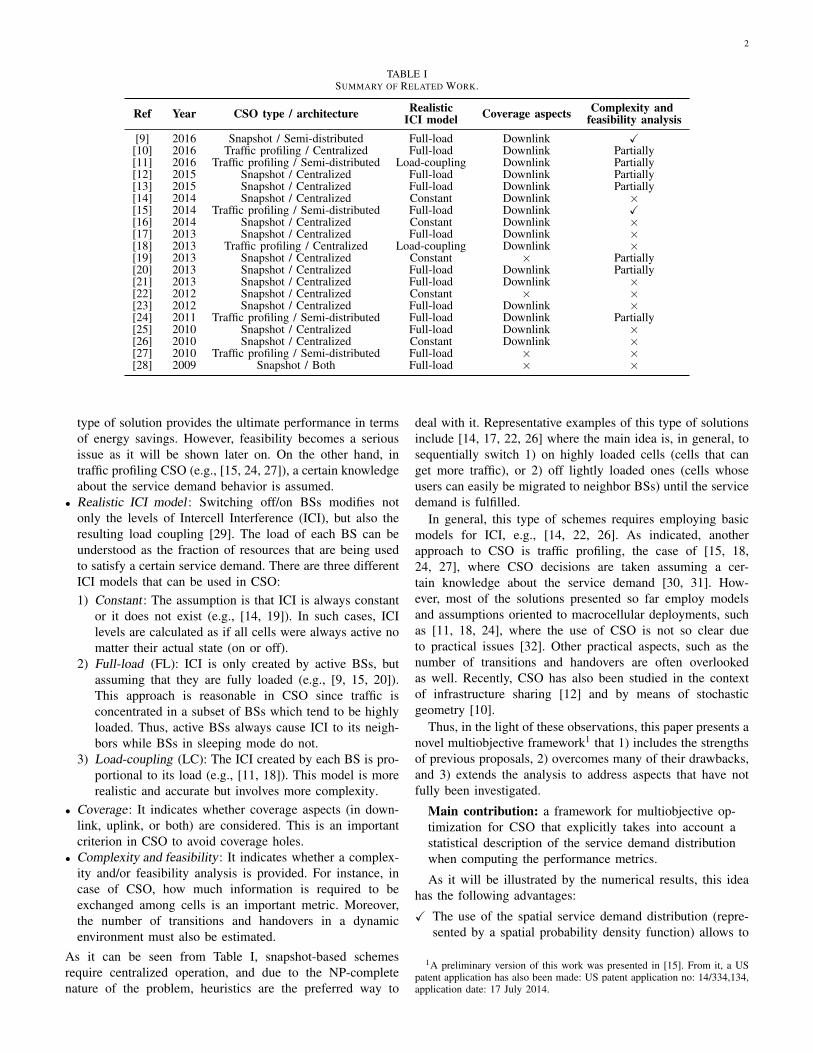
Although CSO is a relatively young research topic, asignificant amount of contributions has been made. Hence, anexhaustive survey is both out of the scope and not feasibleherein. Instead, a literature review including, in the opinion ofthe authors, some of the most representative works is provided.Thus, in the comparative perspective shown in Table I, thefollowing criteria have been considered:• CSO type / architecture: CSO solutions can be classified

as ‘snapshot’ or ‘traffic profiling’ CSO depending on theapproach followed to take the on/off decisions. In snapshotCSO (e.g., [14, 16, 17, 19]), decisions involve the analysis ofdiscrete realizations of users, i.e., whenever a CSO decisionis required, information of every single user in the networkneeds to be available at a central unit where an heuristic oroptimization procedure is performed. Given its nature, this

arX

iv:1

506.

0559

5v2

[cs

.NI]

4 N

ov 2

016

2

TABLE ISUMMARY OF RELATED WORK.

Ref Year CSO type / architecture Realistic Coverage aspects Complexity andICI model feasibility analysis

[9] 2016 Snapshot / Semi-distributed Full-load Downlink X[10] 2016 Traffic profiling / Centralized Full-load Downlink Partially[11] 2016 Traffic profiling / Semi-distributed Load-coupling Downlink Partially[12] 2015 Snapshot / Centralized Full-load Downlink Partially[13] 2015 Snapshot / Centralized Full-load Downlink Partially[14] 2014 Snapshot / Centralized Constant Downlink ×[15] 2014 Traffic profiling / Semi-distributed Full-load Downlink X[16] 2014 Snapshot / Centralized Constant Downlink ×[17] 2013 Snapshot / Centralized Full-load Downlink ×[18] 2013 Traffic profiling / Centralized Load-coupling Downlink ×[19] 2013 Snapshot / Centralized Constant × Partially[20] 2013 Snapshot / Centralized Full-load Downlink Partially[21] 2013 Snapshot / Centralized Full-load Downlink ×[22] 2012 Snapshot / Centralized Constant × ×[23] 2012 Snapshot / Centralized Full-load Downlink ×[24] 2011 Traffic profiling / Semi-distributed Full-load Downlink Partially[25] 2010 Snapshot / Centralized Full-load Downlink ×[26] 2010 Snapshot / Centralized Constant Downlink ×[27] 2010 Traffic profiling / Semi-distributed Full-load × ×[28] 2009 Snapshot / Both Full-load × ×

type of solution provides the ultimate performance in termsof energy savings. However, feasibility becomes a seriousissue as it will be shown later on. On the other hand, intraffic profiling CSO (e.g., [15, 24, 27]), a certain knowledgeabout the service demand behavior is assumed.

• Realistic ICI model : Switching off/on BSs modifies notonly the levels of Intercell Interference (ICI), but also theresulting load coupling [29]. The load of each BS can beunderstood as the fraction of resources that are being usedto satisfy a certain service demand. There are three differentICI models that can be used in CSO:1) Constant : The assumption is that ICI is always constant

or it does not exist (e.g., [14, 19]). In such cases, ICIlevels are calculated as if all cells were always active nomatter their actual state (on or off).

2) Full-load (FL): ICI is only created by active BSs, butassuming that they are fully loaded (e.g., [9, 15, 20]).This approach is reasonable in CSO since traffic isconcentrated in a subset of BSs which tend to be highlyloaded. Thus, active BSs always cause ICI to its neigh-bors while BSs in sleeping mode do not.

3) Load-coupling (LC): The ICI created by each BS is pro-portional to its load (e.g., [11, 18]). This model is morerealistic and accurate but involves more complexity.

• Coverage: It indicates whether coverage aspects (in down-link, uplink, or both) are considered. This is an importantcriterion in CSO to avoid coverage holes.

• Complexity and feasibility: It indicates whether a complex-ity and/or feasibility analysis is provided. For instance, incase of CSO, how much information is required to beexchanged among cells is an important metric. Moreover,the number of transitions and handovers in a dynamicenvironment must also be estimated.

As it can be seen from Table I, snapshot-based schemesrequire centralized operation, and due to the NP-completenature of the problem, heuristics are the preferred way to

deal with it. Representative examples of this type of solutionsinclude [14, 17, 22, 26] where the main idea is, in general, tosequentially switch 1) on highly loaded cells (cells that canget more traffic), or 2) off lightly loaded ones (cells whoseusers can easily be migrated to neighbor BSs) until the servicedemand is fulfilled.

In general, this type of schemes requires employing basicmodels for ICI, e.g., [14, 22, 26]. As indicated, anotherapproach to CSO is traffic profiling, the case of [15, 18,24, 27], where CSO decisions are taken assuming a cer-tain knowledge about the service demand [30, 31]. How-ever, most of the solutions presented so far employ modelsand assumptions oriented to macrocellular deployments, suchas [11, 18, 24], where the use of CSO is not so clear dueto practical issues [32]. Other practical aspects, such as thenumber of transitions and handovers are often overlookedas well. Recently, CSO has also been studied in the contextof infrastructure sharing [12] and by means of stochasticgeometry [10].

Thus, in the light of these observations, this paper presents anovel multiobjective framework1 that 1) includes the strengthsof previous proposals, 2) overcomes many of their drawbacks,and 3) extends the analysis to address aspects that have notfully been investigated.

Main contribution: a framework for multiobjective op-timization for CSO that explicitly takes into account astatistical description of the service demand distributionwhen computing the performance metrics.

As it will be illustrated by the numerical results, this ideahas the following advantages:

X The use of the spatial service demand distribution (repre-sented by a spatial probability density function) allows to

1A preliminary version of this work was presented in [15]. From it, a USpatent application has also been made: US patent application no: 14/334,134,application date: 17 July 2014.

3

the proposed algorithm to rapidly identify network topolo-gies, i.e., on/off patterns, providing higher capacity to areaswhere high service demand is more likely to appear, andhence, the search space and required computational effortis significantly reduced.

X Given that, in general, traffic profiles are stable in timescales of dozens of minutes, the (computationally-heavy)optimization can be done offline and required topologiescan be applied as needed as these traffic profiles arerecognized/observed during network operation. This fea-ture makes the implementation of CSO feasible, giventhat the required BS coordination and real-time processingare significantly reduced. However, the conceptual ideawill still be valid when new paradigms (cloud computing,software defined networking, and network virtualization,see [1]) allow faster computation and information exchangeamong network nodes. Thus, more dynamic traffic profilerecognition and optimization will also be possible underthe proposed framework.

X The proposed optimization formulation allows consideringseveral downlink and uplink coverage criteria, such asminimum received power and Signal to Interference plusNoise Ratio (SINR).

X Given that there exist a correlation between the topologiesthat are specific for a given traffic profile, the number ofhandovers and transitions is minimized.

Finally, the following set of secondary/minor contributionsare also presented in this work:1) Analysis of the impact of the most extended interference

models (FL and LC) on the performance of CSO.2) A quantitative assessment of how CSO operation affects

the critical uplink power consumption (on user equip-ment side). To the best of the authors’ knowledge, thisaspect/criterion has been overlooked in most of previousstudies, and only recently in [13] it has been integratedwithin an optimization framework.

3) While the multiobjective problem formulation presentedherein can be solved by means of standard stochastic opti-mization tools [33], an alternative iterative algorithm is alsoproposed for computing the important tradeoff between thenumber of active cells and network capacity. As it will beshown shortly, although its performance is slightly inferiorto stochastic search, it is significantly faster, and hence, itcould be used when real-time operation becomes feasible.

The rest of the paper is organized as follows: the next sectionpresents the system model. The proposed Multiobjective Opti-mization (MO) framework (performance metrics and problemformulation) is explained in Section III. Section IV describesthe evaluation setting and benchmarks used in simulations.Numerical results are also analyzed therein. Section V closesthe article with conclusions and research directions.

II. SYSTEM MODEL

A. Definitions and notations

In this study, an OFDMA cellular network is considered.The system bandwidth is B and the network is composed ofL BSs that can be independently switched off/on. The indices

of the BSs are contained in the set L = {0, 1, · · · , L−1}. Theset A, composed of A = |A| small area elements, representsthe spatial domain to which the network provides service. Itis assumed that within each area elements a ∈ A, the averagereceived power is constant. The maximum transmit power percell is Pmax. The network geometry is captured by the path lossmatrix G ∈ RA×L (distance dependent attenuation, antennagains, and shadowing). The vectors pPS and pD, both ∈ RL,indicate the transmit power at each cell in Pilot Signals (PS),and data channels, respectively. Cell selection is based on theaverage PS received power, which can be calculated by meansof the following expression:

RPS = G · diag (pPS � x) , RPS ∈ RA×L. (1)

The operator � denotes Hadamard (pointwise) operations.The vector x ∈ {0, 1}L indicates which cells are active andwhich ones are switched off. Hereafter, x is also referred toas ‘network topology’. Thus, the matrix RPS in (1) containsthe PS received power, i.e., RPS(a, l) indicates the receivedpower from the lth BS in the ath area element. Of interest isthe Number of Active Cells (NAC) in each network topologyas energy consumption is related to it. The ath area element(the ath row in RPS) is served by cell l? if

l? = argmaxl∈{0,1,... ,L−1}

RPS(a, l). (2)

The dependence of l? on x has not been explicitly indicated forthe sake of clarity. Based on (1) and (2), the binary coveragematrices S and Sc ∈ RA×L can be obtained. If the ath pixel isserved by l?, then S(a, l?) = 1. Sc is the binary complementof S. Hence, the coverage pattern, implicitly defined in S, isa function of x. The cell selection rule indicated by (2) canbe regarded as a connectivity function fc : A → L ∪ {−1}.If fc(a) = −1, the ath area element is out of coverage, i.e.,• the received power in a ∈ A (RPS (a, l?)) is smaller thanPRx

min, i.e., RPS (a, l?) ≤ PRxmin,

• the SINR (ψa) in the area element a ∈ A is smaller thanψmin, i.e., ψa ≤ ψmin, or

• the path loss G (a, l?) between the area element and itsserver is greater than GUL

max, i.e., G (a, l?) ≥ GULmax. In prac-

tice, GULmax is the maximum path-loss obtained from the

uplink link budget (a design criterion).The cell Al is the subset of A served by the lth BS. Thus,Al , { a ∈ A : fc(a) = l }, where Ai∩Aj = ∅, ∀ i 6= j. Theset Ac is the subset of A that are associated to one BS. Thus,Ac , { a ∈ A : fc(a) 6= −1} =

⋃l∈LAl. The vector Γ ∈ RA

corresponds to the spatial service demand distribution. Thus,Γ(a) indicates the probability, in the event of a new user, thatthe ath pixel has the user on it, and hence, ΓT ·1 = 1. It shouldbe noted that Γ is time-dependent, however it is reasonable toassume that Γ is constant during fixed intervals [30]. In orderto represent the service demand volume, two parameters areconsidered: inter-arrival time (λ) and session time (µ). Bothare modeled as exponentially distributed random variables.Thus, service demand’s spatial distribution and volume aredescribed by Γ and the first order statistics of λ and µ, i.e.,E{λ} and E{µ}, respectively. It is assumed that the QoS of a

4

user is satisfied if the target rate (rmin) is fulfilled. Hence, thetotal service demand volume (R) in A is given by

R =∑a∈A

ra [bps], (3)

wherera =

E{µ}E{λ}

· Γ(a) · rmin [bps] (4)

corresponds to the average demand in the ath area element. Theprevious model for the service demand can easily be extendedto the general case of more than one service to account withthe fact that service time, inter-arrival time, spatial distribution,and target rate can be service-specific. Assuming that there areNS service classes, each of them with different characteristics,i.e., µc, λc, Γc, and rcmin for c = 1, 2, · · · , NS, (4) can berewritten as follows:

rSa =

NS∑c=1

(E{µc}E{λc}

· Γc(a) · rcmin

)[bps]. (5)

The resulting spatial service demand distribution (that isrequired to compute the performance metrics introduced lateron) can be obtained by considering the resulting demand asfollows:

ΓS(a) =rSa∑

a∈A rSa

. (6)

Hereafter, one single service class (possibly the result of a mixof many others) is assumed for the sake of clarity, and hence,one single set of parameters (µ, λ, Γ, and rmin) are considered.

Definition II.1 (Cell load). The load of the lth BS (αl(t)), atany given time t, is defined as the fraction of the availableresources (bandwidth) that are being used.

The average load of the lth BS is αl , E{αl(t)}. Thus, thevector α = [ α0 α1 · · · αL−1 ] indicates the load conditionsin the network, on average. Note that if x(l) = 0, thenα(l) = 0. As the reader can easily infer, as long as α ≤ 1,the network topology (x) is able to satisfy, on average, theservice demand given by Γ, E{λ}, and E{µ}, and hence, itcan be said that x is adequate.

Definition II.2 (Network capacity). The network capacity(VCap) is defined as the maximum service demand volume suchthat α ≤ 1. Thus, VCap , max V : α ≤ 1.

Definition II.3 (Saturation point). The saturation point (VSat)is the minimum service demand volume such that α ≥ 1.Thus, VSat , min V : α ≥ 1.

As indicated, different models can be used for modeling ICI.In this work, two models are considered: ‘full load ’ and ‘loadcoupling’. Recall that in full load, active cells are assumedto have full load, i.e., αl = 1, if x(l) = 1, and αl = 0, ifx(l) = 0. In case of load coupling, the ICI created by each cellis proportional to its load. An iterative algorithm to estimatethe cell load coupling is provided in Appendix A. Thus, thevector Ψ ∈ RA representing the average SINR at each areaelement is given byΨ = [(S�G) · (pD � x)]�

[[(Sc �G) · (pD � x� α)]⊕ σ2] .

(7)

The operators � and ⊕ denote Hadamard (pointwise) ope-rations. By means of (7), average SINR figures as functionof the network topology (x) are obtained. Since load levelsalso depend on SINR values, the load coupling generates asystem of non-linear equations which have a unique non-negative (α ≥ 0) solution [29]. In order to estimate α, let’slook at the average SINR at area element level. The averageSINR at a ∈ Al can be expressed as

ψ(a) =pD(l) ·G (a, l) ∑

j∈L\{l}

αj · pD(j) ·G (a, j)

+ σ2

. (8)

In (8), the ICI coming from neighbor BSs is proportional totheir average loads (αj’s). It is customary to define link perfor-mance in terms of ψ(a) by means of a concave (e.g., logarith-mic) function (fLP) of it, such that γa = fLP(ψ(a)) [bps/Hz].The bandwidth requirement of a single user in a ∈ Al tosatisfy the QoS can be obtained as

bu(a) =rmin

fLP(ψ(a))[Hz], (9)

and the average load (αl) in the lth BS would be given by

αl =1

Bsys·N l

u · bl, (10)

where

N lu =

(∑a∈Al

Γ(a)

)E{µ}E{λ}

, (11)

and

bl =∑a∈Al

(Γ(a)∑

k∈AlΓ(k)

)bu(a) [Hz]. (12)

In (10), N lu and bl are the average number of users and

bandwidth consumption in BS l, respectively.In order to take into account the coverage criteria and pena-

lize solutions with coverage holes, i.e., a significant number ofarea elements without coverage, the spectral efficiency of theath area element is stored in the vector H ∈ RA and it is com-puted according to the following rule: ha = v(a) · fLP(ψa).The binary vector v ∈ {0, 1}A indicates if the ath is outof coverage. Therefore, if the ath area element is in outage,v(a) = 1, and 0 otherwise.

Finally, the list of symbols is provided in Table II.

III. METRICS, PROBLEM FORMULATION, AND SOLUTION

A. Multiobjective optimization: basics

In order to study the tradeoffs in CSO, the use of mul-tiobjective optimization has been considered. Multiobjectiveoptimization is the discipline that focuses on the resolutionof the problems involving the simultaneous optimization ofseveral conflicting objectives, and hence, it is a convenienttool to investigate CSO, where the two fundamental metrics,energy consumption and network capacity, are in conflict. Thetarget is to find a subset of good solutions X ? from a set Xaccording to a set of criteria F = {f1, f2, · · · , f|F|}, withcardinality |F| greater than one. In general, the objectives are

5

TABLE IIBASIC NOTATION.

Symbol Description Symbol DescriptionB System bandwidth Pmax Maximum transmit power per cellL Number of BSs L Set with the base stations’ indexesA Number of area elements A Set of area elements in the target areaG Path-loss matrix pPS, pD Power vectors: pilots and data channels

RPS Received power matrix x Network topologyAc Coverage area (Ac ⊆ A) Al Coverage of the lth BS

RPS Received power matrix S, Sc Coverage matrices, i.e., coverage of each cellfc Connectivity function (cell selection) fLP Link performance model

Pmin Minimum received power ψmin Minimum SINRGUL

max Maximum path-loss rmin Minimum target rate (QoS criterion)λ Inter-arrival time µ Session timeΓ Spatial demand distribution α Average load vectorV Service demand volume Ψ Average SINR vectorH Spectral efficiency vector κUL Uplink fractional compensationv Coverage vector κCOV Coverage thresholdn Inverse of cell’s size

in conflict, and so, improving one of them implies worseninganother. Consequently, it makes no sense to talk about a singleglobal optimum, and hence, the notion of an optimum set X ?becomes very important. A central concept in multiobjectiveoptimization is Pareto efficiency. A solution x? ∈ X hasPareto efficiency if and only if there does not exist a solutionx ∈ X , such that x dominates x?. A solution x1 is preferredto (dominates) another solution x2, (x1 � x2), if x1 is betterthan x2 in at least one criterion and not worse than any ofthe remaining ones. The set X ? of Pareto efficient solutions iscalled optimal nondominated set and its image is known as theOptimal Pareto Front (OPF). In multiobjective optimization,it is unusual to obtain the OPF due to problem complexity;instead, a near-optimal or estimated Pareto front (PF) is found.Readers are referred to [33] for an in-depth discussion.

B. Performance metrics

The following performance metrics have been considered2:• The number of active cells (f1). Under the full-load assump-

tion, energy consumption is proportional to the number ofactive cells [22, 26]:

f1 = x · 1. (13)

• Average network capacity (f2). This metric is based on theexpected value of the spectral efficiency at area elementlevel. Hence, the effect of the spatial service demand dis-tribution (Γ) must be considered. The metric is defined asfollows:

f2 = (B ·A)[[

(H� Γ)T · S]� n

]· 1. (14)

The vector H � Γ corresponds to the weighted spectralefficiency of each area element. The idea is to give more im-portance to the network topologies (x’s) that provide betteraggregate capacity (f2) to the areas with higher servicedemand. In (14), A (the number of area elements) is used tonormalize the obtained capacity to the uniform distribution

2In the definition of some metrics, the dependence with x is not explicit,however, it is important to note that all of them depend on x, i.e., the networktopology.

case, i.e., Γ(a) = 1/A, ∀ a ∈ A. The vector n ∈ RLcontains the inverse of the sum of each column in S, i.e.,the number of pixels served by each cell. It is assumedthat each user is served by one cell at a time. This vectoris used to distribute the capacity of each cell evenly overits coverage area, i.e., the bandwidth is shared equally bythe area elements belonging to each cell. This improves thefairness in the long run similar to the proportional fairnesspolicy that tends to share the resources equally among usersas time passes. This fairness notion results in decreasing theindividual rates as the number of users increases. This effectis also captured by n as the bandwidth per area element isinversely proportional to the size of the cell.

• Cell edge performance (f3). The 5th percentile of the pixelrate Cumulative Distribution Function (CDF) is commonlyused to provide an indicator for cell edge performance [34].A vector with the weighted average rate at area elementlevel can be obtained as follows:

r = A · (H� Γ)�[S ·(nT · diag(B)

)T]. (15)

Then, the percentile 5 is given by

f3 = r′(0.05 ·A). (16)

The vector r′ is a sorted (ascending order) version of r.• Uplink power consumption (f4). In order to provide an

estimate of the uplink power consumption of any networktopology, a fractional compensation similar to the OpenLoop Power Control (OLPC) used in Long Term Evolu-tion (LTE) is considered [35]. It is given by

f4 =1∑

k∈AcΓ(k)

·L−1∑l=0

∑a∈Al

Γ(a) · (P0 + κUL ·G (a, l)) ,

(17)where P0 is a design parameter that depends on the al-located bandwidth and target Signal-to-Noise Ratio (SNR)and κUL ∈ [0, 1] is the (network controlled) fractionalcompensation factor.

• Load dependent power consumption (f5). In order to es-timate the network power consumption under the load

6

Fig. 1. Illustration of network-initiated handover due to CSO operation.

coupling assumption, the parameterized BS power modelproposed in [36] has been used. Thus,

f5 =

L−1∑l=0

f lPC(αl), (18)

where f lPC(αl) is a function that gives the power consump-tion in the lth BS as function of its load. Essentially, inthis model, there is a fixed power consumption (P0) that isindependent of the load but that can be further reduced (tillPCSO) if the base station is switched-off. Moreover, there is apart that grows linearly with the load till a maximum powerconsumption (Pmax) that obviously contains the transmittedpower over the air interface (P Tx

max).• Load dispersion (f6). As it will be shown, load dispersion in

load coupling conditions is an important parameter becauseit measures how well distributed the service demand is. Inorder to quantify this value, the Coefficient of Variation isconsidered. Thus,

f6 =std{α}

mean{α}. (19)

• Handovers. In the context of CSO, handovers are a quiteimportant concern [8]. Handovers are produced when usersneed to be associated to another base station because theirserving cells are switched-off. In practice, handovers aremainly produced due to users mobility, but independently ofthe type, either user- or network-triggered, handovers requirea certain time and signaling, both at the air interface andcore network. Thus, the CSO operation should, as muchas possible, minimize the number of handover, i.e., thetransition from one topology to another should be done withthe minimal impact and/or cost. A pictorial representationof the aforementioned situation is shown in Figure 1. Thus,handovers are considered herein as an important perfor-mance metric.

C. Multiobjective problem formulation

The multiobjective optimization problem considered hereincan be formulated as follows:

optimize f(x) = [fi (x) , fj (x)], (20a)subject to:

.(A−1 ·

(vT · 1

))≤ κCOV, (20b)

. x ∈ {0, 1}L, x 6= 0. (20c)

Problem (20) proposes the simultaneous optimization of twoof the previously introduced performance metrics as follows:

• Full load: if full load is assumed as model for intercellinterference, i = 1 and j ∈ {2, 3, 4} in (20a).

• Load coupling: if load coupling is assumed as model forintercell interference, i = 5 and j = 6 in (20a).

The previous optimization scheme allows to study andcharacterized the tradeoffs between conflicting metrics (seeSection III-B) in a deployment-specific manner. Con-straints (20b) and (20c) correspond to the coverage criterionand feasible set definition, respectively.

In general, solving multiobjective problems such as (20) isvery difficult [33]. Indeed, (20) is a combinatorial problemthat belongs to the class NP-complete, and hence, optimalsolutions cannot be found in polynomial time. The domain(search space) defined by the optimization variable (x, theon/off pattern) is a set of size 2L − 1, where L is the numberof BSs. The objective space (or image) is defined by theobjective functions, and due to their mathematical structure,it is highly non-linear, non-convex, and full of discontinuitiesand local optima [37]. Certain algorithms such as Simplex [38]are susceptible to be trapped in local optima, while otheroptimization techniques, such as Sequential Quadratic Pro-gramming [39], require convexity to guarantee convergence.Moreover, traditional constrained optimization, in which onlyone objective function is optimized subject to a set of con-straints on the remaining ones, has the drawback of limitingthe visibility of the whole objective space. For this reason,heuristic-based algorithms are popular approaches in CSO asit was seen in Section I, but unfortunately, by means of thistype of solutions it is very difficult to address multiobjectiveoptimization problems. In order to overcome this difficulty, theuse of Multiobjective evolutionary algorithms (MOEAs) [40]is proposed herein as described next.

D. Multiobjective evolutionary algorithms

As it was mentioned, heuristic solutions are usuallyproblem-specific and typically used for single-objective op-timization. Thus, the so-called ‘metaheuristics’ have becomean active research field [37]. Metaheuristics can be usedto solve very general kind of multiobjective optimizationproblems, such as the CSO formulation presented herein.Indeed, (20) requires a tool able to 1) find good solutionsby efficiently exploring the search space, and 2) operateefficiently with multiple criteria and a large number of designvariables. In addition, it should not have strong requirements,such as convexity or continuity. Multiobjective evolutionaryalgorithms (MOEAs) [40] fulfill the previous goals, and hence,their use is proposed to deal with the CSO framework pre-sented herein. MOEAs are population-based metaheuristicsthat simulate the process of natural evolution and they areconvenient due to their black-box nature that requires noassumption on the objective functions.

Thus, the Nondominated Sorting Genetic AlgorithmII (NSGA-II) [41] is employed herein to solve (20). NSGA-II is accepted and well-recognized as a reference in thefield of evolutionary optimization as it has desirable features,such as elitism (the ability to preserve good solutions), andmechanisms to flexibly improve convergence and distribution.

7

Further details can be found in [40]. One key insight forselecting evolutionary (genetic) algorithms is that, in CSO, acertain correlation is expected among network topologies thatare suitable for a given spatial service demand distribution,i.e., they are expected to be similar, with more cells wherethe traffic is concentrated. The operation in evolutionaryalgorithms precisely does that, i.e., once a good (Paretoefficient) solution (network topology) is found, the algorithmiteratively try to improve it by 1) combining it with othergood solutions (crossover mechanism), and 2) adding randomminor variations to them (mutation mechanism). The completedescription of NSGA-II can be found in [41]. As it willbe shown, the use of MOEAs provides a quite convenientapproach to CSO. However, depending on the scale of theproblem, convergence can be slow, especially if computationalresources are limited. Thus, based on the insight previouslyindicated, and in order to provide additional possibilities,Algorithm 1 is also proposed for solving (finding the set X ? ofPareto efficient solutions) a particular, yet important, case of(20); when the number of active cells (f1) and the averagenetwork capacity (f2) need to be jointly optimized. Giventhat the need for minimizing the number of transitions is veryimportant from a practical point of view, Algorithm 1 aims atfinding a collection of network topologies, all with differentnumber of active BSs, featuring 1) the minimum distanceproperty, and 2) acceptable performance. In this context, theword distance refers to the Hamming distance (dH), i.e., thenumber of positions in which the corresponding symbols intwo different solutions are different. In this manner, for twosolutions xi and xj in a set X ?MD featuring the minimumdistance property, dH (xi,xj) = 1⇒ |(xi · 1)− (xj · 1)| = 1always holds. Initially, Algorithm 1 determines the best topo-logy with 1 active BS (x1) in line 2. Then, in lines 4-14, foreach successive number of active cells (NAC = 2, . . . , L),the algorithm sequentially finds the BSs that should be acti-vated (resulting in the solution xj), such that 1) the Hammingdistance with the previous solution xj−1 is one, and 2) thefunction f2 is maximized. Thus, each solution added to X ?MDprovides the biggest increment in terms of f2 with respectto the one previously added, and only one off/on transitionis required. It should be noted that, although not explicitlyindicated, Algorithm 1 indeed optimizes not only the numberof active base stations and the network capacity, but also thenumber of transitions when moving from one topology toanother. Thus, more than two objetives are jointly considered.The same applies for (20), i.e., more than two metrics couldbe considered, at expense of an increase in complexity, but itshould be taken into account that in the context of CSO, aPareto Front in more than two dimensions could complicatethe implementation.

E. Conceptual design and implementation

Figure 2 illustrates the conceptual design of the proposedmultiobjective framework. The framework relies on having astatistical description of the behavior of the service demand(in time and space). Thus, by means of different trafficdistributions (Γx), the spatial component of the traffic at

Algorithm 1: Minimum Distance Algorithm (MDA).

input : X1: X1 = {x ∈ X | x · 1 = 1}, |X1| = L.output : X ?

MDA: A set of L network topologies.1 C? ← 0; X ?

MD ← ∅;2 x1 ←BestBS(X1);3 X ?

MD ← X ?MD ∪ {x1};

4 for each j = 2 : L do5 C? ← 0;6 for each x ∈ Xj | dH(x,xj−1) = 1 do7 Cx ← f2(x);8 if Cx > C? then9 C? ← Cx;

10 xj ← x;11 end12 end13 X ?

MD ← X ?MD ∪ {xj};

14 end15 return X ?;

Fig. 2. Conceptual design of the MO framework for CSO.

different moments of the day can be captured. These patternscan be considered fairly constant during time intervals of smallduration (tens of minutes or few hours) [24, 27]. Starting fromthe knowledge of a given Γ, network analysis and optimizationbased on (20) is done offline. The main idea is that, fordifferent demand conditions (spatial distribution and volume),different sets of Pareto efficient network topologies can beobtained, i.e., for each Γx, there is a corresponding X ?x .These sets of near-optimal solutions (X ?x ’s) can be evaluatedby means of system level simulations (in which several QoScriteria, scheduling policies, and ICI models can be consideredindependently) in order to determine which network topologies(x ∈ X ?x ) provide the desired level of QoS. Obviously, the net-work operator may act rather conservatively in this selectionprocess as it will be explained in Section IV. Moreover, inorder to allow for semi-distributed implementation, a cluster-based operation is encouraged. The benefit of doing so istwofold. First, the demand in relatively small areas coveredby small cells (e.g., pico-cells in a university campus) can becharacterized easily. Second, the amount of intercell coordina-tion is reduced compared with the schemes aiming at operatingin large urban areas. Since demand profiles are stored and in-dexed at coordinating points in each cluster, the amount of datathat need to be exchanged (from time to time) is negligible.Instead, different clusters (a certain amount of overlapping can

8

(a) Cellular layout. (b) Spatial service demand (Γ).

(c) CDF of pixel prob. (Γ(a)). (d) Power consumption model.

Fig. 3. Test case scenario.

be allowed) can also share information in longer time scales,so that better decisions can be made in boundary cells. Inany case, the idea of identifying traffic profiles and applyingmultiobjective-optimized on/off patterns, is compatible withnovel paradigms that 1) are being considered for 5G (cloud-networking and virtualization [2, 5]) and 2) would allow formore dynamic and centralized operation. In addition, severalresearch contributions in the increasingly research field ofservice demand modeling and pattern recognition [42–44] (aresearch problem out of our scope) are appearing, and hence,the method proposed herein can extensively be benefit fromthat activity.

IV. PERFORMANCE EVALUATION

A. Simulation conditions and parameters

The simulation setup is based on the assumptions forevaluating the IMT-Advanced systems [45]. The urban micro-cell (UMi) downlink scenario was chosen. Fig. 3a showsthe corresponding cellular layout. As it can be seen, thenetwork is composed of 37 small cells (radius = 100 m,network area ≈ 1 km2). Fig. 3b corresponds to the (irregular)spatial service demand distribution (Γ) used in the numericalexamples. The Kullback-Leiber distance D with respect to theuniform distribution (Γu) can be used as a measure of the non-uniformity of the spatial service demand distribution as it isshown in Figure 3c. This setting is perfectly valid to studyCSO as in this context gains are obtained from the mismatchbetween demand and supply. Indeed, CSO is about finding thesmallest network topology that is compatible [46] enough withthe service demand to provide the required QoS and coverage.

In this study, a Single-Input Single-Output (SISO) is con-sidered. This assumption does not imply any loss of generalityas long as all cells use the same scheme. The load-dependentpower consumption model, based on the parameters given

(a) Coverage maps. (b) Coverage vs. Tx power.

(c) Detectable cells. (d) Candidate servers.Fig. 4. Coverage aspects: impact of transmit power.

in [36], for pico-BSs assuming an operating bandwidth of5 MHz and a maximum transmission power of 30 dBm isshown in Fig. 3d.

Dynamic system level simulations are carried based onMonte Carlo experiments. The results compile statistics takenfrom 100 independent experiments each of which has a dura-tion of 5400 s. At each cell, the scheduler assigns each userwith a bandwidth such that the target rate (rmin) is satisfied.If the percentage of users that obtain a rate equal to rmin isgreater or equal to the operator-specific target QoS (Q), thenthe QoS policy is said to be fulfilled. Thus, in order to satisfythe maximum number of users, users are sorted based on theirspectral efficiency and served accordingly. When there is notenough bandwidth to satisfy a user, the resource allocationends. The set of parameters used in simulations is providedin Table III. Calibration and complexity aspects of NSGA-IIare briefly discussed in Section IV-F, and additional guidelinescan be found in [34, 41]. The experimentally obtained settingis also shown in Table III.

B. Coverage aspects

The first part of this section is devoted to illustrate somecoverage aspects and provides insights into the potentialimpact of the transmit power on the performance of CSO.Fig. 4a provides a qualitative perspective. The figure showsthe size of the maximum coverage (points in which thereceived PS power is greater than Pmin) for the central BSs(l = 0) for two different transmit powers (Pmax = 18 dBmand Pmax = 33 dBm). For the sake of clarity, shadowing isnot considered. A quantitative description is shown in Fig. 4bwhich indicates the percentage of the target area (A) that canbe covered with different values of Pmax. Note for instancethat, starting from 18 dBm (15 % of coverage), Pmax need tobe increased more than eight times (up to 30 dBm) to double

9

TABLE IIIEVALUATION SETTING AND PARAMETERS.

General settingNumber of cells (L) 37 (wraparound, omni) Carrier freq. 2.140 GHz Bandwidth (B) 5 MHz

Max. BS transmit power (P Txmax) 30 dBm Pixels’ resolution 5× 5 m2 Path loss M.2135 Umi [45]

BS’s height 15 m Noise power (σ2) -174 dBm/Hz Shadowing N (0.4) [dB]Cell selection (fc) Highest Rx. power Rx. power (Pmin) -123 dBm Small scale fad. As in [45]

Link performance (fLP) Shannon’s formula Frac. comp. (κUL) 1.00 Cov. (κCOV) 0.02Max. path loss (GUL

max) 163 dB Min. rate (rmin) 400 kbps Target QoS (Q) 97.5%User distribution According to Γ Traffic model Full buffers SINR (ψmin) -7.0 dB

QoS checking interval 1 sCalibration of NSGA-II

Population size 100 Crossover. prob. 1.00 Type of var. DiscreteMutation prob. 1/L Termination crit. Hypervolume < 0.001%, [33]

(a) Capacity: MOEA vs. MDA. (b) Gains: MOEA vs. MDA.

(c) Cell edge performance. (d) Uplink Tx power.

Fig. 5. Multiobjective optimization results.

the coverage (up to 30 %), while reaching 60 % of coveragerequires less than four times the power required for 30 % ofcoverage. Obviously, this depends on the propagation model,but the message is that this analysis should be taken intoaccount during the design phase of any CSO strategy in orderto determine appropriate values for Pmax. In the results shownin Figs. 4c and 4d, all the cells are active and transmit at thesame Pmax. Fig. 4c indicates the average number of BS thatcan be detected as a function of Pmax (the average is takenover the whole coverage area). Fig. 4d shows the percentageof the coverage area in which x BSs (servers) are heard with aquality (SINR) within X dB below the one of the best server.From these results, it becomes clear that the choice of Pmaxhas a big influence on the size of the feasible set in (20), i.e.,the set of x’s for which Constraint 20b is fulfilled. Hence, theimpact of Pmax is significant, mainly in low load conditions.

C. Estimation of network topologies

First, the results regarding the solution of (20)for the objectives functions introduced in Subsec-

tion III-B (f1, f2, f3, and f4) are provided. Fig. 5a shows theresulting Pareto Front by solving (20), when i = 1 and j = 2in (20a), i.e., the joint optimization of the number of activeBS (f1) and the average network capacity (f2), by means ofMOEAs (algorithm NSGA-II) and Algorithm 1. As expected,the use of evolutionary optimization provides better solutionsthan Algorithm 1, i.e., greater values of f2 for the same valueof f1. However, it is important to recall that the solutionsobtained through Algorithm 1 feature the minimum distanceproperty (see Section III-C), and that, Algorithm 1 (O(L2))is, in case of small-to-moderate cluster size, less complex thanNSGA-II (O(N2 · |F|), N : population size). A quantitativeperspective of such performance gap is shown in Fig. 5b. Theblue/circle pattern corresponds to the gain in terms of f2 foreach value of f1 indicated in the left vertical axis as ‘Averagecapacity gain’. As a result of the combinatorial nature ofNSGA-II, the gains are higher when network topologies arecomposed of less BSs, i.e., small values of f1. The red/squarepattern shows the capacity gain per cell, indicated in theright vertical axis. It can be seen that the gain of usingMOEA is around 1 Mbps/cell in topologies with less than20 active BSs (f1 ≤ 20). Hence, the use of MOEAs impliesbetter network topologies in cases where the computationalcomplexity can be afforded. The resulting Pareto Front bysolving (20), for (i = 1, j = 3) and (i = 1, j = 4) in (20a),are shown in Figs. 5c and 5d, respectively. The first caseillustrates the impact of CSO on cell edge performance. Notethat while Fig. 5a shows a fairly linear growth of the averagenetwork capacity with the number of active cells, Fig. 5cindicates that cell edge performance (represented by f3) issubstantially improved only by network topologies featuringa higher number of active cells (f1 ≥ 27). This resultclearly suggests that mechanisms for Intercell InterferenceCoordination (ICIC) should be applied together with CSOin cases of low load conditions to improve the QoS of celledge users. Fig. 5d illustrates the impact of CSO on thepower consumption of users (uplink). As it was mentioned,the goal is not to determine exact uplink power consumptionfigures, but to create means for comparison among networktopologies with different number of active BSs. Thus, anormalized version of f4 (see 17) is considered. As it can beseen, it turns out that the relationship between the number ofactive BSs and the resulting uplink (open-loop-based) powerconsumption is highly nonlinear, being the energy expenditure

10

(a) Load sharing. (b) Impact of load. (c) MO (Load = 0.6 · CMax).Fig. 6. Analysis considering cell coupling and load-dependent power consumption.

considerably high in sparse network topologies (f1 < 15).Hence, in scenarios where the lifetime of devices should bemaximized (sensor networks), the use of CSO is not clear.Recall that uplink link budget is also considered as a coveragecriterion.

To close this subsection, Fig. 6 shows the results corre-sponding to the solution of (20) for the objective functionsintroduced in Section III-B (f5 and f6). According to Defini-tion II.2, and given the spatial demand distribution Γ (seeFig. 3b), E{λ} = 115.0 ms and E{µ} = 119.2 s yield a de-mand volume (V ) equal to VCap. The resulting load sharingpatterns (obtained by means of Algorithm 2) for V = VCap andV = 0.5 · VCap are shown in Fig. 6a. Note that increasing Vresults in higher load dispersion. To quantify this, Fig. 6bshows the impact of V on the Coefficient of Variation (CV) ofthe loads (f6). The associated load-dependent power consump-tion (f5) is also indicated. Note that f5 and f6 are maximizedwhen V = VSat and V = VCap, respectively. As expected, theload dependent power consumption (f5) is maximized whenα ≥ 1, i.e., V ≥ VSat. The dependence of f6 on V isexplained by the strong nonlinearity of (10) and the fact that,from the load-coupling point of view, α ≤ 1, and hence,no change is expected after V = VSat. The results shown inFigs. 6a and 6b are obtained for x = 1, i.e., when all the BSsare active. The joint optimization of f5 and f6 is shown inFig. 6c. As it can be seen, there is a conflicting relationshipbetween them. The attributes of the extreme solutions (xAand xB) in the Pareto Front are indicated. There is also acertain correlation between the objectives (f5 and f6) and thenumber of active cells (NAC). The topology with the lowestenergy consumption (f5) requires less active BSs but it has thehighest load dispersion (f6). Note the difference between thehighest and lowest loaded BS in xA. In contrast, the best loadbalancing (xB) involves more active BSs, and hence, worstvalues of f5. A comparison among solutions obtained througheach ICI model, FL and LC, is provided next.

D. System level simulations

As indicated earlier, solving (20) results in a set of Paretoefficient (nondominated) network topologies that are specificfor either a spatial service demand distribution (XFL: full-load) or a service demand conditions, i.e., spatial demand

distribution plus volume (XLC: load-coupling). Recall thatXFL is obtained by joint optimizing f1 and f2 in (20) for agiven spatial demand distribution (Γ), while obtaining XLCinvolves the joint optimization of f5 and f6 in (20) for agiven Γ and V (volume). Note that, the ‘full-load’ analysisis volume-independent, and hence, it does not require spec-ify V (full load is assumed for the active cells). Thus, inorder to evaluate these solutions by means of system levelsimulations, it is initially assumed that at each QoS checkinginterval (evaluation parameters are shown in Table III), the(nondominated) network topologies of each set (XFL and XLC)are all applied and evaluated. The goal is to create QoSstatistics for each network topology and load condition. Then,the network topology that is able to provide the desired QoS(Q% of users are satisfied Q% of time) is selected andapplied (as indicated in Subsection III-E). The comparativeassessment is shown in Fig. 7, where the legends indicate theset the applied network topology belongs to (XFL or XLC) andthe ICI model (FL or LC) used in the system level trials.Fig. 7a shows the load-dependent power consumption of eachnetwork topology. Clearly, from the CSO point of view, thetopologies in XLC result in lower power consumption as theyfeature less active BSs (NAC is indicated in green boxes) giventhat the load-coupling model predicts better SINR than full-load (see Fig. 9a), and hence, network capacity is favored.However, as V increases, both models become somehowequivalent as the loads tend to 1; as a result, the energyconsumption is quite similar. Figs. 7b and 7c show the QoSlevel (in terms of the number of satisfied users) that is obtainedwith the selected solution of each set for V = 0.2 · VCapand V = 0.6 · VCap, respectively. The results make evidentthat the performance of the network topologies in XLC isseverely degraded if the ICI levels become higher than the onesfrom which they were calculated for, see XLC@FL (full ICI).Indeed, the performance of these solutions is sensitive to vari-ations from the mean values (that happens when consideringsnapshots) in moderate-to-high load conditions, even when theload-coupling based ICI is considered, as seen in Fig. 7c forXLC@LC. On the other hand, the network topologies in XFLprovide consistent performance when they are evaluated underfull load (XFL@FL), and obviously, provide an even betterperformance under load-coupling (XFL@LC) for both demandvolumes. Hence, given that the energy consumption gain is in

11

(a) Power consumption. (b) V = 0.2 · VCap. (c) V = 0.6 · VCap.

Fig. 7. Comparative analysis: Load-coupling vs. Full ICIC MO optimization.

(a) Number of active cells. (b) QoS.

(c) Key performance indicators.Fig. 8. Performance comparisons.

the order of 10 % in the best case, it can be concluded thatthe full load model provides a competitive and somehow saferenergy-saving vs. QoS tradeoff in the context of CSO. Theproposed CSO scheme can use either approach. Summarizing:X The MO for FL, i.e., f1 and f2 in (20), is volume-

independent; offline system level simulations are requiredfor each load condition (V ), and energy saving is smallerin comparison to LC.

X In MO for LC, i.e., f5 and f6 in (20), is volumedependent; different offline optimization procedures arerequired for each load condition (V ), and energy savingis larger in comparison to FC.

E. Performance comparison

In order to provide a wide perspective of the merit of theCSO framework presented herein, several recent/representative

CSO schemes have been used as baselines. Obviously, anexhaustive comparison is not feasible. However, the idea isto illustrate some pros and cons of different approachesand the impact of some design assumptions. The followingbenchmarks are considered:X Cell zooming: It was proposed in [26]. The idea is to

sequentially switch-off BS starting from the lowest loaded.The algorithm ends when a cell cannot be switched-offbecause at least one user cannot be re-allocated.

X Improved cell zooming: This scheme is presented in [22]and it is similar to the one in [26], but it includes a moreflexible termination criterion that allows to check more cellsbefore terminating, and so, more energy-efficient topologiescan be found.

X Load-and-interference aware CSO : The design of this CSOscheme presented in [17] takes into account both the re-ceived interference and load of each cell to create a ranking

12

that is used to sequentially switch-off the cells whose loadis below a certain threshold.

X Set cover based CSO : The CSO scheme proposed in [14]relies on the idea of switch-on BS sequentially according toa certain sorting criterion. In this work, the sorting criterionis based on the number of users a cell can served in theSNR regime.

The performance comparison is shown in Fig. 8. To make thecomparison fair, the full-load ICI conditions are considered.Figs. 8a and 8b show the average number of active cells andQoS (for different service demand volumes), respectively. Asit can be seen, the best energy saving is obtained by [17],although at the expense of QoS degradations. This is due tothe fact that in [17], users can be easily put in outage. Incontrast, CSO schemes such as [14, 22, 26] provide the desiredQoS (as long as V ≤ VCap) since CSO decisions requireassociating all users. However, this results in an incrementin the average number of active cells with respect to [17].The schemes labeled as ‘MDA’ and ‘MOEA’ correspond tothe (infeasible) dynamic selection of network topologies fromthe sets XFL obtained through Algorithms 1 and NSGA-II,respectively, which are shown as reference. The performanceof the proposed MO CSO is indicated by red boxes andlabeled as ‘MO CSO’. As it can be seen, the proposed schemeprovides an excellent tradeoff between the required number ofactive cells and the obtained QoS, especially when V ≥ VCapwhere the performance (QoS) of other CSO is compromised.However, the most significant enhancement in the proposedscheme is its feasibility. Fig. 8c shows four performanceindicators: transitions, handovers, QoS, and NAC. Given thatthe network topologies are calculated offline, they can beevaluated extensively by means of system level simulations(under a wide range of coverage criteria and conditions) tofurther guarantee their real-time performance, i.e., the operatorcan select topologies with more active cells rather than theones which strictly need to guarantee QoS. Therefore, theselected network topologies can be applied (without real-timecomplexity) during periods of time in which service demandis described by Γ; as a result, no transitions or handoversare induced due to CSO. Hence, feasible yet effective CSOperformance is achieved. As it was shown earlier, the proposedframework is generic, flexible, and no assumption are madein regards to, for instance, the cellular layout or objectivefunctions; as a result, the framework is also suitable for small-cell deployments where irregular topologies and heterogeneousdemand conditions are expected.

F. Complexity analysis and calibration aspects

To close this section, a complexity overview of the optimiza-tion algorithms is provided. According to [41], the complexityof NSGA-II is O(M · N2), where M and N correspond tothe population size and the number of objective functions,respectively. In our case, N = 2 and M can be set dependingon the scale of the problem. However, there is a consensusabout the size of the population when using genetic algorithms,such as NSGA-II, and it is considered that during calibrationpopulations of 20 up to 100 individuals can be used. Values

greater than 100 hardly achieve significant gains and the sameglobal convergence is obtained [47]. Regarding Algorithm 1,it’s complexity is O(L2), where L is the number of cellsin the network. In practice, L2 � M · N2 which is asignificant reduction in terms of complexity that comes atexpense of some performance. In evolutionary algorithms, atermination criterion is usually defined/need. One metric usedto measure the level of convergence is the the hypervolumeindicator [40]. It reflects the size of volume dominated by theestimated Pareto Front. In this work, the seacrh is terminatedif the improvement in the hypervolume is smaller than athreshold (0.001%) after a certain number of generations (inthis study, 20). Finally, crossover and mutation probabilitiesare set to 1 and 1/L (one mutation per solution, on average),respectively, as indicated in Table III.

V. CONCLUSIONS AND RESEARCH DIRECTIONS

CSO is a promising strategy that allows significant energysaving in cellular networks where both radio access net-work (capacity supply) and service demand are heterogeneous.In this article 1) CSO has been carefully analyzed consideringcoverage criteria, ICI models, and practical aspects, suchas network-initiated handovers and on-off/off-on transitions,and 2) a novel MO-based CSO scheme has been introduced.The proposed solution succeeds in minimizing the number oftransitions and handovers caused by the CSO operation andit is able to operate without need for heavy computationalburden as the core processing is done offline. In addition, acluster based-operation have been proposed to allow for semi-distributed implementation. The results show that, when com-pared with previous proposals, the proposed solution providescompetitive performance in terms of QoS and energy savingwhile offering clear advantages from the feasibility perspectiveas it reduces the number of handovers and transitions. Theresults also highlight the importance of considering coveragecriteria (in downlink and uplink) and pay attention to theselection of operational parameters, e.g., the power allocatedto PS (typically used as criterion for coverage).

A comparative analysis between ICI models (full-load andload-coupling) indicates that the full-load assumption is asafe approach in the context of CSO as it provides naturalprotection against deviations from average load values that are1) used as input of the algorithm, and 2) inherent of real timeoperation, i.e., discrete realizations of users. The impact ofCSO on the power consumption of UE has also been studied.The results indicate that sparse topologies (few active BSs)have a significant impact on uplink power consumption, andhence, CSO is not suitable for scenarios with energy-sensitivedevices such as sensor networks.

Research on topology adaptation has still a long way untilits maturity. Feasible and effective techniques for traffic patternrecognition to complement CSO are still in infancy. It is ourstrong belief that CSO, as a promising approach to greenernetworks, is a key piece of a more general set of capabilitiesthat will appear in 5G networks, also including promizingand disruptive concepts, such as Downlink Uplink Decou-pling (DUDe). DUDe, where user equipment can transmitand receive to and from different base stations, is indeed, a

13

Algorithm 2: Iterative approximation of cells load.

Inputs : All relevant information and ε (termination).Output : α ∈ R|L|+ : Load vector.

1 α0 ← 1; ε← ε · 1; k ← 0; /* Initializing */2 repeat3 k ← k + 1;4 α∗ ← αk−1;5 for l = 1 : |L| do6 αk

l ←Load( {αk−1j : (∀j ∈ L) ∧ (j 6= l)});

7 αk−1l ← αk

l ; /* Fast update */8 end9 αk ← [αk

0 · · · αkL−1]; /* Update: iteration k */

10 until ε > |αk−α∗|α∗ ;

11 return αk; /* Return estimated load vector */

clear research direction from the perspective of CSO, whereboth uplink and downlink could be considered as independentnetworks.

ACKNOWLEDGMENT

The authors would like to thank Tamer Beitelmal fromCarleton University, and Dr. Ngoc Dao from HuaweiCanada Research Centre, for their valuable feedback. Thiswork was supported by the Academy of Finland (grants287249 and 284811). Mario Garcıa-Lozano is funded bythe Spanish National Science Council through the projectTEC2014-60258-C2-2-R.

APPENDIX AITERATIVE APPROXIMATION OF CELL LOADS

In order to estimate the average load vector (α), Algorithm 2is proposed. Basically, the estimation of the average load ateach cell (αl) is refined through each iteration comprisingLines 3 to 9. In line 6, the function Load() estimates each α,based on (10), from the values of previous iterations (whereαl = min{1, αl}) and the ones that have been just updated inthe current iteration (this fast update is done in line 7). Fig. 9illustrates the motivation and performance of Algorithm 2.Basically, the use of load coupling provides a more accurateestimation of ICI levels in the network as shown in Fig. 9a.Note that the use of Full ICIC represents a more conservativeapproach. Fig. 9b shows that Algorithm 2 only requires fewiterations to converge and that this depends on the startingpoint, but in any case convergence is fast.

REFERENCES

[1] J. Andrews, S. Buzzi, W. Choi, S. Hanly, A. Lozano, A. Soong, andJ. Zhang, “What will 5G be?,” IEEE Journal on Selected Areas inCommunications, vol. 32, pp. 1065–1082, June 2014.

[2] A. Osseiran et al., “Scenarios for 5G mobile and wireless commu-nications: the vision of the METIS project,” IEEE CommunicationsMagazine, vol. 52, pp. 26–35, May 2014.

[3] Z. Hasan, H. Boostanimehr, and V. Bhargava, “Green cellular networks:A survey, some research issues and challenges,” IEEE Comm. Surveys& Tutorials, vol. 13, no. 4, pp. 524–540, 2011.

[4] I. Humar, X. Ge, L. Xiang, M. Jo, M. Chen, and J. Zhang, “Rethinkingenergy efficiency models of cellular networks with embodied energy,”IEEE Network, vol. 25, no. 2, pp. 40–49, 2011.

[5] R. Schoenen and H. Yanikomeroglu, “User-in-the-loop: Spatial andtemporal demand shaping for sustainable wireless networks,” IEEEComm. Magazine, vol. 52, pp. 196–203, Feb. 2014.

(a) Bounds of SINR distributions.

(b) Iterative load estimation.Fig. 9. Impact of cell load coupling on SINR distributions.

[6] M. Marsan, S. Buzzi, D. Ciullo, and M. Meo, “Switch-off transientsin cellular access networks with sleep modes,” in 2011 IEEE Int.Conference on Communications Workshops (ICC), pp. 1–6, 2011.

[7] A. Conte, A. Feki, S. Buzzi, D. Ciullo, M. Meo, and M. Marsan,“Cell wilting and blossoming for energy efficiency,” IEEE WirelessCommunications, vol. 18, no. 5, pp. 50–57, 2011.

[8] L. Saker and S. Elayoubi, “Sleep mode implementation issues in greenbase stations,” in 2010 IEEE 21st Int. Symposium on Personal Indoorand Mobile Radio Communications, pp. 1683–1688, 2010.

[9] S. Samarakoon, M. Bennis, W. Saad, and M. Latva-aho, “Dynamicclustering and on/off strategies for wireless small cell networks,” IEEETransactions on Wireless Communications, vol. 15, pp. 2164–2178,March 2016.

[10] C. Liu, B. Natarajan, and H. Xia, “Small cell base station sleep strategiesfor energy efficiency,” IEEE Transactions on Vehicular Technology,vol. 65, pp. 1652–1661, March 2016.

[11] M. U. Jada, M. Garcıa-Lozano, and J. Hamalainen, “Energy savingscheme for multicarrier HSPA + under realistic traffic fluctuation,”Mobile Networks and Applications, vol. 21, no. 2, pp. 247–258, 2016.

[12] A. Antonopoulos, E. Kartsakli, A. Bousia, L. Alonso, and C. Verik-oukis, “Energy-efficient infrastructure sharing in multi-operator mobilenetworks,” IEEE Communications Magazine, vol. 53, pp. 242–249, May2015.

[13] I. Aydin, H. Yanikomeroglu, and U. Aygolu, “User-aware cell switch-offalgorithms,” in 11th International Wireless Communications & MobileComputing Conference (IWCMC), Aug. 2015.

[14] T. Beitelmal and H. Yanikomeroglu, “A set cover based algorithm forcell switch-off with different cell sorting criteria,” in 2014 IEEE Int.Conference on Communications Workshops (ICC), pp. 641–646, June2014.

[15] D. Gonzalez G., H. Yanikomeroglu, M. Garcia-Lozano, and S. R. Boque,“A novel multiobjective framework for cell switch-off in dense cellularnetworks,” in 2014 IEEE Int. Conference on Communications (ICC),pp. 2641–2647, June 2014.

[16] C. Gao, W. Zhang, J. Tang, C. Wang, S. Zou, and S. Su, “Relax, butdo not sleep: A new perspective on green wireless networking,” in 2014Proceedings IEEE INFOCOM, pp. 907–915, April 2014.

[17] A. Alam, L. Dooley, and A. Poulton, “Traffic-and-interference awarebase station switching for green cellular networks,” in 2013 IEEE 18thInt. Workshop on Computer Aided Modeling and Design of Communi-cation Links and Networks, pp. 63–67, Sept 2013.

[18] H. Klessig, A. Fehske, G. Fettweis, and J. Voigt, “Cell load-aware energysaving management in self-organizing networks,” in 2013 IEEE 78thVehicular Technology Conf. (VTC Fall), pp. 1–6, Sept 2013.

[19] C. Meng, X. Li, X. Lu, T. Liang, Y. Jiang, and W. Heng, “A low complexenergy saving access algorithm based on base station sleep mode,” in2013 IEEE/CIC International Conference on Communications in China(ICCC), pp. 491–495, Aug 2013.

14

[20] Q. Fan, X. Chen, H. Yin, and R. Liu, “Smart switch: Optimize forgreen cellular networks,” in 2013 IEEE Consumer Communications andNetworking Conference (CCNC), pp. 701–704, Jan 2013.

[21] A. Yildiz, T. Girici, and H. Yanikomeroglu, “A pricing based algorithmfor cell switching off in green cellular networks,” in 2013 IEEE 77thVehicular Technology Conf., pp. 1–6, June 2013.

[22] F. Alaca, A. B. Sediq, and H. Yanikomeroglu, “A genetic algorithmbased cell switch-off scheme for energy saving in dense cell deploy-ments,” in 2012 IEEE Globecom Workshops, pp. 63–68, 2012.

[23] T. Han and N. Ansari, “Optimizing cell size for energy saving incellular networks with hybrid energy supplies,” in 2012 IEEE GlobalTelecommunications Conference (GLOBECOM), 2012.

[24] C. Peng, S.-B. Lee, S. Lu, H. Luo, and H. Li, “Traffic-driven powersaving in operational 3G cellular networks,” in ACM 17th AnnualInternational Conference on Mobile Computing and Networking (Mobi-Com ’11), pp. 121–132, 2011.

[25] T. Kang, X. Sun, and T. Zhang, “Base station switching based dynamicenergy saving algorithm for cellular networks,” in 2012 3rd IEEE Int.Conf. on Net. Infrastructure and Digital Content, 2012.

[26] Z. Niu, Y. Wu, J. Gong, and Z. Yang, “Cell zooming for cost-efficientgreen cellular networks,” IEEE Communications Magazine, vol. 48,no. 11, pp. 74–79, 2010.

[27] E. Oh and B. Krishnamachari, “Energy savings through dynamic basestation switching in cellular wireless access networks,” in 2010 IEEEGlobal Telecommunications Conference, pp. 1–5, 2010.

[28] S. Zhou, J. Gong, Z. Yang, Z. Niu, and P. Yang, “Green mobile accessnetwork with dynamic base station energy saving,” in ACM 15th AnnualInternational Conference on Mobile Computing and Networking (Mobi-Com ’09), pp. 10–12, 2009.

[29] I. Siomina and D. Yuan, “Analysis of cell load coupling for LTEnetwork planning and optimization,” IEEE Transactions on WirelessCommunications, vol. 11, no. 6, pp. 2287–2297, 2012.

[30] X. Zhou, Z. Zhao, R. Li, Y. Zhou, and H. Zhang, “The predictability ofcellular networks traffic,” in 2012 Int. Symposium on Communicationsand Information Technologies (ISCIT), pp. 973–978, Oct 2012.

[31] D. Lee, S. Zhou, X. Zhong, Z. Niu, X. Zhou, and H. Zhang, “Spatialmodeling of the traffic density in cellular networks,” IEEE WirelessCommunications, vol. 21, pp. 80–88, February 2014.

[32] X. Wang, P. Krishnamurthy, and D. Tipper, “Cell sleeping for energyefficiency in cellular networks: Is it viable?,” in 2012 IEEE WirelessComm. and Networking Conf. (WCNC), pp. 2509–2514, 2012.

[33] Y. Sawaragi, I. Hirotaka, and T. Tanino, Theory of MultiobjectiveOptimization. Academic Press., 1st ed., 1985.

[34] D. Gonzalez G., M. Garcia-Lozano, S. Ruiz, and D. S. Lee, “Optimiza-tion of soft frequency reuse for irregular LTE macrocellular networks,”IEEE Trans. on Wireless Communications, vol. 12, pp. 2410–2423, May2013.

[35] A. Simonsson and A. Furuskar, “Uplink power control in LTE - overviewand performance, subtitle: Principles and benefits of utilizing rather thancompensating for sinr variations,” in IEEE 68th Vehicular TechnologyConference (VTC 2008-Fall), pp. 1–5, 2008.

[36] H. Holtkamp, G. Auer, V. Giannini, and H. Haas, “A parameterized basestation power model,” IEEE Communications Letters, vol. 17, pp. 2033–2035, November 2013.

[37] T. Weise, Global optimization algorithms - Theory and application. Self-Published, second ed., June 26, 2009. Online available at http://www.it-weise.de/.

[38] D. Gale, “Linear programming: The Simplex method,” Notices of theAMS, vol. 54, pp. 364–369, March 2007.

[39] Gill, P. E. and Wong, E., “Sequential Quadratic Programming Meth-ods,” Tech. Rep. NA-10-03, Department of Mathematics, University ofCalifornia, San Diego, La Jolla, CA, Aug 2010.

[40] C. A. Coello, G. B. Lamont, and D. A. Van Veldhuizen, Evolutionaryalgorithms for solving multi-objective problems. Springer: Genetic andEvolutionary Computation Series, 2nd ed., 2007.

[41] K. Deb, A. Pratap, S. Agarwal, and T. Meyarivan, “A fast and elitistmultiobjective genetic algorithm: NSGA-II,” IEEE Transactions onEvolutionary Computation, vol. 6, pp. 182–197, Apr 2002.

[42] D. M. Rose, J. Baumgarten, and T. Kurner, “Spatial traffic distributionsfor cellular networks with time varying usage intensities per land-useclass,” in 2014 IEEE 80th Vehicular Technology Conference (VTC2014-Fall), pp. 1–5, Sept 2014.

[43] S. Zhou, D. Lee, B. Leng, X. Zhou, H. Zhang, and Z. Niu, “On thespatial distribution of base stations and its relation to the traffic densityin cellular networks,” IEEE Access, vol. 3, pp. 998–1010, 2015.

[44] D. Lee, S. Zhou, X. Zhong, Z. Niu, X. Zhou, and H. Zhang, “Spatialmodeling of the traffic density in cellular networks,” IEEE Wireless

Communications, vol. 21, pp. 80–88, February 2014.[45] ITU-R, M.2135: Guidelines for evaluation of radio interface technolo-

gies for IMT-Advanced. ITU, 2008.[46] D. Gonzalez G. and J. Hamalainen, “Topology and irregularity in

cellular networks,” in 2015 IEEE Wireless Communications and Net-working Conference (WCNC), pp. 1719–1724, March 2015.

[47] J. C. Spall, Introduction to Stochastic Search and Optimization: Estima-tion, Simulation, and Control, vol. 65. John Wiley & Sons, 2005.