A novel particle swarm optimizer hybridized with

extremal optimization

Min-Rong Chen1∗, Xia Li1, Xi Zhang1, Yong-Zai Lu2

1College of Information Engineering,

Shenzhen University, Shenzhen 518060, P.R. China

2Department of Automation,

Shanghai Jiao Tong University, Shanghai 200240, P.R.China

Abstract

Particle swarm optimization (PSO) has received increasing interest from the optimiza-

tion community due to its simplicity in implementation and its inexpensive computational

overhead. However, PSO has premature convergence, especially in complex multimodal

functions. Extremal Optimization (EO) is a recently developed local-search heuristic

method and has been successfully applied to a wide variety of hard optimization prob-

lems. To overcome the limitation of PSO, this paper proposes a novel hybrid algorithm,

called hybrid PSO-EO algorithm, through introducing EO to PSO. The hybrid approach

elegantly combines the exploration ability of PSO with the exploitation ability of EO.

We testify the performance of the proposed approach on a suite of unimodal/multimodal

benchmark functions and provide comparisons with other meta-heuristics. The proposed

approach is shown to have superior performance and great capability of preventing pre-

mature convergence across it comparing favorably with the other algorithms.

Key Words: Particle swarm optimization; Extremal optimization; Numerical optimiza-

tion; Meta-heuristics; Multimodal functions

∗Corresponding author (E-mail: optmrchen@gmail.com, Tel.:+86-0755-26536405)

1

1 Introduction

Particle Swarm Optimization (PSO) algorithm is a recent addition to the list of global search

methods. This derivative-free method is particularly suited to continuous variable problems and

has received increasing attention in the optimization community. PSO is originally developed

by Kennedy and Eberhart [1] and inspired by the paradigm of birds flocking. PSO consists of

a swarm of particles and each particle flies through the multi-dimensional search space with

a velocity, which is constantly updated by the particle’s previous best performance and by

the previous best performance of the particle’s neighbors. PSO can be easily implemented

and is computationally inexpensive in terms of both memory requirements and CPU speed [2].

However, even though PSO is a good and fast search algorithm, it has premature convergence,

especially in complex multi-peak-search problems. So far there have been many researchers

devoted to this field to deal with this problem [3–22].

Recently, a general-purpose local-search heuristic algorithm named Extremal Optimization

(EO) has been proposed by Boettcher and Percus [23, 24]. EO is based on the Bak-Sneppen

(BS) model [25], which shows the emergence of self-organized criticality (SOC) [26] in ecosys-

tems. The evolution in this model is driven by a process where the weakest species in the

population, together with its nearest neighbors, is always forced to mutate. Large fluctuations

ensue, which enable the search to effectively scaling barriers to explore local optima in dis-

tant neighborhoods of the configuration space [27]. This co-evolution activity leads to chain

reactions called avalanches [23,24], which are one of the keys especially relevant for optimizing

highly disordered systems. EO complements approximation methods inspired by equilibrium

statistical physics, such as simulated annealing (SA) [27]. In contrast to genetic algorithm (GA)

which operates on an entire “gene-pool” of huge number of possible solutions, EO successively

eliminates those worst components in the sub-optimal solutions. EO has been successfully used

for a wide variety of hard optimization problems, such as graph bi-partitioning [24], graph col-

oring [28], production scheduling [29,30], traveling salesman problem [31], multiobjective opti-

mization problems [32–34], and dynamic combinatorial problems [35]. To enhance and improve

the search performance and efficiency of EO, in our previous work [36], we presented a novel

EO strategy with population-based search, called population-based EO (PEO). Experimental

results indicate that PEO is a good tool for solving numerical optimization problems [36].

To avoid premature convergence of PSO, an idea of combining PSO with EO is addressed

in this paper. Such a hybrid approach expects to enjoy the merits of PSO with those of

EO. In other words, PSO contributes to the hybrid approach in a way to ensure that the

2

search converges faster, while the EO makes the search to jump out of local optima due to

its strong local-search ability. In this work, we develop a novel hybrid optimization method,

called hybrid PSO-EO algorithm, to solve those complex unimodal/multimodal functions which

may be difficult for the standard particle swarm optimizers. To the best of our knowledge,

so far there has been no hybrid approach presented based on PSO and EO. We testify the

performance of the proposed approach on six unimodal/multimodal benchmark functions and

provide comparisons with standard PSO, PEO and standard GA. The proposed approach is

shown to have better performance and strong capability of escaping from local optima. Hence,

the hybrid PSO-EO algorithm may be a good alternative to deal with complex numerical

optimization problems.

This paper is organized as follows. In Section 2, the PSO and EO algorithms are introduced

in brief. In Section 3, we propose the hybrid PSO-EO algorithm and describe it in detail. In

Section 4, the proposed approach is used to solve six unconstrained benchmark functions from

the usual literature. In addition, the simulation results are compared with those of standard

PSO, PEO and standard GA. Finally, Section 5 concludes the paper with an outlook on future

work.

2 Particle Swarm Optimization and Extremal Optimiza-

tion

2.1 Particle Swarm Optimization (PSO)

PSO is a population based optimization tool, where the system is initialized with a population

of random particles and the algorithm searches for optima by updating generations. Suppose

that the search space is D-dimensional. The position of the i-th particle can be represented

by a D-dimensional vector Xi = (xi1, xi2, · · · , xiD) and the velocity of this particle is Vi =

(vi1, vi2, · · · , viD). The best previously visited position of the i-th particle is represented by

Pi = (pi1, pi2, · · · , piD) and the global best position of the swarm found so far is denoted by

Pg = (pg1, pg2, · · · , pgD). The fitness of each particle can be evaluated through putting its

position into a designated objective function. The particle’s velocity and its new position are

updated as follows:

vt+1id = wtvt

id + c1rt1(p

tid − xt

id) + c1rt2(p

tgd − xt

id), (1)

xt+1id = xt

id + vt+1id (2)

3

where d ∈ {1, 2, · · · , D}, i ∈ {1, 2, · · · , N}, N is the population size, the superscript t denotes

the iteration number, w is the inertia weight, r1 and r2 are two random values in the range

[0,1], c1 and c2 are the cognitive and social scaling parameters which are positive constants.

2.2 Extremal Optimization (EO)

EO is inspired by recent progress in understanding far-from-equilibrium phenomena in terms

of self-organized criticality, a concept introduced to describe emergent complexity in physical

systems. EO successively updates extremely undesirable variables of a single sub-optimal

solution, assigning them new, random values. Moreover, any change in the fitness value of a

variable engenders a change in the fitness values of its neighboring variable. Large fluctuations

emerge dynamically, efficiently exploring many local optima [37]. Thus, EO has strong local-

search ability. The pseudo-code of EO algorithm for a minimization problem is shown in Figure

1.

Note that in the EO algorithm, each variable in the current solution X is considered

“species”. In this study, we adopt the term “component” to represent “species” which is

usually used in biology. For example, if X = (x1, x2, x3), then x1,x2 and x3 are called “com-

ponents” of X. From the EO algorithm, it can be seen that unlike genetic algorithms which

work with a population of candidate solutions, EO evolves a single sub-optimal solution X

and makes local modification to the worst component of X. A fitness value λi is required for

each variable xi in the problem, in each iteration variables are ranked according to the value of

their fitness. This differs from holistic approaches such as evolutionary algorithms that assign

equal-fitness to all components of a solution based on their collective evaluation against an

objective function.

3 The Proposed Approach

Note that PSO has great global-search ability, while EO has strong local-search capability. In

this work, we propose a novel hybrid PSO-EO algorithm which combines the merits of PSO and

EO. This hybrid approach makes full use of the exploration ability of PSO and the exploitation

ability of EO. Consequently, through introducing EO to PSO, the proposed approach may

overcome the limitation of PSO and have capability of escaping from local optima. However,

if EO is introduced to PSO each iteration, the computational cost will increase sharply. And

at the same time, the fast convergence ability of PSO may be weakened. In order to perfectly

4

integrate PSO with EO, EO is introduced to PSO at INV -iteration intervals (here we use a

parameter INV to represent the frequency of introducing EO to PSO). For instance, INV = 10

means that EO is introduced to PSO every 10 iterations. Therefore, the hybrid PSO-EO

approach is able to keep fast convergence in most of the time under the help of PSO, and

capable of escaping from a local optimum with the aid of EO. The value of parameter INV is

predefined by the user. Usually, according to our experimental experience, the value of INV

can be set to 50∼100 when the test function is unimodal or multimodal with relatively less

local optima. As a consequence, PSO will play a key role in this case. When the test function

is multimodal with many local optima, the value of INV can be set to 1∼50 and thus EO can

help PSO to jump out of local optima.

3.1 Hybrid PSO-EO Algorithm

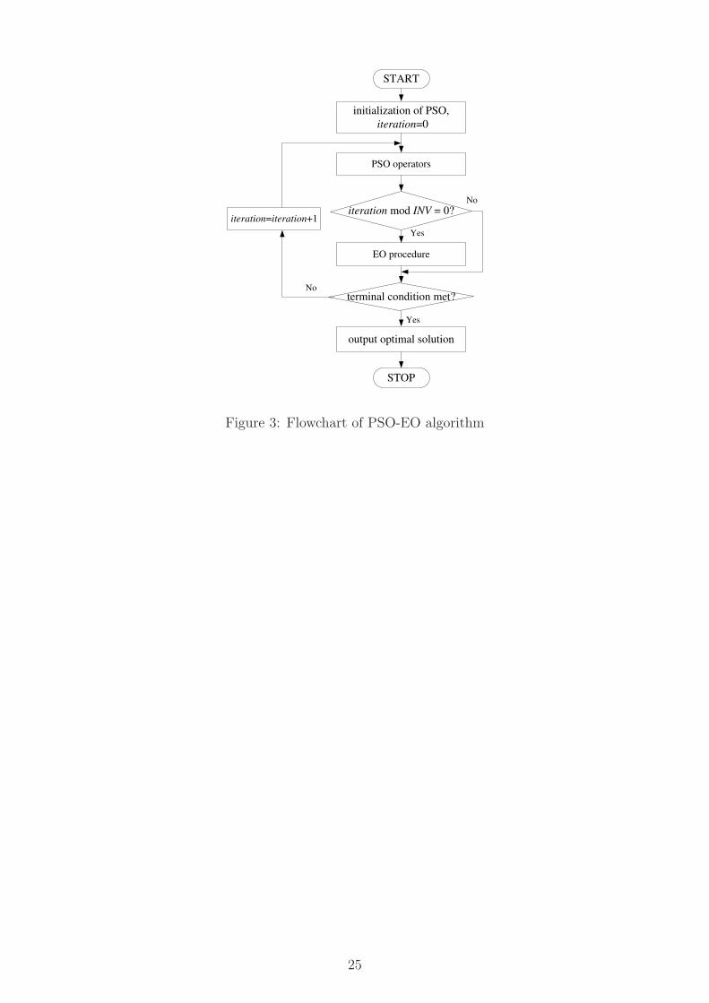
For a minimization problem with D dimensions, the hybrid PSO-EO algorithm works as Figure

2 and its flowchart is illustrated in Figure 3. In the main procedure of PSO-EO algorithm, the

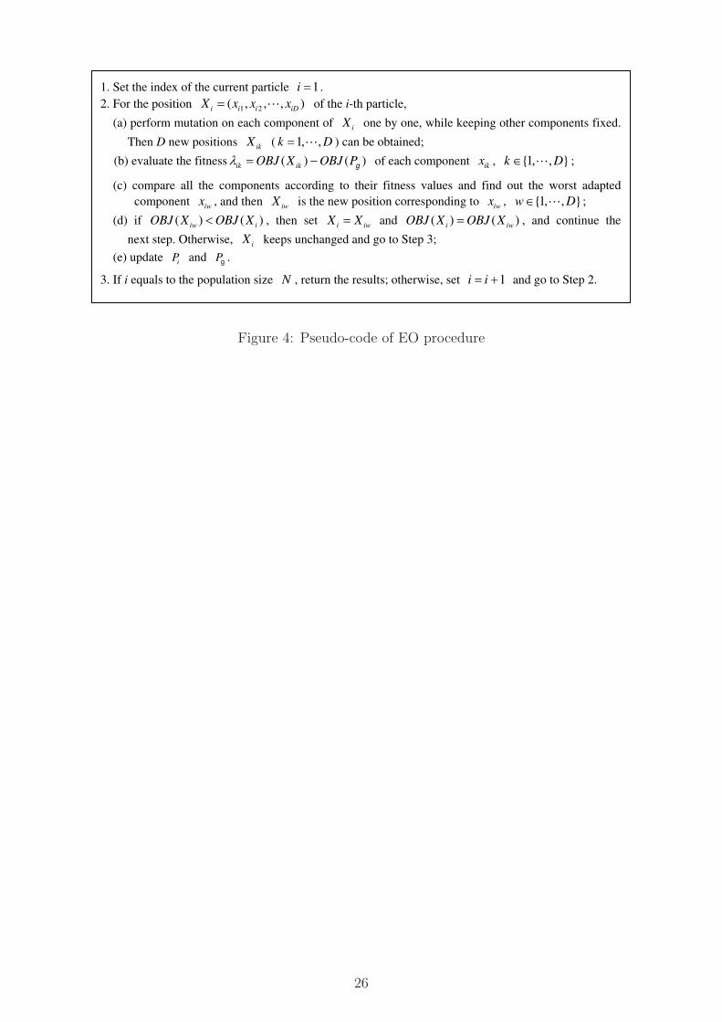
fitness of each particle is evaluated through putting its position into the objective function.

However, in the EO procedure, in order to find out the worst component, each component of

a solution should be assigned a fitness value. We define the fitness of each component of a

solution for an unconstrained minimization problem as follows. For the i-th particle, the fitness

λik of the k-th component is defined as the mutation cost, i.e. OBJ(Xik) − OBJ(Pg), where

Xik is the new position of the i-th particle obtained by performing mutation only on the k-th

component and leaving all other components fixed, OBJ(Xik) is the objective value of Xik,

and OBJ(Pg) is the objective value of the best position in the swarm found so far. The EO

procedure is described in Figure 4.

3.2 Mutation Operator

Since there is merely mutation operator in EO, the mutation plays a key role in EO search.

In this work, we adopt the hybrid GC mutation operator presented by Chen and Lu [34].

This mutation method mixes Gaussian mutation and Cauchy mutation. The mechanisms of

Gaussian and Cauchy mutation operations have been studied by Yao et al. [38]. They pointed

out that Cauchy mutation is better at coarse-grained search while Gaussian mutation is better

at fine-grained search. In the hybrid GC mutation, the Cauchy mutation is first used. It means

that the large step size will be taken first at each mutation. If the new generated variable after

mutation goes beyond the range of variable, the Cauchy mutation will be used repeatedly for

5

some times (TC), until the new generated offspring falls into the range. Otherwise, Gaussian

mutation will be carried out repeatedly for another some times (TG), until the offspring satisfies

the requirement. That is, the step size will become smaller than before. If the new generated

variable after mutation still goes beyond the range of variable, then the upper or lower bound

of the decision variable will be chosen as the new generated variable. Thus, the hybrid GC

mutation combines the advantages of coarse-grained search and fine-grained search. Unlike

some switching algorithms which have to decide when to switch between different mutations

during search, the hybrid GC mutation does not need to make such decisions.

In this study, the Gaussian mutation performs with the following representation:

x′k = xk + Nk(0, 1) (3)

where xk and x′k denote the k-th decision variables before mutation and after mutation, respec-

tively, Nk(0, 1) denotes the Gaussian random number with mean zero and standard deviation

one and is generated anew for k-th decision variable. The Cauchy mutation performs as follows:

x′k = xk + δk (4)

where δk denotes the Cauchy random variable with the scale parameter equal to one and is

generated anew for the k-th decision variable.

In the hybrid GC mutation, the values of parameters TC and TG are set by the user

beforehand. The value of TC decides the coarse-grained searching time, while the value of TG

has an effect on the fine-grained searching time. Therefore, both values of the two parameters

can not be large because it will prolong the search process and hence increase the computational

overhead. According to the literature [34], the moderate values of TC and TG can be set to

2∼4.

4 Experiments and Results

4.1 Test Functions

In order to demonstrate the performance of the proposed hybrid PSO-EO, we use six well-

known benchmark functions shown in Table 1 . All the functions are to be minimized. For

these functions, there are many local optima and/or saddles in their solution spaces. The

amount of local optima and saddles increases with increasing complexity of the functions, i.e.

with increasing dimension.

6

4.2 Experimental Settings

To testify the efficiency and effectiveness of the the proposed approach, the experimental results

of the proposed approach are compared with those of standard PSO, PEO and standard GA.

Note that all the algorithms were run on the same hardware (i.e., Intel Pentium M with

900 MHz CPU and 256M memory) and software (i.e., JAVA) platform. Each algorithm was

run independently for 20 trials. Table 2 shows the settings of problem dimension, maximum

generation, population size, initialization range of each algorithm, and the value of parameter

INV for each test function.

For the hybrid PSO-EO, the cognitive and social scaling parameters, i.e. c1 and c2, were

both set to 2, the inertia weight w varied from 0.9 to 0.4 linearly with the iterations, the upper

and lower bounds for velocity on each dimension, i.e., (vmin, vmax), were set to be the upper

and lower bounds of each dimension, i.e. (vmin, vmax) = (xmin, xmax). The parameters TC and

TG in the hybrid GC mutation were both set to 3. From the values of parameter INV shown

in Table 2 , we can see that EO was introduced to PSO more frequently on functions f1, f2 and

f6 than other three functions due to the complexity of problems. For the standard PSO, all

the parameters, i.e., c1, c2, w and (vmin, vmax), were set to the same as those used in the hybrid

PSO-EO. For the PEO, we also adopted the hybrid GC mutation with both parameters TC

and TG equal to 3. For the standard GA, we used elitism mechanism, roulette wheel selection

mechanism, single-point uniform crossover with the rate of 0.3, non-uniform mutation with the

rate of 0.05 and the system parameter of 0.1.

In order to compare the different algorithms, a fair time measure must be selected. The

number of iterations cannot be used as a time measure, as these algorithms do different amounts

of work in their inner loops. It is also noticed that each component of a solution in the EO

procedure has to be evaluated each iteration, and thus the calculation of the number of function

evaluations will bring some trouble. Therefore, the number of function evaluations is not very

suitable as a time measure. In this work, we adopt the average runtime of twenty runs when

the near-optimal solution is found or otherwise when the maximum generation is reached as a

time measure.

4.3 Simulation Results and Discussions

After 20 trials of running each algorithm for each test function, the simulation results were

obtained and shown in Tables 3∼8 . Denote F as the result found by the algorithms and F ∗ as

the optimum value of the functions. The simulation is considered successful, or in other words,

7

the near-optimal solution is found, if F satisfies that |(F ∗ − F )/F ∗| < 1E − 3 (for the case

F ∗ 6= 0) or |F ∗ − F | < 1E − 3 (for the case F ∗ = 0). In these tables, “Success” represents the

successful rate, and “Runtime” is the average runtime of twenty runs when the near-optimal

solution is found or otherwise when the maximum generation is reached. The worst, mean,

best and standard deviation of solutions found by the four algorithms are also listed in these

tables. Note that the standard deviation of solutions indicates the stability of the algorithms,

and the successful rate represents the robustness of the algorithms.

The Michalewicz function is a highly multimodal test function (with n! local optima). The

parameter m defines the “steepness” of the valleys or edges. Larger m leads to more difficult

search. For very large m, the function behaves like a needle in the haystack (the function values

for points in the space outside the narrow peaks give very little information on the location of

the global optimum) [39]. As can be seen from Table 3, PSO-EO significantly outperformed

PSO, PEO and GA in terms of solution quality, convergence speed and successful rate. It is

interesting to notice that PSO-EO converged to the global optimum about 40 times faster than

the other three algorithms on this function.

With regard to the Schwefel function, its surface is composed of a great number of peaks

and valleys. The function has a second best minimum far from the global minimum where

many search algorithms are trapped. Moreover, the global minimum is near the bounds of the

domain. The search algorithms are potentially prone to convergence in the wrong direction in

optimization of this function [39]. Consequently, this function is very hard to solve for many

state-of-the-art optimization algorithms. Nevertheless, PSO-EO showed its great search ability

and the prominent capability of escaping from local optima when dealing with this function.

From Table 4, it is clear that PSO-EO was still the winner which was capable of converging

to the global optimum with 100% successful rate, whereas the other three algorithms were not

able to find the global optimum at all. It is important to point out that, in order to help the

PSO to jump out of local optima, the EO procedure was introduced to PSO each iteration.

Thus, the exploitation search played a critical role in optimization of the Schwefel function.

The Griewank function is a highly multimodal function with many local minima distributed

regularly [40]. The difficult part about finding the optimal solution to this function is that an

optimization algorithm easily can be trapped in a local optimum on its way towards the global

optimum. From Table 5 , we can see that PSO-EO, PSO and PEO could find the global

optimum with 100% successful rate. However, PSO-EO converged to the optimal solution

more quickly than PSO and PEO, and found more accurate solution than PEO.

8

Table 6 and Table 7 show the simulation results of each algorithm on the functions Rastrigin

and Ackley, respectively. Both of the two functions are highly multimodal and their patterns

are similar to that observed with Griewank function. As can be seen from Table 6 and Table

7, only PSO-EO and PSO were capable of finding the global optimum on the two functions,

but PSO-EO performed better than PSO with respect to convergence speed.

Note that the EO procedure was introduced to PSO every 100 iterations in optimization of

functions Griewank, Rastrigin and Ackley. In other words, PSO played a key role in optimiza-

tion of these functions, while EO brought the diversity to the solutions generated by PSO at

intervals. In this way, the hybrid PSO-EO algorithm is able to preserve the fast convergence

ability of PSO.

The Rosenbrock function is a unimodal optimization problem. Its global optimum is inside

a long, narrow, parabolic shaped flat valley, popularly known as the Rosenbrock’s valley [39].

It is trivial to find the valley, but it is a difficult task to achieve convergence to the global

optimum. The Rosenbrock function proves to be hard to solve for all the algorithms, as can be

observed from Table 8. On this function, only PSO-EO could find the global optimum. Due to

the difficulty in finding the global optimum of this function, the EO procedure was introduced

to PSO each iteration.

In a general analysis of the simulation results shown in Table 3∼ Table 8, the following

conclusions can be drawn:

• On the convergence speed, PSO-EO was the fastest algorithm in comparison with the

other three algorithms for all the functions. Thus, the hybrid PSO-EO can be considered

a very fast algorithm when solving numerical optimization problems, especially those

complex multimodal functions.

• With respect to the stability of algorithms, PSO-EO showed the best stability as com-

pared to PSO, PEO and GA. The standard deviations of solutions found by PSO-EO on

functions f1, f2 and f6 were the smallest among all the algorithms, and as good as those

found by PSO on functions f3, f4 and f5. Overall, PSO-EO is a highly stable algorithm

that is capable of obtaining reasonable consistent results.

• In terms of the robustness of algorithms, PSO-EO significantly outperformed the other

three algorithms. PSO-EO was capable of finding the global optimum with 100% suc-

cessful rate on all the test functions, especially on functions Schwefel and Rosenbrock,

which are very difficult to solve for many state-of-the-art optimization algorithms. Hence,

PSO-EO can be regarded as a highly robust optimization algorithm.

9

• PSO-EO showed its strong capability of escaping from local optima when dealing with

those highly multimodal functions, e.g. functions Michalewicz and Schwefel. PSO-EO

also exhibited its great search ability when handling those unimodal functions which are

hard to solve for many optimization problems, e.g. Rosenbrock function.

• In this study, the dimensions of all the test functions are 30, except for the Michalewicz

function with the dimension of 10. It is observed that PSO-EO performs well in opti-

mization of those functions with high dimension. This suggests that PSO-EO is very

suitable for thoes functions with high dimension.

• The value of parameter INV determines the frequency of introducing the EO procedure to

PSO. As a consequence, the hybrid PSO-EO algorithm elegantly combines the exploration

ability of PSO with the exploitation ability of EO via tuning the parameter INV . This

offers the explanation as to the better performance of the hybrid PSO-EO algorithm in

comparison with standard PSO, PEO and standard GA.

From the above summary, it can be concluded that the proposed approach possesses superior

performance in accuracy, convergence speed, stability and robustness, as compared to standard

PSO, PEO and standard GA. As a result, our approach is a perfectly good performer in

optimization of those complex high-dimensional functions.

5 Conclusion and Future Work

In this paper, we have developed a novel hybrid optimization method, called hybrid PSO-EO

algorithm, through introducing EO to PSO. The hybrid approach combines the exploration

ability of PSO with the exploitation ability of EO, and thus has strong capability of pre-

venting premature convergence. Compared with standard PSO, PEO and standard GA with

six well-known benchmark functions, it has been shown that our approach possesses superior

performance in accuracy, convergence rate, stability and robustness. The simulation results

demonstrate that PSO-EO is well suited to those complex unimodal/multimodal functions

with high dimension. As a consequence, PSO-EO may be a promising and viable tool to deal

with complex numerical optimization problems. The future work includes the studies on how

to extend PSO-EO to handle multiobjective optimization problems. It is desirable to further

apply PSO-EO to solving those more complex real-world optimization problems.

10

Acknowledgments

This work is supported by the National Natural Science Foundation of China under Grant No.

60772148.

References

[1] J. Kennedy, R.C. Eberhart, Particle swarm optimization. Proceedings of the 1995 IEEE Interna-

tional Conference on Neural Networks, IEEE Service Center, Piscat away, 1995, pp. 1942-1948.

[2] R.C. Eberhart, J. Kennedy, A New Optimizer Using Particle Swarm Theory. Proceedings of the

Sixth International Symposium on Micromachine and Human Science, Nagoya, Japan, 1995, pp.

39-43.

[3] P. J. Angeline, Using selection to improve particle swarm optimization. Proceedings of the IEEE

Congress on Evolutionary Computation, Anchorage, Alaska, USA, 1998, pp. 84-89.

[4] M. Løvbjerg, T. K. Rasmussen, T. Krink, Hybrid particle swarm optimiser with breeding and

subpopulations. Proceedings of the Genetic and Evolutionary Computation Conference, San

Francisco, Morgan Kaufmann Publishers, 2001, pp. 469-476.

[5] K. E. Parsopoulos, V. P. Plagianakos, G. D. Magoulas, M. N. Vrahatis, Stretching technique for

obtaining global minimizers through particle swarm optimization. Proceedings of the Workshop

on Particle Swarm Optimization, Indianapolis, IN, 2001, pp. 22-29.

[6] K. E. Parsopoulos, M. N. Vrahatis, Initializing the particle swarm optimizer using the nonlinear

simplex Method. Advances in Intelligent Systems, Fuzzy Systems, Evolutionary Computation,

WSEAS Press,2002, pp.216-221.

[7] N. Higashi, H. Iba, Particle swarm optimization with gaussian mutation. Proceedings of the

IEEE Swarm Intelligence Symposium 2003, Indianapolis, Indiana, USA, 2003, pp. 72-79.

[8] X. H. Shi, Y.H. Lu, C.G. Zhou, H.P. Lee, W.Z. Lin, Y.C. Liang, Hybrid evolutionary algorithms

based on PSO and GA. Proceedings of IEEE Congress on Evolutionary Computation 2003,

Canbella, Australia, 2003, pp. 2393-2399.

[9] S. K. S. Fan, E. Zahara, A hybrid simplex search and particle swarm optimization for uncon-

strained optimization. European Journal of Operational Research 181(2007)527-548.

[10] Y. Jin, K. Joshua, H. Lu, Y. Liang, B. K. Douglas, The landscape adaptive particle swarm

optimizer, Applied Soft Computing 8(2008) 295-304.

[11] Hongbo Liu, Ajith Abraham, Maurice Clerc,Chaotic dynamic characteristics in swarm intelli-

gence,Applied Soft Computing 7 (2007)1019-1026

11

[12] DeBao Chen, ChunXia Zhao,Particle swarm optimization with adaptive population size and its

application,Applied Soft Computing (2008), doi:10.1016/j.asoc.2008.03.001

[13] M. Senthil Arumugam, M.V.C. Rao, Alan W.C. Tan, A Novel and Effective Particle Swarm

Optimization like Algorithm with Extrapolation Technique,Applied Soft Computing (2008),

doi:10.1016/j.asoc.2008.04.016.

[14] Yi-Tung Kao, Erwie Zahara,A hybrid genetic algorithm and particle swarm optimization for

multimodal functions,Applied Soft Computing 8(2008)849-857.

[15] M. Senthil Arumugam, M.V.C. Rao,On the improved performances of the particle swarm opti-

mization algorithms with adaptive parameters, cross-over operators and root mean square (RMS)

variants for computing optimal control of a class of hybrid systems, Applied Soft Computing 8

(2008) 324-336.

[16] Y. Jiang, T. Hu, C. Huang, X. Wu, An improved particle swarm optimization algorithm.Applied

Mathematics and Computation 193(2007) 231-239.

[17] R. Brits, A.P. Engelbrecht, F. van den Bergh, Locating multiple optima using particle swarm

optimization. Applied Mathematics and Computation 189(2007)1859-1883.

[18] P.S. Shelokar, Patrick Siarry, V.K. Jayaraman, B.D. Kulkarni, Particle swarm and ant colony

algorithms hybridized for improved continuous optimization. Applied Mathematics and Compu-

tation 188 (2007)129-142.

[19] T. Xiang, K. Wong, X. Liao, A novel particle swarm optimizer with time-delay. Applied Mathe-

matics and Computation 186(2007) 789-793.

[20] T. Xiang, X. Liao, K. Wong, An improved particle swarm optimization algorithm combined with

piecewise linear chaotic map. Applied Mathematics and Computation 190(2007) 1637-1645.

[21] B. Niu, Y. Zhu, X. He, H. Wu, MCPSO: A multi-swarm cooperative particle swarm optimizer.

Applied Mathematics and Computation 185(2007) 1050-1062.

[22] X. Yang, J. Yuan, J. Yuan, H. Mao, A modified particle swarm optimizer with dynamic adapta-

tion. Applied Mathematics and Computation 189(2007)1205-1213.

[23] S. Boettcher, A. G. Percus, Extremal optimization: methods derived from co-evolution. Pro-

ceedings of the genetic and evolutionary computation conference,1999, pp. 825-832.

[24] S. Boettcher, A. G. Percus, Nature’s way of optimizing. Artificial Intelligence 119(2000) 275-286.

[25] P. Bak, K. Sneppen, Punctuated equilibrium and criticality in a simple model of evolution.

Physical Review Letters 71(1993)4083-4086.

[26] P. Bak, C Tang, K. Wiesenfeld, Self-organized criticality. Physical Review Letters 59(1987)381-

384.

[27] S. Boettcher, A.G. Percus, Optimizing glasses with extremal dynamics. Computer Simulation

Studies in Condensed-Matter Physics XVI,Springer Berlin Heidelberg,Part II, 2006, pp.74-79.

12

[28] S. Boettcher, A.G. Percus, Extremal optimization at the phase transition of the 3-coloring prob-

lem. Physical Review E 69(2004) 066703.

[29] Yong-Zai Lu, Min-Rong Chen, Yu-Wang Chen, Studies on extremal optimization and its appli-

cations in solving real world optimization problems. Proceedings of the 2007 IEEE Symposium

on Foundations of Computational Intelligence (FOCI 2007), Hawaii, USA, 2007, pp.162-168.

[30] Yu-Wang Chen, Yong-Zai Lu, Genke Yang, Hybrid evolutionary algorithm with marriage of

genetic algorithm and extremal optimization for production scheduling. International Journal of

Advanced Manufacturing Technology 36(2008)959-968.

[31] Yu-Wang Chen, Yong-Zai Lu, Genke Yang, Optimization with extremal dynamics for the trav-

eling salesman problem. Physica A 385(2007)115-123.

[32] Min-Rong Chen, Yong-Zai Lu, Genke Yang, Multiobjective extremal optimization with applica-

tions to engineering design, Journal of Zhejiang University-SCIENCE A 8(2007)1905-1911.

[33] Min-Rong Chen, Yong-Zai Lu, Genke Yang, Multiobjective optimization using population-based

extremal optimization, Journal of Neural Computing and Applications 7(2008)101-109.

[34] Min-Rong Chen, Yong-Zai Lu,A novel elitist multiobjective optimization algorithm: multiobjec-

tive extremal optimization. European Journal of Operational Research 188(2008)637-651.

[35] I. Moser, T. Hendtlass, Solving problems with hidden dynamics-comparison of extremal optimiza-

tion and ant colony system. Proceedings of 2006 IEEE Congress on Evolutionary Computation

(CEC’2006), 2006, pp. 1248-1255.

[36] Min-Rong Chen, Yong-Zai Lu, Genke Yang, Population-based extremal optimization with adap-

tive Levy mutation for constrained optimization. Proceedings of 2006 International Conference

on Computational Intelligence and Security (CIS’06), 2006,pp. 258-261.

[37] S. Boettcher, A. G. Percus, Optimization with extremal dynamics.Physical Review Letters

86(2001) 5211-5214 .

[38] X. Yao, Y. Liu, G. Lin, Evolutionary programming made faster. IEEE Transactions on Evolu-

tionary Computation 3(1999) 82-102.

[39] M. Molga,C. Smutnicki,Test functions for optimization needs. Available at

http://www.zsd.ict.pwr.wroc.pl/files/docs/functions.pdf, 2005.

[40] D. Srinivasan, T. H. Seow,Particle swarm inspired evolutionary algorithm (PS-EA) for multi-

criteria optimization problems. Evolutionary Multiobjective Optimization, Springer Berlin Hei-

delberg, 2006, pp.147-165.

13

Table 1: Test functions

Table 2: Parameter settings for six test functions

Table 3: Comparison results for Michalewicz function f1 (F ∗1 = −9.66)

Table 4: Comparison results for Schwefel function f2 (F ∗2 = −12569.5)

Table 5: Comparison results for Griewank function f3 (F ∗3 = 0)

Table 6: Comparison results for Rastrigin function f4 (F ∗4 = 0)

Table 7: Comparison results for Ackley function f5 (F ∗5 = 0)

Table 8: Comparison results for Rosenbrock function f6 (F ∗6 = 0)

Figure 1: Pseudo-code of EO algorithm

Figure 2: Pseudo-code of PSO-EO algorithm

Figure 3: Flowchart of PSO-EO algorithm

Figure 4: Pseudo-code of EO procedure

14

Table 1: Test functionsFunction Function expression Search space Global minimum

Michalewicz f1(X) = −∑ni=1 sin (xi) sin2m(

i−x2i

π), m = 10 (0, π)n -9.66

Schwefel f2(X) = −∑ni=1(xi sin(

√|xi|)) (−500, 500)n -12569.5

Griewank f3(X) = 14000

∑ni=1 x2

i −∏n

i=1 cos( xi√i) + 1 (−600, 600)n 0

Rastrigin f4(X) =∑n

i=1[x2i − 10 cos (2πxi) + 10] (−5.12, 5.12)n 0

Ackley f5(X) = 20 + e− 20e[−0.2√

1n

∑ni=1 x2

i ] − e1n

∑ni=1 cos(2πxi) (−32.768, 32.768)n 0

Rosenbrock f6(X) =∑n−1

i=1 [100(xi+1 − x2i )

2 + (xi − 1)2] (−30, 30)n 0

15

Table 2: Parameter settings for six test functions

Function Dimension Maximum generation Population size Initialization range INV

f1 10 20000 10 (0, π)n 20

f2 30 20000 30 (−500, 500)n 1

f3 30 20000 30 (−600, 600)n 100

f4 30 20000 10 (−5.12, 5.12)n 100

f5 30 10000 30 (−32.768, 32.768)n 100

f6 30 100000 30 (−30, 30)n 1

16

Table 3: Comparison results for Michalewicz function f1 (F ∗1 = −9.66)

Algorithm Runtime(s) Success(%) Worst Mean Best St.Dev.

PSO-EO 3.5 100 -9.66 -9.66 -9.66 1.58E-3

PSO 134.4 5 -9.06 -9.52 -9.66 0.15

PEO 169.8 0 -9.50 -9.55 -9.60 0.03

GA 118.6 60 -9.49 -9.63 -9.66 0.05

17

Table 4: Comparison results for Schwefel function f2 (F ∗2 = −12569.5)

Algorithm Runtime(s) Success(%) Worst Mean Best St.Dev.

PSO-EO 301.7 100 -12569.5 -12569.5 -12569.5 0.0

PSO 400.5 0 -7869.3 -8868.4 -10130.5 791.48

PEO 644.9 0 -12214.2 -12297.1 -12451.1 112.36

GA 400.9 0 -8285.9 -8906.9 -9253.0 582.35

18

Table 5: Comparison results for Griewank function f3 (F ∗3 = 0)

Algorithm Runtime(s) Success(%) Worst Mean Best St.Dev.

PSO-EO 0.91 100 0.0 0.0 0.0 0.0

PSO 0.96 100 0.0 0.0 0.0 0.0

PEO 34.0 100 6.56E-4 5.43E-4 4.78E-4 5.48E-05

GA 219.2 0 0.069 0.047 0.006 0.02

19

Table 6: Comparison results for Rastrigin function f4 (F ∗4 = 0)

Algorithm Runtime(s) Success(%) Worst Mean Best St.Dev.

PSO-EO 0.9 100 0.0 0.0 0.0 0.0

PSO 1.4 100 0.0 0.0 0.0 0.0

PEO 197.0 0 2.64 2.16 1.73 0.30

GA 173.7 0 0.019 0.008 0.002 5.6E-3

20

Table 7: Comparison results for Ackley function f5 (F ∗5 = 0)

Algorithm Runtime(s) Success(%) Worst Mean Best St.Dev.

PSO-EO 0.57 100 0.0 0.0 0.0 0.0

PSO 1.14 100 0.0 0.0 0.0 0.0

PEO 248.7 0 0.12 0.11 0.10 6.0E-3

GA 120.6 0 0.096 0.061 0.030 0.02

21

Table 8: Comparison results for Rosenbrock function f6 (F ∗6 = 0)

Algorithm Runtime(s) Success(%) Worst Mean Best St.Dev.

PSO-EO 314.8 100 9.54E-4 9.90E-4 9.99E-4 1.31E-5

PSO 389.8 0 27.4 26.19 24.10 1.31

PEO 1224.9 0 8.53 7.63 5.85 0.92

GA 525.6 0 31.69 29.17 22.11 3.97

22

1. Randomly generate a solution 1 2( , , , )DX x x x . Set optimal solution bestX X and the

minimum cost function .( ) (bestC X C X )

2. For the current solution X ,

(a) evaluate the fitness i for each variable ix , {1,2, }i D ,

(b) rank all the fitnesses and find the variable jx with the lowest fitness, i.e., j i for all ,i

(c) choose one solution 'X in the neighborhood of X , such that the j-th variable must change its

state,

(d) accept 'X X unconditionally,

(e) if then set ( ) ( )bestC X C X bestX X and C X( ) (best )C X .

3. Repeat Step 2 as long as desired.

4. Return bestX and C X .( )best

Figure 1: Pseudo-code of EO algorithm

23

1. Initialize a swarm of particles with random positions and velocities on dimensions. N D

Set .= 0iteration

2. Evaluate the fitness value of each particle, and update ( i Ni

P 1, , ) and .Pg

3. Update the velocity and position of each particle using Eq.1 and Eq.2, respectively.

4. Evaluate the fitness value of each particle, and update ( i Ni

P 1, ,

0

) and .Pg

5. If , the EO procedure is introduced. Otherwise, continue the next step. ( mod )iteration INV

6. If the terminal condition is satisfied, go to the next step; otherwise, set = 1iteration iteration ,

and go to Step 3.

7.Output the optimal solution and the optimal objective function value.

Figure 2: Pseudo-code of PSO-EO algorithm

24

Noterminal condition met?

output optimal solution

STOP

Yes

initialization of PSO,

iteration=0

START

PSO operators

EO procedure

Yes

iteration mod INV = 0?iteration=iteration+1

No

Figure 3: Flowchart of PSO-EO algorithm

25

1. Set the index of the current particle 1i .

2. For the position 1 2( , , , )i i i iD

X x x x of the i-th particle,

(a) perform mutation on each component of i

X one by one, while keeping other components fixed.

Then D new positions ik

X ( k ) can be obtained; 1, , D

)(b) evaluate the fitness ( ) (ik ik

OBJ X OBJ Pg

of each component ik

x , ;{1, , }k D

(c) compare all the components according to their fitness values and find out the worst adapted

component iw

x , and then iw

X is the new position corresponding to iw

x , ;{1, , }w D

(d) if , then set ( ) (iw i

OBJ X OBJ X )iwi

X X and ( ) (i

OBJ X OBJ X )iw

, and continue the

next step. Otherwise, i

X keeps unchanged and go to Step 3;

(e) update and .i

P Pg

3. If i equals to the population size N , return the results; otherwise, set 1i i and go to Step 2.

Figure 4: Pseudo-code of EO procedure

26