Southern Methodist University Southern Methodist University

SMU Scholar SMU Scholar

Electrical Engineering Theses and Dissertations Electrical Engineering

Fall 12-2018

A Novel Ultrasound Imaging Technique Using Random Signals A Novel Ultrasound Imaging Technique Using Random Signals

Anahita Khalilzadeh Southern Methodist University, anahita.khalilzadeh@gmail.com

Follow this and additional works at: https://scholar.smu.edu/engineering_electrical_etds

Part of the Electrical and Electronics Commons

Recommended Citation Recommended Citation Khalilzadeh, Anahita, "A Novel Ultrasound Imaging Technique Using Random Signals" (2018). Electrical Engineering Theses and Dissertations. 16. https://scholar.smu.edu/engineering_electrical_etds/16

This Thesis is brought to you for free and open access by the Electrical Engineering at SMU Scholar. It has been accepted for inclusion in Electrical Engineering Theses and Dissertations by an authorized administrator of SMU Scholar. For more information, please visit http://digitalrepository.smu.edu.

A NOVEL ULTRASOUND IMAGING TECHNIQUE

USING RANDOM SIGNALS

Approved by:

_______________________________________

Prof. Carlos Davila

Associate Professor of Electrical Engineering

___________________________________

Prof. James Dunham

Associate Professor of Electrical Engineering

___________________________________

Prof. Behrouz Peikari

Professor of Electrical Engineering

A NOVEL ULTRASOUND IMAGING TECHNIQUE

USING RANDOM SIGNALS

A Thesis Presented to the Graduate Faculty of

Lyle school of Engineering

Southern Methodist University

in

Partial Fulfillment of the Requirements

for the degree of

Master of Science in Electrical Engineering

by

Anahita Khalilzadeh

B.Sc., Electrical Engineering, Sharif University of Technology, Tehran, Iran

Dec 15, 2018

Copyright (2018)

Anahita Khalilzadeh

All Rights Reserved

iv

ACKNOWLEDGMENTS

I would like to thank Prof. Davila for his insightful comments and enlightening

discussions.

v

Khalilzadeh, Anahita B.Sc., Electrical Engineering, Sharif University of Technology,

Tehran, 2015

A Novel Ultrasound Imaging Technique

Using Random Signals

Advisor: Professor Carlos Davila

Master of Science conferred Dec 15, 2018

Dissertation completed Nov 15, 2018

Ultrasound imaging has been used extensively because of its benign nature and relatively

low cost implementation. The most common approach for forming an image is Brightness Mode

(B-Mode), which uses an array with dynamic focusing. Focus is performed through Phase

Shifters that are bulky and complicated components which increases the device cost.

This research describes a new method to form an Ultrasound image, without relying on

phase shifting. The proposed method offers a lower cost solution compared to the B-Mode

systems and overcomes some of their inherent limitations.

vi

TABLE OF CONTENTS

LIST OF FIGURES ................................................................................................................. viii

CHAPTER 1: Introduction ......................................................................................................... 1

1.1 Ultrasound wave propagation ....................................................................................... 1

1.2 Acoustic wave transducers ........................................................................................... 3

1.3 Scattering Field Calculation ......................................................................................... 6

CHAPTER 2: Overview of Ultrasonic Imaging Systems ........................................................... 7

2.1 A-Mode ......................................................................................................................... 7

2.2 B-Mode ......................................................................................................................... 9

2.3 C-Mode ....................................................................................................................... 11

2.4 Other ultrasonic imaging systems............................................................................... 12

CHAPTER 3: Proposed Methodology ...................................................................................... 13

3.1 Unfocused array .......................................................................................................... 13

3.2 Proposed method ........................................................................................................ 14

3.3 Practical implementation ............................................................................................ 22

3.4 Proposed system block diagram ................................................................................. 24

CHAPTER 4: Experimental Results ......................................................................................... 29

4.1 Scattering value result along a circular path ............................................................... 29

4.2 Full 2D image ............................................................................................................. 30

vii

4.3 Performance in presence of imperfections ................................................................. 31

4.4 Implementation with binary coefficients .................................................................... 33

CHAPTER 5: Summary and Conclusions ................................................................................ 34

5.1 Future work................................................................................................................. 34

viii

LIST OF FIGURES

Figure 1. An arbitrarily shaped transducer in the coordinates system. ........................................... 4

Figure 2. An A-mode ultrasonic imaging system. .......................................................................... 7

Figure 3. Received echo pulse field for an A-mode system with two objects located 30 mm apart.

Excitation is a single 3 MHz sinusoidal pulse. ............................................................................... 8

Figure 4. B-mode imaging using an array. ..................................................................................... 9

Figure 5. Simple two element phase array. ................................................................................... 10

Figure 6. A simple C-mode imaging system. ............................................................................... 12

Figure 7. Two equal distance objects in far field of an unfocused array. ..................................... 13

Figure 8. Single element in far field. ............................................................................................ 14

Figure 9. Array pressure calculation on circle. ............................................................................. 16

Figure 10. Pressure of an array with 100 elements and spacing of 𝜆/15. (a): Non-zero average

pressures (b): Zero average pressure............................................................................................. 19

Figure 11. Active-set Algorithm flowchart. .................................................................................. 21

Figure 12. Forming an image with proposed system. ................................................................... 23

Figure 13. Pressure variability with spacing, N=100, and M varied from 100 to 500. ................ 24

Figure 14. A full digital implementation of TX. ........................................................................... 25

Figure 15 An analog implementation of TX. ................................................................................ 27

Figure 16 One dimensional image of a single scatterer at 𝑥 = −20 𝑚𝑚 on a circular path with

𝑟𝑐𝑖𝑟𝑐 = 115 𝑚𝑚. ......................................................................................................................... 29

ix

Figure 17. One dimensional image of two scatterers at 𝑥 = −20 𝑚𝑚 and 𝑥 = 10 𝑚𝑚 on a

circular path with 𝑟𝑐𝑖𝑟𝑐 = 115 𝑚𝑚. ............................................................................................ 30

Figure 18. 2D image. Left the original scatterers location, right captured image. ....................... 31

Figure 19. Noise sensitivity of scatterer detection (a) SNR=20 dB (b) SNR=0 dB ..................... 31

Figure 20. Sensitivity of scatterer detection to 20% rms gain and phase error ............................ 33

Figure 21 Image of two scatterers at 𝑥 = −20 𝑚𝑚 and 𝑥 = 10 𝑚𝑚 on a circular path with

𝑟𝑐𝑖𝑟𝑐 = 115𝑚𝑚 with binary TX coefficients. ............................................................................. 33

To my parents, who have been always there for me.

1

CHAPTER 1

Introduction

Ultrasonic imaging has been widely used as a safe, accurate, and low-cost diagnosis

technique. Being of acoustic nature, ultrasound waves range from frequencies above the human

hearing range (i.e. 20 KHz) to several hundreds of MHz. In this chapter we present an overview

of the basics of ultrasound wave propagation, generation, and scattering from the literature. This

provides an understanding of the ultrasound imaging underlying physics.

1.1 Ultrasound wave propagation

The wave propagates by changing the pressure and vibrating the molecules in a medium and,

therefore, we have to study the air/medium pressure. This derivation follows [1] and [2]. The

pressure and speed of a medium follow the relationship:

−𝜕𝑝

𝜕𝑧= 𝜌 (

𝜕𝑢

𝜕𝑡+ 𝑢

𝜕𝑢

𝜕𝑧) (1)

where 𝑝 and 𝑢 denote the pressure and speed, and 𝑧 and 𝑡 are the propagation direction and time,

respectively.

By applying the conservation of mass principle and incorporating the coefficient 𝐾 which

quantifies the compressibility under a pressure field, assuming no heat conduction or conversion

exists, we can write

𝜕𝑝

𝜕𝑡+

1

𝐾

𝜕𝑢

𝜕𝑧= 0 (2)

2

By taking partially derivatives the wave equation for acoustic wave is obtained.

𝜕2𝑝

𝜕𝑧2− ρ0𝐾

𝜕2𝑝

𝜕𝑡2= 0. (3)

This is a Helmholtz equation similar to the equation governing electromagnetic waves [3] and has

similar solutions. It should be noted that the spatial differentiation is in fact the Laplacian operator

∇2 which has been simplified into a single dimension derivative under the assumption that wave

is propagating in this direction. A more general form of wave propagation that has been given in

many prior works [2, 4, 5] which is applicable to the case where the media is nonhomogeneous is

∇2𝑝 − 𝜌0𝐾𝜕2𝑝

𝜕𝑡2=

1

𝜌∇𝜌. ∇𝑝. (4)

Here ρ0 is the average medium density that undergoes a perturbation due to the pressure field

which the “. ” operation represents the vector inner product operation. 𝜌 denotes the medium

density as a function of time and location. The right hand of this equation falls to zero in

homogenous media and it can be simplified to Equation (3).

The solution to the wave propagation equation in a homogenous media assuming that the wave is

propagating along 𝑧 axis is

𝑝 = 𝑝+𝑐𝑜𝑠(ω𝑡 − 𝑘𝑧 + ϕ+) + 𝑝−𝑐𝑜𝑠(ω𝑡 + 𝑘𝑧 + ϕ−) (5)

which consists of two responses that are propagating in opposite directions. By plugging this

solution into Equation (4) it can be seen that the constant 𝑘 is determined by the properties of

material (𝐾,ρ, and 𝜌0) and the wave frequency ω according to Equation (3).

And so

𝑘2 = 𝐾ρω2 (6)

3

where the parameter 𝑘 is closely related to the wavelength, as it can be readily seen, and 𝑘 =2π

λ.

Similarly wave speed can be calculated to be

𝑐 =1

√(ρ0𝐾) . (7)

Interestingly, almost all our knowledge from electromagnetic waves and concepts such as

impedance and reflections can be translated into their acoustic counterparts and provide more

intuition for us as electrical engineers who design such systems.

1.2 Acoustic wave transducers

Section 1.1 provides the fundamental physics of wave propagation in a medium,

presumably far from its generation source. In this section we want to turn our attention towards

the transducer that is emitting the pressure field.

There have been many efforts for calculating the emitted field (and similarly the received

pressure) of an acoustic transducer. These methods fall into three categories [6] based on their

adopted approaches: Rayleigh, King, and Schoch. The early approaches were limited to the

transducers having a uniform velocity distribution, which simplified the dual integrals present in

general equations [7]. Later, Jensen and Svendsen in [5] proposed a method for rapidly simulating

the emitted waves from a source with any apodization and geometry. Jensen has developed the

FIELD II software based on this research that has been used as the main simulation tool in our

work. Here we will overview the calculation methodology used in this software as described in

[5].

4

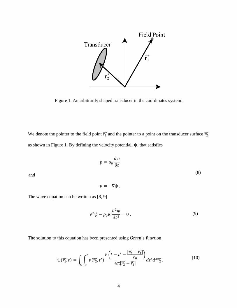
Figure 1. An arbitrarily shaped transducer in the coordinates system.

We denote the pointer to the field point 𝑟1 and the pointer to a point on the transducer surface 𝑟2 ,

as shown in Figure 1. By defining the velocity potential, ψ, that satisfies

𝑝 = ρ0

𝜕ψ

𝜕𝑡

and

𝑣 = −∇ψ .

(8)

The wave equation can be written as [8, 9]

∇2𝜓 − 𝜌0𝐾𝜕2𝜓

𝜕𝑡2= 0 . (9)

The solution to this equation has been presented using Green’s function

ψ(𝑟1 , 𝑡) = ∫ ∫ 𝑣(𝑟2 , 𝑡′)

δ (𝑡 − 𝑡′ −|𝑟2 − 𝑟1 |

𝑐0)

4π|𝑟2 − 𝑟1 |𝑑𝑡′𝑑2𝑟2

𝑡

0𝑆

. (10)

5

where 𝑣(𝑟2 , 𝑡) is the velocity at each point of transducer and each time instance. It is noteworthy

that Equation (10), in essence, is summing up the emitted waves from each point of the transducer

at the point of interest.

Assuming the velocity can be decomposed into a time dependent term and a spatial

component such that 𝑣(𝑟2 , 𝑡) = 𝑣𝑒(𝑡)𝑎(𝑟2 ), Equation (10) can be written as the convolution in the

time domain

Ψ(𝑟1 , 𝑡) = 𝑣(𝑟2 , 𝑡′) ∗ ℎ𝑎(𝑟1 , 𝑟2 , 𝑡) (11)

where ℎ𝑎(𝑟1 , 𝑡) is the spatial impulse response and

ℎ𝑎(𝑟1 , 𝑡) = ∫ 𝑎(𝑟2 )δ (𝑡 − 𝑡′ −

|𝑟2 − 𝑟1 |𝑐0

)

4𝜋|𝑟2 − 𝑟1 |𝑑2𝑟2

𝑆

. (12)

Unlike regular impulse response, spatial impulse response is a function of spatial location and

time. In simple words, it identifies how a velocity impulse from the transducer is felt at a certain

location 𝑟1 and how this response changes over time 𝑡.

As can be seen by performing the above integrations for all points on the transducer the

resulting field for any points could be obtained. However, this is a cumbersome operation and

needs large scale computational resources. The method in Field II divides the transducer into

several squares or rectangles and calculates the field due to each of those rectangular shapes, rather

than treat them as a point source. This allows it to severely reduce the number of needed elements

to characterize the field due to an arbitrarily shaped transducer without sacrificing precision.

6

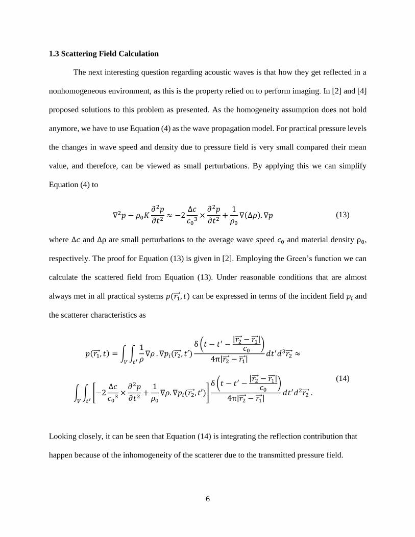
1.3 Scattering Field Calculation

The next interesting question regarding acoustic waves is that how they get reflected in a

nonhomogeneous environment, as this is the property relied on to perform imaging. In [2] and [4]

proposed solutions to this problem as presented. As the homogeneity assumption does not hold

anymore, we have to use Equation (4) as the wave propagation model. For practical pressure levels

the changes in wave speed and density due to pressure field is very small compared their mean

value, and therefore, can be viewed as small perturbations. By applying this we can simplify

Equation (4) to

∇2𝑝 − 𝜌0𝐾𝜕2𝑝

𝜕𝑡2≈ −2

Δ𝑐

𝑐03×

𝜕2𝑝

𝜕𝑡2+

1

𝜌0∇(∆𝜌). ∇𝑝 (13)

where Δ𝑐 and Δρ are small perturbations to the average wave speed 𝑐0 and material density ρ0,

respectively. The proof for Equation (13) is given in [2]. Employing the Green’s function we can

calculate the scattered field from Equation (13). Under reasonable conditions that are almost

always met in all practical systems 𝑝(𝑟1 , 𝑡) can be expressed in terms of the incident field 𝑝𝑖 and

the scatterer characteristics as

𝑝(𝑟1 , 𝑡) = ∫ ∫1

𝜌∇𝜌

𝑡′𝑉

. ∇𝑝𝑖(𝑟2 , 𝑡′)δ (𝑡 − 𝑡′ −

|𝑟2 − 𝑟1 |𝑐0

)

4π|𝑟2 − 𝑟1 |𝑑𝑡′𝑑3𝑟2 ≈

∫ ∫ [−2Δ𝑐

𝑐03×

𝜕2𝑝

𝜕𝑡2+

1

𝜌0∇𝜌. ∇𝑝𝑖(𝑟2 , 𝑡′)]

𝑡′𝑉

δ (𝑡 − 𝑡′ −|𝑟2 − 𝑟1 |

𝑐0)

4π|𝑟2 − 𝑟1 |𝑑𝑡′𝑑2𝑟2 .

(14)

Looking closely, it can be seen that Equation (14) is integrating the reflection contribution that

happen because of the inhomogeneity of the scatterer due to the transmitted pressure field.

7

CHAPTER 2

Overview of Ultrasonic Imaging Systems

This chapter gives an overview of various ultrasound imaging methodologies. Medical

application of ultrasound dates back to 1928 and, its modern usages, range from diagnosis to

therapy [10]. Therapeutic ultrasound became widespread in 1950 [11]. The diagnostic application

uses these waves to analyze living organs and cells and forms their image. Various types of

imaging are performed by transmitting a detection signal (usually a broadband pulse) and

collecting the reflected waves. Ultrasonic impedance mismatch (tissue boundaries) cause these

reflections and their corresponding location obtained based on the arrival times of received waves.

Ultrasound imaging has been favored for its non-invasive nature and relatively low-cost

implementation [12]. These imaging systems can be categorized based on their operation into

several groups. The remainder of this chapter discusses these methods and applications.

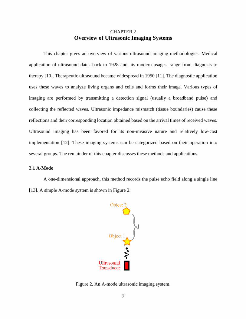
2.1 A-Mode

A one-dimensional approach, this method records the pulse echo field along a single line

[13]. A simple A-mode system is shown in Figure 2.

Figure 2. An A-mode ultrasonic imaging system.

8

The transmitted pulse creates two sets of reflections that are sensed by the receiver,

typically the transducer itself. Such a system has been simulated and the received waveform is

shown in Figure 3. Each cluster corresponds to one of the objects and are separated in time by the

distance between the two objects and the additional time for the transmitted pulse to get to the

second object and the echo field to be reflected from it. A-mode imaging has been used for sinusitis

diagnosis [14] and it has comparable performance for maxillary sinus infection diagnosis to

Computed Tomography (CT) [15]. Its compact implementation with a single transducer has made

it suitable for applications with size or weight limitations such as wearable devices [16, 17]. Also

it has been employed in ophthalmology.

Figure 3. Received echo pulse field for an A-mode system with two objects located 30 mm apart.

Excitation is a single 3 MHz sinusoidal pulse.

It can be readily seen that A-mode is sensitive to alignment between the objects it wants to

capture and its transducer.

9

2.2 B-Mode

This method, which is the most common ultrasound technique, forms a 2-D image [18]. Its

name is short for Brightness-Mode because the image is formed by depicting the intensity of

reflected wave envelope on a screen [19]. It can be viewed as an A-mode being repeated multiple

times to form the two-dimensional image. It has been implemented in many ways. A mechanical

approach to sweep across a region is reported in [20, 21, 22]. In this method a single transducer

was used with mechanical arms to tilt it to cover the Region of Interest (ROI). With introduction

of array transducers, arrays were used to eliminate the need for slow mechanical equipment,

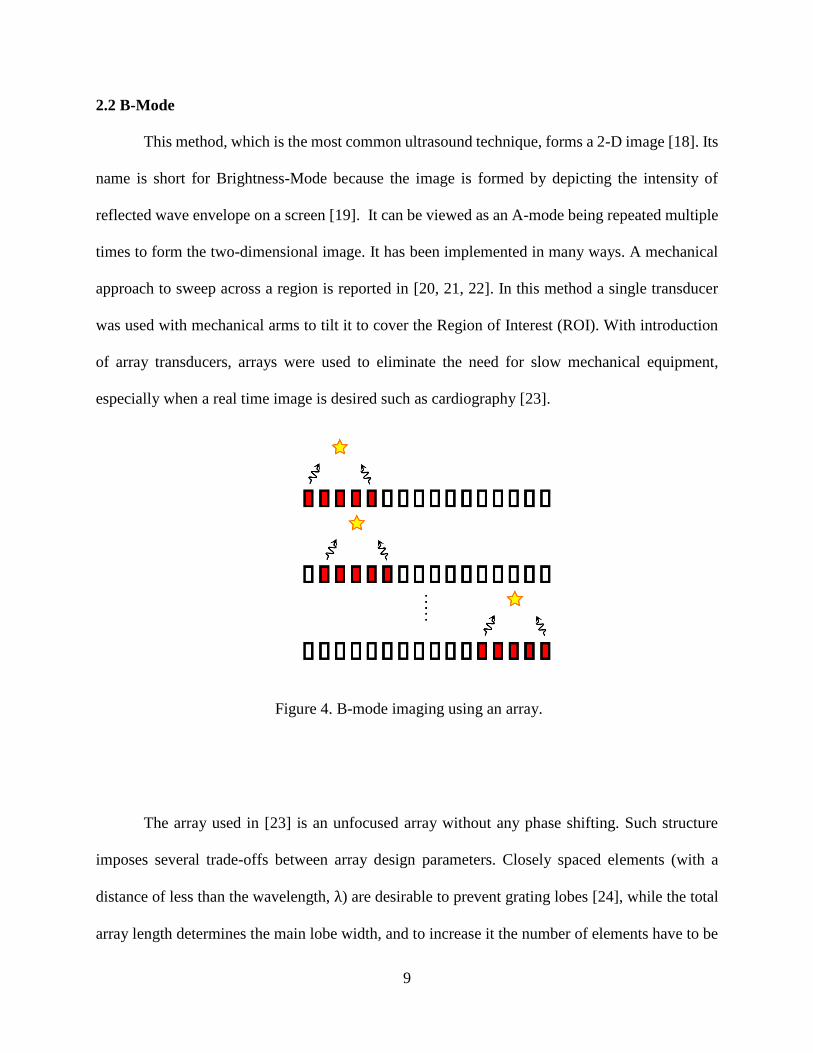
especially when a real time image is desired such as cardiography [23].

Figure 4. B-mode imaging using an array.

The array used in [23] is an unfocused array without any phase shifting. Such structure

imposes several trade-offs between array design parameters. Closely spaced elements (with a

distance of less than the wavelength, λ) are desirable to prevent grating lobes [24], while the total

array length determines the main lobe width, and to increase it the number of elements have to be

10

increased. An array used for B-mode imaging is shown in Figure 4. Usually several neighboring

cells are turned on simultaneously, as are shown by red cells in Figure 4, to have a wider effective

array and extend the near field region [1].

Phased arrays were able to decouple these trade-offs by forming a focused beam at a cost

of electrical complicity [23]. More intuition into a phased array operation can be obtained by

simple two element system is shown in Figure 5.

Figure 5. Simple two element phase array.

For simplicity we assume the point of interest to be exactly on top of one of the elements.

We can see, assuming the point distance is much bigger than elements spacing

𝑟1 = √(𝑟22 + 𝑑2) ≈ 𝑟2 (1 +

𝑑2

2𝑟22) = 𝑟2 +

𝑑2

2𝑟2 . (15)

This implies the travel time for the pulse transmitted from the first element is longer than that for

the second element by

11

Δ𝑡 =𝑟1 − 𝑟2

𝑐=

𝑑2

2𝑟2𝑐 (16)

where 𝑐 is the wave propagation speed. Therefore, by ensuring 𝑡1 = 𝑡2 + Δ𝑡 in Figure 5 then two

pulses will arrive simultaneously at the point of interest and will add constructively upon their

arrival at the particular point of focus. However, for other points, as their arrival times vary they

will not add on. This is the basic notion for beam forming with phased array. It is noteworthy that

the constructive addition of the amplitudes at the focus point lead to a higher value compared to

the other points (a narrower beam) as the number of elements increases. Although this discussion

was limited to the transmit case, the receiver follows the same principles due to reciprocity.

As it is readily seen, they need completely independent transmit and receive paths with

dedicated blocks to delay the signals, which is the reason for their sophistication and excessive

cost. With the ability to steer the beam, the width of the captured image is no longer determined

by array physical length [1] and the arrays can be made smaller. Also generating narrower beams

increases the image resolution [25].

2.3 C-Mode

Constant depth or C-mode imaging is essentially different compared to the two discussed

types of ultrasonic imaging systems. In this method instead of forming the image by reflection

from tissue boundaries, it is formed by the portion of transmission signal that passes through the

tissue.

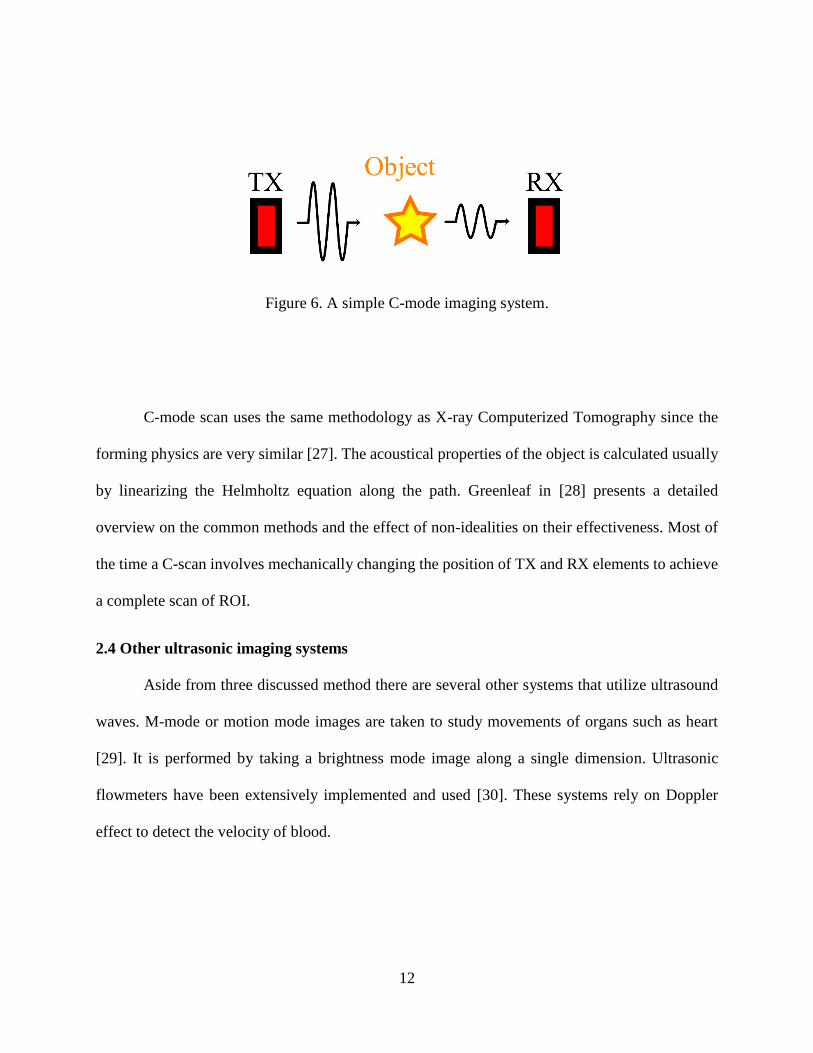
As Figure 6 depicts, in this method transmitter and receiver are placed on different sides of

the object that will be imaged and the portion of the wave that passes through it is recorded by RX.

In this method two main sets of information can be obtained. First, the total attenuation in the

signal path through the object. Second, ultrasound speed in the object [1, 26].

12

Figure 6. A simple C-mode imaging system.

C-mode scan uses the same methodology as X-ray Computerized Tomography since the

forming physics are very similar [27]. The acoustical properties of the object is calculated usually

by linearizing the Helmholtz equation along the path. Greenleaf in [28] presents a detailed

overview on the common methods and the effect of non-idealities on their effectiveness. Most of

the time a C-scan involves mechanically changing the position of TX and RX elements to achieve

a complete scan of ROI.

2.4 Other ultrasonic imaging systems

Aside from three discussed method there are several other systems that utilize ultrasound

waves. M-mode or motion mode images are taken to study movements of organs such as heart

[29]. It is performed by taking a brightness mode image along a single dimension. Ultrasonic

flowmeters have been extensively implemented and used [30]. These systems rely on Doppler

effect to detect the velocity of blood.

13

CHAPTER 3

Proposed Methodology

In this chapter our proposed method for ultrasonic imaging will be discussed.

3.1 Unfocused array

In the imaging methods discussed in CHAPTER 2 images were taken along a single

dimension (multiple one-dimension images were taken for B-mode). The underlying reason for

employing such methods is the way each point of the received wave is mapped to a physical

location in the object from which we are taking an image. This mapping is done using only the

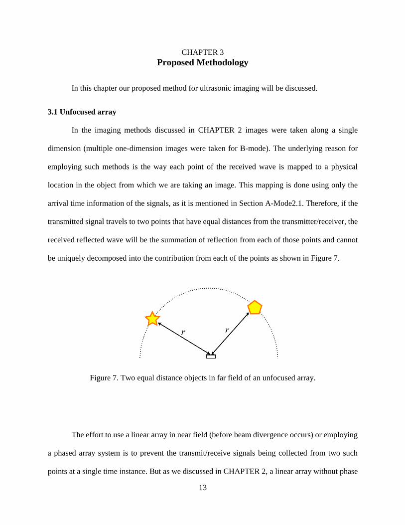
arrival time information of the signals, as it is mentioned in Section A-Mode2.1. Therefore, if the

transmitted signal travels to two points that have equal distances from the transmitter/receiver, the

received reflected wave will be the summation of reflection from each of those points and cannot

be uniquely decomposed into the contribution from each of the points as shown in Figure 7.

Figure 7. Two equal distance objects in far field of an unfocused array.

The effort to use a linear array in near field (before beam divergence occurs) or employing

a phased array system is to prevent the transmit/receive signals being collected from two such

points at a single time instance. But as we discussed in CHAPTER 2, a linear array without phase

14

shifting suffers from several severe trade-offs in its size, resolution, and array elements. A phased

array can overcome some of these drawbacks at a price of complexity and overall system cost. Our

proposed method will offer a solution to decouple these challenges.

3.2 Proposed method

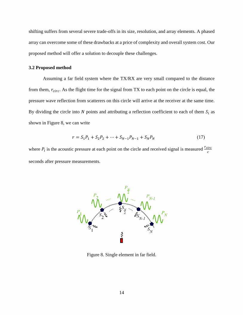
Assuming a far field system where the TX/RX are very small compared to the distance

from them, 𝑟𝑐𝑖𝑟𝑐. As the flight time for the signal from TX to each point on the circle is equal, the

pressure wave reflection from scatterers on this circle will arrive at the receiver at the same time.

By dividing the circle into 𝑁 points and attributing a reflection coefficient to each of them 𝑆𝑖 as

shown in Figure 8, we can write

𝑟 = 𝑆1𝑃1 + 𝑆2𝑃2 + ⋯+ 𝑆𝑁−1𝑃𝑁−1 + 𝑆𝑁𝑃𝑁 (17)

where 𝑃𝑖 is the acoustic pressure at each point on the circle and received signal is measured 𝑟𝑐𝑖𝑟𝑐

𝑐

seconds after pressure measurements.

Figure 8. Single element in far field.

15

The pressure field at each point can be easily calculated using the method discussed in Section 1.2

through Equations (10), (11), and (12). However, Equation (17) cannot be solved to find

𝑆1, 𝑆2, … , 𝑆𝑁, by transmitting a pulse in the configuration of Figure 8 and receiving the reflections,

because the number of equations is less than the number of unknowns. However, if this experiment

can be repeated multiple times and we can generate a new pressure pattern on the circle each time,

we will be able to find a solution to the system of equations

𝑟1 = 𝑆1𝑃1,1 + 𝑆2𝑃2,1 + ⋯+ 𝑆𝑁−1𝑃𝑁−1,1 + 𝑆𝑁𝑃𝑁,1

𝑟2 = 𝑆1𝑃1,2 + 𝑆2𝑃2,2 + ⋯+ 𝑆𝑁−1𝑃𝑁−1,2 + 𝑆𝑁𝑃𝑁,2

…

𝑟𝑀 = 𝑆1𝑃1,𝑀 + 𝑆2𝑃2,𝑀 + ⋯+ 𝑆𝑁−1𝑃𝑁−1,𝑀 + 𝑆𝑁𝑃𝑁,𝑀

(18)

where 𝑀 is the number of experiment repetitions. By having 𝑀 > 𝑁 , the system of equations in

Equation (18) is overdetermined and can be solved to find scattering coefficients 𝑆𝑖 for 1 ≤ 𝑖 ≤

𝑁.

3.2.1 Generating independent patterns on the circle

The possibility of employing methodology discussed earlier relies on our ability to generate

an arbitrary number of independent pressure profiles in the far field. It is obvious that a single

element is not capable of doing this task and using an array is inevitable.

In order to understand the required mechanism to generate various profiles on this circle,

we have to calculate a general expression for the pressure on a circular path from an array. Many

sources including [1, 24, 31] have solved this problem using similar approaches based on the

material developed in Section 1.2. We will use the same approach here.

16

Assume an array with 𝑁𝑎 elements that have a spacing of 𝑑. These elements are assumed

to be point sources and have very small width for simplicity. The overall array length is much

smaller than the circle radius (i.e. (𝑁𝑎 − 1)𝑑 ≪ 𝑟). More general cases can be found in [1, 24, 31].

Each element is having its own pressure field 𝑔𝑖(𝑡) = 𝑎𝑖𝑒𝑗𝜔𝑡. Here 𝑎𝑖 denote the amplitude of the

transmitted signal from each TX element. It must be noted this expression is not entirely correct

for our case, as we do not employ a continuous wave sinusoid but rather a short duration sinusoidal

pulse. However, the continuous wave expression eases the mathematical analysis significantly and

can be used to gain better understanding for the case where pulses are transmitted.

The described configuration is depicted in Figure 9. The reader should pay attention that

the scales in this figure are not realistic. The circle radius in far field operation must be much

bigger than the total array aperture.

Figure 9. Array pressure calculation on circle.

The acoustic pressure field contribution of the element 𝑖 of the array at our point of interest is

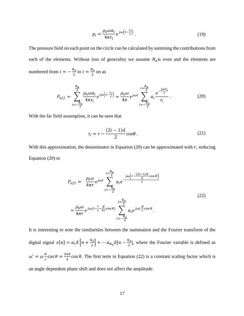
17

𝑝𝑖 =𝜌0𝜔𝑎𝑖

4𝜋𝑟𝑖𝑒𝑗𝜔(𝑡−

𝑟𝑖𝑐

) . (19)

The pressure field on each point on the circle can be calculated by summing the contributions from

each of the elements. Without loss of generality we assume 𝑁𝑎is even and the elements are

numbered from 𝑖 = −𝑁𝑎

2 to 𝑖 =

𝑁𝑎

2 on as

𝑃𝑒𝑓𝑓 = ∑𝜌0𝜔𝑎𝑖

4𝜋𝑟𝑖𝑒𝑗𝜔(𝑡−

𝑟𝑖𝑐

)

𝑁𝑎2

𝑖=−𝑁𝑎2

=𝜌0𝜔

4𝜋𝑒𝑗𝜔𝑡 ∑ 𝑎𝑖

𝑒−𝑗𝜔𝑟𝑖

𝑐

𝑟𝑖 .

𝑖=𝑁𝑎2

𝑖=−𝑁𝑎2

(20)

With the far field assumption, it can be seen that

𝑟𝑖 ≈ 𝑟 −(2𝑖 − 1)𝑑

2cosθ . (21)

With this approximation, the denominator in Equation (20) can be approximated with 𝑟, reducing

Equation (20) to

𝑃𝑒𝑓𝑓 = 𝜌0𝜔

4𝜋𝑟𝑒𝑗𝜔𝑡 ∑ 𝑎𝑖𝑒

−𝑗𝜔(𝑟−

(2𝑖−1)𝑑2

cos𝜃)

𝑐

𝑖=𝑁𝑎2

𝑖=−𝑁𝑎2

=𝜌0𝜔

4𝜋𝑟𝑒𝑗𝜔(𝑡−

𝑟𝑐−

𝑑2𝑐

cos𝜃) ∑ 𝑎𝑖𝑒𝑗𝜔𝑖

𝑑𝑐

cos𝜃 .

𝑖=𝑁𝑎2

𝑖=−𝑁𝑎2

(22)

It is interesting to note the similarities between the summation and the Fourier transform of the

digital signal 𝑥[𝑛] = 𝑎1𝛿 [𝑛 +𝑁𝑎

2] + ⋯𝑎𝑁𝑎

𝛿[𝑛 −𝑁𝑎

2], where the Fourier variable is defined as

𝜔′ = 𝜔𝑑

𝑐cos 𝜃 =

2𝜋𝑑

𝜆cos 𝜃. The first term in Equation (22) is a constant scaling factor which is

an angle dependent phase shift and does not affect the amplitude.

18

Equation (22) suggests different sets of 𝑎𝑖s in each experiment results in different pressure profile.

If the experiment has been done two times, one time with the amplitude sets of {𝑎𝑖 , −𝑁𝑎

2≤ 𝑖 ≤

𝑁𝑎

2}

and the second time with {𝑎𝑖′, −

𝑁𝑎

2≤ 𝑖 ≤

𝑁𝑎

2}. The resulting pressure profiles (𝑃𝑒𝑓𝑓, 𝑃𝑒𝑓𝑓′) will not

be linearly independent if for all 𝜃 values the pressures are linearly related. This will happen if and

only if the vectors (𝑎−

𝑁𝑎2

, … , 𝑎𝑁𝑎2

) and (𝑎′−

𝑁𝑎2

, … , 𝑎′𝑁𝑎2

) are linearly dependent. Therefore, by using

random numbers as amplitudes for each experiment we will be able to obtain linearly independent

equations with high probability.

By forming the various equations of Equation (18) in matrix form we see that

(

𝑟1𝑟2⋮

𝑟𝑀

) = (

𝑃1,1 ⋯ 𝑃𝑁,1

⋮ ⋱ ⋮𝑃𝑀,1 ⋯ 𝑃𝑀,𝑁

)(

𝑆1

𝑆2

⋮𝑆𝑀

) (23)

which has dimensions

𝑟𝑀×1 = 𝑃𝑀×𝑁 × 𝑆𝑀×1 (24)

The rank of the pressure matrix 𝑃𝑀×𝑁 is a measure of independence of these equations. However,

because 𝑎𝑖s are always a real number, 𝑃𝑒𝑓𝑓, which is their Fourier transform, will always be an

even function of cos 𝜃 and symmetric around 𝜃 =𝜋

2. This is problematic since we will not be able

to differentiate form the scatterers located at 𝜃′ and 𝜋 − 𝜃′ . This implies that we have to

incorporate imaginary coefficients to mitigate this matter. But it should be noted that the imaginary

parts, which are implemented as phase shifts or delays, do not need to be as sophisticated as the

ones used in a phased array. We will discuss this more in Section 3.3.

19

Another point that needs to be paid attention to is that 𝑎𝑖s must have a zero mean. The

reason is that: if we denote the 𝑎𝑖average by 𝜇𝑎the Equation (22) can be rearranged into

𝑃𝑒𝑓𝑓 = 𝜌0𝜔

4𝜋𝑟𝑒𝑗𝜔(𝑡−

𝑟𝑐−

𝑑2𝑐

cos𝜃)

[

∑ (𝑎𝑖 − 𝜇𝑎)𝑒𝑗𝜔𝑖 𝑑𝑐

cos𝜃

𝑖=𝑁𝑎2

𝑖=−𝑁𝑎2

+ ∑ 𝜇𝑎𝑒𝑗𝜔𝑖 𝑑𝑐

cos𝜃

𝑖=𝑁𝑎2

𝑖=−𝑁𝑎2 ]

=𝜌0𝜔

4𝜋𝑟𝑒𝑗𝜔(𝑡−

𝑟𝑐−

𝑑2𝑐

cos𝜃) ∑ (𝑎𝑖 − 𝜇𝑎)𝑒𝑗𝜔𝑖 𝑑𝑐

cos𝜃

𝑖=𝑁𝑎2

𝑖=−𝑁𝑎2

+𝜌0𝜔𝜇𝑎

4𝜋𝑟𝑒𝑗𝜔(𝑡−

𝑟𝑐−

𝑑2𝑐

cos𝜃) ∑ 𝑒𝑗𝜔𝑖 𝑑𝑐

cos𝜃

𝑖=𝑁𝑎2

𝑖=−𝑁𝑎2

.

(25)

Figure 10. Pressure of an array with 100 elements and spacing of 𝜆

15. (a): Non-zero average

pressures (b): Zero average pressure.

The second part of Equation (25) is the Fourier transform of a pulse which will be a Sinc function,

or in limits of a wide pulse close to an impulse. This creates a deterministic part with a big peak in

20

the pressure pattern. Although the 𝑃𝑀×𝑁 matrix still will be full rank, and mathematically, the

system of equations in Equation (23) could be solved, the design of the following receiver will be

challenging. Figure 10 shows two cases of pressure profiles. The phase of each TX element is

randomly selected between 0 and 𝜋

2 in each experiment to create asymmetry.

3.2.2 Solving Matrix equation

The system of equations shown in Equation (23) might be overdetermined if we choose

𝑀 > 𝑁. The Least Squared (LS) method is the most well-developed form of solution for such

problems. The problem statement is as follows. For equation 𝐴𝑀×𝑁𝑥𝑁×1 = 𝑏𝑀×1, the LS solution

is found such that ‖𝐴𝑀×𝑁𝑥𝑁×1 − 𝑏𝑀×1‖2 is minimized, where the operator ‖ . ‖2denotes the 𝑀

dimensional squared distance from the 𝑀 dimensional origin.

The solution to the LS problem is 𝑥𝑁×1∗ = ((𝐴𝑀×𝑁)𝑇𝐴𝑀×𝑁)−1 𝑏𝑀×1. However, this solution might

have no physical meaning in our case where the scattering factor is a positive number. The

optimization problem might offer a solution that has negative values and offers a lower squared

error, but does not correspond to any physical scenario. As a result, we have to solve a constrained

problem where the variables are subject to 𝑥 ≥ 0. We employed the active-set method [32, 33].

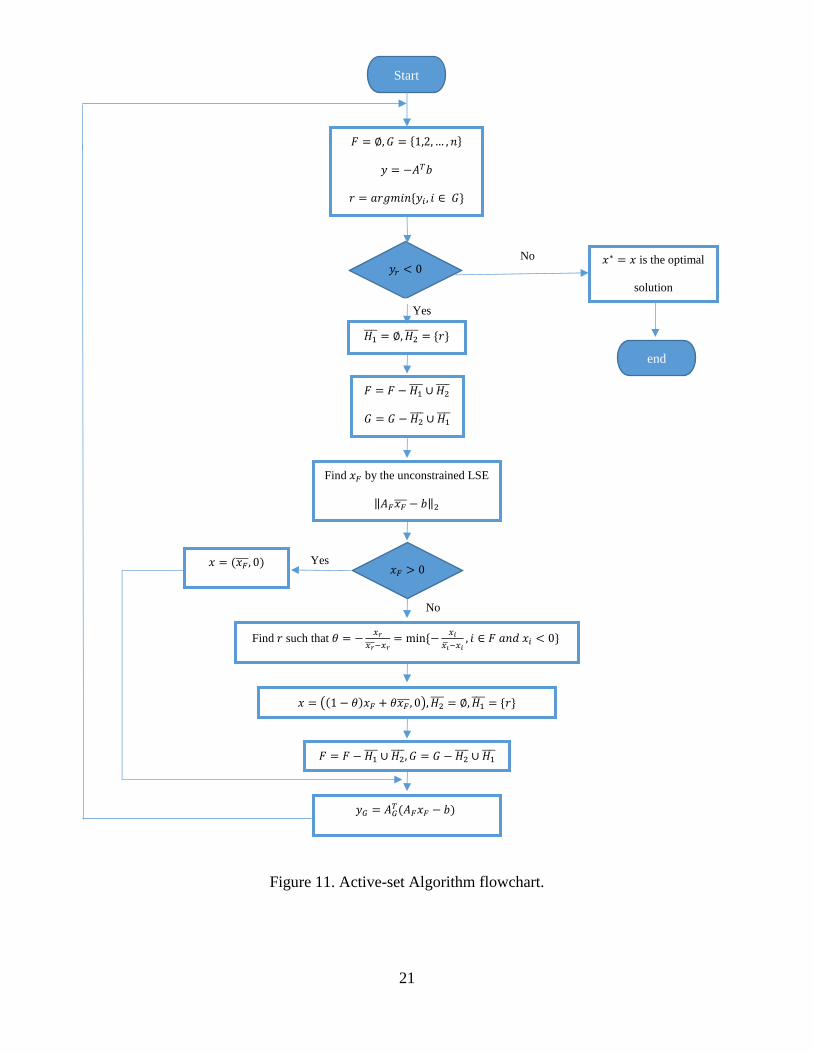
The flow chart of this algorithm is shown in Figure 11. In the flow chart the following notation

has been used: 𝐹 and 𝐺 are two sets such that 𝐹 ∪ 𝐺 = {1,2, … , 𝑛} and 𝐹 ∩ 𝐺 = ∅. The columns

of matrix 𝐴 is also divided into 𝐴 = [𝐴𝐹 , 𝐴𝐺] where |𝐹| and |𝐺| determine 𝐴𝐹 and 𝐴𝐺 sizes. 𝑥 and

𝑦 are also divided similarly to 𝑥 = (𝑥𝐹, 𝑥𝐺) and 𝑦 = (𝑦𝐹, 𝑦𝐺).

21

Figure 11. Active-set Algorithm flowchart.

𝐹 = ∅, 𝐺 = {1,2,… , 𝑛}

𝑦 = −𝐴𝑇𝑏

𝑟 = 𝑎𝑟𝑔𝑚𝑖𝑛{𝑦𝑖 , 𝑖 ∈ 𝐺}

𝑦𝑟 < 0

Start

𝑥∗ = 𝑥 is the optimal

solution

No

Yes

𝐻1 = ∅, 𝐻2

= {𝑟}

𝐹 = 𝐹 − 𝐻1 ∪ 𝐻2

𝐺 = 𝐺 − 𝐻2 ∪ 𝐻1

Find 𝑥𝐹 by the unconstrained LSE

‖𝐴𝐹𝑥𝐹 − 𝑏‖2

Yes 𝑥 = (𝑥𝐹 , 0)

𝑥𝐹 > 0

Find 𝑟 such that 𝜃 = −𝑥𝑟

𝑥𝑟 −𝑥𝑟= min {−

𝑥𝑖

𝑥��−𝑥𝑖, 𝑖 ∈ 𝐹 𝑎𝑛𝑑 𝑥𝑖 < 0}

No

end

𝑥 = ((1 − 𝜃)𝑥𝐹 + 𝜃𝑥𝐹 , 0),𝐻2 = ∅, 𝐻1

= {𝑟}

𝐹 = 𝐹 − 𝐻1 ∪ 𝐻2

, 𝐺 = 𝐺 − 𝐻2 ∪ 𝐻1

𝑦𝐺 = 𝐴𝐺𝑇(𝐴𝐹𝑥𝐹 − 𝑏)

22

3.3 Practical implementation

The system of equations in Equation (23) incorporates each experiment into a single

equation. However, the waveform received and transmitted as well as the pressure on each point

on the circle are short duration sinusoidal pulses in each experiment. In order to do so, we have to

associate a single number to each short duration pulse. Two possible candidates are the peak

magnitude and the square root of the power (to maintain a magnitude notion in the measure). The

latter was selected in this approach to provide a better estimation of the scatterer. This means that

in Equation (23) each 𝑃𝑖,𝑗 and 𝑟𝑖 are represented by the corresponding sinusoidal pulses square root

power.

3.3.1 2D Image Formation

The discussion so far has been focused on a single dimension image along a circular path. In

this section we will discuss how we obtain a complete 2D image by our method.

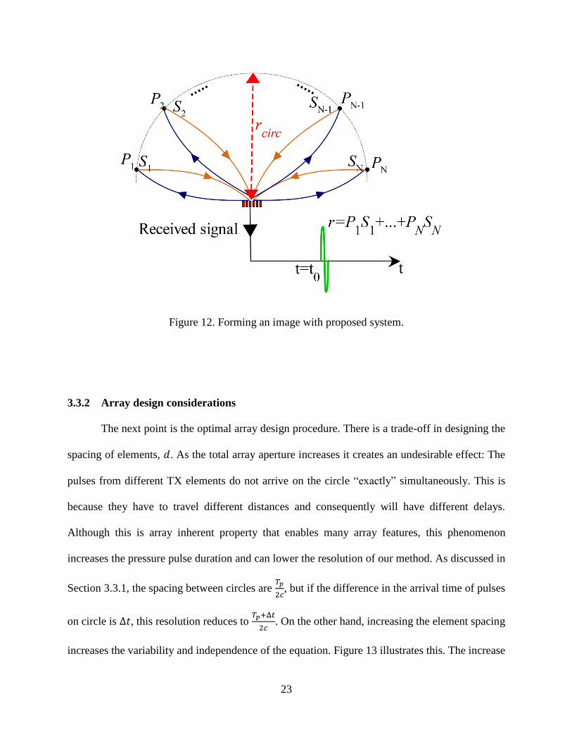
The reflections from scatterers lying on a circular path arrive simultaneously at the receiver

as shown in Figure 12. In this figure the received time of the pulse, 𝑡0, equals 𝑟𝑐𝑖𝑟𝑐

2𝑐. To form a 2D

image, the total received signal is divided into segments that correspond to a circular path with a

certain radius which is determined by the received time of that segment. Each segment length and

subsequently the spacing between circular paths is determined by the pulse duration, 𝑇𝑝. Following

this method the 𝑛𝑡ℎ segment will correspond to the circle with 𝑟𝑐𝑖𝑟𝑐 =(𝑛−1)𝑇𝑝

2𝑐 and 𝑐 is the acoustic

wave speed. The image of each of these circular paths are calculated to form the complete two

dimensional image.

23

Figure 12. Forming an image with proposed system.

3.3.2 Array design considerations

The next point is the optimal array design procedure. There is a trade-off in designing the

spacing of elements, 𝑑. As the total array aperture increases it creates an undesirable effect: The

pulses from different TX elements do not arrive on the circle “exactly” simultaneously. This is

because they have to travel different distances and consequently will have different delays.

Although this is array inherent property that enables many array features, this phenomenon

increases the pressure pulse duration and can lower the resolution of our method. As discussed in

Section 3.3.1, the spacing between circles are 𝑇𝑝

2𝑐, but if the difference in the arrival time of pulses

on circle is Δ𝑡, this resolution reduces to 𝑇𝑝+Δ𝑡

2𝑐. On the other hand, increasing the element spacing

increases the variability and independence of the equation. Figure 13 illustrates this. The increase

24

in the pressure matrix, 𝑃𝑀×𝑁, is plotted versus the equations number to unknown numbers ratio

(𝑀

𝑁) for three element spacings. In addition, the bigger the transmitter is, the further we need to be

to operate in the far field regime. The chosen spacing and element number are 𝜆/15 and 128,

respectively. It must be noted that the active-set algorithm requires a full rank matrix or it will not

converge.

Figure 13. Pressure variability with spacing, N=100, and M varied from 100 to 500.

3.4 Proposed system block diagram

To achieve a full rank matrix, Section 3.2.1 points out that, first, a zero-average amplitude

must be incorporated, and second, a phase shift is needed. The proposed method here will

implement both criteria.

25

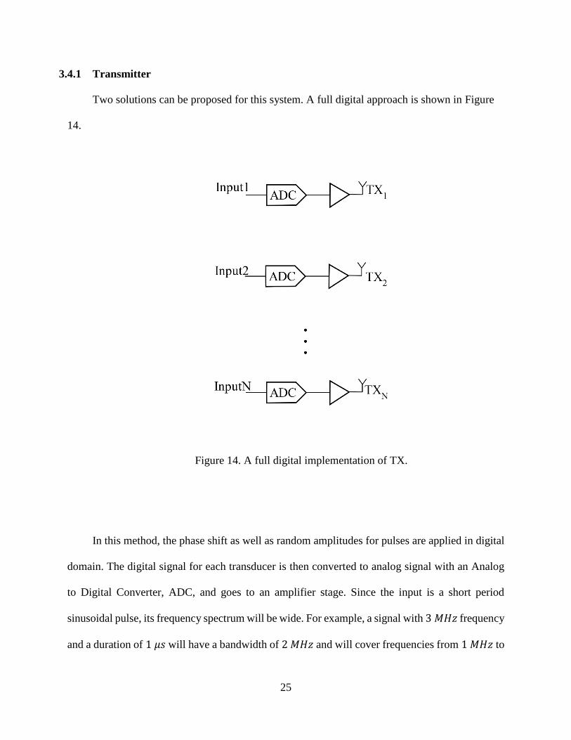
3.4.1 Transmitter

Two solutions can be proposed for this system. A full digital approach is shown in Figure

14.

Figure 14. A full digital implementation of TX.

In this method, the phase shift as well as random amplitudes for pulses are applied in digital

domain. The digital signal for each transducer is then converted to analog signal with an Analog

to Digital Converter, ADC, and goes to an amplifier stage. Since the input is a short period

sinusoidal pulse, its frequency spectrum will be wide. For example, a signal with 3 𝑀𝐻𝑧 frequency

and a duration of 1 𝜇𝑠 will have a bandwidth of 2 𝑀𝐻𝑧 and will cover frequencies from 1 𝑀𝐻𝑧 to

26

5 𝑀𝐻𝑧. With a 1 MHz guard band, the ADC sampling frequency will need to be higher than

12 𝑀𝐻𝑧. Even with a relatively relaxed requirements for other specifications, such a module will

be expensive. As a result of the fact that we need many ADCs for this configuration (as many as

array elements; e.g. 128), the overall system cost will be high.

An alternative approach is an analog implementation. Shown in Figure 15, this configuration

applies the phase shifting and random amplitude modulation in analog domain. The input which

is an analog pulse is fed into the transmitter chain for each transducer. This transmitter chain

consists of mux that randomly selects between 4 phases shifter outputs and a Programmable Gain

Amplifier, PGA. The gain coefficients 𝑎1, 𝑎2, … , 𝑎𝑁 will be a series of positive random numbers

that control the gain of the VGAs. Four different values of 𝜙 = {0, 90°, 180°, 270°} are possible

for the phase with equal probabilities. Because the gain and phase coefficients are independent,

the effective coefficient 𝑎𝑒𝑗𝜙has a zero mean.

𝐸(𝑎𝑒𝑗𝜙) = 𝐸(𝑎)𝐸(𝑒𝑗𝜙) = 𝐸(𝑎) (1

4𝑒0 +

1

4𝑒

𝑗𝜋2 +

1

4𝑒−𝑗𝜋 +

1

4𝑒

𝑗3𝜋2 ) = 0 . (26)

It must be noted that the complexity level of TX in this method is much less than a focused

array. First, it does not need as many phase shifters as a focused array. Second, the phase shifts

are not variable and can take only four distinct values.

27

Figure 15 An analog implementation of TX.

Such phase shifters can be easily made by a transmission line, which at conventional biomedical

ultrasonic frequencies, will be tens of micrometer long.

28

3.4.2 Receiver architecture

The receiver in the proposed system does not require phase shifters or amplitude

modulations. This is mainly because our system wants to collect reflected pulses from the entire

space to be able to associate scattering values to each circular path. The received signal used in

this method is the summation of received signal from each RX element.

29

CHAPTER 4

Experimental Results

In this chapter the result of the proposed methodology is presented. The simulations have

been done using FIELD II platform1. This software provides a tool for rapid ultrasonic simulation.

Its basis of operation has been discussed in detail in [5]. The used array is has 128 elements with

spacing of 𝜆

15= 34.2 𝜇𝑚. The element width is

𝜆

150= 3.4 𝜇𝑚.

4.1 Scattering value result along a circular path

As it was described in Section 3.2, our proposed method is capable of finding scattering

values on a circle. To verify that a high density scatterer is placed at 𝑥 = −20 𝑚𝑚 and 𝑧 =

113.2 𝑚𝑚, which is located at a circle with 𝑟𝑐𝑖𝑟𝑐 = √𝑥2 + 𝑧2 ≈ 115 𝑚𝑚. The brightness mode

result of scattering value along this circle is shown below.

Figure 16 One dimensional image of a single scatterer at 𝑥 = −20 𝑚𝑚 on a circular path with

𝑟𝑐𝑖𝑟𝑐 = 115 𝑚𝑚.

The bright line at 𝑥 = −20 𝑚𝑚 shows that the scatterer location is detected correctly.

The next level verification of the methodology is to assess its performance with multiple

scatterer clusters. We placed two clusters of high density scatterers on the circle of 115𝑚𝑚 radius.

1 Available online at http://field-ii.dk//.

30

We add one cluster at 𝑥 = 10 𝑚𝑚 and 𝑧 = 114.5 𝑚𝑚 and the captured image is depicted in Figure

17. Two lines at 𝑥 = −20 𝑚𝑚 and 𝑥 = 10 𝑚𝑚 show both scatterers have been captured

accurately.

Figure 17. One dimensional image of two scatterers at 𝑥 = −20 𝑚𝑚 and 𝑥 = 10 𝑚𝑚 on a

circular path with 𝑟𝑐𝑖𝑟𝑐 = 115 𝑚𝑚.

4.2 Full 2D image

By using the aforementioned method, we take a 2D image of two circular shaped cysts with

a radius of 5 mm.

31

It should be noted that to get the 2D image, scattering values along circles must be unwrapped to

map into cartesian coordinates. We can see that the shapes of cysts and their radiuses are captured.

4.3 Performance in presence of imperfections

Figure 19. Noise sensitivity of scatterer detection (a) SNR=20 dB (b) SNR=0 dB

Figure 18. 2D image. Left the original scatterers location, right captured image.

32

The method used in this work might seem vulnerable to noise or absolute values of transducer

amplitudes and phases, therefore, its sensitivity was simulated. To measure noise tolerance, we

added random white noise to the received signal. This can model the thermal noise of the electronic

interfaces accurately. However, the noise sources in the real living cell could be more complicated.

Nonetheless, this experiment can give us an idea of the robustness of our method to noise. The

simulations show that by varying the noise power even to the same level as the received signal, no

major degradation in image accuracy.

Figure 19 shows two results with SNR of 0 dB and 20 dB. The two bright lines are visible at

𝑥 = −20 𝑚𝑚 and 𝑥 = 10 𝑚𝑚 in both cases yet some error is also present which manifests itself

as detection of small scatterers at a few locations (visible in Figure 19 as faded lines).

Besides random noise, we need to investigate our system performance in presence of other

error sources. One of these non-idealities that seem to have a great consequence in our approach

is the absolute gain and phase error in each path. This is crucial because our calculation of the

pressure field at each point relies on the assumption that the TX chains transmitted signals are

exactly known, which might not be true if these paths experience gain and phase error. Our

proposed system performance in presence of these imperfections is examined by additionally

introducing them into our model. This is modeled by associating random gain and phase errors to

each TX chain. The errors are modeled by a gaussian distribution that has an rms of 20% of the

average gain. This artifact causes an additional low brightness line on the far right of the image.

33

Figure 20. Sensitivity of scatterer detection to 20% rms gain and phase error

4.4 Implementation with binary coefficients

As it was discussed in CHAPTER 3, the coefficients of the TX transducers need to be zero-

average, and random. There is no criteria on the numerical values they can take. This shows the

potential to use binary values for the magnitude (i.e. |𝑎𝑖| = 0 or 1), which greatly simplifies the

design of the 𝑉𝐺𝐴s in Figure 15. This implementation was used to take the picture of the two

scatterer clusters at 𝑥 = −20 𝑚𝑚 and 𝑥 = 10 𝑚𝑚.

Figure 21. Image of two scatterers at 𝑥 = −20 𝑚𝑚 and 𝑥 = 10 𝑚𝑚 on a circular path with

𝑟𝑐𝑖𝑟𝑐 = 115 𝑚𝑚 with binary TX coefficients.

It can be seen that the location of both scatterers are predicted correctly.

34

CHAPTER 5

Summary and Conclusions

In this work we presented a method for ultrasonic imaging using random signals. The

proposed approach employs randomly scaled short duration sinusoidal pulses and unlike currently

used methods, does not rely on generating narrow beams.

The proposed method is fully capable of capturing the essence of a biomedical cyst. While

only a proof of concept has been done in this research, there are several potential benefits. Relative

to conventional imaging systems, it can be implemented in a very small size and a low cost. Its

noise performance was examined and showed robust behavior. Although it is needed to perform

an active set algorithm to compute the image, the pressure matrix can be calculated ahead of time

and stored in the digital signal processor. The computation cost and time is moderate and must be

noted that this overhead enables us to capture the full image of the entire space after the repetitions.

This is comparable to a conventional device with a phased array having to focus to different points

and perform imaging multiple times.

The proposed method will need a calibration for the magnitude of transmitter chains, similar

to a conventional phased array system, but it does not require any phase calibration as the phase

relationships are fixed and are originated from shared phase shifters.

5.1 Future work

Although the concept of the method and some of its main challenges have been solved in

this research, it still needs to be further developed for full practical application.

The method needs to be used for taking an image of a living tissue to fully show its capability,

and, also, the challenges that it might face. This would require enhancing the dynamic range of the

35

method, because a large scatterer along a circular path could block a much smaller one on the same

path, as the reflected wave would be mostly dominated by the large one. Also a more realistic

noise model could be used to reassess the noise sensitivity.

The final step in fully validating the methodology requires physical implementation. An

array with suitable sizing must be selected, preferably from of-the-shelf products and excited using

our described method. The processing can still take place on a Personal Computer (PC) in the

prototype, but could be moved to a microprocessor for mass production.

36

Bibliography

[1] D. A. Christensen, Ultrasonic Bioinstrumentation, New York: Wiley, 1988.

[2] J. A. Jensen, "A model for the propagation and scattering of ultrasound in tissue," The

Journal of the Acoustical Society of America, vol. 89, no. 1, pp. 189-191, 1991.

[3] D. J. Griffiths, Introduction to Electrodynamics, Upper Saddle River, N.J.: Prentice Hall,

1999.

[4] G. C. Gore and S. Leeman, "Ultrasonic backscattering from human tissue: a realistic

model," Physics in Medicine & Biology, vol. 22, no. 2, p. 317, 1977.

[5] J. A. Jensen and N. B. Svendsen, "Calculation of Pressure Fields from Arbitrarily Shaped,

Apodized, and Excited Ultrasound Transducers," IEEE Transaction ON Ultrasonics.

Ferroelectrics And Frequency Control, vol. 39, pp. 262-267, 1992.

[6] G. R. Harris, "Review of transient field theory for a baffled planar piston," The Journal of

the Acoustical Society of America, vol. 70, pp. 10-20, 1981.

[7] G. R. Harris, "Transient field of a baffled planar piston having an arbitrary vibration

amplitude distribution," The Journal of the Acoustical Society of America, vol. 70, pp. 186-

204, 1981.

[8] P. R. Stepanishen, "The Time‐Dependent Force and Radiation Impedance on a Piston in a

Rigid Infinite Planar Baffle," The Journal of the Acoustical Society of America, vol. 49, no.

3B, p. 841, 1971.

37

[9] G. E. Tupholme, "Generation of acoustic pulses by baffled plane pistons," Mathematika,

vol. 16, no. 2, pp. 209-224, 1969.

[10] J. F. Herrick and F. H. Krusen, "Ultrasound and Medicine (A Survey of Experimental

Studies)," The Journal of the Acoustical Society of America , vol. 26, no. 2, pp. 236-240,

1954.

[11] D. L. Miller, N. B. Smith, M. R. Bailey, G. J. Czarnota, K. Hynynen and I. Makin,

"Overview of Therapeutic Ultrasound Applications and Safety Considerations," Journal of

Ultrasound in Medicine, vol. 31, no. 4, pp. 623-634, 2012.

[12] M. G. S. J. Sutton and J. D. Rutherford, Clinical Cardiovascular Imaging, Amesterdam,

The Netherlands: Elsevier, 2004.

[13] A. S. F. &. J. D. Carovac, "Application of ultrasound in medicine," Acta Informatica

Medica : AIM : Journal of the Society for Medical Informatics of Bosnia & Herzegovina,

vol. 19, no. 3, pp. 168-171, 2011.

[14] H. Varonen, M. Makela, S. Savolainen, E. Laara and J. Hilden, "Comparison of ultrasound,

radiography, and clinical examination in the diagnosis of acute maxillary sinusitis: A

systematic review," Journal of Clinical Epidemiology, vol. 53, no. 9, pp. 940-948, 2000.

[15] F. Lucchin, N. Minicuci, M. Ravasi, L. Cordella, M. Palù, M. Cetoli and P. Borin,

"Comparison of A-mode ultrasound and computed tomography: detection of secretion in

maxillary and frontal sinuses in ventilated patients," Intensive Care Medicine, vol. 22, no.

11, pp. 1265-1268, 1996.

38

[16] J.-Y. Guo, Y.-P. Zheng, Q.-H. Huang and X. Chen, "Dynamic monitoring of forearm

muscles using one-dimensional sonomyography system," Journal of Rehabilitation

Research & Development, vol. 45, no. 1, pp. 187-196, 2008.

[17] S. Sikdar, H. Rangwala, E. B. Eastlake, I. A. Hunt, A. J. Nelson, J. Devanathan, A. Shin

and J. J. Pancrazio, "Novel Method for Predicting Dexterous Individual Finger Movements

by Imaging Muscle Activity Using a Wearable Ultrasonic System," IEEE Transactions on

Neural Systems and Rehabilitation Engineering, vol. 22, no. 1, pp. 69-76, 2014.

[18] V. Chan and A. Perlas, "Basics of Ultrasound Imaging," in Atlas of Ultrasound-Guided

Procedures in Interventional Pain Management, New York, N. Y., Springer, 2011, pp. 13-

19.

[19] F. E. Barber, D. W. Baker, A. W. C. Nation, D. E. Strandness and J. M. Reid, "Ultrasonic

Duplex Echo-Doppler Scanner," IEEE Transactions on Biomedical Engineering, vol. 21,

no. 2, pp. 109-113, 1974.

[20] R. C. Eggleton and K. W. Johnston, "Real Time B-Mode Mechanical Scanning System,"

Proceedings of SPIE, vol. 47, pp. 96-100, 1957.

[21] R. C. Eggleton, "Ultrasound Visualization of the Dynamic Geometry of the Heart," in 2nd

World Congress on Ultrasound in Medicine, Rotterdam, 1973.

[22] F. L. Thurstone, "Electronic Beam Scanning for Ultrasonic Imaging," in 2nd World

Congress on Ultrasound in Medicine, Rotterdam, 1973.

39

[23] N. Bom, C. T. Lancee, G. V. Zwieten, F. E. Kloster and J. Roelandt, "Multiscan

Echocardiography I. Technical Description," Circulatiom, vol. 48, no. 5, pp. 1066-1074,

1973.

[24] A. Macovski, "Ultrasonic Imaging Using Arrays," Proceedings of the IEEE, vol. 67, no. 4,

pp. 484-495, 1979.

[25] O. Von Ramm and F. Thurstone, "Improved Resolution in Ultrasound Tomography," in

25th Annual Conference on Engineering in Medicine and Biology, 1972.

[26] J. F. Greenleaf and R. C. Bahn, "Signal Processing Methods for Transmission Ultrasonic

Computerized Tomography," in 1980 Ultrasonics Symposium, 1966.

[27] R. K. Mueller, M. Kaveh and G. Wade, "Reconstructive tomography and applications to

ultrasonics," Proceedings of IEEE, vol. 67, no. 4, pp. 567-587, 1979.

[28] J. F. Greenleaf, "Computerized tomography with ultrasound," Proceedings of IEEE, vol.

71, no. 3, pp. 330-337, 1983.

[29] M. Halliwell, "A tutorial on ultrasonic physics and imaging techniques," Proceedings of

Institution of Mechanical Engineers. Part H, Journal of Engineering in Medicine , vol.

224, no. 2, pp. 127-142, 2010.

[30] J. A. Jenses, "Algorithms for estimating blood velocities using ultrasound," Ultrasonics,

vol. 38, pp. 358-62, 2000.

40

[31] J. A. Jensen, Estimation of Blood Velocities Using Ultrasound: A Signal Processing

Approach, New York, N.Y.: Cambridge University Press, 1996.

[32] L. F. Portugal, J. J. Joaquim, J. Judice, L. N. Vicente, "A Comparison of Block Pivoting

and Interior Point Algorithms for Linear Least Squares Problems with Nonnegative

Values," Mathematics of Computation, vol. 63, pp. 625-643, 1994.

[33] Å. Björck, "A direct method for sparse least squares problems with lower and upper

bounds," Numerische Mathematik, vol. 54, no. 1, pp. 19-32, 1988.