BiologicalJournal ofthe Linnean Socieo (1999), 67: 529-584. With 12 figures Article ID: bij1.1999.0318, available online at http://www.idealibrary.com. on 10 E )r.L @ A null model for species richness gradients: bounded range overlap of butterflies and other rainforest endemics in Madagascar DAVID C. LEES* Biogeography and Conservation Luborato9 (Department of Entomology), The Natural Histo9 Museum, Cromwell Road, South Kensington, London SW7 5BD CLAIRE KREMEN Center for Conservation Biology, Dept. of Biological Sciences, Herrin Hall, Stanford Uniuersig, Stanford, Calgornia 943 05, U. S.A. LANTO ANDRIAMAMPIANINA Wldltji Conservation Socieg, B.P 8500, Ella Lova lanisoa, Soavimbahoaka, Antananarivo 101, Madagascar Received 1 December 1997; accepted for publication 10 January I999 Species richness has classically been thought to increase from the poles towards the Equator, and from high elevations down to sea-level. However, the largest radiation of butterflies in Madagascar, the subtribe Mycalesina (c. 67 spp.) does not exhibit such a monotonic pattern, either for empirical records or for interpolated species ranges. Instead, summation of mycalesine ranges generates a domed curve of species richness values approximately symmetric around mid latitudes within the island, a pattern most smoothly exhibited by the wider ranging and better known species, and a less symmetric curve peaking near mid elevations. Hotspots for the summation of 1 183 species ranges and seven out of the ten groups of insects and vertebrates analysed (butterflies, cicindelid and enariine melonthid beetles, ctenuchiine moths, chameleons, frogs, birds, lemurs, tenrecs, and rodents) also occur at both mid latitudes and elevations. The most strongly parabolic pattern is shown by animals (637 spp.) whose ranges are confined to the highly linear rainforest biome. This rainforest species richness curve is resilient in shape even after controlling for particular effects of area and irregular sample effort. In sharp contrast, at least eight different environmental parameters for the rainforest biome tend to increase monotonically towards the northern, more tropical, boundary, a trend evident only in species richness gradients of more narrow-ranging species. The one-dimensional latitudinal species richness curves and hotspots observed in fact best reflect overall the geometric predictions of a null model for ranked range size partitions of * Corresponding author. Present address: Department of Palaeontology, The Natural History Museum, Cromwell Road, South Kensington, London SW7 5BD. e-mail: dcl @nhm.ac.uk 0024-4066/99/080529+56 $30.00 0 1999 The Linnean Society of London 529
Transcript
BiologicalJournal ofthe Linnean Socieo (1999), 67: 529-584. With 12 figures
Article ID: bij1.1999.0318, available online at http://www.idealibrary.com. on 10 E )r.L @
A null model for species richness gradients: bounded range overlap of butterflies and other rainforest endemics in Madagascar
DAVID C. LEES*
Biogeography and Conservation Luborato9 (Department o f Entomology), The Natural Histo9 Museum, Cromwell Road, South Kensington, London SW7 5BD
CLAIRE KREMEN
Center for Conservation Biology, Dept. o f Biological Sciences, Herrin Hall, Stanford Uniuersig, Stanford, Calgornia 943 05, U. S.A.
Received 1 December 1997; accepted fo r publication 10 January I999
Species richness has classically been thought to increase from the poles towards the Equator, and from high elevations down to sea-level. However, the largest radiation of butterflies in Madagascar, the subtribe Mycalesina (c. 67 spp.) does not exhibit such a monotonic pattern, either for empirical records or for interpolated species ranges. Instead, summation of mycalesine ranges generates a domed curve of species richness values approximately symmetric around mid latitudes within the island, a pattern most smoothly exhibited by the wider ranging and better known species, and a less symmetric curve peaking near mid elevations. Hotspots for the summation of 1 183 species ranges and seven out of the ten groups of insects and vertebrates analysed (butterflies, cicindelid and enariine melonthid beetles, ctenuchiine moths, chameleons, frogs, birds, lemurs, tenrecs, and rodents) also occur at both mid latitudes and elevations. The most strongly parabolic pattern is shown by animals (637 spp.) whose ranges are confined to the highly linear rainforest biome. This rainforest species richness curve is resilient in shape even after controlling for particular effects of area and irregular sample effort. In sharp contrast, at least eight different environmental parameters for the rainforest biome tend to increase monotonically towards the northern, more tropical, boundary, a trend evident only in species richness gradients of more narrow-ranging species. The one-dimensional latitudinal species richness curves and hotspots observed in fact best reflect overall the geometric predictions of a null model for ranked range size partitions of
* Corresponding author. Present address: Department of Palaeontology, The Natural History Museum, Cromwell Road, South Kensington, London SW7 5BD. e-mail: dcl @nhm.ac.uk
0024-4066/99/080529+56 $30.00 0 1999 The Linnean Society of London 529
530 D . C . LEES ETAL .
the regional species pool . This analytical model is based on the uniform probability distribution. and assumes that species ranges are constrained by the position of biome or island boundaries . The same logarithmic equations applied iteratively to longitude also accurately predict hotspots for more realistic species ranges containing gaps. as shown for two-dimensional species richness patterns for the Madagascan rainforest dataset . Bio- geographic and conservation implications of the bounded range overlap concept are discussed . 0 I999 The Linnean Society of London
ADDITIONAL KEYWORDS:-quantitative biogeography - macroecology - latitudinal and elevational gradients - geometric range boundary constraints - humped or parabolic diversity curve . hotspot . range size frequency distribution . indicator group .
Species richness is generally thought to increase towards the Equator (Wallace. 1878. Pianka. 1966; see Rohde. 1992; Rosenzweig. 1992. 1995 for more recent
SPECIES RICHNESS GRADIENTS 53 1
treatments), although there are many exceptions showing high- or mid-latitudinal peaks (e.g. Dixon et al., 1987; Janzen, 1981; Currie, 1991; Allen, Peet & Baker, 1991; Kouki, Niemela, & Viitasaari, 1994). Also, while species richness is often also considered to increase linearly towards sea-level, many studies have demonstrated species richness peaks towards middle elevations for a diverse array of taxa in both temperate and tropical zones (e.g. Janzen et al., 1976; Holloway, 1987; Wolda, 1987; Olson, 1994; Rahbek, 1997). Indeed, literature surveys show that mid-elevational peaks are a more prevalent pattern (McCoy, 1990; Rahbek, 1995). In the majority of studies, the implicit or explicit assumption is that species richness gradients and hotspots reflect underlying environmental gradients, such as climate, productivity, precipitation or available moisture (e.g. Schmida & Wilson, 1985; Gentry, 1988; Owen, 1989; Currie, 1991; Linder, 1991; O'Brien, 1993, 1998; Tilman & Pacala, 1993; Abrams, 1995; Reed & Fleagle, 1995; Rahbek, 1995; Turner, Lennon & Greenwood, 1996), climatic variability and the Rapoport Effect (Wallace, 1878; Janzen, 1967; Stevens, 1989, 1992; but see e.g. Ruggiero & Lawton, 1998), solar energy flux (e.g. Wright, 1983; Currie, 1991; Rohde, 1992), intermediate levels of disturbance (Connell, 1978; Abrams, 1995), resource diversity (e.g. Lawton, MacGarvin & Heads, 1987), habitat heterogeneity and diversity (e.g. Williams, 1943; Hart & Horwitz, 1991; Kerr & Packer, 1997), or habitat area and availability (e.g. Arrhenius, 1921; Gleason, 1922; Preston, 1960; MacArthur & Wilson, 1963, 1971; Terborgh, 1971, 1977; Connor & McCoy, 1979; McGuinness, 1984; Harte & Kinzig, 1997). Other studies have emphasized intrinsic physiological constraints and species-specific energy balances along environmental gradients (Emlen et al., 1986; Turner, Gatehouse & Corey, 1987; Turner, Lennon & Lawrenson, 1988; Hall, Stanford & Hauer, 1992; Austin et al., 1994). Choice of spatial scale can have a marked effect on demonstrated relationships among these factors (e.g. Palmer & White, 1994; Bohning-Gaese, 1997). Only a few studies, however, have considered what patterns of species richness would result from stochastic factors alone, given the presence or shape of boundaries to species ranges (Pielou, 1977; Pineda, 1993; Colwell & Hurtt, 1994; Rahbek, 1997; Lyons & Willig, 1997; Willig & Lyons, 1998; Ruggiero & Lawton, 1998; Pineda & Caswell, 1998; see also Gotelli & Graves, 1996). Colwell & Hurtt (1994) modelled species richness gradients resulting from randomly generated biological ranges. Under a variety of constraints these simulated null models produced humped or near parabolic curves. If geometry also underlies empirical species richness patterns, these models suggest that it is departure from mid-gradient species richness that requires explanation.
In most parts of the tropics, adequate data to test models of species diversity gradients are unavailable not only because species definitions are usually poor, but because controlling for effects of inconsistent sample effort and habitat area and shape on latitudinal and elevational gradients is difficult (see Rahbek, 1995, 1997). In Madagascar, however, tropical humid forest is distributed in a fairly uniformly slim north-south belt, the Eastern rainforest biome, particularly from 15 to 25"s (Fig. 1). The potential linearity of species ranges in Madagascan rainforest, and the fact that it does not straddle the Equator, provides an excellent opportunity to test environmental and null gradient models for explaining latitudinal patterns of species richness within a single biome.
This paper examines latitudinal and elevational patterns of species richness of a group of butterflies that have been hypothesized to be an informative surrogate taxon for biodiversity patterns based on their extensive humid forest radiation within
532 D. C. LEES ETAL.
12s
Pa4 Sam birano Montagne d'Ambre Q. Zone \
'\\,
a .. -
Bongolava massif I
/.*--- Antananarivo
Perinet, Mantady
Ankaratra massif
issif
II Rainforest Littoral rainforest
I % Transitional humid forest
1 Deciduousforest I
Thorn forest 7 25Sl
0 100 200 300 4-00 500 600 700 800 Kilorne4em
Figure 1. Remaining primary habitats in Madagascar mainly after Green & Sussman (1 990), with western and southern habitats modified after Faramalala (1995), showing places mentioned in the text. The quarter degree grid used is shown. Rainforest, mostly a thin strip, is expanded longitudinally around 14-16"S, from the Sambirano zone in the northwest to the Masoala Peninsula in the northeast.
`
SPECIES RICHNESS GRADIENTS 533
Madagascar (Kremen, 1994). Although the surrogacy issue is not central here, latitudinal patterns in this group are contrasted qualitatively with those shown by 1 1 17 other insect and vertebrate species in ten faunal groups, and with a wide range of environmental gradients. Analysis of a rainforest endemic subset of this data, classified by range size, a key feature of this study, sharply allows quantitative dissection of the relationship between geometric constraints and species richness gradients in Madagascar, by providing analytical equations for expected species richness under the null model of a uniform distribution. This furnishes a fresh framework for interpreting congruence in geographic species richness patterns between taxa that share the same biome.
METHODS
Choice of taxa
The subtribe Mycalesina (Satyrinae) constitutes the largest and most diversified radiation of butterflies in Madagascar, all species being endemic to the Malagasy region (Ackery, Smith & Vane-Wright, 1995; d’Abrera, 1997). Their alpha-taxonomy has recently been clarified (Lees, 1997). These butterflies show substantial ecological differentiation and elevational zonation (Kremen, 1992, 1994), and ranked ranges along latitudinal and elevational gradients appear highly disordered in location (Lees, 1996). Museum collections are comprehensive for this group and have been supplemented with extensive fieldwork during the last 7 years. Geographically, the mycdesines may now be amongst the best known of all Madagascan invertebrates. But as with other Malagasy taxa, distributional data are far from complete and are heavily biased both by unstructured and non-random sampling. Other groups of insects (butterflies, ctenuchiine moths, tiger and melolonthid beetles) and vertebrates (chameleons, frogs, birds, lemurs, tenrecs and rodents) were selected which included substantial radiations within Madagascar’s rainforest, and for which reasonably comprehensive distributional data were available, either from collections the authors had access to, or the literature.
Distributional data sources
Published data for butterflies come from Oberthur (1 923), Viette (1 956), Stempffer (1 954), Bernardi (1954), Diehl (1 954), Paulian & Bernardi (1 95 l), Paulian & Viette (1968), Viette (1972), Pierre (1994) and Kremen (1992, 1994). Museum data for butterflies (compiled in Lees, 1997) come from MNHN (Paris), BMNH (London), Parc de Tsimbazaza (Antananarivo) and Hope Department (Oxford), and are comprehensive for mycdesine and ypthimine satyrines (c. 104 spp.) and near complete for ctenuchiine moths (c. 107 spp.). Modern field data for butterflies cover the period 1988-1 996 (Lees, Kremen & Raharitsimba, unpublished; Kremen, 1992, 1994). Data for enariine melolonthid and cicindelid beetles are collated in Andriamampianina (1 996). Data for frogs come from Blommers-Schlosser & Blanc (1991, 1993), Glaw & Vences (1994), Raxworthy & Nussbaum (1994, 1996), Cadle (1995), Andreone (1 996) and Vences, Glaw & Andreone (1 997); chameleons from
534 D. C. LEES ETAL.
Glaw & Vences (1994) and Raxworthy & Nussbaum (1994, 1995, 1996); lemurs from Tattersall (1 982), Harcourt & Thornback (1 990), Mittermeier et al. (1 992, 1994), Schmid & Kappeler (1 994), and Rakotoarison, Zimmermann & Zimmermann (1 997); birds from Dee (1 986), Langrand (1 990), Goodman, Langrand & Whitney (1996), Goodman, Hawkins & Domergue (1997) and Goodman et al. (1997); tenrecs from MacPhee (1987) and Goodman (1996, 1998), and rodents from Carleton and Schmidt (1 990) and Goodman (1996, 1998) Additional data come from Safford & Duckworth (1988), Nicoll and Langrand (1989), Jenkins (1990), Thompson & Evans (1991), Goodman & Langrand (1994), Goodman et al. (1996), Goodman (1996, 1998), Goodman et al. (1998), and unpublished data for the Masoala Peninsula.
Distributional data ven$cation
All localities were checked against available maps and a gazetteer (US Board of Names, 1955). A database of map and grid-cell references was based on Viette (1 99 1) to standardize localities across taxa, with additional geographic information from the FTM 1:500,000 map series (1979-1982), Dee (1986), MacPhee (1987), Bauer & Russell (1989), Carleton & Schmidt (1990), Glaw & Vences (1994), and Cadle (1995). Co-ordinates were never scanned or taken visually from published distribution maps (short-cuts that may serve to amplify errors). Historical data were accorded the same value as modern data and in cases of only moderately precise records (e.g. ‘Antsianaka’) a grid-cell (in this case Zahamena, E. Madagascar) was selected and adhered to for all specimens, so that there was consistency between taxa. After interpolation any resulting over-concentration of records would be mostly due to narrowly distributed endemics, but to omit such data entirely would be to remove a significant number of records for undersampled or otherwise unsampled species. Vague localities such as ‘SE Madagascar’ or ‘Fianarantsoa Province’ were not used at all.
Geogaphical data
Data on existing forest cover and vegetation classification were based on the F.T.M. 1979-1985 1:500,000 map series, Green & Sussman (1990), and Nelson & Horning (1993) and Faramalala (1995), overlain by a quarter degree grid. Un- fortunately, none of these maps provides data that are both up-to-date and of adequate resolution for the drier habitats of Madagascar. However, since this paper essentially deals with rainforest taxa, effects of overestimation of natural vegetation boundaries are minimized. Twenty-five natural and anthropic habitat types (Ap- pendix 1) were coded as estimated area within each grid-cell (> = 5’10, > = 1 %, and trace, where appropriate). ‘>1%’ was used as the qualifying level for forest cover. This last percentage is equivalent to a planar area of around 729 ha. Habitat classification types were derived from the F.T.M. map series. For rainforest (i.e. within Humbert’s Eastern Domain, including littoral sandy forest), of greatest importance to this paper, planar area estimates were derived from recent satellite data (Landsat data for eastern Madagascar from 1990; Green & Sussman, 1990; and Nelson & Horning, 1993). The map-derived elevation ranges and habitat codes were registered in a WORLDMAP (see below) text file to facilitate interpolation.
SPECIES RICHNESS GRADIENTS 535
No attempt was made to estimate the minimum elevation at which vegetation types now occur in any grid-cell. For rainforest, the maximum elevation is, however, likely to be most reliable since primary forest degradation is more serious on lower slopes (Green & Sussman, 1990).
Computer programs and spatial scale
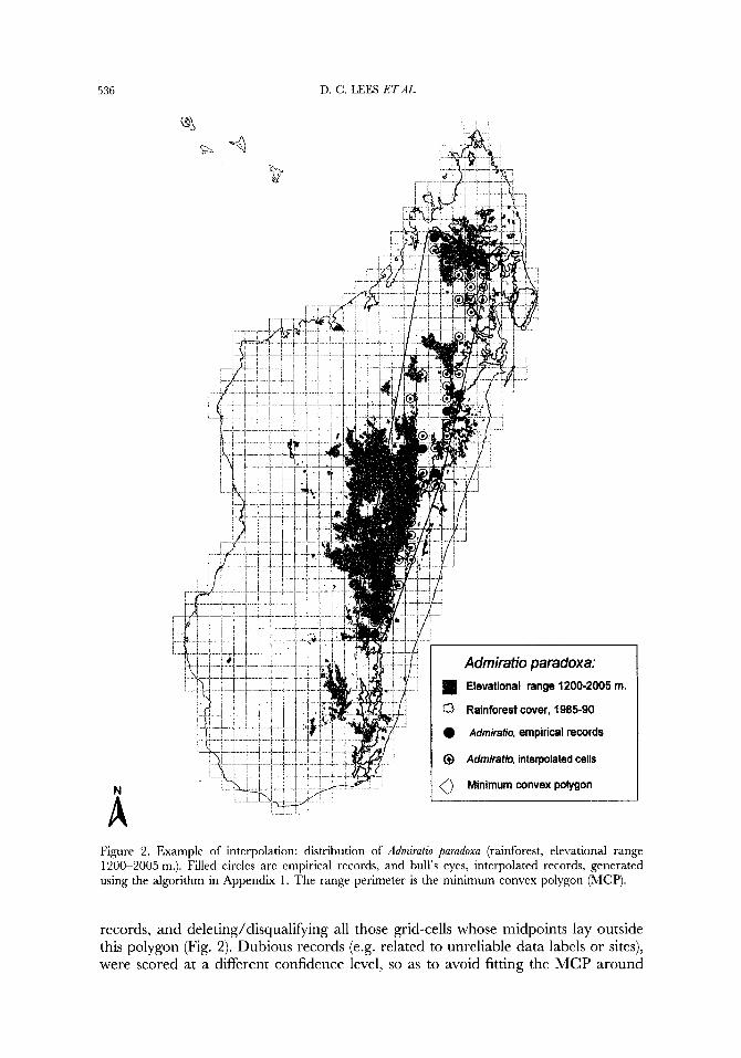
Species richness patterns have been analysed using WORLDMAP iv WINDOWS (Williams, 1998) on a quarter degree grid containing 93 1 grid-cells for Madagascar, each approximately 27 x 27 km. This scale is fine enough to be highly sensitive to biogeographic patterns, but coarse enough for most rainforest biome grid-cells to contain one or more empirical records. These grid-cells vary in planar area from about 697.5 km' at 25.5"s to about 756 km' at 12"s. Species richness was calculated by WORLDMAP as the raw species count per grid-cell. Data records were coded separately as empirical or interpolated (e.g. Fig. 2).
Inteqolation
To make best use of the data available in the face of highly uneven sampling effort, some data treatment is required. In this study, because sufficiently detailed environmental models were not readily available for adopting an extrapolative or probabilistic approach (e.g. Nix, 1986; Nicholls, 1989; Busby, 199 1; Carpenter, Gillison & Winter, 1993; Colwell & Coddington, 1994; Franklin, 1995; Augustin, Mugglestone & Buckland, 1996), ranges were interpolated using a simple method. Interpolation of species' ranges compensates for unevenness in sample effort so as to clarify patterns of species richness (e.g. Williams et al., 1996). How accurately it does this depends not only on the modelling techniques used but on subsequent ground-truthing and iterative refinements of the model. In interpolation, range continuity is assumed between recorded limits (with the exceptions noted below); however, range overlap of two or more species here by no means implies sympatry at a spatial scale finer than a quarter of a degree, in ecological space or time (see Gaston, 1996).
An algorithmic method was developed to automate interpolation (Appendix 2). For bandwise, one-dimensional ( = ' 1-D') species richness (here using either latitudinal or elevational gradients), interpolation was simply carried out by assuming contiguity for each species between reliable empirical range limits. For the geographic, two- dimensional ( = '2-D') approach (using both latitudinal and longitudinal gradients), a more sophisticated interpolation method was used which depended on comparison of both species and grid-cell elevational ranges and habitat codes (Appendix 1).
To carry out the 2-D interpolation for each species, these two biological parameters, elevational range and habitat type(s), were determined from sampling records, if available, or inferred from locality details (e.g. those given by Viette, 1991), if unknown. Thus, for primary forest restricted species, only cells containing re- cognizable extant primary forest fragments were scored even if appropriate map elevational range data were available (Fig. 2). The range was then truncated using a convex hull or minimum convex polygon (MCP: Rapoport, 1982; Agassiz et al., 1994; Gaston, 1996) fitted around the vertices of all reliable empirical grid-cell
536 D. C. LEES ETAL.
A Figure 2. Example of interpolation: distribution of Admiratio parudoxa (rainforest, elevational range 1200-2005 m.). Filled circles are empirical records, and bull's eyes, interpolated records, generated using the algorithm in Appendix 1. The range perimeter is the minimum convex polygon (MCP).
records, and deleting/disqualifying all those grid-cells whose midpoints lay outside this polygon (Fig. 2). Dubious records (e.g. related to unreliable data labels or sites), were scored at a different confidence level, so as to avoid fitting the MCP around
SPECIES RICHNESS G U D I E N T S 537
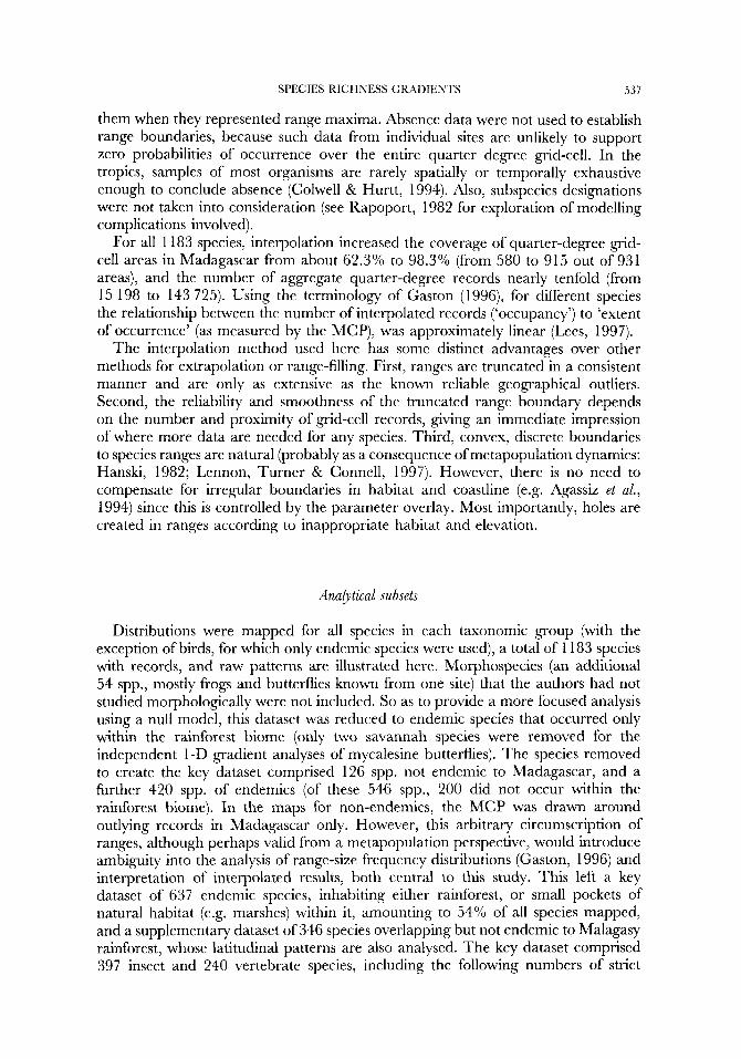
them when they represented range maxima. Absence data were not used to establish range boundaries, because such data from individual sites are unlikely to support zero probabilities of occurrence over the entire quarter degree grid-cell. In the tropics, samples of most organisms are rarely spatially or temporally exhaustive enough to conclude absence (Colwell & Hurtt, 1994). Also, subspecies designations were not taken into consideration (see Rapoport, 1982 for exploration of modelling complications involved).
For all 1 183 species, interpolation increased the coverage of quarter-degree grid- cell areas in Madagascar from about 62.3% to 98.3% (from 580 to 915 out of 931 areas), and the number of aggregate quarter-degree records nearly tenfold (from 15 198 to 143 725). Using the terminology of Gaston (1996), for different species the relationship between the number of interpolated records (‘occupancy’) to ‘extent of occurrence’ (as measured by the MCP), was approximately linear (Lees, 1997).
The interpolation method used here has some distinct advantages over other methods for extrapolation or range-filling. First, ranges are truncated in a consistent manner and are only as extensive as the known reliable geographical outliers. Second, the reliability and smoothness of the truncated range boundary depends on the number and proximity of grid-cell records, giving an immediate impression of where more data are needed for any species. Third, convex, discrete boundaries to species ranges are natural (probably as a consequence of metapopulation dynamics: Hanski, 1982; Lennon, Turner & Connell, 1997). However, there is no need to compensate for irregular boundaries in habitat and coastline (e.g. Agassiz et al., 1994) since this is controlled by the parameter overlay. Most importantly, holes are created in ranges according to inappropriate habitat and elevation.
Anahtical subsets
Distributions were mapped for all species in each taxonomic group (with the exception of birds, for which only endemic species were used), a total of 1 183 species with records, and raw patterns are illustrated here. Morphospecies (an additional 54 spp., mostly frogs and butterflies known from one site) that the authors had not studied morphologically were not included. So as to provide a more focused analysis using a null model, this dataset was reduced to endemic species that occurred only within the rainforest biome (only two savannah species were removed for the independent 1 -D gradient analyses of mycalesine butterflies). The species removed to create the key dataset comprised 126 spp. not endemic to Madagascar, and a further 420 spp. of endemics (of these 546 spp., 200 did not occur within the rainforest biome). In the maps for non-endemics, the MCP was drawn around outlying records in Madagascar only. However, this arbitrary circumscription of ranges, although perhaps valid from a metapopulation perspective, would introduce ambiguity into the analysis of range-size frequency distributions (Gaston, 1996) and interpretation of interpolated results, both central to this study. This left a key dataset of 637 endemic species, inhabiting either rainforest, or small pockets of natural habitat (e.g. marshes) within it, amounting to 54% of all species mapped, and a supplementary dataset of 346 species overlapping but not endemic to Malagasy rainforest, whose latitudinal patterns are also analysed. The key dataset comprised 397 insect and 240 vertebrate species, including the following numbers of strict
538 D. C. LEES ETA4L.
rainforest endemic species in each group: butterflies (1 45), frogs (1 26), enariine beetles (87), cicindelid beetles (85), ctenuchiine moths (80), birds (36), chameleons (35), tenrecs (19), rodents (15) and lemurs (9). Because counts of empirical species richness are extremely uneven for most if not all of these groups in Madagascar for sampling reasons alone, this paper focuses on species richness patterns shown by interpolated data, which makes optimal use of the empirical data.
Range-size rarip classes
All the rainforest endemics were classified by range size. For convenience hereafter, the terms 'widespread' and harrow-spread' are applied, in the precise and gen- eralisable sense of subsets of an array of species which occupy more than or equal to half, or less than or equal to half the total maximum span of a given domain, respectively. To examine in detail the potential of geometric constraints to explain the observed latitudinal patterns, the pool of all 637 rainforest species was divided into four range size classes spanning the 13 degrees (52 latitudinal bands) that approximately span the extreme limits of the rainforest biome (12.25"s and 25.25"S), and are also only marginally short of the 'hard' marine boundaries of Madagascar. For the l-D case, discrete range sizes estimated by subtraction of grid-cell latitudinal centroids were classified in the following classes each encompassing 13 quarter- degree latitudinal bands: 0-3', 3.25-6.25", 6.5-9.5" and 9.75-1 2.75" (and also a single latitudinal band class, 0-0.25"). For the 2-D case, 48 quarter-degree bands were used (due to the northern rainforest gap shown in Fig. 1, that is a more appropriate span), and species reclassified accordingly (0-2.75", 3-5.75", 6-8.75" and 9-1 1.75"). The cells in the analytical spans were scaled between 0 and 1 using the following correction: x= (i-0.5)/N, where x is the value assigned to the centroid of grid-cell i (from 1 . . .N), and N is the number of grid-cells in the span. This correction distributes values of x evenly over even small numbers of cells (this is here the case for longitudinal spans), whilst avoiding application of logarithmic equations to zero. For mycalesines, latitudinal range analyses used the 13 degree span, whilst 0 and 2 100 m. were taken as the appropriate elevational limits for the group.
For l-D comparisons against the null model, each quarter-degree presence value of each species' interpolated range was summed within the allotted classes to generate the observed l-D values, whilst the null equations, described in results and derived in Appendix 2, were used to calculate expected values. The Mann-Whitney U-test for tied variates where 020 (Sokal & Rohlf, 1981) was the non-parametric statistic applied to test for significant departure from the null model in the central tendency (median) of a proportional species richness distribution for each quarter-degree latitudinal band. The two-sample Kolmogorov-Smirnov statistic, more sensitive to differences in shape of the overall distribution, was used to test for goodness of fit. For 2-D comparisons against the null model, species richness counts for each grid- cell were simply exported from WORLDMAP and referenced to latitude, filtered using a list of rainforest cells, and compared with 2-D predictions (derived as explained in the analytical results section), including for the top scoring (hotspot) values within each latitudinal band.
SPECIES RICHNESS GRADIENTS 539
Sensitivip analyses
Interpolation already provides substantial smoothing for the irregularity of sample effort in Madagascar. However, mid-gradient species richness could still be promoted in two main ways. Firstly, there is a sampling problem both at local and regional levels. Very localized endemics are over-recorded (and potentially over-split) compared with nearby grid-cells, especially because the principal capital-coast road and railway routes occur at c. 18-19"s. Also, well-sampled areas, in particular Ptrinet- Analamazaotra/Mantady (the 'Ptrinet grid-cell', c. 19OS) are likely to constitute the recorded range extreme for more widespread species which do not quite reach the next relatively well sampled point, 2.25 degrees south in the Fianarantsoa/ Ranomafana region, or 1.25 degrees north in the Zahamena region (Fig. 1). Secondly, area differences at different latitudes might also influence species richness: where land is widest longitudinally, species richness for that latitudinal band might be enhanced by factors such as greater aggregate habitat diversity or greater freedom of range overlap.
To assess the effect of these potential sampling biases, stringent tests were imposed. To test the effect of over-sampling, empirical records for the Ptrinet grid-cell, which for most groups is the most heavily sampled grid-cell, were eliminated from the dataset of 637 rainforest endemics. Interpolation was then performed without these empirical records. The resulting score for the Ptrinet grid-cell was thus entirely reliant on the results of interpolation, thereby eliminating the effects of relative over- sampling. To test for one possible effect of area, ranges where the longitudinally aligned axis exceeded the latitudinal axis were removed from a copy of the dataset, eliminating a major potential component of any surplus of species richness where rainforest was broader.
flu11 model
To provide an analytical alternative to the randomization procedure in Colwell & Hurtt (1994), a probabilistic approach was employed. As in Colwell & Hurtt, this takes account of continuous functions of both range size and range position, a shortcoming of the discrete painvise range overlap probability model of Pielou (1977) (although see modifications by Dale, 1986, 1988; Sugihara, 1986). However, the purpose of the present model is to evaluate species richness, not degree of overlap. In contrast to the binomial probability model of Willig & Lyons (1 998), which does attempt to evaluate levels of species richness, this model does not implicitly assume that the points defining range limits are independent.
For the most basic 1-D model, the geographic span of a latitudinal or elevational gradient was represented along the x-axis, with any position x (in the range 0-1) representing a hypothetical species sampling transect. The y-axis was used to represent any species range of size r, also varying from 0 to 1 as a function of x for each species (Fig. 3A). T o facilitate comparison with the four Monte Carlo models of Colwell & Hurtt (1994), the range midpoint constraint envelope is indicated in Figure 3A. This model is in fact the converse of Colwell & Hurtt Model 3 (that randomizes range size given midpoint). The basic assumptions of the simplest version of this model [with possible refinements noted] are:
(1) Species spans were unfragmented [gaps in species ranges were in fact included
540
A 1
r
0.75
0.5
0.25
0
\ ln(0.25/x)
x ln(2)
x ln(0.7510.5)
0
B
0.25
X - 0.25
K \ ln(0.5/x)
+ 0.25- X
ln(1/0.75)- 0.25
0.25 1.5 '0.75 X
SPECIES RICHNESS GRADIENTS 54 I
for the 2-D case; their existence would reduce the level of species richness at some positions of x, so that the 1-D model can be seen as providing an upper bound to species richness].
(2) Both boundaries of the gradient span along which the species were distributed were of the ‘hard’ type (Colwell & Hurtt, 1994). Accordingly, the probability of occurrence of an extreme position of a range infinitesimally beyond, and also at, a hard boundary was taken to be zero. [Organisms such as sea birds and migrants were not included in the analytical dataset, and so this assumption seems a reasonable approximation for most terrestrial endemics].
(3) Species ranges were distributed according to a uniform distribution both for placement along the gradient and for size of range (both varying from 0 to 1). Specifically, conditional on a given range size of a species, the midpoints or endpoints (in this model, it makes no difference which is chosen) were uniformly distributed across permitted values (in the case of midpoints, the midpoint constraint envelope shown in Fig. 3A). [In the simplest version of the model, the range size frequency distribution was assumed to be uniform; refinements of the model using analytical equations for range size classes allow approximations to more complex range size frequency distributions.]
RESUI.‘I’S
Analytical equations
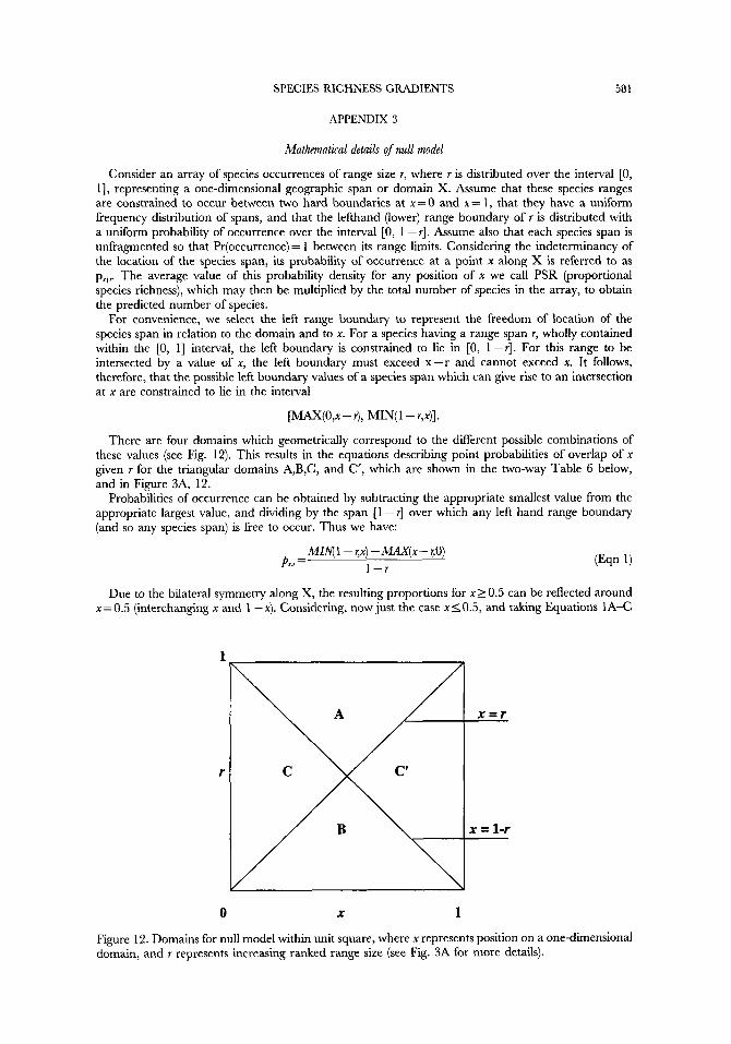
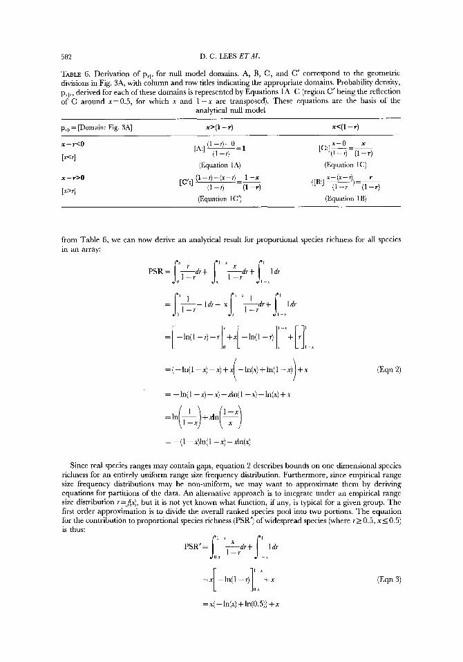
The geometric consequences of the null model assumptions for the I-D case are illustrated in Figure 3, including Equations 1A-C (derived in Appendix 2) for probabilities of occurrence for a given range size and gradient position (p.,.) for each of the four triangular domains. These equations are the building blocks for
Figure 3. (A) Null model. Probability density, p t , , is represented as graduated shading for each of four complementary triangular domains A, B, C and C’ (solid white lines) of a plot of r, species range size, against x , sampling position on a geographic domain X. This is a two-dimensional representation of a uniform distribution of species range midpoints along the unit line, ranges being bounded absolutely by X=O and X = 1. As examples, the horizontal black bars represent the leftmost possible limits of species spans measuring 0.25 and 0.75 of the geographic domain, and their midpoints fall on the isoceles triangular constraint envelope indicated by the dashed lines. Ranges of widespread species ( r 2 0.5) must always mutually overlap and are always intersected by a given value of x (p = 1) within domain A. Ranges of narrow-spread species ( r l 0.5) have a maximal probability of intersection by x equal to the average probability of intersection by x (this equals r) divided by the freedom of location of any species range (1 -r), within domain B. Probability of intersection by x in domains C and C’ is proportional to x or 1 - x , increasing linearly up to either of the two regions of maximal probability of intersection for any value of r (A and B) whose boundaries are x = r or x = ( l - 3 . Integration of these probability densities produces a quasi-parabolic curve representing proportional species richness, whose peak value and shape depends on the scaling of r (the range size frequency distribution of the species assemblage). (B) Analytical formulae describing contribution to proportional species richness (PSR’) for 12 independent domains of the left hand side of 3(A) derived as for two classes in Appendix 2, here for four equal-span partitions of ranked range size. The formulae sum to those applicable for smaller numbers of classes; formulae for the right hand side may be obtained by transposing x and 1 - x .
542 D. C. LEES ETAL.
this analytical treatment detailed in Appendix 2. Equations given here are numbered as in Appendix 2.
Equation 2 (derived in Appendix 2) summarizes these equations by describing proportional species richness (PSR) under the uniform distribution for any point x on a gradient from x = O to x=0 .5 (although unnecessary in this case, in general values from x = O . 5 to x = 1 are obtained by transposing x and 1 - x ) :
PSR = - (1 - x)ln( 1 - x) - xln(x) (Eqn 2) This equation applies only to the simplest case where the range size frequency distribution is uniform. Then the number of widespread species equals the number of narrow-spread species, i.e. S, = SN, when proportional species richness evaluates to ln(2) (% 0.6931) at x=0.5.
Further analytical equations for different classes of range size, on which the statistical comparisons of empirical species richness curves are based, are itemised in Appendix 2. For the contribution to proportional species richness (PSR') of widespread species,
PSR'=xln - + x (O:)
whereas for narrow-spread species,
PSR' = x l n ( g ) + ln(&) - x
These individual null equations allow evaluation of empirical species richness curves obtained for mutually exclusive range size classes, and also can be input into an equation that more accurately estimates empirical ranked range size distributions as the number of classes increases. Thus,
where C ,n are mutually exclusive range size classes, P is the proportion of species in class Cl,, . , , andfcl.,,n (x ) is the function of x that describes the contribution to proportional species richness (PSR') of that class.
A special case of Equation 7 is given by a null equation for the 2-class approximation to hotspot species richness (Sma), where x = 0.5,
S m a % S ( 9 + ((1 - \1/)(21n(2) - 1))) (Eqn 9) where S is the total number of species, and + is the proportion of widespread species. Note that this can also be expressed by:
s,, % s, + (21n(2) - 1 ) s N % s, + 0.3863SN (Eqn 9 4 where S, denotes the total of widespread species, and SN denotes the total of narrow- spread species. The coefficient for SN is simply the average probability density of
SPECIES RICHNESS GRADIENTS 543
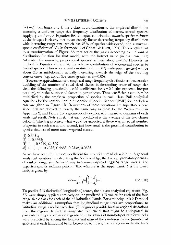
( r / 1 - r) from limits a to b, the 2-class approximation to the empirical distribution assuming a uniform range size frequency distribution of narrow-spread species. Applying the form of Equation 9A, an equal contribution towards species richness at the hotspot is clearly met by an exactly linear decreasing frequency distribution with increasing range size, which has 25% of species widespread, and a narrow- spread coefficient of 1 /3 (as for model 2 of Colwell & Hurtt, 1994). This is equivalent to a transformation of Figure 3A that scales the y-axis according to the ranked distribution function for that model, with the hotspot value (in that case, 0.5) calculated by summing proportional species richness along x = 0.5. However, as implicit in Equations 3 and 4, the relative contribution of widespread species to overall species richness for a uniform distribution (50% widespread species) will be about 2.6 at mid-domain, actually increasing towards the edge of the resulting convex curve (e.g. about five times greater at x=0.05).
Successive approximations to empirical range frequency distributions for successive doubling of the number of equal sized classes in descending order of range size yield the following practically useful coefficients for x = 0.5 (the expected hotspot position), with the number of classes in parentheses. These coefficients can then be multiplied by the empirical proportion of species in each class. Full analytical equations for the contribution to proportional species richness (PSR') for the 4-class case are given in Figure 3B. Derivations of these equations are superfluous here since they are derived in exactly the same way as those for the 2-class result in Appendix 2, and Figure 3B is geometrically explicit with regard to domains of each analytical result. Notice first, that each coefficient is the average of the two classes below it (which is precisely what would be expected if there was an equal number of species in each class), and second, just how small is the potential contribution to species richness of more narrow-spread classes.
As we have seen, the hotspot coefficient for any widespread class is one. A general analytical equation for calculating the coefficient kNs, the average probability density of ranked range size between any two narrow-spread ( 6 0 . 5 ) range sizes at the expected species richness peak x=0.5, where a is the upper limit, b is the lower limit, is given by:
To predict 2-D (latitudinal-longitudinal) scores, the 4-class analytical equations (Fig. 3B) were simply applied iteratively on the predicted 1-D values for each of the four range size classes for each of the 52 latitudinal bands. For simplicity, this 2-D model makes an additional assumption that longitudinal range sizes are proportional to latitudinal range sizes for each class. (This ignores possible local or regional deviations from the regional latitudinal range size frequencies that might be anticipated, in particular along the elevational gradient.) The values of non-hotspot rainforest cells were predicted by scaling the longitudinal span of the rainforest biome (number of grid-cells at each latitudinal band) between 0 to 1 using the correction in the methods
541
Fipre 4. One-dimensional range size distributions. A, ranked latitudinal (front) and elevational (back) range size distributions for mycalesines. B -F, range size frequency distributions. B {from back to front): all 1 1 8 3 spp. mapped; 879 rainforest species, and 637 strict rainforest endemics. C-F subsets (including all rainforest-occurring species) for ten focal groups. C, mycalesine buttedies (front. 65 spp.), contrasted
SPF,ClES RICHNESS GRADIENTS
--\-
545
" I" " i2 ' 3 ' 4 '
with other butterflies (back, 144 spp.). D, chameleons (47 spp.), frogs (156 spp.) and birds (75 spp.). E, cicindelid (1 33 spp.) and enariine ( 1 03 spp.) beetles and ctenuchiine moths (94 spp.). F, lemurs (22 spp.), tenrecs (23 spp.) and rodents (1 3 spp.). Note the very differently skewed, or even bimodal, range size frequency patterns for different groups.
546 D. C . LEES ETAL.
section, and reapplying the analytical equations to the l-D score for each case. A 2-D predictive map is the result (Fig. 84). Conveniently, it is not necessary to take into account this longitudinal span in order to predict the 2-D species richness peak.
Range size distributions of the groups mapped
Analysing range size distributions is an essential first step in examining how biological constraints interact with geometric ones. For example, for a linear ranked range distribution (and a uniform range size frequency distribution), Equation 2 would serve as an adequate l-D geometric description. In fact, Madagascan mycalesine butterflies do exhibit a somewhat linear ranked l-D range size distribution both for latitude and elevation (Fig. 4A), although for latitude there is a larger number of species with very small ranges, as reflected in the left hand side of the range size frequency distribution in Figure 4C. Figure 4B shows l-D range size frequency distributions for all animals mapped (1 183 spp.), compared with all rainforest-occurring species (879 spp.) and the analytical dataset of 637 spp. The strict rainforest endemic dataset differs in lacking a large right hand modal class to the range size distribution, since species not endemic to mainland Madagascar are lacking (note that the generally larger range sizes for such species are inevitably underestimated). However, all sets exhibit a highly pronounced smallest range size class. For comparative purposes, range size frequency distributions for individual groups here show all rainforest-occurring species, because of the small number of strict rainforest endemics in some groups.
A classic right-skewed ‘hollow curve’ (this term denotes any concave curve: see e.g. Willis, 1922; Anderson, 1985) is shown by no one group, and some groups, such as tenrecs (Fig. 4F), even lack the small range size modal class. Birds (Fig. 4D) actually show the mirror pattern. Indeed, there are marked differences between groups. Mycalesines contrast greatly with other butterflies, even though these comprise other large endemic radiations (such as Strubenu, ypthimine Satyrinae), but the non-mycalesine butterflies also include a high proportion of non-endemic species. Groups with a high proportion of endemic species (Table l), such as mycalesines (Fig. 4C), frogs and chameleons (Fig. 4D), ctenuchiine moths, and enariine and cicindelid beetles (Fig. 4E), show a moderately even distribution of range sizes, but with a greatly inflated one degree grid-cell peak (in fact, most of this peak is concentrated within one quarter degree latitudinal band). However, this pattern is not invariably the case, since the rainforest-occurring birds mapped, as well as tenrecs and lemurs, are all Madagascar endemics, and the rodents predominantly comprise the large radiation of Nesomyinae. The contrasting range size distributions of these homoiotherms may well reflect higher body size and mobility in relation to spatial scale, factors not examined here.
The large narrowly endemic classes for many groups may at least partly be artifacts both of oversplitting and underestimation of range size. The relative contribution of these two factors is unclear. The analytical equations relate such range size frequency distributions to species richness curves. Thus, the predicted proportional contribution of the smallest grid-cell class to the hotspot is minimal: only about 0.0406 in the case of a one degree band, or about 0.0097 in the case of a quarter degree band, for a 13 degree span (Equation 10). Thus, although the empirical ratio here of narrow-spread to widespread strict rainforest endemics of
SPECIES RICHNESS GRADIENTS 547
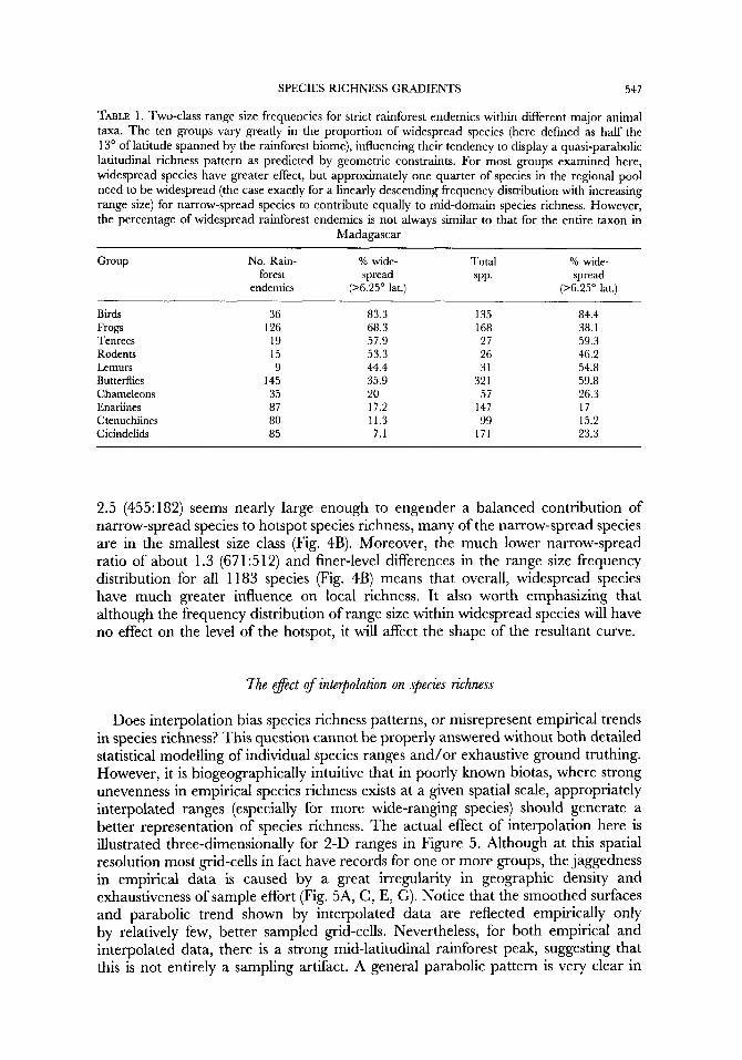
TABLE 1. Two-class range size frequencies for strict rainforest endemics within different major animal taxa. The ten groups vary greatly in the proportion of widespread species (here defined as half the 1 3" of latitude spanned by the rainforest biome), influencing their tendency to display a quasi-parabolic latitudinal richness pattern as predicted by geometric constraints. For most groups examined here, widespread species have greater effect, but approximately one quarter of species in the regional pool need to be widespread (the case exactly for a linearly descending frequency distribution with increasing range size) for narrow-spread species to contribute equally to mid-domain species richness. However, the percentage of widespread rainforest endemics is not always similar to that for the entire taxon in
Madagascar
Group No. Rain- YO wide- Total % wide- forest spread SPP. spread
2.5 (455:182) seems nearly large enough to engender a balanced contribution of narrow-spread species to hotspot species richness, many of the narrow-spread species are in the smallest size class (Fig. 4B). Moreover, the much lower narrow-spread ratio of about 1.3 (67 1 :5 12) and finer-level differences in the range size frequency distribution for all 1183 species (Fig. 4B) means that overall, widespread species have much greater influence on local richness. It also worth emphasizing that although the frequency distribution of range size within widespread species will have no effect on the level of the hotspot, it will affect the shape of the resultant curve.
irhe efect of interpolation on species richness
Does interpolation bias species richness patterns, or misrepresent empirical trends in species richness? This question cannot be properly answered without both detailed statistical modelling of individual species ranges and/or exhaustive ground truthing. However, it is biogeographically intuitive that in poorly known biotas, where strong unevenness in empirical species richness exists at a given spatial scale, appropriately interpolated ranges (especially for more wide-ranging species) should generate a better representation of species richness. The actual effect of interpolation here is illustrated three-dimensionally for 2-D ranges in Figure 5. Although at this spatial resolution most grid-cells in fact have records for one or more groups, the jaggedness in empirical data is caused by a great irregularity in geographic density and exhaustiveness of sample effort (Fig. 5A, C, E, G). Notice that the smoothed surfaces and parabolic trend shown by interpolated data are reflected empirically only by relatively few, better sampled grid-cells. Nevertheless, for both empirical and interpolated data, there is a strong mid-latitudinal rainforest peak, suggesting that this is not entirely a sampling artifact. A general parabolic pattern is very clear in
Figure 5. Three dimensional species richness patterns revealing visually the effect of interpolation (right, B,D,F,H) on empirical records (left, A,C,E,G). The extreme irregularity in sample effort for empirical records is apparent (compare A with B, showing all 1183 species mapped), but a hotspot is also apparent at mid latitudes of the rainforest biome for empirical data. Interpolation compensates for sampling gaps and thus more accurately reflects patterns in species richness, which emerge as a domed shape, particularly for 983 rainforest occurring species (compare D with C). In contrast, the
SPECIES RICHNESS GRADIENTS 549
TABLE 2. Position of hotspots for the major animal taxa. Data indicate species richness of interpolated Pkrinet grid-cell relative to warmest hotspot. Hotspot(s) are indicated 1-dimensionally as latitude, direction relative to 19"S, italicized where they coincide with the Pkrinet grid-cell, the case for six groups. The skew of the hotspot relative to this grid-cell is indicated qualitatively here, in direction
and by ratio; ns =no skew (qualitative). *Empirical data
interpolated graphs for rainforest species (Fig. 5B, D). However, for the 200 non- rainforest species, a somewhat bimodal pattern emerges (with the largest hotspot at the latitude of Ankarafantsika, 16"s: Fig. 5F). Narrow-spread animals (67 1 spp.) exhibit a quite irregular, north-skewed pattern, a trend smoothed only to some degree by interpolation (Fig. 5G, H). Qualitatively at least, interpolation does not apparently alter the underlying trend shown by empirical results, although it may sometimes change the position of the hotspots (Tables 2, 3).
Species richness gradients f o r mycalesines
When mycalesines are ranked by latitudinal range (Fig. 6) a maximum is shown at about the latitude of the Pkrinet reserve, 19"s. The domed curve for one dimensional species richness is not significantly different in central tendency (Mann- Whitney test statistic, mw = 1.53; DO. 1) from a bounded uniform distribution adjusted for 4 empirical classes, although the distribution is somewhat irregular (Lees, 1996). Partitioning into widespread and narrow-spread species shows that the profile for widespread species is clearly much smoother, and is also not significantly different in central tendency from the null model (mw=0.165, -0.8). Only the narrow-spread species show a significant departure from the bounded uniform distribution (mw = 3.263, P<0.01), and are largely responsible, considering their high proportion (2. l), for irregularities in the overall profile.
more irregular pattern that emerges when the 200 non-rainforest species are interpolated (compare F with E) reflects the highly fragmented nature of non rainforest habitats. Any influence on the overall pattern (A,B) of the irrepular, asymmetric distribution exhibited by the 67 1 narrow-spread animals (G,H) is largely masked by a disproportionate influence on overall species richness of widespread sprcies.
550 D. C. LEES E T A L .
TABLE 3. Position of hotspots for 22 different faunal groups, mostly radiations, ranked in order of species richness for each major group. Direction relative to 19"s. Relative species richness of Ptrinet grid-cell to hotpot cell(s) in final column. As in Table 2, results indicate qualitatively a skewed distribution relative to the Pkrinet grid-cell (italicized), but more groups show an unambiguously northern skew (12) than show a southern skew (3), relative to mid latitudes. Smaller groups are more likely to exhibit an idiosyncratic species richness distribution. However, the mid-latitudinal 1 O band comprising the Pkrinet grid-cell includes a hotspot for 12 of the groups, whereas no other one degree band includes a hotspot for more than seven taxa. $Evidence exists for paraphyly or polyphyly in relation to extant non-Malagasy faunas. *Interpolated and empirical. #Only empirical. ^Nan-rainforest.
One-dimensional species richness of mycalesine butterflies along the elevational gradient also shows a hotspot near mid-gradient, although here at the upper part of the elevational range of the Ptrinet grid-cell (Fig. 7). Mycalesine elevational species richness exhibits evidence for the mid-elevationally humped pattern (Rahbek, 1995), most clearly for widespread species, although overall, the pattern is clearly bimodal, a pattern caused by narrow-spread species. Furthermore, the species richness gradient is strongly asymmetric, with species richness considerably higher from 0 to 500 m. than from 1500 to 2000 m. Accordingly, all curves in Figure 7 differ significantly in central tendency from the null model (all species: mw = 3.529, P<O.OOl; widespread: mw = 3.047; P<O.Ol; narrow-spread: mw = 1.943; P<0.05).
SPECIES RICHNESS GRADIENTS 55 1
Overall species richness gradients for dgerent taxa
Is a mid-gradient diversity peak typical of other rainforest taxa? This question is examined qualitatively here for 2-D ranges within different groups, for the latitudinal gradient (Fig. 8). Furthermore, all species mapped (Fig. 8A, B), are compared with the 637 rainforest species (Fig. 8P), and the 546 species either not exclusive to rainforest or non-regionally endemic, divided into humid forest and drier habitat classes (Fig. 8N, 0). The much sharper biogeographic signal resulting from in- terpolated ranges is again shown for all taxa in Figure 8B (compare with Fig. 8A). The broadest pattern is a west to east trending (longitudinal) gradient in species richness per grid-cell, maximal within the rainforest biome. Correspondence between species diversity and gradients in topographic complexity, rainforest cover, and moisture at a cross-biome level, is widely acknowledged (e.g. O'Brien, 1983). However, even in this respect, taxa clearly vary. Mycalesine butterflies (Fig. 8D), with one savannah-restricted exception, all occur either in rainforest, deciduous forests transitional to rainforest, or at their margins, whereas birds (Fig. 8M) and chameleons (Fig. 81) are more diverse in their habitat preferences. Within the (for ail major groups much richer) rainforest biome, species richness increases towards mid-latitudes and elevations, both overall (Figs 5A, B and 8A, B) and for the 346 rainforest-occurring non-endemic species (Fig. 8N). The most symmetrically humped pattern, though, is shown for the rainforest endemic subset (Fig. 8P). The non- humid forest species set of 200 species (Figs 5F, 80), show a quite different, much patchier species richness pattern, with a hotspot in north western deciduous forests at about 16"s.
In sharp contrast to some temperate zone studies (e.g. Prendergast et al., 1993), there is a strong congruence between interpolated species richness maps for all the different groups, with some groups such as enariine beetles (Fig. 8C), mycalesines (Fig. 8D), other butterflies (Fig. 8E), and frogs (Fig. 8F) particularly closely matching the trend and hotspot position of the entire dataset (Tables 2, 3). Apparent for some groups is a northwards skew (e.g. for ctenuchiine moths: Fig. 85 and cicindelid beetles: Fig. 8K) or southwards tendency (e.g. for tenrecs: Fig. 8H), highlighted by the position of the species richness hotspot(s) (Fig. 8, Tables 2, 3). Lemurs (Fig. 8L) even show a bimodal distribution.
A species richness hotspot for 1-D and 2-D interpolated range maps (and usually also empirical ones) often coincides in position with the PCrinet grid-cell (1 8'45'-19"OO'S, 48'1 5'-48'30'E): Tables 2, 3. A mid-domain peak is exhibited by mycalesines (Figs 6, 8D), all buttedies other than mycalesines (Fig. 8E), frogs (Fig. 8F), enariines (Fig. 8C), rodents (Fig. 8G), tenrecs (Fig. 8H), chameleons (Fig. 81), birds (Fig. 8M), as well as a number of other substantial taxonomic subgroups within the dataset. Hotspot positions, however, need to be interpreted with great caution (Palmer & White, 1994). Even considering one spatial scale alone, because in- terpolated range richness may be relatively flat (as for some groups especially near mid-latitudinal span), the position(s) may be sensitive to a change in very few species, even for species-rich taxa. For mycalesines (all species), for example, 1-D ranges show only a hotspot at Pkrinet (Fig. 6), but for 2-D ranges the southern Ranomafana peak is equally rich (Fig. 8D). In particular, the apparent consistency for many groups of a hotspot position around PCrinet may in part be a result of over-sampling in or adjacent to this relatively well-worked grid-cell. Nevertheless, despite marked differences in the regional distribution of sample effort for different focal taxa, species
552 D. C. LEES E T A L
becies <= 25"s
Ihr?o&h 138 H.nasi. 25
I O B
12.5% =>
W
+ALL (Ob8.- 65 WP.) ALL (anaiytical-4)
- WSP (analytical-2) -WSP (obs.-21 qp . )
l i 24 22 20 Latitudk?(oSouth)'6
14
SPECIES RICHNESS GR4DIENTS 553
richness hotspot(s) occur within a latitudinal band of 18.25-19's for seven of the ten focal groups mapped (Table 2; tiger beetles, ctenuchiine moths and lemurs are the exceptions). Eleven of 22 groups with 1 1 or more species (most evolutionary radiations) also peak in this area, accounting in all for 678 species (Table 3). In contrast, no other 1" latitudinal band contains a maximal hotspot for more than seven of these groups. Notice that smaller taxonomic subsets more often show differences in hotspot position (Table 3), with some taxa even exhibiting hotspots outside the rainforest biome. Nevertheless, their 2-D aggregate hotspot still coincides with the Ptrinet grid-cell for both empirical and interpolated data. Thus, a more symmetrical domed pattern emerges from taxonomically idiosyncratic distributions.
Mid-gradient sample efort sensitivig anabses
Could the common mid-gradient diversity peaks in mycalesines and other Ma- dagascan animals be an artifact of heavy mid-gradient sampling, however? For rigorous evaluation of the influence of over-sampling on the Ptrinet 'hotspot' using a sensitivity analysis, strict rainforest endemics have been analysed here. Global removal of the empirical records for the Ptrinet grid-cell affected the ranges of 69 out of these 637 species (Fig. 9A). Eight of these species were widespread, 56 and narrow range sizes (between 0.5 and seven degrees), and five were eliminated as single grid-cell endemics. In fact, the result was to bring the Ptrinet grid-cell's richness score down to the adjusted level of the adjacent cells. Removal of the Ptrinet grid-cell records had no significant effect on the central tendency or a 4th order polynomial fitted through the points (mw = 0.0787; -0.9), with a similar result for the original points (mw = 0.135, -0.8). So, although some local relative over-sampling was apparent, the Ptrinet grid-cell records did not significantly promote the medially symmetric pattern.
Environmental gradients
The most salient feature of the latitudinal species richness curves for endemic rainforest species is that they do not generally significantly differ in central tendency and shape from the convex curves generated by the null model. However, could this type of curve alternatively reflect a congruent response of taxa to unusual environmental conditions in Madagascar? If this is the case, environmental variables favourable to species diversity should exhibit a similar shape, as well as be significantly correlated with species richness. Particularly strong candidate factors are surface area and energy.
Figure 6. One-dimensional latitudinal range sizes of mycalesines (all spp.). Species are ranked by latitudinal range size, assuming contiguous ranges, and the resulting profiles for 23 widespread (WSP, middle curve) and 44 narrow-spread (NSP, lower curve) species are compared against 2-class analytical equations, and all 65 spp. (ALL, top curve) against 4-class equations for the bounded uniform distribution. These classes correspond to the divisions of the list of species into two and four equal- span partitions of ranked range size. The shaded mid-gradient line marks the latitude of the Pkrinet grid-cell. Note the relatively smoother distribution and closer fit to the null model for the widespread species.
Environmental gradients in Madagascar are illustrated in Figures LOA-L, and in relevant cases contrasted with measures for grid-cells just within the original rainforest biome (open circles). Widespread and narrow-spread species are also compared in their response to these factors (Table 4). Here, since significance levels are potentially inflated by spatial autocorrelation, only non-significance can be relied upon, but correlation coefficients do retain some comparative value (Table 4). Considering now only rainforest grid-cells, all gradients related to energy increase from the southern to the northern limit of the rainforest biome (Fig. lo), and involve differing correlations with species richness. For instance, Spearman coefficients are positive for mean monthly rainfall (Fig. 1 OB; although non-significant for widespread species) and hydric credit (Fig. lOC), but are negative for mean annual temperature (Fig. 1 OA), solar radiation (Fig. 1 OE), and potential evapotranspiration or PET (Fig. 1 OD). Furthermore, productivity (often expressed as biomass) has sometimes been characterized as having a hump-shaped relationship with species richness (e.g. Rosenzweig, 1992). However, northwards increases exhibited for models of net primary production, biomass, respiration and actual carbon yield (see figures in Prince & Coward, 1995: 824-829) seem unlikely to reach limiting values for most organisms within the rainforest biome. Considering its isolating effect, of greater potential relevance to the distribution of narrow-spread species is elevation. El- evational range is higher at either end of Madagascar than at middle latitudes, but especially high in the regions of the highest peaks around 14's (Fig. 10G). It has no significant relationship overall nor with widespread species. Mean elevation exhibits irregular peaks coinciding with the high mountain ranges at about 23.5"S, 22"S, 20"s and 14"s (Fig. lOH), none of which are geographically close to the PCrinet area species richness hotspot, although all classes show significant correlations (maximum elevation to a lesser extent). The effect of area appears weak or conflicting. Surface area of extant rainforest cover per grid-cell is significantly correlated with species richness (Table 4), unsurprisingly considering it is a factor in the interpolation. Planar area of a quarter degree grid-cell (Fig. 1 OF) increases with decreasing latitude, and shows a weak negative relationship with species richness overall, but a positive relationship taking narrow-spread species alone. Total planar land area summed per latitudinal band is the only environmental measure examined which exhibits a broadly humped shape, with a peak from 16 to 18"S, although dipping around 20's (Fig. 101); the positive correlation here seems strongest of all the environmental variables, especially for widespread species. To the contrary though, available habitat area (as expressed by aggregate rainforest cover per latitudinal band), is unrelated to species richness of all rainforest species (Table 4). Finally, natural and anthropogenic habitat diversity are relatively uniform across the latitudinal span, with natural
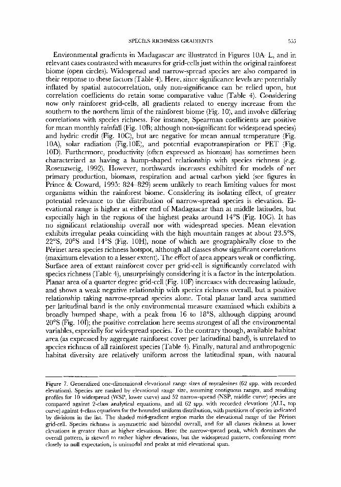
Figure 7. Generalized one-dimensional elevational range sizes of mycalesines (62 spp. with recorded elevations). Species are ranked by elevational range size, assuming contiguous ranges, and resulting profiles for 10 widespread (WSP, lower curve) and 52 narrow-spread (NSP, middle curve) species are compared against 2-class analytical equations, and all 62 spp. with recorded elevations (ALL, top curve) against 4-class equations for the bounded uniform distribution, with partitions of species indicated by divisions in the list. The shaded mid-gradient region marks the elevational range of the Pkrinet grid-cell. Species richness is asymmetric and bimodal overall, and for all classes richness at lower elevations is greater than at higher elevations. Here the narrow-spread peak, which dominates the overall pattern, is skewed to rather higher elevations, but the widespread pattern, conforming more closely to null expectation, is unimodal and peaks at mid elevational span.
556 D. C. LEES ETAL.
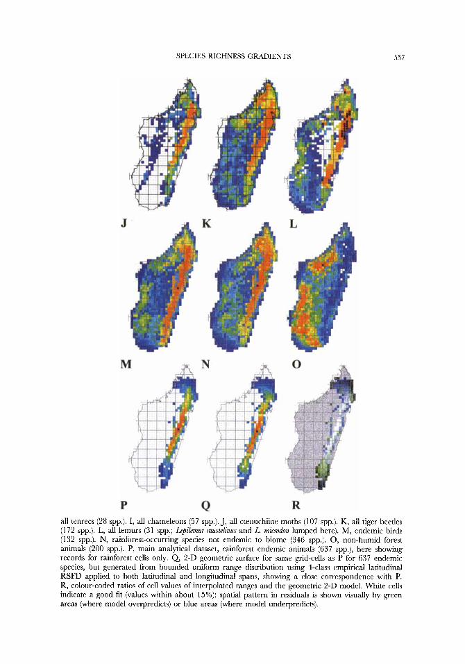
Figure 8. Species richness patterns. WORLDMAP output showing plots of species richness of interpolated ranges (B-P) on a quarter degree grid. An equal frequency scale of colours indicates species richness counts per grid-cell as increasing temperature, with the most depauperate (or for A, most heavily undersampled) cells in blue, the richest cells in red, and the maximal hotspot(s) shown by a black spot. Gaps in interpolated maps are for cells which fall outside all minimum convex polygons. A-M show patterns of species richness for all species in each group; N-P show patterns for habitat classified subsets of species. A (empirical species richness) and B (interpolated species richness) for all taxa (1 183 spp.). C, all enariine beetles (148 spp.). D, mycalesine satyrine butterflies (67 spp.). E, all butterflies excluding mycalesines (255 spp.). F, all frogs (186 spp.). G, all rodents (19 spp.). H,
SPECIES RICHNESS GRADIENTS 557
all tenrecs (28 spp.). I, all chameleons (57 spp.). J, all ctenuchiine moths (107 spp.). K, all tiger beetles (1 72 spp.). L, all lemurs (3 1 spp.; L e p i h u r mustelinus and L. microdon lumped here). M, endemic birds (1 32 spp.). N, rainforest-occurring species not endemic to biome (346 spp.). 0, non-humid forest animals (200 spp.). P, main analytical dataset, rainforest endemic animals (637 spp.), here showing records for rainforest cells only. Q 2-D geometric surface for same grid-cells as P for 637 endemic species, but generated from bounded uniform range distribution using 4-class empirical latitudinal RSFD applied to both latitudinal and longitudinal spans, showing a close correspondence with P. R, colour-coded ratios of cell values of interpolated ranges and the geometric 2-D model. White cells indicate a good fit (values within about 15%); spatial pattern in residuals is shown visually by green areas (where model overpredicts) or blue areas (where model underpredicts).
Figure 9. (A) Ptrinet grid-cell exclusion experiment. Species richness for the original 637 spp. is shown by open circles, and the 632 spp. left after removing all Ptrinet grid-cell records by filled triangles. This sensitivity analysis, although removing 46 species from the Ptrinet grid-cell's fauna, demotes Ptrinet's score to 348 species, just two species below the resulting value of the square two grid-cells to the north. The Ptrinet grid-cell change is arrowed. Clearly, the relative oversampling indicated for this square does not significantly promote the mid-latitudinal parabolic pattern: fourth order polynomials fitted through the points show no shift in central tendency, despite the northwards shift of the hotspot. (B) Longitudinal range exclusion experiment, again for all rainforest endemics (637 spp.). As for 9A, but in this case all longitudinally orientated ranges (45 spp.) are removed. Fourth order polynomials fitted through the points show no significant change in the central tendency or shape of the convex curve, although more species might be expected in the north, due to the greater area and width of the rainforest biome at those latitudes, and thus more longitudinally oriented ranges.
habitat diversity increasing only slightly northwards (Fig. 10K, L), and showing a particularly weak relationship with latitude.
In fact, none of these environmental gradients, for all or just rainforest cells, matches very closely either the general quasi-parabolic shape of the latitudinal species richness curves for taxa examined here, nor the common position of species
SPECIES RICHNESS GIL4DIENTS 559
TABLE 4. Variation explained by environmental and geometric factors, taken independently, for rainforest grid-cells, ranked in order of importance as measured by Spearman's rank correlation coefficient (rho), here including Siegel's correction for shared ranks (first three columns). Pearson's correlation coefficient (?) provides a similar ranking of variables. Widespread (Wsp) and narrow-spread (Nsp) species are compared, but to allow comparison with other factors, no individual adjustments are made here for geometry. Correlation coefficients and significance levels are likely to be inflated by spatial autocorrelation, but, with the exception of elevational range, are greatly reduced by factoring outgeometry(finalco1umn; R=residuals), * =P<O.O5, ** = P < O . O I , ***=P<O.OOl, ns=notsignificant.
Factor ~~ ~
rho rho rho + + All (637 spp.) Wsp (182) Nsp (455) All (637) All (637)
n = 227 n=218 n = 2 2 4 n=223 n=223R
Geometry Land area sum lat. hand Mean elevation Mean annual temperature Potential evapotranspiration Rainforest cover Natural habitat diversity Hydric credit Max elevation Mean monthly rainfall Anthropogenic habitat diversity Area of quarter degree grid-cell Radiation Rainforest cover sum lat. band Elevation range
richness hotspots in Madagascar between 19"s and 17"s. Moreover, correspondence apparent between the species richness profile for narrow-spread species and mean elevation (compare Figs 11D and 10H) is not, in fact, reflected in a higher correlation for narrow-spread species. Of all environmental factors examined here, planar land area comes closest to matching the overall convex one-dimensional pattern of animal species richness, although in marked contrast with the distribution of planar area of rainforest. However, geometry explains more variation than any other factor taken on its own and over twice as much as any factors except land area per latitudinal band (Table 4). Furthermore, land area and rainforest area per latitudinal band are no longer significant in a stepwise multiple regression analysis of this data first factoring out geometry, whereas grid-cell rainforest cover, elevation measures, mean annual temperature, PET and natural habitat diversity retain (or regain in the case of elevational range) explanatory power, each considered individually as potential predictors of residuals among the 637 rainforest endemics (Table 4).
Range orientation sensitiviQ anabsis
Since Madagascar itself is longitudinally widest between 16"s and 19"S, the Ptrinet Effect might nevertheless be promoted by a local surfeit of longitudinally oriented ranges. A further sensitivity analysis was therefore included to assess whether overlap of longitudinally-oriented ranges with latitudinally-oriented ones may be locally augmenting the mid-gradient species richness scores. In fact, removal of all ranges whose longitudinal axis was longer than the latitudinal axis (46 species) has
560 D. C. LEES ETAL.
A y = -0.24~ + 25.75, r2 = 0.12
+.- 1 2 4 : ; I I : ; : : : I : ; : : I 26 25 24 23 22 21 20 19 18 17 16 15 14 13 12 11
Figure 10. Environmental variables for Madagascar. Rainforest biome grid-cells (open circles, n = 336, with fitted regression lines) are contrasted with other gridcells (pluses, n=573) for graphs A-D. A, mean annual temperature modelled logistically on mean elevation per grid-cell derived from 30 arc- second digital elevation model. B, mean monthly rainfall (derived from contours in Ravet, 1952). C, hydric credit expressed as the prec'ipitationlpotential evapotranspiration [PET] ratio (after Ravet, 1952 for rainfall, and formulae and data in Oldeman, 1990). D, mean annual potential evapo- transpiration modelled on temperature and effective radiation (using equations in Oldeman 1990). E, daily solar radiation striking a flat cloudless surface (modelled on latitude after equations in Oldeman, 1990). F, planar area in !an' ofa latitude-longitude grid-cell based on the spherical approximation for the
SPECIES RICHNESS GRADIENTS 56 1
even less effect on the maximum value of a fourth order polynomial fitted through the peak grid-cell values, than for the above PCrinet exclusion experiment, again resulting in no significant difference in central tendency (Fig. 9B; mw = 0.3005, -0.7, with a similar result for the original points: mw=0.3133, -0.7).
Latitudinal species richness gradients of range size classes against null model
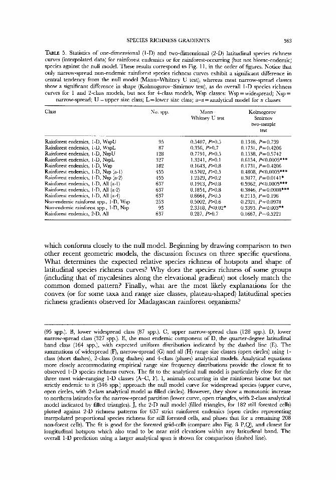
If geometric factors do not play a significant role in dictating gradients of species richness, there should be no obvious relationship for ranked range size classes between range richness patterns and geometric predictions. Graphs for one-dimensional range classifications for rainforest endemics are shown in Figure 1 1A-H, for species occurring in (but not endemic to) rainforest in Figure 111, and the summary for the two-dimensional case in Figure 11J. In fact, for the one-dimensional case, no class shows a significant difference in central tendency from the null model (Table 5) . For widespread species, the species richness profile particularly closely fits that predicted by geometric constraints, and there is no significant difference for the upper narrow-spread class. In contrast, the lower of the narrow-spread classes shows a significantly different profile (Table 5), which is skewed to the north, and this is also reflected in the summed narrow-spread distribution for one and two class models (Table 5). Notice that each doubling of the number of classes in the model increases the fit of the predicted curve to that observed (Kolmogorov-Smirnov test results in Table 5), as the null model effectively integrates more finely the empirical range size frequency distribution. Notice also that for those humid forest species (346 spp.) not exclusive to Madagascar rainforest (Fig. 1 lI), while the curve appears somewhat north-skewed for widespread classes, this difference of fit does not reach significance in the test (Table 5). In contrast, the curve for narrow-spread species, which increases northwards in a monotonic fashion, is significantly different both in central tendency and shape from the null model (Fig. 111; Table 5).
In the case of 2D interpolated ranges for all 637 species, geometry explains most of the variation (Table 4; Fig. 11J). In spite of any mismatch to the empirical longitudinal range size frequency distribution, no significant difference from the 2- D, 4-class null model is found in central tendency, nor in goodness of fit (Table 5) , between peak observed and predicted scores for each latitudinal band. Furthermore, predicted species richness (Fig. 84) is tightly correlated (? = 0.75; Table 4) with interpolated results (Fig. 8P). Correlation is strongest along the spine of the rainforest biome, with residuals concentrated at marginal sites (Fig. 8R).
DISCUSSION
Results presented here demonstrate that latitudinal species richness patterns for a range of rainforest animal groups in Madagascar exhibit a predominant component
respective bounding coordinates: Area = 637 1 -2*(sin(radians(Lat l))-sin(radians(Lat2)))*(radians(Longl)- radians(Long2)). G, elevational range, and H, mean elevation (both based on the 30 arc second digital elevation map, for 498 eastern region grid-cells). I, total planar land area for Madagascar per quarter degree latitudinal band. J, planar rainforest cover per latitudinal band (after map in Green & Sussman, 1990, here calibrated to an estimated total projection of 31,000 km'). K, natural habitat diversity, and L, anthropogenic habitat diversity, both as measured by categories used in interpolation (open triangles, n = 97 1 grid-cells).
Figure 1 1. One-dimensional '1 -D' (A-I) and two-dimensional '2-D' (J proportional species richness (PSR) along the Madagascan latitudinal gradient for 637 strictly endemic rainforest animal species (A-H,J and 346 non-endemic rainforest-occurring species (I). See Table 4 for accompanying statistics. A-D: rainforest species are divided by latitudinal extent into four independent equal-span classes of ranked range size with the one-class null model shown by a dashed line. A, upper widespread class
SPECIES RICHNESS GRADIENTS 563
TABLE 5 . Statistics of one-dimensional (1-D) and two-dimensional (2-D) latitudinal species richness curves (interpolated data) for rainforest endemics or for rainforest-occurring (but not biome-endemic) species against the null model. These results correspond to Fig. 1 1, in the order of figures. Notice that only narrow-spread non-endemic rainforest species richness curves exhibit a significant difference in central tendency from the null model (Mann-Whitney U test), whereas most narrow-spread classes show a significant difference in shape (Kolmogorov-Smirnov test), as do overall 1-D species richness curves for 1 and 2-class models, but not for 4-class models, Wsp classes: Wsp =widespread; Nsp =
narrow-spread; U = upper size class; L = lower size class; a-n = analytical model for n classes
which conforms closely to the null model. Beginning by drawing comparison to two other recent geometric models, the discussion focuses on three specific questions. What determines the expected relative species richness of hotspots and shape of latitudinal species richness curves? Why does the species richness of some groups (including that of mycalesines along the elevational gradient) not closely match the common domed pattern? Finally, what are the most likely explanations for the convex (or for some taxa and range size classes, plateau-shaped) latitudinal species richness gradients observed for Madagascan rainforest organisms?
(95 spp.). B, lower widespread class (87 spp.). C, upper narrow-spread class (128 spp.). D, lower narrow-spread class (327 spp.). E, the most endemic component of D, the quarter-degree latitudinal band class (164 spp.), with expected uniform distribution indicated by the dashed line (E). The summations of widespread (F'), narrow-spread (G) and all (H) range size classes (open circles) using 1- class (short dashes), 2-class (long dashes) and 4-class (pluses) analytical models. Analytical equations more closely accommodating empirical range size frequency distributions provide the closest fit to observed 1-D species richness curves. The fit to the analytical null model is particularly close for the three most wide-ranging 1-D classes (A-C, F'). I, animals occurring in the rainforest biome but not strictly endemic to it (346 spp.) approach the null model curve for widespread species (upper curve, open circles, with 2-class analytical model as filled circles). However, they show a monotonic increase to northern latitudes for the narrow-spread partition (lower curve, open triangles, with 2-class analytical model indicated by filled triangles). J, the 2-D null model (filled triangles, for 182 still forested cells) plotted against 2-D richness patterns for 637 strict rainforest endemics (open circles representing interpolated proportional species richness for still forested cells, and pluses that for a remaining 208 non-forest cells). The fit is good for the forested grid-cells (compare also Fig. 8 P,Q, and closest for longitudinal hotspots which also tend to be near mid elevations within any latitudinal band. The overall 1-D prediction using a larger analytical span is shown for comparison (dashed line).
564 D. C. LEES ETAL.
;The proportional level of the species richness hotspot
Differences in level of proportional species richness of the hotspot can be understood for one-dimensional species richness by considering the interaction of an emergent biological characteristic, the range size frequency distribution (RSFD) of a species array, with the geometric bounding of species ranges. Expected values can be calculated for discrete (e.g. empirically derived) classes using Equation 10. For example, for a uniform probability distribution of range sizes and bounded range placements, peak proportional richness of about 0.693 of the regional pool of species is predicted. For a linearly increasing frequency distribution with decreasing range size, and a uniform distribution of range midpoints within the midpoint constraint envelope, as in Model 2 of Colwell and Hurtt (1994), Equation 10 evaluates the hotspot to 50% of regional richness. This is also the peak value generated by the binomial model of Willig and Lyons (1998). This model generates a true parabola (whose implicit equation, expressed in terms of the present model is r = 2x- 22), where the placement of points defining limits of each range are independently uniformly distributed between two boundaries on the unit line (i.e. in the interval [0,l]). It can be shown that the Willig and Lyons model is precisely equivalent not only to Colwell and Hurtt’s Model 2, but to the second broken stick model of MacArthur (1957) that was applied to niche overlap (Lees and R. K. Colwell, unpublished). In contrast, the model developed here is based on a bounded uniform distribution of ranges for probabilities of x given r (i.e. range limits are distributed uniformly in the interval [0, 1 - r] and [r, 11). Using analytical equations for two classes, widespread and narrow-spread species, provides a simple first order approximation to the empirical range size frequency distribution (Appendix 2). Geometric effects are likely to predominate where the proportion of widespread species is substantial (more than about 0.25); widespread species exert a dis- proportionately large influence (Colwell & Hurtt, 1994; Pineda & Caswell, 1998) above that level, at least at the mid-domain peak.
Although the position of the hotspot is of interest, the shape of the species richness distribution is a more fundamental feature, and differences then become evident in the RSFD of widespread species. For example, a RSFD skew towards more widespread species causes a shift in the species richness distribution away from a convex curve towards a plateau (Fig. 11A). For the interpolated data analysed here, a 4-class, 1 -D analytical approximation is, furthermore, highly predictive of shape. Analytical equations can be readily derived for more accurate predictions using the present approach, but integrating the underlying RSFD itself (which can only be modelled in the case of ‘real’ data) could provide a useful alternative method. Unfortunately, RSFDs seem to be strongly case-dependent. Indeed, the range of patterns exhibited by the taxonomic cross-section examined here cautions against generalizing about range size frequency distributions, as also suggested by Gaston (1998). ‘ Both negatively and positively skewed unimodal distributions are exhibited by some of the ten different focal groups, a strongly bimodal distribution occurs in one group (butterflies), whereas intermediate range size classes tend, for most groups, to be fairly uniform in frequency. Moreover, none of these distributions tend to normality when range sizes are log-transformed, a pattern reported in a number of studies on mammals and birds (e.g. Anderson, 1985; Letcher & Harvey, 1994; Smith, May & Harvey, 1994; Gaston, 1996; Blackburn & Gaston, 1996), although
SPECIES RICHNESS GRADIENTS 565
some do tend to a left log-skew (Gaston, 1998). Patterns thus seem to vary greatly between taxa of differing body-size and mobility, and among the same taxa along different types of environmental gradient. Although in this study the single grid-cell band class appears in some groups to be inordinately large, and intermediate range- size classes seem relatively uniform, the extent to which under-sampling or over- splitting may enhance these tendencies among more localized species is unknown.
The lack of a significant difference of the peak values of the 2-D curve to those predicted by the null model owes largely once again to the curves of more widespread species, which at the hotspots along the more or less perpendicular longitudinal (and essentially elevational) gradient, are still predicted to show a proportional species richness of 1. It is likely that the longitudinal fit would be considerably closer for marginal areas by incorporating the longitudinal range size distribution. For example, the RSFD for mycalesines along the elevational gradient is markedly different. Two problems for modelling species richness gradients thus emerge, also applicable to 1-D analyses. First, should empirical RSFDs be used, for example summarized for each latitudinal band? An alternative and more powerful approach would be to input some generalized RSFD, for example one modelled for a particular group for elevation. Second, how should varying spans be dealt with? For the 2-D surface prediction produced here, the longitudinal span of the habitat (rainforest) was used at each latitudinal band. However, appropriate spans may be dictated by both extrinsic and intrinsic constraints, varying among species in an assemblage (Willig & Lyons, 1998). There thus exists some inevitable compromise in defining the span. The 1-D graph for rainforest non-endemic species (Fig. 11H) may at least in part reflect a more poorly defined northern boundary (the defined span does not include or optimally represent the full range of all species, especially those confined to transitionally humid forest fragments in the north). This case may thus be comparable to Colwell & Hurtt’s (1 994) hybrid model 4, which has one ‘soft’ boundary. Alternatively, perhaps more likely, the graphs may highlight a fundamental difference in distributional patterns between non- endemic and endemic, adaptively radiated species.
This study suggests that accounting accurately both for the RSFD and for appropriate spans are keys to any analysis of species richness. The results also suggest that environmental explanation(s) will be required to account for the general increase of narrowly endemic species richness, and non-endemic species towards the north.
Exceptions
The northwards skew of some groups such as cicindelid beetles and ctenuchiine moths is obvious (Fig. 85, K), and other groups (e.g. chameleons: Fig. 81) show a ‘warmspot’ in the Marojejy region at about 14’s. As seen in Table 1, cicindelids and ctenuchiines, and also chameleons have a particularly low proportion of species known to be widespread, less than the theoretical threshold of about 25% for approximately equal influence. Although this narrow endemism, at least in part, is likely to reflect lack of knowledge, these groups seem the least likely to be strongly influenced by geometric processes. Rather, such taxa seem not to be exceptions at all, but instead seem to exemplify the pattern seen in other groups of northwards increase in species richness for narrow-spread species. However, enariine beetles, which also have a low proportion of widespread species, are richest at middle latitudes, so this is not invariably the case.
566 D. C . LEES E'TAL.
A few smaller groups show either a relatively even or an irregular distribution across the latitudinal gradient, even after interpolation. Plateau-shaped distributions are gen- erally the case for groups of species that tend to have very wide ranges (e.g. birds, Fig. 8M, which are nearly as rich in the north as at middle latitudes), are not endemic to Madagascar, and which may be eurytopic, occurring in other habitats including dry forests. For lemurs (Fig. 8L), there is a polymodal species richness distribution that nowhere exceeds 13-14 species and, unusually, the PCrinet area falls within a trough of 10 predicted species. However, their present day species richness distribution is unlikely to be representative of that in the recent past. Subfossil sites, together with more than 100 years of historical data, chart range contraction for some species (e.g. the genus Hapalemur) within the relatively short timespan of human occupancy of Madagascar, as well as extinction of at least 15 taxa, a third of the total documented fauna (e.g. Jungers et al., 1995). Human influence has been and continues to be par- ticularly severe just east of the capital at 19"s.
An exceptional species richness pattern is also shown by mycalesines for elevation: although the richness hotspot is more or less at the level predicted by the null model and only at slightly higher elevation, the central tendency of the richness distribution is significantly different. Local endemism along the elevational gradient is much higher than for latitude, as expected for a steeper climate gradient (see Janzen, 1967; Huey, 1978) and demonstrated by lapse rates (the mean annual temperature difference in Madagascar is about 10.4"C over 2000 m, but only about 3.1"C over 13 degrees of latitude-values derived from climate data in Oldeman, 1990). The large proportion of narrow-spread species minimizes the potential of geometric effects on the overall pattern, although the unimodal curve exhibited by widespread species suggests some influence here too, of geometric factors. This pattern contrasts sharply with the bimodal pattern exhibited by narrow-spread species, which begs examination within a phylogenetic context (Lees, 1997). The strong asymmetry between species richness at higher and lower elevations is not addressed here, although this is a commonly observed trend globally (Rahbek, 1995). However, occasional freezing temperatures above 2 100 m must severely limit the distribution of many organisms, and this is surely the case for mycalesines. Comparison with elevational richness patterns shown by other taxa is also desirable.
Explanations
A new hypothesis, bounded range overlap, is proposed as an explanation for generally highly parabolic gradients of species richness observed for taxa occurring in the eastern rainforest biome of Madagascar. Three other major hypotheses for species richness gradients (sampling artifacts, area and energy) are also considered.
Bounded range overlap Results strongly suggest that the null model in this study is the most parsimonious
explanation for overall species richness gradients in Madagascar (at least for rainforest endemics). This interaction between geometry and species range distributions is here termed bounded range overlap. For ranked range size partitions within different groups of species, a suite of mutually exclusive classes offers a powerful approach for testing for geometric effects using analytical equations. The main line of evidence
SPECIES RICHNESS GRADIENTS 567
suggesting that bounded range overlap is the factor of over-riding importance in endemic rainforest species richness patterns in Madagascar, is the tight fit to the unusual and symmetric predicted shapes of not just one, but the majority of range size classes. Furthermore, in this study, the position of Madagascar, spanning nearly 14 degrees of latitude entirely in the southern hemisphere, renders possible sharp discrimination between predicted curves due to environmental effects, and predicted effects due to geometry. As suggested by Colwell & Hurtt (1 994) and Willig & Lyons (1 998), biophysical explanations for richness gradients remain inadequate if they do not first control for the effects of geometry imposed by range boundaries. Much greater insight into such potential effects along environmental gradients is likely to be gained, as shown here, not only by comparing with an appropriate null model, but by decomposing species richness patterns into classes of ranked range size, just as is illuminating for species-area curves (Harte & Kinzig, 1997). This way, the relative contributions of ranked range size classes can be clearly analysed.
Failure to reject the null model in most cases in this study raises a new question. Why should quasi-parabolic curves arise from a summation of empirically derived species ranges? Within geometric range midpoint constraints, it is appealing to think that there must be a strong stochastic component in range placement (Lyons & Willig, 1997; Willig & Lyons, 1998), as there may also be, within any large phylogenetic group, in range size. Indeed, the degree of painvise overlap in range placements can be measured against null expectations using the analytical equations of Pielou (1 977), Dale (1 986, 1988) and Sugihara (1 986). Unfortunately, although randomness is measurable, the challenge remains to separate any component of range stochasticity that may be natural against that which is an artifact of sampling effort. It is intuitive that there must be a strong deterministic component influencing range sizes and positions based on extrinsic factors, such as physical barriers and ecotones, and intrinsic factors, such as phylogenetic and ecological constraints in relation to climate and topography (Emlen et al., 1986; Willig & Lyons, 1997). Whether humped species richness curves emerge from largely stochastic or de- terministic processes, however, geometry still imposes constraints on range placements and maximal range sizes, which for summation of large numbers of ecologically diverse species is still likely to generate a domed pattern.
Sampling artgacts Nevertheless, could sampling artifacts still play a major role in generating convex
species richness curves? Efforts have here been made to control for such artifacts, especially in the case of butterflies and for mid-latitudes. However, for tropical datasets especially, sampling artifacts cannot be ruled out any more than taxonomic artifacts (such as over-splitting). This is particularly because the sizes of ranges along latitudinal and elevational gradients (and indeed also, ranges of habitats utilized) are not consistently documented across species. Rather, they will generally be most greatly underestimated for the rarest species and for the areas of highest species richness, even where sample effort is evenly distributed but falls short of exhaustiveness (Colwell & Hurtt, 1994). So if narrow-spread species were also evenly distributed, the hotspot level should here be underestimated at mid latitudes, not overestimated. In fact, because such sampling artifacts are concentrated at the end of the range size frequency spectrum which in general has the least influence on local species richness scores, and considering the ranked range class results, it is highly unlikely
568 D. C . LEES ETAL.
that they can be the cause of the more or less symmetric overall species richness patterns found here.
Habitat area Geographic area, and often more specifically, habitat area, is perhaps the general
factor most frequently linked with geographic variation in species richness (e.g. Rosenzweig, 1995). However, explanations implicating area in fact compound several distinct, possibly interwoven, diversity-generating factors (Gotelli & Graves, 1996), which may operate at different spatial and temporal scales for different taxa. For example, larger areas passively sample more individuals and thus more species (Arrhenius, 1921; Connor & McCoy, 1979), or a more diverse range of habitats (Williams, 1943; Hart & Horwitz, 1991; Scheuring, 1991), sample potential colonists more effectively as an inverse function of distance (MacArthur & Wilson, 1967), are more resilient to extinction (Munroe, 1948; MacArthur & Wilson, 1963; Terborgh, 1973) and have greater allopatric speciation potential (Rosenzweig, 1992, 1995). Such species-area relationships are potentially modified by a variety of taxonomic constraints, such as the fractal relationships of species body size to land surface area (Morse et al. 1988; Sugihara & May, 1990), and by dispersal, which means that regional species pools dominate local richness with little or no evidence for saturation (Caley & Schluter, 1997).
From a mainland biogeographic perspective, although exceedingly difficult to quant- ify, the surface area of a biome available to biodiversity averaged on an evolutionary time-scale may well have influenced richness of the regional species pool. The extent to which analyses can rely on present day planar area and presumed endemic biotic subsets (see e.g. Blackburn & Gaston, 1997) as a proxy is uncertain. At local to meso- scales, theory relating area and separation of habitat fragments with extinction stoch- asticity is provided by metapopulation dynamics (see review by Hanski, 1998). In the case of the Madagascan rainforest biome, habitat fragmentation is probably mostly very recent and anthropogenic in origin, with the largest forest blocks now remaining towards the north. However, the results of human influence in the last two millennia on the latitudinal distribution of local species richness cannot be reliably assessed without good knowledge of subfossil distributions (see Goodman & Patterson, 1997), but a new wave of extinction may already be underway.
Natural fragmentation of montane ecosystems over a time-scale potentially relevant to speciation processes may be of substantial biogeographic significance because of isolation rather than area (Adams, 1977, provides a useful model based on Andean satyrine butterflies). It is now widely recognized that there has been massive potential for range shifting along latitudinal and elevational gradients in response to the Pleistocene climatic oscillations (e.g. Coope, 1994), in Madagascar's case before the arrival of man. At the Last Glacial Maximum for example, the ericaceous transition zone might have been depressed by as much as 800-1000 m. (Burney, 1988, 1996; Straka, 1996), rendering montane isolation for all but the highest mountains temporary. From this Pleistocene vicariance perspective, the large number of peaks above about 1800 m in the north of the rainforest biome may be related to the observed northwards increase in narrow-spread species.
As far as generally decreasing planar area towards higher elevations (e.g. Rahbek, 1997) is concerned, climate change must have caused changes in the elevational distribution of habitat area. Taking account of cyclic opportunities within a bio- geographically connected biome or land area for dispersal to mix the regional pool,
SPECIES RICHNESS GRADIENTS 569
existence of a simple relationship between the density of elevationally restricted species for a given band and habitat area (at any given time) seems implausible. However, if current habitat area along the latitudinal gradient is of any importance due to anthropogenic habitat loss and/or fragmentation, then greater species richness would be expected where habitat area is greatest and least fragmented at about 14-16"s (Fig. lOJ, not at 16-18"s where land area is greatest (Fig. 101). In fact, as shown for most groups here, species richness is greatest at mid-latitude. Even if rainforest until recently stretched continuously as far west as fragments which still occur in the Bongolava massif (Fig. 1; see Gade, 1996, with Burney, 1988 for counter-arguments), and so was formerly more extensive than in the north, the relatively low number of local endemics in this area argues against mid-latitudinal promotion of species origination or maintenance, that might have persisted as a signal through to the present day.
This study has shown that the overall species richness curves are shaped pre- dominantly by more widespread species. So again, this tends to diminish the relevance of classes of explanations related to areal variation within a biome that might at best account for local changes in density of narrow-spread species. Indeed, passive sampling should be irrelevant to species density. In fact, the 8.2% increase in planar area from south to north of Madagascar makes a mid-latitudinal species richness peak all the more surprising, but this effect is likely to be minimal considering the overall slope of an area-biogeographic equation for arbitrary sampling windows of a connected biome, such that species richness will increase much more slowly than area (Preston, 1962; see also Leitner & Rosenzweig, 1997). Furthermore, significant differences are only likely to be manifest in the narrowest ranked range size classes which will display far steeper species area curves, with an exponent exceeding unity (Harte & Kinzig, 1997). For all these reasons, and considering the range orientation test here, it seems highly unlikely that area can account for the peak in latitudinal rainforest species richness curves observed at central latitudes of Madagascar. Whether, and if true mediated by what processes, any of its effects contribute to the more irregular curves shown by narrowly endemic species, species occurring in more fragmented habitats, or for the skewed species richness curve along the elevational gradient exemplified by mycalesine butterflies, remains open to future investigations.
E n w Perhaps the most influential theory proposed in recent years relating environmental
gradients to species richness has been the species-energy hypothesis (Wright, 1983). Furthermore, strong empirical relationships have been reported with measures of atmospheric energy flux, such as annual and potential evapotranspiration, themselves closely correlated with rainfall (e.g. Turner et al., 1987, 1988; Currie, 199 1, and Wylie & Currie, 1993). Such solar energy and moisture gradients were formerly associated with the latitudinal gradient in species richness through the notions of higher favourableness and environmental stability of equatorial tropical rainforest zones (see Pianka, 1966; Terborgh, 1973). Although narrow-spread species also merit further examination in this respect, it is apparent that there is no particularly close latitudinal fit between the overall domed species richness curves observed here and those for environmental variables related directly or indirectly to solar energy, which tend to increase northwards. Taken superficially, the present results might thus be interpreted
570 D. C . LEES ETAL.
as one more example ofthe supposed humped relationship ofdiversity with productivity (e.g. Rosenzweig, 1992, and references therein), but the lack of a precise mechanism for such a relationship renders bounded range overlap more parsimonious and, moreover, geometric theory generates exact predictions which are here shown to be largely satisfied. Although not examined here, a similar argument could be applied to the humped diversity relationship with disturbance, (Connell, 1978). However, considering that the treatment of environmental gradients here has not properly controlled for spatial autocorrelation, and a significant effect of temperature and PET cannot be ruled out even after the effect of geometry has been removed, more thorough statistical testing of the data and models is still called for.
Dispersal and rapid bioclimatic adaptation, which must have occurred during Pleistocene climatic oscillations in Madagascar, would both operate to equilibrate species richness across the generally northwards-increasing environmental gradients. These processes would dilute any excess of origination at the more energetic end of the environmental gradient, in accord with the evolutionary speed hypothesis (Rohde, 1992; see also Rohde, 1997). Therefore, if there has been greater origination at the equatorial end, this should be evident amongst the newest species, which have not yet experienced opportunities for range expansion (as in ‘age and area’: Willis, 1922). The observed northwards departure of narrowly endemic species from null bounded range overlap curves (Fig. 11D) should be cladistically testable, in this respect. By contrast, widespread regional endemics have already by definition expanded their ranges and presumably adapted beyond local environmental optima, and so they no longer appear to reflect any precise set of environmental conditions (localized both in space and time) that may have been more conducive to their origination than any other.
IMPLICATIONS
Results here have far-reaching implications for quantitative biogeography and for indicator group studies, as well as more local implications for conservation efforts in Madagascar.
Implications ~ bounded range overlap for biogeography
Despite the potential for quantitative biogeography apparent from Madagascar’s unique geography and long evolutionary isolation, and thus high levels of endemism, there have been few, if any, macroecological studies on Madagascan biota. Here, a symmetrical, domed, pattern is found within the latitudinal variation in species richness for rainforest biome restricted endemics. This pattern owes largely to widespread species, masking a trend of increasing species richness towards the equator for more narrow-spread species. This analytical result has broad and fundamental biogeographic implications, since latitudinal, elevational and benthic species richness curves have repeatedly been reported to be somewhat hump-shaped or even parabolic (e.g. Rex, 1981; Olson, 1994; Rahbek, 1995 and references therein; Willig & Lyons, 1998; Pineda & Caswell, 1998). Few have dared to suggest that geometry may be the principal common factor underlying these empirical
SPECIES RICHNESS GRADIENTS 57 1
patterns for different gradients (Colwell & Hurtt, 1994; Willig & Lyons, 1998), so the challenge now emerges to re-analyse such data geometrically. The species richness equations described here, which partition species into range size classes and can account for spatial differences in proportional richness, not only make allowance for the extreme paucity of our knowledge of endemics, but also allow more powerful analysis of relationships that may remain, for example, between species richness and area or energy. Furthermore, it must be emphasized that bounded range overlap is not merely an abstract, non-biological concept. Expected levels of sympatric species richness can be estimated given a spatial resolution and set of taxonomic definitions, and within the regional pool, most certainly all species are not equal in their local contribution to species richness. The perspective which emerges here is that species range sizes and positions are dynamic, within extrinsic and intrinsic constraints.
Conservation implications
The results of this study also have significance for future work on biodiversity indicators, and a number of more specific implications for the conservation and bioinventory of Madagascar’s fragde native communities.
7 l e surrogacy issue The concordance between taxa of the species richness hotspot and of species
richness gradients for many of the Madagascan taxa studied here contrasts sharply with the poor overlap found by a number of recent studies at different spatial scales in both temperate and tropical regions (Prendergast et aL., 1993; Lawton et aL., 1998; van Jaarsveld et aL., 1998). A large evolutionary radiation might be anticipated to perform well as an indicator of species richness, in so far as differential adaptation at a range of taxonomic levels may mimic stochasticity in range size and placement (Lees, 1997). However, an appropriate geometric null model incorporating an idealized range size frequency distribution could conceivably be a better predictor overall, than the more or less idiosyncratic distribution of a particular indicator taxon. Key tests need therefore to examine whether indicator taxa perform more efficiently not only than combinations of environmental predictors (ideally, founded on remotely sensed data), but better than geometry combined with some generalized range size frequency distribution, in predicting overall diversity patterns. In fact, bounded range overlap can now be teased out as one fundamental component of spatial autocorrelation within geographic analyses. Thus, it is important to know whether the residual variance from this null model in fact represents additional species richness. The interesting pattern shown by narrowly endemic species is well worth investigating in this respect, as is the degree to which they may reflect geographic patterns in faunal turnover in other taxa.
Consemation priorities Range-restricted species in most groups examined here increase in density towards
the north of Madagascar (see also Raxworthy & Nussbaum, 1995). In terms of local endemism, the northern rainforests may therefore prove to be a higher priority than those at middle and higher latitudes for additional resources for conservation and
572 D. C. LEES E’TAL.
habitat restoration. This local conservation importance is further enhanced by its larger and more viable forested areas, slopes more continuously forested to lower elevations (Green & Sussman, 1990), and mostly still tenuously connected system of reserves. However, northern areas must not be considered in isolation. For all Madagascan protected areas, the current study underlines the vital importance of promoting the protection and restoration of the intervening landscape (which Franklin, 1993, aptly calls the unreserved matrix), now a policy integrated within Madagascar’s National Environmental Action Plan, PE I1 (Ganzhorn et al., 1997), if we are to avert the imminent spectre ofa prison patchwork (Coope, 1994; Cousins, 1994; Sussman, Green & Sussman, 1994; Lees, 1996) of degraded reserves. Promoting habitat connectivity and restoration will help to ensure viability and future faunal enrichment of Ma- dagascar’s biota, by enhancing latitudinal and elevational flexibility for species ranges of all sizes in the face of natural and anthropogenic change. Providing for protection and re-creation oflowland forest areas, against all odds, is an especially critical measure which needs addressing by the country’s conservation policy.
Bioinvento? priorities The excessively sharp and large discontinuity for smallest range size classes within
the range size frequency distributions of many Madagascan animals examined here suggests that ranges of those species may be heavily underestimated and taxa over- split. Bioinventory programmes urgently need to address these problems by expanding and redirecting sample effort to under-surveyed areas (highlighted here most reliably as areas with the largest discrepancy between interpolated and empirical richness of more wide-ranging species). Given the recent focus of sampling for most taxa within reserves (Ganzhorn et al., 1997), the unreserved matrix is a clear bioinventory priority, and urgently needs added incentives for its conservation.
Prospects
It would be intriguing to take a fresh look for geometric patterns within data for other biogeographically self-contained geographic regions or biomes of the world, using appropriately bounded null models and dissections of ranked range size distributions. The Madagascan example suggests that areas with relatively continuous habitat, with ranges polarized along one dimension, and/or spanning shallow environmental gradients, will be the most simple to interpret. Possible examples are the Western Ghats of India, the Andes (Graves, 1988), or coasts and their restricted biota (Pielou, 1977); New Guinea would provide an interesting case where endemic species ranges are potentially parallel with lines of latitude rather than longitude. Continents with a complex mix of biomes or less consistently aligned ranges are likely to prove more challenging to evaluate against null models. To take the example of the Neotropics, which continues to enjoy faunal interchange with areas to the north, and whose species richness patterns tend to be dominated by the vast Amazonian species pool (Patterson et al. 1998), analysing by range size class would be illuminating. However, it is difficult to define non-arbitrarily both the faunal composition and boundaries of subsets considered to have evolved in situ (Blackburn & Gaston, 1997).
Constraints underlying the simple case of one dimensional species richness have
SPECIES RICHNESS GRADIENTS 573
long been ignored by ecologists, but application of more sophisticated null models to empirical data for two or more dimensions (including possibly the time axis, at least in the case of phenologies), promises to yield new insights into quantitative biogeography in marine as well as terrestrial environments (Colwell & Hurtt, 1994). This study does not address local variance in species richness along any given span or gradient (e.g. Currie, 1991), which once sampling anomalies are taken into account, may be explained by other random or deterministic factors. In addition, no consideration is given as to how the effect of bounded range overlap may vary with the spatial resolution of the analysis, a most important area for future studies. A deeper analysis than is possible here of the form of the range size frequency distribution for different groups and gradients remains a challenge. Finally, the relationship of range size frequency distributions to patterns of beta diversity still remains virtually unexplored. Such analyses would begin to tackle the causes of asymmetry in species richness trends across gradients, particularly noticeable in the case of elevation.
Conclusions
This study shows that it will be essential to factor out geometry (using appropriate spans) and to condition by range size, in order to examine other factors that may explain spatial variation in species richness. In fact, bounded range overlap emerges as the best explanation for symmetrically convex species richness gradients in Madagascan animals. However, the general increase of narrowly endemic species richness towards the north suggests that other, presumably environmental or evolu- tionary factors are also significant.
ACKNOWLEDGEMENTS
Funding was provided by BBSRC, Leverhulme Foundation, Xerces Society, Wildlife Conservation Society, USAID, Royal Entomological Society and Linnean Society, Douroucouli Foundation, National Geographic Society, Wildlife Con- servation Society, Center for Conservation Biology, and the Darwin Initiative. Joel Minet, Jacques Pierre and Steve Collins are thanked for access to and/or loans of specimens, while Heritiana Raharitsimba, Jeremy Kuhn and Bernard Turlin kindly made available unpublished butterfly data. Paul Williams helped greatly with creation of the quarter degree grid for Madagascar and allowed use of his program WORLDMAP, whose development was also partly supported by the Darwin Initiative. Environmental Systems Research Institute kindly donated the program Arcview3 and Justin Moat provided some GIS coverages. Dick Vane-Wright, Jim Mallet, Carol Boggs, Clive Moncrieff, George Beccaloni (who also kindly allowed use of his Mann-Whitney program), and Louise Holloway suggested substantial improvements to drafts of this paper. We extend especial thanks to Clive Moncrieff who checked and greatly improved the mathematical section, and to Robert Colwell, whose review encouraged development of the analytical null model. Two anonymous referees also made many helpful comments.
574 D. C. LEES ETAL.
REFERENCES
Abrams PA. 1995. Monotonic or unimodal diversity-productivity gradients: what does competition
Ackery PRY Smith CRY Vane-Wright Rl, eds. 1995. Carcasson$ A j k a n buth j lks : an annotated catalogue
Adams M. 1977. Trapped in a Columbian Sierra. Geographical Magazine 49: 250-254. Agassiz DJL, Nash DRY Godfray HCJ, Lawton JH. 1994. Estimating the spread of small invading
Allen RB, Peet RK, Baker WL. 1991. Gradient analysis of latitudinal variation in Southern Rocky
Anderson S. 1985. The theory of range-size (RS) distributions. American Museum Nouitates 2833: 1-20. Andreone F. 1996. Seasonal variations of the amphibian communities in two rainforests of Madagascar.
Andriamampianina L. 1996. Biogeography of enariine (Melolonthidae) and cicindelid beetles in
Arrhenius 0. 1921. Species and area. Journal ofEcology 9: 95-99. Augustin NH, Mugglestone MA, Buckland ST. 1996. An autologistic model for the spatial
distribution of wildlife. Journal of Applied Ecology 33: 339-347. Austin MP, Nicholls AO, Doherty MD, Meyers JA. 1994. Determining species response functions
to an environmental gradient by means of a p-function. Journal of Pigetation Science 5: 215-228. Bauer AJ, Russell AP. 1989. A systematic review of the genus Umplatus (Reptilia: Gekkonidae), with
comments on its biology. Journal ofNatura1 Histoly 23: 169-203. Bernardi G. 1954. Rtvision des Pierinae de la faune malgache (Lepid. Pieridae). M h o i r e s de L‘lnstitut
Scientijque de Madagascar Sh. E.5: 239-375. Blackburn TM, Gaston KJ. 1996. Spatial patterns in the geographic range sizes of bird species in
the New World. Philosophical Transactions o f the R y a l Socieg B351: 897-912. Blackburn TM, Gaston KJ. 1997. The relationship between geographic area and the latitudinal
gradient in species richness in New World birds. Euolutionaly Ecology 11: 195-204. Blommers-Schlosser RMA, Blanc P. 1991. Amphibiens (premiere partie). Fame de Madagascar
75( 1). Paris: Mustum national #Histoire naturelle. Blommers-Schlosser RMA, Blanc P. 1993. Amphibiens (deuxikme partie). Faune de Madagascar
75(2). Paris: Museum national d’Histoire naturelle. Bohning-Gaese K. 1997. Determinants of avian species richness at different spatial scales. Journal of
Biogeograply 24: 49-60. Burney DA. 1988. Modern pollen spectra from Madagascar. Palaeogeograply, Palaeoclimatology and
Palaeoecology 66: 63-75. Burney D. 1996. Climatic change and fire ecology as factors in the Quaternary biogeography of
theory predict? Ecology 76: 2019-2027.
of the Papilionoidea and Hespemidea o f the Ajbtmfiical Regon. Melbourne: CSIRO.
organisms using information from the public. Global Ecology and Biogeograply Letters 4: 1-8.
In: Lourenqo WR, ed. Bioglographie de Madagascar. Paris: Editions de l’ORSTOM, 397-402.
Madagascar. Unpublished MSc. Thesis, University of Kent at Canterbury.
Madagascar. In: Lourenqo WR, ed. Bioglographie de Madagascar. Paris: Editions de I’ORSTOM, 49-58.
Busby JR. 1991. BIOCLIM - A Bioclimate analysis and prediction system. In: Margules CR, Austin MP, eds. Nature Conservation: cost effective biological surveys and data anabsis. Australia: CSIRO, 64-68.
Cadle JE. 1995. A new species of Boophis (Anura: Rhacophoridae) with unusual skin glands from Madagascar, and a discussion of variation and sexual dimorphism in Boophis albilabrk (Boulenger). <oological Journal ofthe Linnean Sock0 115: 313-345.
Caley MJ, Schluter D. 1997. The relationship between local and regional diversity. Ecology 78:
Carleton MD, Schmidt DF. 1990. Systematic studies of Madagascar’s endemic rodents (Muroidea: Nesomyinae): an annotated gazetteer of collecting localities of known forms. American Muslum Noda tes 2987: 1-36.
Carpenter G, Gillison AN, Winter J. 1993. DOMAIN: a flexible modelling procedure for mapping potential distributions of plants and animals. Biodiuersig and Conservation 2: 667-680.
Colwell RK, Coddington JA. 1994. Estimating terrestrial biodiversity through extrapolation. Philosophical Transactions of the R y a l Socieg B345: 10 1- 1 18.
Colwell RK, H u m GC. 1994. Nonbiological gradients in species richness and a spurious Rapoport Effect. American Naturalist 144: 570-595.
Connell JH. 1978. Diversity in tropical forests and coral reefs. Science 199: 1302-1310.
70-80.
SPECIES RICHNESS GRADIENTS 575
Connor EF, McCoy ED. 1979. The statistics and biology of the species area-relationship. American Naturalist 113: 791-833.
Coope GR. 1994. The response of insect faunas to glacial-interglacial climate fluctuations. Philosophical Transactions of the Royal Socieg B343: 19-26.
Cousins SH. 1994. Taxonomic and functional biotic measurement, or, will the Ark work? In: Forey PL, Humphries CJ, Vane-Wright RI, eds. Systematics and Conservation Evaluation. Oxford: Clarendon Press, 397-419.
Currie DJ. 1991. Energy and large-scale patterns of animal and plant species richness. American Naturalist 137: 27-49.
d’Abrera BL. 1997. Butte2flies of the Ajotmkical re@on, Part 1. Papilionidae, Pieridae, Nymphalidae, Sagridae. 2nd Edition. London: Hill House Publishers.
Dale MRT. 1986. Overlap and spacing of species in a zoned community. Oikos 42: 303-308. Dale MRT. 1988. The spacing and intermingling of species boundaries on an environmental gradient.
Dee TJ. 1986. The endemic birds ofMadagascar. Cambridge: ICBP. Diehl E. 1954. Liste des Ltpidoptkres Rhopalockres rencontres au Sud de Madagascar et surtout sur
le Plateau du Sud. Lz Naturaliste Malgache 6: 61-70. Dixon AFG, Kindlmann P, Leps J, Holman J. 1987. Why there are so few species of aphids,
especially in the tropics. American Naturalist 129: 580-592. E d e n JT, DeJong MJ, Jaeger MJ, Moermond TC, Rusterholz KAY White RP. 1986. Density
trends and range boundary constraints of forest birds along a latitudinal gradient. Auk 103: 791-803. Faramalala MH. 1995. Fornations v&itales et domaine forestier national de Madagascar. Map, scale
1 : 1 .OOO.OOO. New York Conservation International.
Oikos 53: 351-356.
I ,
Franklin JF. 1993. Preserving biodiversity: species, ecosystems or landscapes? Ecological Applications 3: 202-205.
Franklin J. 1995. Predictive vegetation mapping: geographic modelling of biospatial patterns in
Gade DW. 1996. Deforestation and its effects in Highland Madagascar. Mountain Research and Development
GanzhornJU, Rakotosamimanana By Hannah L, Hough J, Iyer L, Olivieri S, Rajaobelina S , Rodstrom C, Tilkin G. 1997. Prioritiesfor biodiversig conservation in Madagascar. Primate Report Special Issue 48-1. German Primate Center.
Gaston KJ. 1996. Species range-size distributions: patterns, mechanisms and implications. Trends in Ecology and Evolution 11: 197-201.
Gaston KJ. 1998. Species range-size distributions: products of speciation, extinction and trans- formation. Philosophical lransactions ofthe Royal Sociep o f Landon B353: 2 19-230.
Gentry AH. 1988. Changes in plant community diversity and floristic composition of environmental and geographical gradients. Annals ofthe Missouri Botanical Garden 75: 1-34.
Glaw F, Vences M. 1994. A Fiel&uia’e to the Amphibians and Reptiles o f Madagascar. Second Edition. Germany: Koln. Privately published.
Gleason HA. 1922. On the relation between species and area. Ecology 3: 158-162. Goodman SM, ed. 1996. A floral and faunal inventory of the eastern slopes of the Reserve Naturelle
Inttgral d’Andringitra, Madagascar: with reference to elevational variation. Fieldiana: 85: 1-3 19. Goodman SM, ed. 1998. A floral and faunal inventory of the eastern slopes of the Reserve Naturelle
Inttgral d’Anjanaharibe-Sud, Madagascar: with reference to elevational variation. Fieldiana 90:
Goodman SM, Andrianarimisa A, Olson LEY Soarimalala V. 1996. Patterns of elevational distribution of birds and small mammals in the humid forests of Montagne D’Ambre, Madagascar. Ecotmpica 2: 87-98.
Goodman SM, Hawkins AFA, Domergue CA. 1997. A new species of vanga (Vangidae, Calzcalicus) from southwestern Madagascar. Bulletin ofthe British Ornithological Club 117: 5-10.
Goodman SM, Langrand 0. 1994. Znuentaire Biologzque Foret de zombitse. Rtcherches pour le Developpement. Strie Sciences biologiques No. Special 1994. Antananarivo: Centre d’Information et de Documentation Scientifique et Technique.
Goodman SM, Langrand 0, Whitney BM. 1996. A new genus and species of passerine from the eastern rain forest of Madagascar. Ibis 138: 153-159.
Goodman SM, Patterson BD, eds. 1997. Natural change and human impact in Madagascar. Washington and London: Smithsonian Institution Press.
relation to environmental gradients. Progress in Physical Geography 1 9 474-499.
16: 101-116.
1-246.
576 D. C. LEES ETAL.
Goodman SM, Pidgeon M, Hawkins AF'A, Schulenberg TS. 1997. The birds of Southeastern Madagascar. Fieldiana 87: 1-1 32.
Goodman SM, Rakotondravony D, Schatz G, WilmL. L. 1998. Species richness of forest-dwelling birds, rodents and insectivores in a planted forest of native trees: a test case from the Ankaratra, Madagascar. Ecotropica 4: 104-1 20.
Gotelli NJ, Graves GR. 1996. Null models in ecology. Washington and London: Smithsonian Institution Press.
Graves GR. 1988. Linearity of geographic range and its possible effect on the population structure of andean birds. Auk 105: 47-52.
Green GM, Sussman RW. 1990. Deforestation history of the eastern rainforests of Madagascar from satellite images. Science 248: 2 12-2 15.
Hall CAS, Standford JA, Hauer FR. 1992. The distribution and abundance of organisms as a consequence of energy balances along multiple environmental gradients. Oikos 65: 377-390.
Hanski I. 1982. Dynamics of regional distribution: the core and satellite hypothesis. Oikos 38: 2 10-22 1. Hanski I. 1998. Metapopulation dynamics. Nature 396: 41-49. Harcourt C, Thornback J. 1990. h u r s ofMadagascar and the Cornoros. The IUCN Red Data Book.
Gland IUCN-The World Conservation Union. Hart DD, Honvitz RJ. 1991. Habitat diversity and the species-area relationship: alternative models
and tests. In: Bell SS, McCoy ED, Mushinsky ER, eds. Habitat structure: the physical arrangements o f objects in space London: Chapman & Hall, 47-68.
Harte J, Kinzig, AP. 1997. On the implications of species-area relationships for endemism, spatial turnover, and food-web patterns. Oikos 8 0 417427.
Holloway JD. 1987. Macrolepidoptera diversity in the Indo-Australian tropics: geographic, biotopic and taxonomic variations. Biological Journal of the Linnean Sociep 30: 325-34 1.
Huey RB. 1978. Latitudinal pattern of between-altitude faunal similarity: mountains might be 'higher' in the tropics. American Naturalist 12: 225-229.
Janzen DH. 1967. Why mountain passes are higher in the tropics. American Naturalist 101: 23349. Janzen DH. 1981. The peak in North American ichneumonid species richness lies between 38' and
Janzen DH, Atamff My Farinas M, Reyes S, Rincon N, Soler A, Soriano P, Vera M. 1976. Changes in the arthropod community along an elevational transect in the Venezuelan Andes. Biotropica 8: 193-203.
42"N. Ecology 62: 532-537.
Jenkins M, ed. 1990. Madagascar: pmj l de l'enuironnement. Gland, Switzerland IUCN. Jungers WL, Godfi-ey LR, Simons EL, Chatrath, PS. 1995. Subfossil Zndri indri from the Ankarana
Kerr JT, Packer L. 1997. Habitat heterogeneity as a determinant of species richness in high-energy
Kouki J, Niemela P, Viitasaari M. 1994. Reversed latitudinal gradient in species richness of sawflies
Kremen C. 1992. Assessing the indicator properties of species assemblages for natural areas monitoring.
Kremen C. 1994. Biological inventory using target taxa: a case study of the butterflies of Madagascar.
Langrand 0. 1990. Guide to the Birds ofMadapascar. London: Yale University Press. Lawton JH, MacGarvin M, Heads PA. 1987. Effects of altitude on the abundance and species
richness of insect herbivores on bracken. Journal ofAnima1 Ecalog~ 56: 147-160. Lawton JH, Bignell DE, Bolton B, Bloemers GF, Eggleton P, Hammond PM, Hodda M,
Holt RD, Larsen TB, Mawdsley NA, Stork NE, Srivastava DS, Watt AD. 1998. Biodiversity inventories, indicator taxa and effects of habitat modification in tropical forest. Nature 391: 72-75.
Lees DC. 1996. The Pkrinet Effect? Diversity gradients in an adaptive radiation of butterflies in Madagascar (Satyrinae: Mycalesina) compared with other rainforest taxa. In: Lourenqo WR, ed. Biogkopaphie de Madagascar Paris: Editions de YORSTOM, 479-490.
Lees DC. 1997. Systematics and biogeography of Madagascan mycalesine butterflies (Lepidoptera: Satyrinae). Unpublished D.Phil. Thesis, London University.
Leitner WA, Rosenzweig ML. 1997. Nested species-area curves and stochastic sampling: a new theory. Oikos 79: 503-512.
Lennon JJ, Turner JRG, Connell D. 1997. A metapopulation model of species boundaries. Oikos
Massif of northern Madagascar. American Journal of Physical Anthropology 97: 357-366.
Letcher AJ, Harvey PH. 1994. Variation in geographical range size among mammals of the
Linder HP. 1991. Environmental correlates of patterns of species richness in the south-western Cape
Lyons SKY Willig MR. 1997. Latitudinal patterns of range size: methodological concerns and
MacArthur RH. 1957. On the relative abundance of bird species. Proceedings ofthe National Acadmy of
MacArthur R, Wilson EO. 1963. An equilibrium theory of island biogeography. Evolution 17:
MacArthur R, Wilson EO. 1967. The theov of island biogeography. Princeton: Princeton University
McGuinness KA. 1984. Equations and explanations in the study of species-area curves. Biolo&al
MacPhee RDE. 1987. The shrew tenrecs of Madagascar: systematic revision and holocene distribution
McCoy ED. 1990. The distribution of insects along elevational gradients. Oikos 58 312-322. Mittermeier RAY Konstant WR, Nicholl ME, Langrand 0.1992. h u r s ofMadagascar: An Action
Planfor their Conservation 1993-1999. Gland IUCN. Mittermeier RA, Tattersall I, Konstant WR, Meyers DM, Mast RB. 1994. h u r s OfMadagascar.
Washington: Conservation International. Morse DRY Stork NE, Lawton JH. 1988. Species number, species abundance and body length
relationships of arboreal beetles in Bornean lowland rain forest trees. Ecological Entomology 13: 25-37. Munroe EG. 1948. The geographical distribution of butterflies in the West Indies. Unpublished D.
Phil. Thesis, Cornell University. Nelson R, Homing N. 1993. Forednon-forest classification of Madagascar from AVHRR data:
AVHRR-LAC estimates of forest area in Madagascar, 1990. International Journal $Remote Sm‘ng
Nicoll M, Langrand 0. 1989. Madagascar: Revue de la Conservation et Aires Aotdgies. Gland, Switzerland
Nicholls AO. 1989. How to make biological surveys go further with generalised linear models.
Nix HA. 1986. A biogeographic analysis of Australia elapid snakes. In: Langmore R, ed. Australian
Oberthtir C. 1923. [Entomologising in Madagascar]. Etudes de fi~ziio~temlogiz Comkarie 21 [plates]. O’Brien EM. 1993. Climatic gradients in woody plant species richness: towards an explanation based
O’Brien EM. 1998. Water-energy dynamics, climate, and prediction of woody plant species richness:
Oldeman LR. 1990. An agroclimatic characterisation of Madagascar. ISRIC Technical Paper 2 1.
Olson DM. 1994. The distribution of leaf-litter invertebrates along a Neotropical altitudinal gradient.
Owen JG. 1989. Patterns of herpetofaunal species richness: relation to temperature, precipitation and
Palmer MW, White PS. 1994. Scale dependence and the species-area relationship. Amerian Naturalist
Patterson BD, Stotz DF, Solari S, Fitzpatrick JW. 1998. Contrasting patterns of elevational zonation for birds and mammals in the Andes of southeastern Peru. Journal of Biogeography 25:
Paulian R, Bernardi G. 1951. Les Eurema de la rkgion Malgache (Lep. Pieridae). Naturalist Makache
Paulian R, Viette P. 1968. Insectes LCpidoptkres Papilionidae. Faune de Madagascar 27. Antananarivo/
Pianka ER. 1966. Latitudinal gradients in species diversity: a review of concepts. American Naturalkt
Pielou EC. 1977. The latitudinal spans of seaweed species and their patterns of overlap. Journal of
Palearctic. Am&an Naturalist 144: 30-42.
Province of South Africa. Journal of Biogeography 18 509-5 18.
empirical evaluations for New World bats and marsupials. Oikos 79: 568-580.
Sciences USA 43: 293-295.
373-387.
Press.
Reviews: 59: 423-440.
of Micmgale (Tenrecidae, Insectivora). American Museum Jvovitates 2889: 1-45.
14: 1463-1475.
WWF.
Biological Conservation 50 5 1-75.
Flora and Fauna Series No. 7. Canberra: Australian Goyernment Publishing Service, 4-15.
on an analysis of southern Africa’s woody flora. Journal ofBiogeography 20: 181-198.
an interim general model. Journal DfBiogeography 25: 379-398.
Wageningen: International Soil Reference and Information Centre.
Journal of Tmpical Ecology 10: 129-150.
variance in elevation. J o u m l OfBiogeograph 16: 141-150.
144 717-740.
593-607.
3 139-154.
Paris: ORSTOM/CNRS.
100: 36-40.
Biogeography 4 299-3 1 1.
578 D. C. LEES ETAL.
Pierre J. 1994. Les Acraeidae des Comores et de Madagascar (Lepidopttres Rhopaloctres). Entomolopzste
Pineda J. 1993. Boundary effects on the vertical ranges of deep-sea benthic species. Deep Sea Research
Pineda F, Caswell H. 1998. Bathymetric species-diversity patterns and boundary constraints on
Preston FW. 1960. Time and space and the variation of species. Ecology 41: 61 1-627. Preston FW. 1962. The canonical distribution of commonness and rarity: Part I. Ecology 43: 185-215. Prince SD, Coward SN. 1995. Global primary production: a remote sensing approach. Journal of
Rahbek C. 1995. The elevational gradient of species richness: a uniform pattern?. Ecography 1 8
Rahbek C. 1997. The relationship among area, elevation and regional species richness in Neotropical birds. American Naturalist 149: 875-902.
Rakotoarison N, Zimmermann H, Zimmermann E. 1997. First discovery of the hairy-eared dwarf lemur (Allocebus trichotis) in a highland rain forest of Eastern Madagascar. Folia Primatologica
48: 351-364.
(1) Oceanographic Research Papers 40: 2 179-2 192.
vertical range distributions. Deep-sea Research (ZJ %pica1 Studies in Oceanography: 45: 83- 10 1.
the coincidence of diversity hotspots and conservation strategies. Nature 365: 335-337.
Biogeografity 22: 815-835.
200-205.
68 86-94. Rapoport E. 1982. Areograpty, geographical strategies o f species. Oxford Pergamon Press. Ravet J. 1952. Notice sur la climatologie de Madagascar et des Comores. Mhoires de I'Znstitut Sczentjfique
de Madagascar (D) 4: 1-36. Raxworthy CJ, Nussbaum RA. 1994. A rainforest survey of amphibians, reptiles and small mammals
at Montagne d'Ambre, Madagascar. Biological Conservation 69: 65-73. Raxworthy CJ, Nussbaum RA. 1995. Systematics, speciation and biogeography of the dwarf
chameleons (Brookesia; Reptilia, Squamata, Chamaeleonidae) of northern Madagascar. Journal of
Raxworthy CJ, Nussbaum RA. 1996. Montane amphibian and reptile communities in Madagascar.
Reed KEY Fleagle JG. 1995. Geographic and climatic control of primate diversity. Pmceedirgs ofthe
Rex MA. 1981. Community structure in the deep sea benthos. Annual Review ofEcology and Systematics
Rohde K. 1992. Latitudinal gradients in species diversity: the search for the primary cause. Oikos 65:
Rohde K. 1997. The larger area of the tropics does not explain the latitudinal gradient in species
Rosenzweig ML. 1992. Species diversity gradients: we know more and less than we thought. Journal
Rosenzweig ML. 1995. Species diversib in space and time. Cambridge: Cambridge University Press. Ruggiero A, Lawton JH. 1998. Are there latitudinal and altitudinal Rapoport effects in the geographic
Safford R, Duckworth W. 1988. A M.zldlij2 survg o f M a y ' & Nature Reserve. Cambridge: ICBP. Scheuring I. 1991. The fractal nature of vegetation and the species-area relation. 'Theoretical Population
Schmid J, Kappeler PM. 1994. Sympatric mouse lemurs (Microcebus spp.) in Western Madagascar.
Schmida A, Wilson MV. 1985. Biological determinants of species diversity. Journal of Biogeography
Smith FDM, May RM, Harvey PH. 1994. Geographic ranges of Australian mammals. Journal of
Sokal RR, Rohlf FJ. 1981. Biometry: theprinciples andpractice of stahtics in biological research. San Francisco:
Stempffer H. 1954. Etude sur la RCpartition GCographique des Lycaenidae de Madagascar. Mhoires
Stevens GC. 1989. The latitudinal gradient in geographical range: how so many species coexist in
Stevens GC. 1992. The elevational gradient in altitudinal range: an extension of Rapoport's latitudinal
<0010gy 235: 525-558.
Conservation Biology 10: 750-756.
National Academy of Sciences ofthe United States ofAmerica 92: 7874-7876.
de l'lnstitut Scientjfique de Madagascar E5: 2 19-237.
the tropics. Amerikan Naturalist 133: 240-256.
rule to altitude. American Naturalist 140: 893-91 1.
SPECIES RICHNESS GRADIENTS 579
Straka H. 1996. Histoire de la vtgttation de Madagascar Oriental dans les derniers 100 millenaires.
Sugihara G. 1986. Shuffled sticks: on calculating nonrandom niche overlaps. American Naturalist 127: In: LourenGo WR, ed. Biogiographie de Madagascar. Paris: Editions de I’ORSTOM.
554-560. Sugihara G, May RM. 1990. Application of fractals in ecology. Trends in Ecolosy and Evolution 5:
79-86. Sussman RW, Green GM, Sussman LK. 1994. Satellite imagery, human ecology, anthropology,
Tattersall I. 1982. 7 h e Primates ofMadagaxar. New York: Columbia University Press. Terborgh J. 1971. Distribution on environmental gradients: theory and a preliminary interpretation
of distributional patterns in the avifauna of the Cordillera Vilcabamba, Peru. Ecology 52: 23-40. Terborgh J. 1973, On the notion of favourableness in plant ecology. American Naturalist 107: 481-501. Terborgh J. 1977. Bird species diversity on an Andean elevational gradient. Ecolosy 58: 1007-1019. Thompson PM, Evans MI, eds. 1991. A sum9 ofAmbatovaky Special Reserve, Madagascar. London:
Madagascar Environmental Research Group. Tilman D, Pacala S. 1993. The maintenance of species richness in plant communities. In: Ricklefs
RE, Schluter D, eds. Species diversaty in ecological communities. Chicago: University of Chicago Press,
Turner JRG, Gatehouse CM, Corey CA. 1987. Does solar energy control organic diversity? Butterflies, moths and the British climate. Oikos 48: 195-205.
Turner JRG, LennonJJ, GreenwoodJJD. 1996. Does climate cause the global biodiversity gradient? In: Hochberg ME, Clobert J, Barbault R. Aspects of the Genesis and Maintenance 0s Biological Diversity. Oxford: Oxford University Press, 119-2 10.
Turner JRG, Lennon JJ, Lawrenson JA. 1988. British bird distributions and the energy theory. Nature 335 539-541.
US Board of Names. 1955. Madagascar, Rhnion and the Comom Islands. Ofiial standard names approved the United States Board on Geographic Names. Washington: Office of Geography, Dept. of the Interior, USA.
Vences My Glaw F, Andreone F. 1997. Description of two new frogs of the genus Mantidactylus from Madagascar, with notes on Mantidactylus klemma’ (Guibt, 1974) and Mantidactylus webbi (Grandison, 1953) (Amphibia, Ranidae, Mantellinae). Agtes 14: 130-146.
and deforestation in Madagascar. Human Ecolosy 22: 333-354.
13-25.
Viette P. 1956. Insectes Ltpidoptkres Hesperiidae. Faune de Madagascar, 3. Viette P. 1972. Contribution A I’ttude des satyrides du massif de I’Andringitra, Madagascar-Centre
Viette P. 1991. Chief field stations where insects were collected in Madagascar. Faune de Madagascar
Wallace AR. 1878. Tmtical nature and other essgys. London: Macmillan. Williams CB. 1943. Area and the number of species. Nature 152: 264-267. Williams PH. 1998. WORLDMAP iv WINDOWS: Software and help document 4.1. Privately
distributed by the author, London. Williams PH, Prance GT, Humphries CJ, Edwards KS. 1996. Promise and problems in applying
quantitative complementary areas for representing the diversity of some Neotropical plants (families Dichapetalaceae, Lecythidaceae, Caryocaraceae, Chrysobalanaceae and Proteaceae). Biological Journal of the Linnean Society 5 0 125-157.
Willig MR, Lyons SK. 1998. An analytical model of latitudinal gradients of species richness with an empirical test for marsupials and bats in the New World. Oikos 81: 93-98.
Willis JC. 1922. Age and area: a s t u 4 in geographical distribution and o e n in species. Cambridge: Cambridge University Press.
Wolds H. 1987. Altitude, habitat and tropical insect diversity. Biolop.ical3oumal of the Linnean Society
Wright DH. 1983. Species-energy theory: an extension of species-area theory. Oikos 41: 496-506. Wylie JL, Currie DJ. 1993. Species-energy theory and patterns of species richness: I. Patterns of
bird, angiosperm, and mammal species richness on islands. Biological Conservation 63: 137-144.
pep . Nymphalidae Satyrinae]. Bulletin de la Sociitk Entomologique de France 76: 146-154.
Suppl. 2. Privately published by the author.
30: 313-323.
580 D. C. LEES ETAL.
APPENDIX 1
Habitat &es used in interpolation Code Habitat description
J K L M N 0 P Q R
~~
Moist forest, transitional between rainforest and deciduous (6. 1500 mm p.a.) Baobabs Humid and subhumid littoral (sandy coastal) forest Moist to dry deciduous forest (c. 500-1 500 mm p.a.) Roads (major/minorj Mud-flats Moist gallery/riparian forest Montane ericaceous forest (Philippiu) Sisal plantations Floodplains, inundated areas Lakes Moist limestone (karstic) forest (deciduous-subhumid) Marsh Towns Rice paddies Plantations (Eucu&~ptus, pine, coffee etc.) Sugar cane plantations Perhumid, humid and subhumid rainforest (> I500 mm p.a.) Savannah grasslands (degraded, Arirtzdu-dominated) Subarid thorn scrub (Didiereaceae) (300-500 mm p.a.) Tapia (Uupaca 6ojm) forest Mangrove Secondary formation (‘savoka’j Sandy beaches, riversides, dunes. Wooded savannah or shrubby scrub
APPENDIX 2
Interpolation algorithm
The algorithmic procedure for interpolation is described below: (1) Database habitat preferences (according to Appendix 1) and maximum and minimum elevation
for each species, having databased corresponding parameters for each grid-cell. (2) Produce filtered list of all grid-cells with habitat (above a given threshold area) of type that
accords to species habitat preferences, and with elevation range overlapping the recorded elevational range (even if a single value). The following MS Excel formula generates an interpolated list, where cell reference A1 . . . n gives grid-cell minimum elevation, B2 . . . n gives grid-cell maximum elevation, and C2 . . . n gives a single grid-cell habitat code; corresponding species parameters are in Dl-D3. This formula will automatically generate the predicted list of interpolated cells by returning 1 for predicted presence. Additional habitat parameters can be accommodated as comma-delimited ar- guments within the parentheses after the OR command.
= IF((D$l<=$Bl)*AND(D$2> =$Al)*OR(D$3=$Cl),l,””)
The list can then be imported as an integer comma-delimited text file for import into WORLDMAP, recoded as different confidence levels as necesary, and grid-cells falling outside the MCP disqualified as shown in Figure 2.
(3) Add empirical records to the extrapolative map (scored as confidence level l), as confidence level 2 (reliable records) or 3 (unreliable records). (4) Draw a minimum convex polygon by rotating a line around the vertex of each outlying level 2
grid-cell until the line touches another grid-cell, around which the process is continued until a minimum convex polygon is drawn which encloses all reliable records. This is extremely simple to construct by hand. An appropriate script for generating the MCP (convex hull) around a point distribution using Arcview 3 is available on the ESFU ArcScripts web site.
(5) Delete all confidence level 1 grid-cells whose centroid falls outside the perimeter of this polygon.
SPECIES RICHNESS GRADIENTS 581
APPENDIX 3
Mathematical details of null model
Consider an array of species occurrences of range size r, where r is distributed over the interval [0, 11, representing a one-dimensional geographic span or domain X. Assume that these species ranges are constrained to occur between two hard boundaries at x = O and x = 1, that they have a uniform frequency distribution of spans, and that the lefthand (lower) range boundary of r is distributed with a uniform probability of occurrence over the interval [0, 1 -r]. Assume also that each species span is unfragmented so that Pr(occurrence) = 1 between its range limits. Considering the indeterminancy of the location of the species span, its probability of occurrence at a point x along X is referred to as prl,. The average value of this probability density for any position of x we call PSR (proportional species richness), which may then be multiplied by the total number of species in the array, to obtain the predicted number of species.
For convenience, we select the left range boundary to represent the freedom of location of the species span in relation to the domain and to x. For a species having a range span r, wholly contained within the [0, 11 interval, the left boundary is constrained to lie in [0, 1 - r ] . For this range to be intersected by a value of x , the left boundary must exceed x-r and cannot exceed x. It follows, therefore, that the possible left boundary values of a species span which can give rise to an intersection at x are constrained to lie in the interval
[ M A X ( O , x - r ) , MIN(1 -T ,x ) ] .
There are four domains which geometrically correspond to the different possible combinations of these values (see Fig. 12). This results in the equations describing point probabilities of overlap of x given r for the triangular domains A,B,C, and C’, which are shown in the two-way Table 6 below, and in Figure 3A, 12.
Probabilities of occurrence can be obtained by subtracting the appropriate smallest value from the appropriate largest value, and dividing by the span [ 1 - r] over which any left hand range boundary (and so any species span) is free to occur. Thus we have:
(Eqn 1) MLN(1 - q x ) - M 4 X ( x - q 0 )
1 - r PLI =
Due to the bilateral symmetry along X, the resulting proportions for x 2 0.5 can be reflected around x = 0 . 5 (interchanging x and 1 - x ) . Considering, now just the case x 1 0 . 5 , and taking Equations 1A-C
1
x = r
r
x = 1-r
0 X 1
Figure 12. Domains for null model within unit square, where x represents position on a one-dimensional domain, and r represents increasing ranked range size (see Fig. 3A for more details).
582 D. C. LEES ETAL.
TABLE 6. Derivation of pxl, for null model domains. A, B, C, and C’ correspond to the geometric divisions in Fig. 3A, with column and row titles indicating the appropriate domains. Probability density, pr l , , derived for each of these domains is represented by Equations 1A-C (region C’ being the reflection of C around x=O.5, for which x and 1 - x are transposed), These equations are the basis of the
analytical null model
px,, = [Domain: Fig. 3A] x>(l -r) x<(l -r)
(1 -3-0 [A] ~- - 1 (1 - r )
(Equation 1A)
(Equation 1C’)
x-0 x
( 1 -r) (1-r) [C:]-=-
(Equation 1C)
x - ( x - r ) r ([B:] y)=- (1 - (1-r)
(Equation IB)
from Table 6, we can now derive an analytical result for proportional species richness for all species in an array:
= -ln(l -x)-x)+xln(l-x)-ln(x)+x
=in( k) + xln( 9) = -(1 -x)ln(l -x)-xln(x)
Since real species ranges may contain gaps, equation 2 describes bounds on one dimensional species richness for an entirely uniform range size frequency distribution. Furthermore, since empirical range size frequency distributions may be non-uniform, we may want to approximate them by deriving equations for partitions of the data. An alternative approach is to integrate under an empirical range size distribution r=Jx), but it is not yet known what function, if any, is typical for a given group. The first order approximation is to divide the overall ranked species pool into two portions. The equation for the contribution to proportional species richness (PSR’) of widespread species (where r > 0.5, x < 0.5) is thus:
= x( - In(x) + ln(0.5)) + x
SPECIES RICHNESS GRADIENTS 583
= x l n ( y ) + x
Similarly, for narrow-spread species (where rlO.5, x l 0.5):
= -ln(l-r)-r + -ln(l-r) [ I: d 1: = - h ( l -~)-x+x(-ln(0.5))+ln(l-x)
= In( +-) + xln( z) - x
As used in this paper, analytical equations for a second order bisection of range size frequency classes for x10.5 may be derived just as for Equation 2 by integrating Equations IA, 1B and 1C between the limits indicated in Figure 3A for the respective domains A,B,C. Geometry dictates that four quartiles of ranked range size must be represented by a minimum of 8 different equations, one for each square in Fig. 3B; counterparts for x 2 0 . 5 may be obtained by transposing all x and (1 -x). As a simple check, the above equations for r10 .5 and r20.5 can be derived additively from either left hand column of Fig. 3B, since different equations balance out; however, for each quartile, separate equations for P,,, must be applied for O l x 1 0 . 2 5 and 0 . 2 5 I x l 0 . 5 .
We are now ready to consider in more detail the case where the ranked range size distribution is non-linear (the range-size frequency distribution is non-uniform). Approximation to empirical dis- tributions may be obtained by summing the contributions for each range size class, which may contain different numbers of species. Now, the relationship between an integral of a probability density function p,,? and its average, evaluated between two values of r, may be expressed as follows:
-
Px,dr=h;itx) = (rmax -rrnm)Px,r
where &) is a function of x describing the contribution to proportional species richness (PSR’) of class i (e.g. applicable formulae taken from Fig. 3B). Therefore,
Also by simple proportions, for a non-uniform range size frequency distribution
PSR = Pc:&& + P C ~ G + . . . Pcn= (Eqn 6)
where C, , are mutually exclusive range size classes and P is the proportion of species in any class. Thus, we can estimate the expected proportional species richness by substitution of the right side of Equation 5 into Equation 6. Therefore (in the case of >2 classes),
A simple special case of this proportionality is the case of peak ((‘hotspot”) species richness along a gradient, where x=O.5, here for a 2-class approximation for the uniform distribution. Let P, be the proportion of widespread species (where r20.5), and now let P_=Y. For x=O.5 , it follows from Equations lA, 1B and 7 that
584 D. C. LEES ETAL.
0.5
1-Y 0.5
= ---+ - ln(0.5) - 0.5) + Y
= Y + ( 1 - Y)(21n(2) - 1)
For example, where Y =0.5, PSRr0.5 + 0.5(0.3863)20.6931, But where Y =0.75, PSRg0.75 + 0.25(0.3863)~0.8466 It follows from Equation 8 that a 2-class approximation for overall 1-D species richness at the
hotspot is given by
where S,, denotes the total number of species at the peak (= “hotspot”) and S denotes the total number of species in the array (=“regional species pool”). Expressing this another way,
S,, x S(Y + (( 1 - Y)(21n(2) - 1))) (Eqn 9)
Sm,xS,+(21n(2)- 1)SNxS,+0.3863 SN (Eqn 9 4 where S, denotes the total of widespread species, SN the total of narrow-spread species, and the narrow-spread coefficient is that for the uniform distribution.
The coefficient for any narrow-spread partition of ranked range size kNs is derived from the average probability density of r/(l - r ) evaluated between upper limit a and lower limit b. Following from Equation 5 we have:
- -ln(l-a)+ln(l -b ) -a+b - a - b
The analytical results above and in Figure 3B have been used here to generate expected species richness curves for different ranked range partitions.