Page 1
A numerical model for ocean ultra-low frequency noise:Wave-generated acoustic-gravity and Rayleigh modes
Fabrice Ardhuin, Thibaut Lavanant, and Mathias ObrebskiIfremer, Laboratoire d’Oc�eanographie Spatiale, Plouzan�e, France
Louis Mari�eIfremer, Laboratoire de Physique des Oc�eans, UMR6523 CNRS/Ifremer/IRD/UBO Plouzan�e, France
Jean-Yves Royer and Jean-Francois d’EuDomaines Oc�eaniques, CNRS, Plouzan�e, France
Bruce M. Howe and Roger LukasSchool of Ocean and Earth Science and Technology, University of Hawaii at Manoa, Honolulu, Hawaii
Jerome AucanLaboratoire d’Etudes en G�eophysique et Oc�eanographie Spatiale, Toulouse, France
(Received 9 July 2012; revised 8 April 2013; accepted 9 April 2013)
The generation of ultra-low frequency acoustic noise (0.1 to 1 Hz) by the nonlinear interaction of
ocean surface gravity waves is well established. More controversial are the quantitative theories
that attempt to predict the recorded noise levels and their variability. Here a single theoretical
framework is used to predict the noise level associated with propagating pseudo-Rayleigh modes
and evanescent acoustic-gravity modes. The latter are dominant only within 200 m from the sea
surface, in shallow or deep water. At depths larger than 500 m, the comparison of a numerical noise
model with hydrophone records from two open-ocean sites near Hawaii and the Kerguelen islands
reveal: (a) Deep ocean acoustic noise at frequencies 0.1 to 1 Hz is consistent with the Rayleigh
wave theory, in which the presence of the ocean bottom amplifies the noise by 10 to 20 dB; (b) in
agreement with previous results, the local maxima in the noise spectrum support the theoretical
prediction for the vertical structure of acoustic modes; and (c) noise level and variability are well
predicted for frequencies up to 0.4 Hz. Above 0.6 Hz, the model results are less accurate, probably
due to the poor estimation of the directional properties of wind-waves with frequencies higher than
0.3 Hz. VC 2013 Acoustical Society of America. [http://dx.doi.org/10.1121/1.4818840]
PACS number(s): 43.30.Nb, 43.30.Ma, 43.30.Pc [JAC] Pages: 3242–3259
I. INTRODUCTION
Ultra-low frequency acoustic noise (ULF, 0.1 to 1 Hz)
has been observed from shallow water1 to all depths of the
deep ocean.2,3 At large depths, noise has been associated
with seismic pseudo-Rayleigh waves that propagate over
thousands of kilometers,3,4 from oceans to land. The term
“pseudo-Rayleigh” is also used for the same modes gener-
ated by earthquakes, and it emphasizes the effect of the
water layer in which the motion is a superposition of
obliquely propagating sound waves.5 In the crust, the ampli-
tude of motion decays with depths, similar to usual Rayleigh
waves, with a combination of shear and compression waves
that gives zero tangential stress on the ocean bottom. For
simplicity we will omit the “pseudo” and, even in the
oceans, we will use the term “Rayleigh” waves. These waves
propagate slower than the shear wave speed in the crust and
usually faster than the speed of sound in water.6 These are
clearly seismo-acoustic waves that propagate from oceans to
land, where they produce typical vertical ground surface dis-
placements (VGSDs) on the order of a few micrometers,
which generally dominate seismic records. That propagation
is not yet fully understood and the horizontal gradients in
crust properties and water depth may be responsible for
strong reflection and scattering.
Close to the ocean surface, ULF noise is consistent with
forced gravity waves,2 which are also influenced by the com-
pressibility of water, and that we will call acoustic-gravity
(A-G) modes. Both types, Rayleigh (R) and A-G motions are
forced by near-surface nonlinear hydrodynamic interactions
of ocean surface gravity waves (OSGWs).5,7,8
The objective of the present paper is to verify this theory
quantitatively using pressure records from oceanic locations.
This effort is a logical extension of the validation of seismic
noise models at land locations.9,10 Although land-based seis-
mometers have been very useful to verify the modeled pat-
terns of noise sources in space and time,11 the noise models
still suffer from inaccurate seismic attenuation and propaga-
tion, so that model-data mismatches are difficult to interpret.
The interpretation of acoustic noise in the ocean is more
direct, because it avoids the propagation from ocean to conti-
nent, which is difficult to model.
Also, previous measurements have shown that the acous-
tic spectrum could reveal details about the different Rayleigh
modes that compose the seismo-acoustic noise field at large
depths, and noise measurements can be used to infer bottom
3242 J. Acoust. Soc. Am. 134 (4), Pt. 2, October 2013 0001-4966/2013/134(4)/3242/18/$30.00 VC 2013 Acoustical Society of America
Downloaded 04 Oct 2013 to 128.171.57.189. Redistribution subject to ASA license or copyright; see http://asadl.org/terms
Page 2
properties including sediment shear speeds.12 These modes are
difficult to observe in land records, probably due to mode con-
version as the Rayleigh waves propagate in shallower water.
The present work is also an extension of previous
attempts13–17 at modeling ULF noise in the ocean. The
novelty here is the use of a state-of-the-art numerical wave
model that should be able to represent some of the wave
directional parameters. In particular Duennebier et al.17 esti-
mated wave directional properties from measurements at
the ocean bottom, based on a theory which considers sound
generated by waves in an ocean of infinite depth.13,14 That
analysis is not consistent with the noise generation theory
successfully applied to seismic noise,9,10 and other authors
have shown the importance of the ocean bottom for under-
water sound with frequencies from 0.1 to 0.7 Hz.18–20
Here we take into account the effect of the ocean
bottom, and a spatially and temporally varying random
OSGW field. This OSGW field is provided by a numerical
spectral wave model.21,22 In that respect, we extend the work
of Webb19 who also used a Rayleigh wave theory8 but who,
like Duennebier et al.,17 used a OSGW directional spectrum
parameterized from the local wind speed only. The particu-
larly novel aspect of the present paper is the use of both near
surface measurements, dominated by A-G modes that are
useful to verify the local source magnitude, and the use of
deep water pressure records, which are more common but
more difficult to interpret quantitatively.
The structure of the paper is as follows. The noise
generation theory is briefly reviewed in Sec. II, and the nu-
merical model is described in Sec. III. The accuracy of noise
sources is established in Sec. IV for noise frequencies up to
0.4 Hz. Application of the same model in Secs. V and VI
to measurements at 550 and 4718 m depth reveals the
importance of sediment layers that significantly changes the
Rayleigh mode structures, and suggests that numerical mod-
els for OSGWs are not faithfully representing the directional
wave spectrum variability at OSGW frequencies above
0.4 Hz. Conclusions and perspectives follow in Sec. VII.
II. NOISE GENERATION THEORY
Longuet-Higgins7 and Hasselmann8 considered the acous-
tic and seismic response of a water layer of constant depth h,
mean density qw, and sound speed cw, coupled to a homogene-
ous solid half space, the crust, of density qc with compression
and shear wave speeds ccp and ccs. This Pekeris wave guide is
excited by OSGWs. While Hasselmann assumed that h is
much larger than the wavelength of the OSGWs, corrections
appropriate to any depth have been given by Ardhuin and
Herbers.5 The theory is extended in Appendix A, with the
addition of a homogeneous sediment layer of thickness hs and
compression and shear wave velocities csp and css.
Gravity and acoustic wave motion in the water column
is nearly irrotational, and the associated velocity potential
can be expanded in powers of the surface slope
/ ¼ /1 þ /2 þ…: (1)
The first order potential /1 is the sum of linear waves for
which compressibility effects are negligible.7
At the second order, the nonlinear interaction of any
pair of linear surface gravity wave trains of frequencies fand f 0 and wavenumber vectors k and k0 has an effect that
is equivalent to a surface pressure p2;surf with frequency fs¼ fþ f 0 and wavenumber K¼ kþ k0. For nearly opposite
vectors k and k0 with nearly the same magnitude, then
fs ¼ f þ f 0 ’ 2f and jKj � jKj. This surface pressure field
thus has a phase speed 2pðf þ f 0Þ=jKj that can match the
horizontal phase speed of acoustic waves in the ocean.
The linearized acoustic wave equation is7
c2wr2/2 ¼
@2/2
@t2; (2)
with r the three-dimensional gradient operator. Seeking sol-
utions that propagate horizontally with a wavenumber vector
K, and thus a phase speed c¼ (2pfs)/K, gives solutions that
have a vertical wavenumber l
l ¼ K
ffiffiffiffiffiffiffiffiffiffiffiffiffiffiffic2
c2w
� 1:
s(3)
These solutions are sound waves, that propagate at an angle
arctan(K/l) relative to the vertical, determined by fs and K.
Vertical propagation corresponds to K¼ 0, for which c is
infinite, and horizontal propagation corresponds to c¼ cw.
For c< cw, l becomes imaginary and the corresponding
acoustic modes are evanescent. In the limit of very large K(corresponding to c� cw), we find l¼ iK which corresponds
to gravity waves in deep water. As a result, the acoustic field
is a superposition of both propagating and evanescent
modes, all driven by the surface gravity waves.
The velocity potential for the noise /2 must also satisfy
the combined kinematic and dynamic boundary condition
which is identical to the surface boundary condition for grav-
ity waves [Eq. (4.2) of Hasselmann23], which may be written
as8
@2
@t2þ g
@
@z
� �/2 ¼ �
1
qw
@p2;surf
@t; (4)
where the equivalent surface pressure p2;surf is a complicated
expression of the frequency directional spectrum of OSGWs.
The pressure in the water column is then given by
p ¼ p1 � qw
@/2
@t� 1
2qwj$/1j2; (5)
where p1 and /1 are the lowest order (linear) pressure and
velocity potential associated with the surface gravity waves.
The frequency-directional ocean wave spectrum F(f, h)
can be expressed in terms of a directional distribution
M(f, h) and a frequency (heave) spectrum E(f), such that
F(f, h)¼E(f)M(f, h). From M(f, h), we define the integral I(f)that represents the net effect of all waves traveling in oppo-
site directions,
Iðf Þ ¼ð2p
0
Mðf ; hÞMðf ; hþ pÞdh; (6)
J. Acoust. Soc. Am., Vol. 134, No. 4, Pt. 2, October 2013 Ardhuin et al.: Model for ocean wave-generated noise 3243
Downloaded 04 Oct 2013 to 128.171.57.189. Redistribution subject to ASA license or copyright; see http://asadl.org/terms
Page 3
which corresponds to the usual24 definition, and is a factor of
2 larger than the definition used in other studies.5,10,25 As
described in Sec. III, F(f, h) and thus I(f) can be computed
by numerical wave models forced by winds, but these mod-
els have not yet been validated in terms of I(f), which is one
of our goals.
When the OSGWs are in deep water, (i.e., kh>p) the
expression for p2;surf simplifies. In particular, for K ’ 0, the
power spectrum of p2;surf is
Fp2;surfðK ’ 0; fsÞ ¼ q2wg2fE2ðf ÞIðf Þ; (7)
where fs¼ 2f. Because K is a horizontal vector, Fp2,surf is a
three-dimensional spectral density with S.I. units of Pa2 m2 s.
As discussed by many others,10,17,24 the integral I(f) is
responsible for a very large variability in acoustic and seismic
noise levels. Ardhuin et al.10 have classified the sea states
that generate noise in three classes. Class I corresponds to
waves generated by the local winds, i.e., the wind sea, having
a broad enough distribution in directions to produce a strong
noise level by themselves. This is typically the dominant
class at high frequencies.17,24,25 Class II corresponds to wave
reflection off the coast, with reflected energy that can have
directions opposite to the incoming wave direction. Class II
generally dominates at the lowest frequencies (fs< 0.1 Hz),
but it is relatively weak due to the small reflection of natural
shorelines. The loudest noise sources are in fact found in con-
ditions of opposing swells, or wind sea and swell, of the
same frequency, which defines class III. Such events are very
few at the lowest frequencies, for fs< 0.12 Hz.
In 4720 m depth around Hawaii, only for acoustic fre-
quencies above 0.4 Hz is the noise level well correlated with
the local wind.17 This probably corresponds to a general
transition from class II and III at fs< 0.4 Hz, for which noise
has little relation with the local wind, to class I for
fs> 0.4 Hz. At all oceanic locations, this transition is
expected to occur for an acoustic frequency less than or
around 0.5 Hz.
A. Noise in an unbounded ocean
In this case, the noise pressure field associated with the
velocity potential /2 is a solution to Eq. (4),
p2 ¼ð
p2ðK; fsÞ1� igl=x2
s
ei½�lzþHðK;sÞ�dKdfs þ c:c:; (8)
where c.c. denotes the complex conjugate of the first term,
and the phase function of interacting wave trains is defined by
HðK; sÞ ¼ ½K � x� 2pfst�;
where x is the horizontal position vector.
The integral in Eq. (8) can be separated into propagating
and evanescent modes.5,16
1. Propagating or “homogeneous” modes, c > cw
In this range, we shall neglect gjljw2s , which is less than
0.1 for OSGW periods less than 180 s (i.e., a frequency of
0.005 Hz and a wavelength of 40 km) because it is bounded
by the ratio between the deep water OSGW speed and sound
speed.
We obtain the frequency spectrum of the propagating
modes by summing on only the low wavenumber regions
(labeled Pþ S, S, and R in Fig. 1),
Fp2;pðfsÞ ¼ð
K<xs=cw
Fp2;surfðK; fsÞdK: (9)
For this range of wavenumbers jk – k0j<K<xs/cw, so that
2f j f – f 0j< g/(4p2)jk – k0j gives j f – f 0j< g/(2pcw) which is
close to 0.001 Hz. Typical ocean wave spectra have a rela-
tive frequency half-width rf / f that is between 0.03 for swells
FIG. 1. Surface pressure to ground displacement transfer function G. G is
estimated for two different sets of properties of the sediment and crust. (a)
h¼ 4440 m, cw¼ 1.47 km/s, qw¼ 1026 kg/m3, ccp¼ 5.2 km/s, ccs¼ 3.0 km/s,
qc¼ 3300 kg/m3, (b) with the addition of a 700 m thick sediment layer,
where csp¼ 2 km/s, css¼ 0.6 km/s, qs¼ 1700 kg/m3. Arrows point to some
of the pairs (K, fs) for which the amplification coefficient c1 and c2 are max-
ima. In (a) the arrow corresponds to the peak of mode 1, mode 0 being the
lowest branch where G is singular. The white dotted lines separate the four
domains: Body waves (PþS), mixed body and evanescent waves (S),
Rayleigh waves (R), and A-G modes.
3244 J. Acoust. Soc. Am., Vol. 134, No. 4, Pt. 2, October 2013 Ardhuin et al.: Model for ocean wave-generated noise
Downloaded 04 Oct 2013 to 128.171.57.189. Redistribution subject to ASA license or copyright; see http://asadl.org/terms
Page 4
and 0.07 for wind seas,26 making E(f) ’ E(f0) a good approx-
imation for typical wave frequencies, larger than 0.05 Hz.
The wave spectrum is thus broad enough for us to use the
approximation K¼ 0, so that the spectral density Fp2,surf is
given by Eq. (7), and can be taken out of the integral in
Eq. (9). The acoustic spectrum simplifies as
Fp2;pðfsÞ ¼px2
s
c2w
q2wg2fE2ðf ÞIðf Þ: (10)
This is identical to the expression given by Lloyd14 and con-
sistent with the more general expression, which accounts for
surface tension, used by Farrell and Munk.24 We note that
this contribution to the noise power spectrum is homogene-
ous, independent of depth.
2. Evanescent or “inhomogeneous” modes, c < cw
The pressure associated with the A-G modes is the other
part of the integral in Eq. (9), for K> 2pfs/cw. The imaginary
wave number l gives a vertical attenuation of the power
spectrum by a factor e� 2|l|z. With that attenuation we may,
for large enough depths, consider that only modes with
K� k contribute to the result. Hence Fp2,surf(K, fs)’Fp2,surf(K¼ 0, fs). This is only valid up to a maximum
wavenumber Kmax¼ ek. For numerical applications we will
use e¼ 0.2, the corresponding vertical wavenumber l is
approximately equal to iKmax.
With this approximation we have,
Fp2;eðfs;zÞ ¼ Fp2;surfðK ¼ 0; fsÞ2pðKmas
ws=cw
Ke2jljzdK
¼ Fp2;surfðK ¼ 0; fsÞ2pðKmax
0
jlje2jljzdjlj
¼ p2z2
q2wg2f ½1� ð1� uÞeu�E2ðf ÞIðf Þ; (11)
where u¼ 2zKmax and a missing factor (1 – u) in Ref. 5 has
been added, making this expression exactly the same as the
incompressible result given by Cox and Jacobs.2
The full solution, without these approximations, is given
in Appendix B. Equation (11) explains the observed decay
of the noise level near the surface,2 which is proportional to
z�2, and is consistent with other analyses.15,16
B. Acoustic waves over an elastic bottom
Acoustic waves are reflected by the bottom and sea sur-
face, which leads to an amplification of the noise level.
Hasselmann8 determined the noise field by inverting the
matrix N that expresses the surface and bottom boundary
conditions, relating the noise amplitude to the forcing ampli-
tude (see Appendix A for details). Away from wavenumbers
at which N is singular, the power spectrum of the VGSD d is
given by
FdðK; fsÞ ¼ jGj2Fp2;surfðK; fsÞ; (12)
where G is a transfer function, proportional to det(N)�1
(Appendix A).
The function G is shown in Fig. 1 for typical sea water
and crust properties. Away from singularities, the transfer
function TPN defined by Kibblewhite and Wu15 should be
equal to jGj2. The (K, fs)-plane is separated into four
domains by the three characteristic velocities cw< ccs< ccp.
From slow to fast, these domains correspond to A-G waves
that are evanescent in the water and crust, Rayleigh waves,
that are evanescent in the crust only, shear waves (S), and
compression (P) waves.
For any water depth h and acoustic frequency fs there
exists at least one wavenumber Kj(fs) for which the matrix N
is singular, i.e., det[N(fs, Kj(fs))]¼ 0. This wavenumber corre-
sponds to a horizontal phase speed c¼ 2pfs/Kj(fs) in the range
c< ccs or c< css (region R in Fig. 1), thus corresponding to
evanescent shear waves in the crust or sediments. This singu-
larity defines the dispersion relation of the Rayleigh mode
number j (see domain R in Fig. 1). Due to the singularity, the
energy of the near-singular Rayleigh modes grows linearly
with the propagation distance,8 for as long as the forcing
remains. This gives a variance of the pressure that increases
linearly with propagation distance,15 and which is not just a
function of the local sea state. The magnitude of the ground
displacement or bottom pressure depends on the bottom prop-
erties, and can be characterized by the coupling coefficients
aj and aPB,j defined in Appendix A and shown in Fig. 2(c).
The pressure field in the water column can also be esti-
mated with the same method (see Appendix A). This is
illustrated in Fig. 3 with the transfer function for the pres-
sure power at the sea bottom. It appears clearly that modes
with fast horizontal speeds, near K¼ 0, can be amplified by
up to 20 dB; these are in the body waves domain and are
due to the forcing of the acoustic modes near their node at
the surface. Although a single reflection from the bottom
only expected to increase the noise level by 3.5 dB for a typ-
ical amplitude reflection coefficient of 0.5, the interference
at the surface is responsible for the much larger amplifica-
tion, which only occurs for particular frequencies. On aver-
age the noise level is increased by 10 dB for the noise
components with K<xs/ccp. Since this region of the wave-
number plane only contains 8% of the area in the region
K<xs/cw, these body waves contribute little to the overall
noise. Indeed, the most important amplifications are found
in the Rayleigh wave domain, with singularities along the
Rayleigh wave dispersion curves. Because the free Rayleigh
modes have zero pressure at the surface and a pressure
power profile that is proportional to sin2(lz), the surface
pressure is very strongly amplified toward the bottom. As a
result, the pressure response is dominated by these Rayleigh
modes except very close to the surface, and the motion and
associated pressure field are identical to those of free
Rayleigh or Scholte waves. We may thus compute the
amplitudes of pressure pR in the water column from the
ground displacement d at z¼�h,
pRðzÞ ¼ qwdð2pfsÞ2sinðlzÞ
l cosðlhÞ : (13)
As detailed in Appendix A, the addition of a sediment
layer changes the dispersion relations that can now have
J. Acoust. Soc. Am., Vol. 134, No. 4, Pt. 2, October 2013 Ardhuin et al.: Model for ocean wave-generated noise 3245
Downloaded 04 Oct 2013 to 128.171.57.189. Redistribution subject to ASA license or copyright; see http://asadl.org/terms
Page 5
phase speeds between the sediment shear wave velocity css
and the crust compression wave velocity ccp. This is illus-
trated in Fig. 1(b). As a result, the amplification of the sur-
face pressure into ground motion (VGSD) can be strongly
modified via the coefficient aj shown in Fig. 2(b). In particu-
lar new modes can appear, and the maximum amplification
factor of existing modes can shift to different frequencies. In
the example chosen here, in the presence of the sediment
layer, the amplitude of mode j¼ 0 has a hump at fsh/cw ’ 0.5
visible in Fig. 2(b). This hump corresponds to a frequency
fs¼ 0.17 and wavenumber K¼ 0.7 rad/km where the mode
speed falls below the sound speed in water, and the Rayleigh
waves become Scholte waves, that are also evanescent in the
water column. As a result the mode amplitude falls to negli-
gible levels near fsh/cw ’ 1.
Because the OSGW spectrum varies spatially, the noise
solution is better expressed as a sum of local sources. The
local rate of increase of the VGSD spectrum is
SDF;jðfsÞ ¼4p2fsa
2j
c5csq
2s
FpðK ’ 0; fsÞ;
where aj are the dimensionless coefficients shown in Fig. 2
and defined in Appendix A. The clear maxima of aj corre-
spond to the quarter-wavelength resonance typical of organ
pipes.7,8 For vertical sound propagation, these maxima occur
at values of the acoustic wavelength to water depth ratio
fsh/cw that are exactly 1/4, 3/4…. This vertical propagation
corresponds to the case of seismic body waves.5
Here the water pressure and ground motion are domi-
nated by Rayleigh modes that correspond, in the water, to a
superposition of upward and downward oblique acoustic
waves, hence the peaks of aj correspond to a vertical wave-
length equal to 1/4, 3/4… of the water depth. This vertical
wavelength is larger than the acoustic wavelength by a factor
FIG. 2. (Color online) Dimensionless amplification coefficients aj for
ground displacement [Eq. (14)]. The amplitude of the peaks depends on the
impedance ratio of the sea water and crust, or sediment. In panel (a), we
used qw¼ 1026 kg/m3, qc¼ 3300 kg/m3, cw¼ 1.47 km/s, ccp¼ 5.2 km/s,
ccs¼ 3 km/s. In panel (b) a sediment layer of thickness hs¼ 700 m and the
water depth is h¼ 4440 m. The sediment properties are csp¼ 2 km/s,
css¼ 0.6 km/s, and qs¼ 1700 kg/m3. In (c) the dimensionless coefficient
aPB,j for the bottom pressure is shown for the case without sediments.
FIG. 3. Same format as Fig. 1, now showing the Transfer function TPN from
the surface pressure spectrum, to the ocean bottom pressure spectrum.
3246 J. Acoust. Soc. Am., Vol. 134, No. 4, Pt. 2, October 2013 Ardhuin et al.: Model for ocean wave-generated noise
Downloaded 04 Oct 2013 to 128.171.57.189. Redistribution subject to ASA license or copyright; see http://asadl.org/terms
Page 6
ljffiffiffiffiffiffiffiffiffiffiffiffiffiffiffiffiffiffiffiðK2 þ l2Þ
p; and the peaks of aj, that give the frequencies
at which the ground motion is maximum, are shifted by the
same factor, pushing them to fsh/cw’ 0.28, 0.87,… with
exact values depending on the sediment or crust properties.
Likewise, the amplitudes of the peaks depend on the imped-
ance ratio of the sea water and crust. Hence the peak
amplitude increases with qsccs/(qwcw). For example, a
ccs¼ 2800 m s�1, gives a maximum of 0.88 for a0 instead of
1.03 for ccs¼ 3000 m s�1. In terms of bottom pressure, this
shift is even larger, as shown by the shape of the correspond-
ing aPB,j coefficients in Fig. 2(c).
We may now estimate the VGSD power spectrum for
each mode j, at an observation point with longitude k and lat-
itude /, and time t. This is the sum of Rayleigh wave sources
over the entire ocean,8,10
Fd;jðk;/;fs;tÞ ¼ð
X
SDFðfs; t� sÞRE sin D
e�aDRE dX; (14)
with RE the Earth radius, dX the elementary ocean area, and
s the travel time at the group speed. For practical applica-
tions s is typically less than 30 min and it can be ignored
because the sea state and thus the noise source SDF do not
change much on this time scale. The denominator (RE sin D)
is the geometrical spreading factor for wave energy that
follows geodesics on the sphere, replacing the distance
(RED) used in flat Earth models.8 The spatial attenuation a is
usually written as
a ¼ 2pfs=ðUQÞ; (15)
where U and Q are, respectively, the group speed of the
Rayleigh wave and the non-dimensional quality factor that
represents the attenuation per wave cycle. The large value of
a, typically 1� 10�6 m�1 or 0.004 dB/km (i.e., an e-folding
distance of 1000 km) justifies neglecting the absorption of
sound in sea water, which is at least 1 order of magnitude
smaller.
The corresponding pressure spectrum is finally
Fp;j z; fsð Þ ¼ qwð2pfsÞ2sinðljzÞ
lj cosðljhÞ
" #2
Fd;jðfsÞ: (16)
The net effects of all modes is obtained by summing the
power spectra over all modes j.If the attenuation is large compared to the relative spa-
tial variation of the noise source then we may assume the
source to be spatially uniform giving,
Fd;jðfsÞ ¼ LattSDFðfsÞ; (17)
with an attenuation scale that is the product of the noise
period, group speed, and quality factor,
Latt ¼ TUQ: (18)
III. THE NUMERICAL NOISE MODEL
Our numerical noise model consists of two parts. The
first part is a state-of-the-art wave model that is used to
estimate the wave directional spectra F(f, h) at any location
on the ocean surface, using winds that vary in space and time.
For the sake of simplicity in the notations, the dependence of
F(f, h) on the horizontal position and time is not written explic-
itly. Because the model propagates the wave energy and com-
putes the wave growth and decay that slowly adjust the wave
field to the forcing wind, the variability of F(f, h) is more real-
istic than the empirical models17,19 that define F(f, h) from the
local wind only. Our wave model also includes bathymetry,
shoreline, varying currents, varying sea ice, and even small
icebergs that act as breakwaters in the Southern Ocean.27
The second part of the model determines the noise
source and performs the noise propagation. It takes the
F(f, h) wave spectra resulting from the first part, and simply
uses Eqs. (14) and (16), which are applied for discrete fre-
quencies fs that correspond to twice the wave model frequen-
cies f. This is the simplest possible model, assuming a
spherically symmetric Earth with a uniform crust and possi-
bly one sediment layer between the crust and water. This is
much simpler than the discretized vertical layering used by
Webb.19 This simplicity makes for an easier analysis of the
results. This model is thus a simple conversion of the seismic
noise model of Ardhuin et al.10 to compute pressure in the
water column. A more robust model would be obtained by
expressing directly the noise source in terms of pressure var-
iance at the bottom instead of ground displacement, avoiding
the singularities in Eq. (16) that appear at frequencies for
which cos(lh) ’ 0. Our choice was motivated by the desire
to compare the ground motion and pressure records.
Our wave model is a global implementation of version
4.07 of the WAVEWATCH III(R) numerical framework.21
Specific to our simulations are the use of recent physical
parameterizations for wind-wave generation and dissipation,22
adjusted to a more traditional parameterization of nonlinear
wave evolution, as well as the use of a forcing consisting of
operational wind analysis from the Integrated Forecasting
System of the European Centre for Medium Range Weather
Forecasting (ECMWF). Our wave model also uses a daily sea
ice concentration map also provided by ECMWF. This global
model is discretized with a regular grid in latitude and longi-
tude, using a 0.5� spacing, and the spectral space is also discre-
tized using 24 directions and 32 frequencies exponentially
spaced from 0.037 to 0.72 Hz, such that the relative increase
from one frequency to the next is 10%.
For the application off the French coast, we refine the
spatial resolution using a triangle-based grid28,29 with a vary-
ing resolution that increases from 100 m at the coast to
10 km at the offshore boundary located at 6�W, and 47.6 and
48.9�N. This coastal grid takes into account the same global
wind fields; varying water levels and currents are also used,
as provided by a depth-integrated flow model. Including
these tidal currents is necessary to obtain accurate wave
model results in this area.25 In the triangle-based grid, wave
reflection at the shoreline is parameterized30 with a constant
beach slope of 0.15, contrary to a constant energy reflection
coefficient R2¼ 0.1 for the other domains. This slope typi-
cally gives reflection coefficients R2 of a few percent only,
except for the largest wave periods, say T> 15 s, and the
smallest wave heights, of 1 m or less.30
J. Acoust. Soc. Am., Vol. 134, No. 4, Pt. 2, October 2013 Ardhuin et al.: Model for ocean wave-generated noise 3247
Downloaded 04 Oct 2013 to 128.171.57.189. Redistribution subject to ASA license or copyright; see http://asadl.org/terms
Page 7
IV. ACOUSTIC NOISE IN 100 M DEPTH AND LOCALSOURCES
In this section we explore the accuracy of our numerical
wave model in terms of second order pressure at very long
wavelengths. For this we use pressure measurements that are
dominated by A-G modes.
During an experiment in the Iroise Sea off the West coast
of France in September 2011, a Seabird SBE-26 tide gauge
was deployed on the sea floor in a mean water depth of 110 m,
with an acquisition rate of 4 Hz. The raw data were corrected
for calibration factors and smoothed to a 2 Hz sampling.
Together with the bottom pressure record, directional wave
data were obtained from two Datawell Mark III buoys, one
within 300 m of the tide gauge (SBE26), and the other, buoy
number 62069, 25 km to the East (see Fig. 4).
The experiment includes both neap and spring tides,
with the lowest tidal amplitudes occurring on September 6
[Fig. 5(a)] and large tidal amplitudes on September 13.
Wave heights decreased from September 6 to September 10,
with a large increase in height on September 11, associated
with lower peak frequencies [Figs. 5(b) and 5(c)].
Such wave buoys do not measure the full directional
spectrum but only four directional parameters for each fre-
quency, which unfortunately do not include I(f), and thus the
directional wave distribution M(f, h) is usually estimated
from these four parameters using statistical methods.
Because we also wish to validate the numerical modeling of
the acoustic noise sources, we also estimated the full
frequency-directional spectrum F(f, h) at the location of the
buoy using our numerical wave model.
Figure 6(a) shows the frequency spectra recorded on the
sea bottom where one clearly distinguishes the infragravity
domain (1) for frequencies less than 0.05 Hz, the domain of
the dominant wind sea and swell (2), from 0.05 to 0.16 Hz,
and the domain of second-order forced signals (3), above
0.16 Hz. As expected from previous studies,28,29 the model
faithfully reproduces the bottom pressure in domain (2), as
shown in Fig. 6(b). We have also verified the good agree-
ment between the modeled spectrum at higher frequency and
the measurements of the surface buoy, with a correlation
r¼ 0.94 and a normalized root mean square error of 15% for
wave height defined over a restricted frequency range from
0.17 to 0.25 Hz. The modeled second order pressure given
by Eq. (B1) is shown in Fig. 6(c). The difference between
modeled and measured values can be attributed to errors in
the estimate of the integral I(f) [Eq. (6)]. We note that the
integrals of Eqs. (11) and (B1) have been estimated using
the discretized ocean wave spectrum and an analytical inte-
gration of coupling coefficient, to avoid a dependance of the
solution on the discretization due to the near-singularity of
that coefficient for opposing waves.
The difference between panels (a) and (c) in Fig. 6 sug-
gests that, at frequencies below 0.2 Hz, the model probably
underestimates I(f) by a factor of 2 to 10. At higher frequen-
cies, the measurements are closer to the noise floor of the
instrument. For visualization in Fig. 7, we have integrated
the noise level over the acoustic frequency band 0.2 to
0.5 Hz (ocean wave frequencies 0.1 to 0.25 Hz). This
recorded pressure amplitude is generally consistent, but 20%
to 30% larger than the modeled amplitude. Because the
parameterization of shoreline reflection is not very accurate,
we have verified that the results are similar when setting the
energy reflection coefficient R2 to zero (green line in Fig. 7).
The full model based on Eq. (B1) is itself very close to
the deep water approximation given by Eq. (11), provided
that the bottom pressure amplitude at z¼�h is multiplied by
2. This factor of 2 corresponds to the finite depth effect,
because cosh(kh) ’ exp(kh)/2 for kh� 1. However, the sim-
plified expression in Eq. (11) cannot reproduce correctly the
energy for fs< 0.2 Hz. For example, if we wish to have
exp(Kz)< 0.1 and K< 0.3 k, this is only valid for
fs> 0.26 Hz.
Equation (B1) provides acceptable estimates of the
observed spectral levels for fs> 0.2 Hz, which corresponds
to wave frequencies higher than the dominant wave fre-
quency. The difference between the black and blue curves in
Fig. 7 can be attributed to errors in the modeled integral I(f),associated to poor shapes of the directional wave spectra
coming out of the wave model. Indeed, Herbers and Guza31
have shown with measured wave spectra that Eq. (B1) is
well verified. Hence, I(f) from our modeled spectra is lower
by 20% to 50% compared to real spectra, but the variability
of the noise level is still well captured. In particular, Fig. 7
shows strong oscillations of the noise level with the semi-
diurnal tidal period (12.4 h), on September 13 and 14. The
noise level at 0.3 Hz has a pronounced maximum 1 h after
low tide, whereas the OSGW spectrum E(f) hardly changes,
which means that the change must come from I(f). The
model also predicts a doubling of I(f) that yields a
FIG. 4. (Color online) Map of the deployment area in the Iroise sea showing
the position of the tide gauge and temporary buoy (SBE26) and the perma-
nent wave buoy (World Meteorological Organization number 62069).
3248 J. Acoust. Soc. Am., Vol. 134, No. 4, Pt. 2, October 2013 Ardhuin et al.: Model for ocean wave-generated noise
Downloaded 04 Oct 2013 to 128.171.57.189. Redistribution subject to ASA license or copyright; see http://asadl.org/terms
Page 8
FIG. 5. (Color online) Wave and
weather conditions during the experi-
ment. (a) Observed tide, (b) and (c)
observed and modeled wave condi-
tions, and (d) modeled wind speed dur-
ing the FROMVAR 2011 experiment.
The modeled wave heights are com-
pared to those estimated from the tide
gauge up to 0.106 Hz—assuming zero
current—and those recorded by the
wave buoy, over the full buoy fre-
quency range, up to 0.6 Hz.
FIG. 6. Spectra of pressure in 100 m
depth from September 3–16, 2011,
from (a) measurements, (b) modeled
first order spectrum using linear wave
theory, and (c) second order spectrum
obtained with the full integral [Eq.
(B1)] at lower frequency. The spectral
levels are in dB relative to 1 Pa2/Hz,
ranging from �55 to 0 in the case of
the measurements. Data comes from
the SBE26 tide gauge with a location
indicated in Fig. 4.
J. Acoust. Soc. Am., Vol. 134, No. 4, Pt. 2, October 2013 Ardhuin et al.: Model for ocean wave-generated noise 3249
Downloaded 04 Oct 2013 to 128.171.57.189. Redistribution subject to ASA license or copyright; see http://asadl.org/terms
Page 9
modulation of the predicted noise level that agrees well with
the observations. This increase of I(f) in the model is related
to wave refraction by the tidal currents.28,29 The tidal modu-
lation of the predicted noise level disappears if currents are
not taken into account, whether or not shoreline reflection is
included in the model.
At lower frequencies, below the peak of the surface ele-
vation spectrum for 0.16< f2< 0.2 Hz, the bottom pressure
amplitude is underestimated by a factor of 2. The surface
buoy measurements also show a directional spreading below
the peak that is larger than the model used here. That effect
is probably partly due to nonlinear wave-wave interactions
that contribute to the buoy measurement,32 but the second
order pressure data suggest that the model probably has
errors at wave frequencies below the peak. These errors may
be a stronger than expected coastal reflection, or a direc-
tional broadening due to other effects, possibly a poorly
approximated non-linear energy flux.
When comparing the propagating and evanescent con-
tributions to pressure, given by Eqs. (9) and (11) it appears
clearly that the A-G evanescent modes dominate for water
depths less than zag¼ cw/ðfspffiffiffi8pÞ ’ cw/(9fs), while the
acoustic modes should dominate farther down. For an
acoustic frequency of 0.25 Hz, this depth is zag¼ 600 m.
We shall now see that the bottom plays a prominent role for
acoustic modes, and will make this transition depth zag
shallower.
V. ACOUSTIC NOISE AT THE ALOHA CABLEDOBSERVATORY (ACO)
The acoustic data used here were measured by a broad-
band hydrophone (AOS model E-2PD, Atmosphere Ocean
Science Inc.) at the ACO Proof Module located 100 km north
of Oahu, HI (22� 44.3240N, 158� 0.3720 W). This hydrophone,
floating 10 m above the seabed in 4720 m of water, recorded
continuously from February 16, 2007 to October 22, 2008.
A. Average noise at dominant frequencies, 0.1 to0.3 Hz
A detailed analysis17 of the data showed that spectral
densities were highly correlated with the Kipapa (KIP) seis-
mic station, located 120 km from ACO, on the island of Oahu
(r> 0.9 over the frequencies 0.1 to 0.5 Hz). Correlation with
other seismic stations varies from r> 0.85 with the
Pohakuloa (POHA) seismic station on Big Island (Hawaii),
to r> 0.7 (only for frequencies between 0.1 and 0.2 Hz) with
North American stations in Corvallis (Oregon) or Kodiak
Island (Alaska). This important correlation throughout the
Pacific does not necessarily mean that the sources of the
noise recorded at ACO are the same as those of noise
recorded at other seismic stations: For many events several
sources appear almost at the same time but in different loca-
tions. However, with stations KIP and POHA, the correlation
is very high and the numerical noise model supports the con-
clusion that the noise sources are indeed the same for these
instruments located only a few hundred kilometers apart.
The time variation of the noise field at KIP was shown
to be very well explained by the wave-wave interaction
theory of Longuet-Higgins and Hasselmann,7,8 at least for
frequencies up to 0.3 Hz, with noise levels consistent with
expected seismic wave attenuation.19 Root-mean-square
(rms) ground motions at KIP were modeled using that theory
applied to numerical wave model results, and a model-data
correlation of 0.86 for 3-hourly values was obtained.10 In
that model, most noise sources are in deep water, within
2000 km from Oahu.
Here we model the acoustic noise at ACO using the
method previously used for seismic noise,10 except that now
the Rayleigh wave energy is propagated separately for the
different modes and finally converted to pressure using
Eq. (16). However, we still use the same quality factor Q for
the attenuation of all these modes and a constant group
velocity U¼ 1.8 km/s in Eq. (7).
The analysis of seismic noise at KIP shows that the Qfactor is probably on the order of 600 to 1000, based on
model-data correlations,10,25 and consistent with the higher
Q values expected for older crust33 and inferred from acous-
tic noise in the Pacific.19 A constant Q¼ 800 corresponds to
an attenuation factor a varying from 4.3� 10�4 km�1 at
fs¼ 0.1 Hz to 1.3� 10�3 km�1 at fs¼ 0.3 Hz. With these val-
ues, the shape of the acoustic spectrum is relatively well
reproduced (Fig. 8), although the noise level at 1.5 Hz is
overestimated by 5 dB. In practice, we have thus used a
stronger attenuation for high frequencies, taking the form
Q¼ 320[1þ (1 – tanh(15(fs/1 Hz – 0.14)))] that decreases
from Q¼ 800 for fs¼ 0.1 Hz to 320 at high frequencies. The
FIG. 7. (a) Standard deviation of bottom pressure in the frequency band 0.2
to 0.5 Hz. The observed pressure is estimated by summing the recorded
spectrum after removing the expected measurement noise floor of 3� 102
Pa2/Hz from the power spectrum. A different pressure estimate using the
same model without coastal reflection R2 is also shown with the green line.
(b) Value of the integral I(f) estimated from the recorded noise level and
modeled wave spectrum E(f), using Eq. (B1).
3250 J. Acoust. Soc. Am., Vol. 134, No. 4, Pt. 2, October 2013 Ardhuin et al.: Model for ocean wave-generated noise
Downloaded 04 Oct 2013 to 128.171.57.189. Redistribution subject to ASA license or copyright; see http://asadl.org/terms
Page 10
spatial attenuation coefficient is thus increased to
a¼ 2.5� 10�3 km� 1 for fs¼ 0.3 Hz. This adjusted attenua-
tion gives a good match with the observed seismic noise on
land,10 as well as the recorded acoustic spectrum, except
between 0.16 and 0.28 Hz.
Following the early analysis of bottom effects on acoustic
noise by Abramovici34 we have tested the effect of different
bottom properties by using the first two layers of his HILO31
model: This means a water layer of 4390 m over a layer of
thickness 1 km with velocities css¼ 1.57 and csp¼ 4.2 km/s,
and a density of qs¼ 1400 kg/m3, over a half-space of density
qc¼ 2.4 kg/m3 and velocities ccs¼ 2.94 and ccp ¼ 6.06 km/s.
As already shown,34 these velocities tend to shift the peak of
the waveguide response to lower frequencies. If we further
take into account the fact that mode 0 has lower group speeds
than mode 1 (typically 1.2 and 2.4 km/s for depths around
5000 m and seismic frequencies around 0.2 s), then the
observed dip in the spectrum around 0.19 Hz is better repro-
duced by the model, as shown in Fig. 8(b). Evidence for these
two peaks was also found by Bradner et al., in the coherence
between mid-water and bottom measurements.35 It thus
appears plausible that the dip at 0.18 Hz in the ACO data is
not an artifact due to the instrumental response as initially
proposed,17 but rather is a real feature of the noise field, asso-
ciated with the transition from a dominant mode 0 to a
dominant mode 1 Rayleigh wave. This conclusion could be
confirmed by the direct observation of the vertical mode struc-
tures, using a vertical array of hydrophones.
At this very large depth, the contribution of evanescent
modes2 is expected at 40 dB or so below the measured val-
ues. We also note that the modeled noise level is 15 dB
above what is expected from the Hughes-Lloyd theory, using
the same wave spectra over a bottomless ocean. If we
attempt to estimate I(f) from the modeled value of E(f) and
the Hughes-Lloyd theory, we would obtain I(f) ’� 2 dB at
fs¼ 1 Hz. This differs from the previous similar estimate by
Duennebier et al.,17 who found I(f) ’� 10 dB, assuming a
Pierson-Moskowitz shape in frequency.36 The Pierson-
Moskowitz shape is not the problem here, as shown by
Fig. 9(a). Instead, their use of the Hughes-Lloyd theory was
not completely consistent and produced an overestimation
of the noise level by 8 dB. In particular their Fig. 8 shows
a noise level near 0 dB re 1 Pa2/Hz for fs¼ 1 Hz when
FIG. 8. (Color online) Mean pressure spectrum over the year 2007 at the
ALOHA cabled observatory. Measurements are compared to a numerical
model of the noise for Rayleigh waves or using the unbounded ocean theory
of Lloyd (Ref. 14) or the A-G modes, amplified by a factor of 4 to account
for near-bottom effects. The Rayleigh wave propagation is computed using
a frequency-varying damping coefficient Q¼ 320[1þ (1 – tanh(15(fs/1 Hz –
0.14)))], or a constant Q¼ 800. In (a) the bottom is modeled like a homoge-
neous half space, with a response shown in Fig. 2(a). In (b) the bottom is
modified with the addition of one layer, in order to mimic the HILO31
model of Abramovici (Ref. 34).
FIG. 9. (Color online) Mean value and typical ranges for (a) the wave
energy spectrum and (b) the overlap integral estimated at the location of
ACO using our numerical wave model. The 16th and 84th percentiles would
correspond to minus and plus one standard deviation if the distribution were
Gaussian. For reference, a Pierson-Moskowitz spectrum with a wind speed
U10¼ 7 m/s is also shown. We also note that in Ref. 17 the peak frequency
was estimated using fp¼ �PMg/U10 with �PM¼ 1.56 m2 s�2 instead of the
more standard value �PM¼ 1.28 m2 s�2, giving the spectrum shown in black.
Both are consistent with the original data (Ref. 36).
J. Acoust. Soc. Am., Vol. 134, No. 4, Pt. 2, October 2013 Ardhuin et al.: Model for ocean wave-generated noise 3251
Downloaded 04 Oct 2013 to 128.171.57.189. Redistribution subject to ASA license or copyright; see http://asadl.org/terms
Page 11
using I(f)¼�8 dB, whereas previous results24 give for that
frequency a noise level of �7.6 dB. However, with �2.3 dB
at fs¼ 1 Hz, the average noise level at ACO is higher, sug-
gesting that the Hughes-Lloyd theory is not sufficient to
explain the observed noise. Indeed, consistent with the anal-
ysis by Webb for other sites,19 this noise level agrees with
Rayleigh wave theory.8
The analysis in Ref. 17 of the relative change of I(f)with wind speed is still relevant, only the absolute value of
I(f) is not correct because bottom effects have been
neglected. Even here with a reasonable estimate of bottom
effects, the uncertainty on the seismic attenuation factor Qand the shape of seismo-acoustic modes make the estimate
of I(f) from noise very difficult.
With our previous analysis of shallow water data, we
have no validation of the wave model in terms of I(f) for fre-
quencies higher than fs¼ 0.4 Hz, and the agreement here of
model and data can be the result of the adjustment of the seis-
mic attenuation Q. As expressed by Eq. (18) a factor of 2
error on I(f) can be compensated by a factor of 0.5 error on Qor on the group speed of Rayleigh modes. Although we can
use land-based seismic data to constrain Q at low frequen-
cies,10 there is no such constraint for the higher frequencies.
B. Noise variability
The temporal variability of the noise level is very well
captured by our model, with a correlation r¼ 0.86 between
the measured and modeled 3-hourly time series of the rms
pressure (Fig. 10). This correlation only shows that the noise
model variability is realistic for the dominant noise compo-
nents, at frequencies fs around 0.2 Hz. This dominant noise
is not caused by coastal reflection (class II events), because
the same model without reflection gives noise levels for
fs> 0.15 Hz that are changed by less than 1 dB. Instead, this
noise is mostly caused by the interaction of different wave
systems (class III events), as illustrated in Ref. 10. Toward
higher frequencies, that correlation degrades, as indicated in
Table I.
C. Interpretation of noise for frequencies 0.3 to 1 Hzin terms of wave directionality
Noise in the frequency range 0.3 to 1 Hz is expected to
come mostly from class I events, corresponding to the waves
generated by the local wind,17 for which wave directional
properties are generally poorly known.19
From Hasselmann’s theory, the noise sources are
proportional to the product I(f)E2(f) at f¼ fs/2 [see Eq. (7)],
where E(f) is the direction-integrated spectral density of the
surface elevation associated with gravity waves, and I(f) is
an integral of the directional wave spectrum that is non-zero
if and only if there are wave trains of frequency f that propa-
gate in opposite directions. Our results in Sec. IV are one of
the few datasets from which I(f) can be estimated, up to
0.4 Hz. Off the French coast, our model estimates of I(f) are
consistent within a factor of 4 (6 dB) with the measured
pressure power. At ACO, our model predicts that I(f) varies
from �28 to �15 dB for f¼ 0.5 Hz. Only near-surface pres-
sure measurements31 or other types of measurements, such
as stereo-video imagery37 may provide a strong test of our
model for I(f). No such open ocean data has yet been ana-
lyzed for fs> 0.4 Hz.
The other poorly constrained process in our noise
model is the attenuation, represented by Q or a¼ 2pfs/(UQ).
However, assuming that propagation effects (refraction and
attenuation) are linear, we expect that the noise power is a
linear function of the source power, so that the recorded var-
iability of the sound power spectral density (PSD) at a fixed
frequency fs should be proportional to the variability of the
spectral density of noise, i.e., I(f)E(f)2 at f¼ fs/2. Hence, if
E(f) is well modeled and if the noise theory is right, we can
estimate the relative variations of I(f) from the noise
records.
FIG. 10. RMS pressure in the frequency band 0.07 to 1.4 Hz at ACO. The
same figure is obtained if the frequency range is 0.15 to 0.3 Hz. Each symbol
corresponds to a 3 h record. The data used here spans February 26 to
December 31, 2007.
TABLE I. Correlation coefficients for the noise spectral level at ACO with
various wave and wind-related parameters, and for acoustic frequencies fsranging from 0.3 to 1 Hz. U10 is the wind speed at 10 -m height given by
operational ECMWF analyses. The other wave parameters E(f) and I(f),
with f ¼ fs/2, are estimated from the model spectral output at ACO, while
the “noise model” uses the Rayleigh wave propagation model described
above, and thus integrates the noise sources, proportional to I(f)E(f)2, over
the entire ocean. Noise can be correlated to Ep(f) or Uq10. The exponents
p and q that give the best least squares fit are listed in the bottom line. For
fs¼ 1 Hz we also give results with the BJA (Ref. 38) and TC (Ref. 39) wave
model parameterizations.
Parameter fs ¼ 0.3 Hz 0.5 Hz 1.0 Hz
1.0 Hz,
BJA 1.0 Hz, TC
Noise model 0.82 0.76 0.52
Wind speed U10 0.09 0.46 0.73 0.73 0.73
E2(f) 0.27 0.60 0.76 0.51 0.34
I(f) 0.49 0.16 �0.25 �0.13 �0.09
I(f)E2(f) 0.74 0.70 0.37 0.05 0.05
Best fit exponents
p (q)
0.38 (1.5) 1.4 (2.3) 2.3 (2.5) 1.6 1.7
3252 J. Acoust. Soc. Am., Vol. 134, No. 4, Pt. 2, October 2013 Ardhuin et al.: Model for ocean wave-generated noise
Downloaded 04 Oct 2013 to 128.171.57.189. Redistribution subject to ASA license or copyright; see http://asadl.org/terms
Page 12
Although we do not have measurements of E(f) right
around ACO, we can compare the wave model with buoy
data from around Hawaii. Buoy number 51001 is a 3-m
discus-shaped buoy located 330 km north-west of Oahu, that
should properly resolve waves up to a frequency of 0.4 Hz.
Compared to these data, our model results have a rms error
of 20% for E(f) at f¼ 0.4 Hz, which includes a 7% positive
bias, and correlation r¼ 0.88.
In order to illustrate these uncertainties we evaluate the
capabilities of our noise model and also two alternative mod-
els obtained by replacing our parameterization for spectral
wave evolution,22 i.e., how fast the various wave compo-
nents grow under wind forcing and decay due to wave break-
ing. We have used the parameterizations by Bidlot, Janssen,
and Abdallah (hereinafter BJA) used at the European Center
for Medium Range Weather Forecasting,38 or the ones by
Tolman and Chalikov39 (hereinafter TC), used until May
2012 at the U.S. National Center for Environmental
Prediction (NOAA/NCEP) and used in the seismic noise
model by Kedar et al.9 Although these two parameterizations
give larger errors than ours for a wide range of wave parame-
ters,22 their possible validity for I(f) has not been thoroughly
tested. The BJA parameterization yields r¼ 0.78 with an
rms error of 18% and 5% negative bias for E(f¼ 0.4 Hz) at
the buoy 51001, and the TC parameterization gives r¼ 0.81,
a 9% positive bias but a rms error of only 16%. All these
errors are low enough so that we expect that the relative
changes in I(f) can be obtained from the measured noise
level and the modeled E(f).The noise model integrates over the ocean surface the
source SDF that is proportional to E2(f)I(f). The mean mod-
eled noise level can be adjusted by changing the attenuation
factor Q, as shown in Fig. 8, which gives more or less weight
to the remote sources. From seismic noise studies, we know
that the relevant sources of noise at the dominant acoustic
frequency of 0.2 Hz are expected to be mostly within a few
hundred kilometers from the hydrophone, while significant
events at lower frequencies can be several thousand kilo-
meters away,10 and these modeled source regions have typi-
cal correlation distances of hundreds of kilometers, except
for the relatively small part that is associated to shoreline
reflection.
For the highest frequencies the remote sources become
less important and the modeled noise level becomes propor-
tional to the local value of E2(f)I(f), as given by Eq. (17).
The correlation between the local value of E2(f)I(f), and our
full noise model increases from r¼ 0.54 at fs¼ 0.13 Hz, to
r¼ 0.86 at fs¼ 0.15 Hz, and reaches r¼ 0.96 for fs¼ 0.8 Hz,
which gives an idea of the diminishing importance of the
noise sources located in regions beyond the spatial correla-
tion distance of the modeled wave field, as expected by
Eq. (17). For fs above 0.8 Hz, the measured noise level corre-
lates better with the local wind speed, as found in previous
studies,17 or even better with the wave spectral density E(f).Table I summarizes the correlations between recorded noise
spectral densities and various modeled wind or OSGW-
related parameters.
This correlation is also illustrated by Fig. 11. The transi-
tion from a good fit at 0.3 Hz [Fig. 11(a)] to a low bias at
1 Hz [Fig. 11(b)] is probably the result of both a directional
spectrum that is too narrow and an underestimation of the
seismic attenuation.
In general, the decrease in correlation for fs> 0.6 Hz can
be interpreted as a poorly modeled directional spectrum, giv-
ing errors on the variability of I(f). Although multiplication
of E2(f) by I(f) clearly improves the correlation for
fs< 0.6 Hz, this is not the case for the higher frequencies.
FIG. 11. Modeled versus observed spectral densities. (a) fs¼ 0.3 Hz and (b)
fs¼ 1 Hz. At this higher frequency, the observed noise level correlates better
with the wind speed or (c) with the modeled wave spectral density E(f).Data points without circles correspond to the lowest 10% in the modeled
values, which were excluded when computing the best fit exponents. The
dashed line indicates the 1 to 1 correspondence. The solid lines indicate the
best fit between model and observations.
J. Acoust. Soc. Am., Vol. 134, No. 4, Pt. 2, October 2013 Ardhuin et al.: Model for ocean wave-generated noise 3253
Downloaded 04 Oct 2013 to 128.171.57.189. Redistribution subject to ASA license or copyright; see http://asadl.org/terms
Page 13
When using BJA and TC parameterizations38,39 for the wave
evolution, the correlation of I(f)E2(f) with the measured
noise level becomes insignificant.
When correlating the modeled wave spectral density
Ep(f) with the noise level, the best correlation for
f¼ 0.5 Hz (i.e., fs¼ 1 Hz) is obtained with a power p¼ 2.3
(see Table I). If the model variation is correct, we would
thus expect that I(f) should vary like E0.3(f). On the con-
trary, all the wave model parameterizations that we have
tested here give a decreasing I(f) when E(f) increases.
These different model settings are unable to describe the
variability of I(f) for fs> 0.8 Hz. Besides, for those fre-
quencies, BJA and TC parameterizations produce average
noise levels that are, respectively, 10 and 20 dB lower than
our model results.
Figure 12 illustrates a typical event with a 10 dB
drop in noise level associated to a drop in wind speed,
from 6 to 2 m/s, and it also shows the fluctuation of noise
levels as the winds oscillate around 7 m/s the following
days. The noise level drop is similar to the busts analyzed
by Farrell and Munk24 which were attributed to a drop in
I(f). Here this event is, according to the model, rather
associated to a drop in wave energy E(f). In this respect
the model is consistent with an extrapolation of the
Moskowitz observations to low winds. With a wind speed
of 3 m/s on August 24–25, which is also the value
reported by the nearby WHOI-Hawaii Ocean Time series
Station buoy, the peak frequency of the wind sea should
be at f¼ 0.43 Hz. As a result the wave energy at 0.5 Hz is
already reduced by the low-frequency roll-off in the
spectrum [see, e.g., Fig. 9(a)]. A similar event at buoy
51001, on which both winds and waves are recorded,
gives a similar pattern on June 13, 2007, when the wind
dropped to 4 m/s and the spectral density at 0.4 Hz drops
by 6 dB and nearly 10 dB at 0.3 Hz.
Instead, when the wind speed is higher, as on
September 1 to 5, the noise level is fairly constant but the
model predicts a reduction in I(f) by 3 dB for a wind
increase of 0.8 m/s, which overwhelms the less than 0.5 dB
increase in E(f).In summary, the observed noise variability at acoustic
frequencies fs> 0.4 Hz is generally poorly represented by
our noise model for wind speeds larger than 6 m/s with a
strong saturation of the modeled noise at high winds, as
shown in Figs. 11(b) and 12. The wave model part could be
modified using other proposed parameterizations. The two
common alternatives that we have used38,39 give worse
results, as expected from the better directional wave parame-
ters obtained with our wave model parameterization22 com-
pared to these alternatives.
It is thus likely that either the wave model is flawed, and
some processes in the wind-wave spectral evolution are
poorly represented or missing, or that the noise source and
propagation are not well estimated. In particular, wave
breaking has been found to generate short gravity waves, an
effect that is not taken into account in our wave model, but
which was found necessary to reproduce the azimuthal vari-
ability of radar observations.17,40 This indirect effect of
breaking may be an important process for the noise levels at
acoustic frequencies above 0.6 Hz.
VI. ACOUSTIC NOISE AT A WEST-KERGUELENHYDROPHONE (WKER-3)
A. The dataset and its relation with the ACO data
In order to further reduce the little known effects of seis-
mic propagation, and test how universal our conclusions
may be, we move to a different ocean location, at 46�490S60�240E, west of Kerguelen plateau in the southern Indian
ocean, where the water depth is nearly uniform, around
4400 m, over nearly 1000 km. This differs from ACO, which
was only 100 km from islands and submarine ridges. We
analyze data recorded from December 2009 to January 2011
with a hydrophone moored in the SOFAR channel 550 m
below the sea surface. At that depth, the effect of the bottom
is still very large with an increase by 10 to 20 dB in acoustic
power compared to the bottomless ocean theory [Eq. (10)].
As a result, the contribution of A-G modes is negligible.
These data should thus be comparable to the ACO data,
except for the generally higher sea states of the roaring
1940 s. A typical 4% increase in sound velocity between the
surface and any part of the water column means that rays
leaving the surface at angles less than 16� from the horizon-
tal will not reach the bottom. However, Rayleigh modes typ-
ically correspond to angles between 45� and 60�, meaning
that the SOFAR channel should have little impact on these
acoustic components, only shifting slightly the dispersion
relation of the Rayleigh modes.
FIG. 12. (Color online) Example of relative variations of various modeled
wave-related quantities at a frequency f¼ 0.5 Hz, the near-bottom pressure
PSD at fs¼ 1 Hz and the wind speed, at the location of the ALOHA Cabled
Observatory. The wind speed is taken from ECMWF 6-hourly analyses. All
data are averaged or interpolated at 3 h intervals. For all quantities except
the wind speed, the logarithm is shown: The integrals I(f) that are non-
dimensional, the wave PSD is expressed in meter squared per Hertz, and the
pressure PSD is in Pa2/Hz.
3254 J. Acoust. Soc. Am., Vol. 134, No. 4, Pt. 2, October 2013 Ardhuin et al.: Model for ocean wave-generated noise
Downloaded 04 Oct 2013 to 128.171.57.189. Redistribution subject to ASA license or copyright; see http://asadl.org/terms
Page 14
The WKER-3 mooring was originally designed to
record higher-frequency signals, from large marine mam-
mals and low-energy earthquakes. The sensor (HTI 90-U)
has a flat response from 2 Hz to 2 kHz and an internal high-
pass filter ramping up 68 dB from 0.02 to 2 Hz. We have
used the calibration curve provided by the manufacturer,
without any additional calibration. The actual response of
the hydrophone at very low frequencies, below 2 Hz, is thus
not well known.
Averaged spectra of pressure power density were com-
puted every 3 h, using windows of 34 s. Thus 340 spectra
were averaged for each estimate. We apply here the same
modeling technique used in Sec. V for the ACO dataset. We
note that the type of analysis performed by Duennebier
et al.17 for ACO cannot be performed here for frequencies
between 5 and 100 Hz which are dominated by iceberg
cracking and marine mammal calls.
The frequency-time spectrogram for the Kerguelen data
exhibits vertical and horizontal stripes (Fig. 13) at frequen-
cies below 2 Hz. The vertical bands suggest that the forcing
is strongly coherent for all acoustic frequencies higher than
0.2 Hz, which is consistent with the idea that this noise
should correspond to wind sea waves with frequencies
higher than 0.1 Hz. These are class I noise sources. The vari-
ability in the recorded noise level at the dominant frequen-
cies is very well captured by the model, with a correlation
coefficient r¼ 0.86 between the observed and modeled
standard deviation of the pressure over 3 h intervals, in the
frequency band 0.18 to 0.3 Hz. Figure 14 shows that all
model results are within a factor of 3 of the observations,
with smaller relative errors for the strongest events. This
high correlation is comparable to that between observed seis-
mic ground displacement at land stations and model results10
based on Eq. (14).
For acoustic frequencies around 1 Hz, we find a signifi-
cant correlation (r¼ 0.67) with the spectral wave density to
a power 1.7, E1.7(f¼ 0.5 Hz), which is similar to what was
found for ACO, although the exponent here is somewhat
smaller. The correlation with the wind is weaker (r¼ 0.49),
and correlation is almost negligible with the local modeled
value of E2(f)I(f). That correlation with E2(f)I(f) is r¼ 0.75
at fs¼ 0.3 Hz but falls to r¼ 0.40 at fs¼ 0.5 Hz. This
difficulty of the model to reproduce the higher frequency
noise variability thus appears at lower frequencies at
WKER-3 compared to ACO. This shift is probably associ-
ated with the lower wind sea peak frequencies around
Kerguelen compared to Hawaii.
B. Effects of a sediment layer
The horizontal bands of high energy at constant frequen-
cies (e.g., 0.4 and 0.58 Hz, Fig. 13) are consistent with the
presence of acoustic modes in the water column that would
correspond to the Rayleigh modes shown in Fig. 2, which
were previously recorded in other experiments.19 Given the
local water depth, the three noise maxima indicated with
arrows in Fig. 15 correspond to non-dimensional water
depths fsh/cw of 0.75, 1.27, and 1.75. These are significantly
FIG. 13. Spectra of pressure measured
by the WKER-3 hydrophone, com-
puted over 160 s segments and aver-
aged for each day.
FIG. 14. Three-hourly mean standard deviation of modeled and recorded
pressure observed at WKER-3. The noise model combines our numerical
wave model that computes the directional wave spectrum F(f, h) and its
spatial variability over the ocean. This wave spectrum defines the magni-
tude of the noise source for all ocean locations. These sources are integrated
and converted to pressure using Eqs. (14) and (16) with a seismic attenua-
tion factor of Q¼ 600 for all modes, which means a¼ 5� 10�4 km�1 for
fs¼ 0.1 Hz.
J. Acoust. Soc. Am., Vol. 134, No. 4, Pt. 2, October 2013 Ardhuin et al.: Model for ocean wave-generated noise 3255
Downloaded 04 Oct 2013 to 128.171.57.189. Redistribution subject to ASA license or copyright; see http://asadl.org/terms
Page 15
lower than the maxima at 0.84, 1.41, and 1.99 expected for a
homogeneous crust with the properties used in Fig. 2(a).
This shift in the maximum energy is not likely to be caused
by the presence of sources in different water depths, as these
depths would have to be larger than 5000 m to explain this
shift, and such depths are not found within 2000 km of the
hydrophone.
On the contrary, it is well known that sediment layers
may strongly modify the dispersion relations of Rayleigh
waves.18 This effect has even been used to estimate sediment
properties from ambient noise measurements.12,41 We have
thus explored the possible impact of different bottom layers by
adding one homogeneous layer of sediment in the Hasselmann
theoretical model (see Appendix A for details). Based on
global sediment thickness databases,42 the crust between
Kerguelen and Crozet islands is covered by at least 500 m of
sediments. We have thus set the sediment layer thickness to
700 m, and from the review by Hamilton43 we have chosen a
constant css¼ 600 m/s, qs¼ 1700 kg/m3, and csp¼ 2 km/s, as
in Figs. 1(b) and 3(b). These geo-acoustic parameters are gen-
erally realistic for such a thick layer but we have not attempted
to fit the properties of any known sediment type.
This addition of a sediment layer causes a frequency
shift of the peaks of maximum noise amplification coeffi-
cients aj now appearing at fsh/cw¼ 0.68, 1.35, and 1.73, as
shown in Fig. 2(b). These peaks agree better with the
observed noise maxima [Fig. 15(b)]. The peaks of modes 1
and 2 are slightly shifted toward lower frequencies between
Figs. 2(a) and 2(b). New propagation modes also appear
[modes 3 and 5 in Figs. 2(b) and 13(b)], which modifies the
frequencies of modeled noise peaks. The noise level is also
strongly modified, with a 3 dB amplification of the ground
displacement for the mode j¼ 1, but a 5 dB reduction in the
associated pressure for fs ’ 0.2 Hz, due to a shift of the dis-
persion relation, which shortens the wavelength and modifies
the vertical structure of the mode.
This effect is significant even for much thinner sediment
layers. For example, using csp¼ 1.8 km/s, css¼ 0.3 km/s,
qs¼ 1400 kg/m3, a layer thickness of 200 m does not shift
the frequencies of the aj maxima but it is enough to reduce
the mode 1 bottom pressure noise level by 6 dB, while the
mode 2 noise level is increased by 6 dB due to increase in
the amplification coefficient a1.
VII. CONCLUSIONS AND PERSPECTIVES
We have taken advantage of several hydro-acoustic
datasets to test a numerical noise model and examine the
mode structure of the seismic noise. This noise model is
based on a numerical wave model that uses a sequence of
modeled wind fields over the ocean, from a numerical
weather prediction model, to predict the directional wave
spectrum F(f, h) which varies in space and time. The other
piece of the noise model is a noise source and propagation
model based on the theory of Hasselmann,8 which says that
the local noise source for both evanescent gravity-acoustic
modes and propagating seismo-acoustic modes should be
proportional to the integral I(f), defined from F(f, h)
[Eq. (6)], that measures the total amount of wave energy
traveling in opposing directions. The propagation in the
noise model moves noise energy along great circle routes,
with a constant attenuation.
The present model extends the previous work by
Webb19 in which the shape of F(f, h) was parameterized
from the local wind. In that approach, part of the variabili-
ty of the noise source was missed due to the finite time of
adjustment of the waves to the wind fields. Confirming
previous studies,10,19,30 the accuracy of modeled direc-
tional distributions of ocean waves is critical to estimate
I(f).By analyzing near-surface pressure measurements, we
primarily observed gravity-acoustic waves that are func-
tions of the local sea state only. Our observations from the
French Atlantic continental shelf suggest that the model
underestimates the noise source by 20% to 50%, especially
for acoustic frequencies below 0.2 Hz, but it performs gen-
erally well in the acoustic frequency range 0.2 to 0.4 Hz.
This range covers the transition from the dominance of
FIG. 15. (Color online) Mean pressure spectrum over the year 2010 at the
WKER-3 hydrophone. Units are dB relative to 1 lPa2/Hz. In (a) the sedi-
ment layer is not taken into account, and in (b) a sediment layer of thickness
700 m in 4400 m depth is used, corresponding to the amplification coeffi-
cients in Fig. 3(b). A constant seismic attenuation Q ¼ 600 was used for
both panels.
3256 J. Acoust. Soc. Am., Vol. 134, No. 4, Pt. 2, October 2013 Ardhuin et al.: Model for ocean wave-generated noise
Downloaded 04 Oct 2013 to 128.171.57.189. Redistribution subject to ASA license or copyright; see http://asadl.org/terms
Page 16
class III noise events, caused by interacting wind seas and
swells, at intermediate frequencies to class I noise genera-
tion in which the opposing directions occur within the wind
sea thanks to its broad directional distribution toward high
frequencies.
This new data clearly shows that ocean currents can
also lead to a strong broadening of the wave spectrum
induced by wave refraction. Although our measurements
are at the bottom in 100 m depth, the important aspect is
really the distance from the sea surface, and open ocean
measurements within a few hundred meters of the sea sur-
face would have served just as well because this is where
A-G modes dominate.5
We then considered pressure measurements obtained by
hydrophones moored at deep open-ocean sites, and verified
that Rayleigh waves dominate acoustic records at large
depth. These observations validate key aspects of the theo-
retical framework used to compute the noise level, and show
limitations of the wave model. Our computed noise sources
as a function of latitude and longitude and time are freely
available,44 and now covers the years 1994 to 2012, with an
ongoing extension in time. We find that, for wind speeds
between 5 and 20 m/s and for acoustic frequencies up to four
times the wind sea peak frequency (i.e., about 0.6 Hz in
Hawaii and 0.4 Hz in Kerguelen), the measured noise power
is very well correlated with the modeled noise source, pro-
portional to E2(f)I(f). At higher frequencies, the model fails
to represent the observed source variability, and two other
wave model parameterizations38,39 gave even worse results.
We attribute these model errors to errors in the estimation of
the integral I(f), due to poorly represented processes that
may increase the directional wave spreading at high frequen-
cies, possibly associated with wave breaking.17
Including the presence of the bottom in our computa-
tions, the noise level at both sites, near Hawaii and
Kerguelen islands, is found to be higher by 10 to 20 dB com-
pared to an infinitely deep ocean, for acoustic frequencies
below 0.5 Hz. This result contradicts some previous analysis
of ocean bottom noise records which ignored that effect,17,24
but is consistent with other studies that included it.19 Our
understanding is that unrealistically broad surface wave
spectra had to be assumed to explain noise levels without
bottom effects for acoustic frequencies fs< 1 Hz. Typically,
ocean waves had to be isotropic for this frequency range,
which is not consistent with measurements.10
Our computations also show that the properties of the
ocean bottom, in particular the presence of pelagic sedi-
ments, can strongly modify the noise level. The Kerguelen
data, recorded in a vast area of nearly constant depth,
reveals the presence of at least four different vertical modes
among those expected theoretically in a water layer of
4400 m. A better agreement with the data is obtained when
a 500 to 700 m thick sediment layer is included in the
model. Similarly, the shapes of the Hawaii spectra are better
explained when modeled with 200 m of sediments which is
consistent with expected sediment thickness in areas where
a significant fraction of the noise sources are expected.
Sediment thicknesses should thus be included also in seis-
mic noise models.
ACKNOWLEDGMENTS
The crews of Cotes de la Manche and Marion Dufresne
for the FROMVAR and Oha-Sis-Bio cruises made the collec-
tion of the data set possible, and the help of Fred Duennebier
with the ACO data is gratefully acknowledged. We thank
ECMWF for providing analyzed wind fields for this study.
F.A. is funded by ERC Grant No. 240009 “IOWAGA” with
additional support from the U.S. National Ocean Partnership
Program, under Grant No. N00014-10-1-0383, and Labex Mer
via grant ANR-10-LABX-19-01. B.H. and R.L. are funded by
NSF Grant Nos. OCE-0939570 and OCE-1239637.
APPENDIX A: EXTENDING THE THEORY WITH ASEDIMENT LAYER
Compared to the homogeneous half-space problem
solved by Hasselmann, the addition of a sediment layer on
top of the Earth’s crust adds four unknowns that are the up-
going and down-going amplitudes of the potential and
stream functions. hs, csp, and css are, respectively, the sedi-
ment layer thickness, compressional wave speed, and shear
wave speed. We use the following notations for velocity
potentials in water (/), in sediments (/s), and in crust (/c)
and for stream functions in sediments (ws) and crust (wc),
/ ¼�
A1eilðzþhÞ þ A2e�ilðzþhÞ�
eiH; (A1)
/s ¼�
B1emðzþhÞ þ B2e�mðzþhÞ�
eiH; (A2)
ws ¼�
C1enðzþhÞ þ C2e�nðzþhÞ�
eiH; (A3)
/c ¼ DepðzþhÞeiH; (A4)
wc ¼ EeqðzþhÞeiH: (A5)
l is the vertical wave number in water defined in Eq. (3), and
H(K, s)¼ [K � x – 2pfst] is the phase function. For all these
potentials and stream functions, the same wave equation
[Eq. (2)] as in the water column applies, with the sound
speed in water replaced by the corresponding wave speed.
The vertical wavenumbers m, n, p, and q are given by equa-
tions similar to Eq. (3), e.g.,
m ¼ffiffiffiffiffiffiffiffiffiffiffiffiffiffiffiffik2 � x2
s
c2sp
s: (A6)
The extra layer also adds four more boundary conditions, for
the continuity of the normal and tangential velocity and
stresses at the sediment-crust interface.
The amplitudes of the velocity potentials and of the
stream functions are obtained by solving the eighth order lin-
ear system NX¼B where X is the state vector, XT¼ (A1, A2,
B1, B2, C1, C2, D, E) and B is the forcing term:
BT ¼ ððiP=pwwsÞ; 0; 0; 0; 0; 0; 0; 0Þ. XT and B
T are the trans-
poses of X and B.
Defining rs ¼ x2s � 2k2c2
ss; and rc ¼ x2s � 2k2c2
cs; the
matrix is
J. Acoust. Soc. Am., Vol. 134, No. 4, Pt. 2, October 2013 Ardhuin et al.: Model for ocean wave-generated noise 3257
Downloaded 04 Oct 2013 to 128.171.57.189. Redistribution subject to ASA license or copyright; see http://asadl.org/terms
Page 17
N¼
eilh e�ilh 0 0 0 0 0 0
�il il m �m iK iK 0 0
iwsqw iwsqw �qsrsi
ws�qsrs
i
ws�2qsc
2ss
nK
ws�2qsc
2ss
nK
ws0 0
0 0 �2Kmc2ss 2Kmc2
ss irs irs 0 0
0 0 iKe�mhs iKemhs �ne�nhs nenhs �iKe�phs qe�qhs
0 0 �me�mhs memhs �iKe�nhs �iKenhs pe�phs iKe�qhs
0 0 iqsrse�mhs iqsrse
mhs 2Knqsc2sse�nhs �2Knqsc
2sse
nhs �iqcrce�phs �2Kqqcc2cse�qhs
0 0 2Kmc2sse�mhs �2Kmc2
ssemhs �irse
�nhs �irsenhs �2Kc2
cs
qc
qs
e�phs ircqc
qs
e�qhs
0BBBBBBBBBBBBBBBBBB@
1CCCCCCCCCCCCCCCCCCA
(A7)
We obtain the ground displacement amplitude as a func-
tion of the amplitude of the sea surface pressure d¼GP. Gis the surface pressure to ground displacement transfer func-
tion. In practice this is given by @/=@z¼w¼ @d=@t at
z¼� h,
G ¼ l
PxsðA2 � A1Þ: (A8)
As A1 and A2 are proportional to P, G is in fact inde-
pendent of P. For a fixed wave number K, there is at least
one angular frequency for which the matrix is singular.
Assuming that these singularities are simple, we can write
G¼ jG0j/(x2s – x2
r ). For a forcing that varies slowly on the
scale of the seismic period 2p/xs, and provided that the forc-
ing spectrum is continuous in spectral space, using Eqs. (8)
and (12) provides us with the rate of change of the ground
displacement spectrum,8
@FdðKx;KyÞ@t
¼ SDFðKx;KyÞ ¼pjG0j2
2x2r
Fp2;surfðkx; ky;xsÞ:
(A9)
The seismic spectrum is given by integrating the sources
along propagation rays, referenced by the curvilinear ab-
scissa s. The source of ground displacement variance per
unit of propagation distance can be written as,
SDFðxsÞ ¼KðsÞSDFðKx;KyÞ
V2
¼4p2fsa
2j
c5csq
2s
Fp2;surfðkx;ky;xsÞ;
(A10)
where V is the group speed of the seismic waves and aj is a
dimensionless coefficient that depends on xsh/cw and the
seismic mode index j
a2j ¼
c2csq
2cKjjG0jj
2
4V2j x
3s
: (A11)
Equivalently the noise source can be expressed for the
pressure at the ocean bottom, instead of the vertical ground
displacement. This is,
SDF;PBðxsÞ ¼KðsÞSDF;PBðKx;KyÞ
V2
¼32p4f 5
s a2PB; jq
2w
c3csq
2c
Fp2;surfðkx;ky;xsÞ;
(A12)
with a dimensionless coefficient aPB,j
a2PB;j ¼
c3csq
2cKjjG0jj
2ð2pfsÞ4sin2ðlhÞl2cosðlhÞq2
w4V2j x
3s
: (A13)
APPENDIX B: GENERAL EXPRESSION FOREVANESCENT MODES
In the incompressible limit, and for finite depth and
undeformable bottom, the pressure spectrum at the elevation
z associated with the evanescent modes is Fp1Dg(f2, z), and it
is given by
cosh2ðk2hÞcosh2½k2ðzþ kÞ�
Fp1Dgðf2; zÞ
¼ð
k2
Fp3Dðk2; f2Þdk2
¼ q2w
ðk
ðk0
D2z FðkÞFðk0Þdðf þ f 0 � f2Þdkdk0
¼ q2w
ðf2
�f2
ð2p
0
ð2p
0
D2z Fðf ; hÞFðf 0; h0Þdhdh0dDf ;
(B1)
with a coupling coefficient Dz for the elevation amplitudes
given by23
Dzðk; k0Þ ¼g2
rr0r2r02
g2� k � k0
" #(
� 0:5
ðsrþ s0r0Þrk02
cosh2ðk0hÞþ r0k2
cosh2ðkhÞ
!):
(B2)
1T. H. C. Herbers and R. T. Guza, “Wind-wave nonlinearity observed at
the sea floor. Part I: forced-wave energy,” J. Phys. Oceanogr. 21,
1740–1761 (1991).2C. S. Cox and D. C. Jacobs, “Cartesian diver observations of double fre-
quency pressure fluctuations in the upper levels of the ocean,” Geophys.
Res. Lett. 16, 807–810, doi:10.1029/GL016i008p00807 (1989).
3258 J. Acoust. Soc. Am., Vol. 134, No. 4, Pt. 2, October 2013 Ardhuin et al.: Model for ocean wave-generated noise
Downloaded 04 Oct 2013 to 128.171.57.189. Redistribution subject to ASA license or copyright; see http://asadl.org/terms
Page 18
3S. C. Webb, “Broadband seismology and noise under the ocean,” Rev.
Geophys. 36, 105–142, doi:10.1029/97RG02287 (1998).4M. Obrebski, F. Ardhuin, E. Stutzmann, and M. Schimmel, “How moder-
ate sea states can generate loud seismic noise in the deep ocean,”
Geophys. Res. Lett. 39, L11601 (2012).5F. Ardhuin and T. H. C. Herbers, “Double-frequency noise generation by
surface gravity waves in finite depth: Gravity, acoustic and seismic mod-
es,” J. Fluid Mech. 716, 316–348 (2013).6R. Stoneley, “The effect of the ocean on Rayleigh waves,” Mon. Not. R.
Astron. Soc. Geophys. Suppl. 1, 349–356 (1926).7M. S. Longuet-Higgins, “A theory of the origin of microseisms,” Philos.
Trans. R. Soc. London, Ser. A 243, 1–35 (1950).8K. Hasselmann, “A statistical analysis of the generation of microseisms,”
Rev. Geophys. 1, 177–210, doi:10.1029/RG001i002p00177 (1963).9S. Kedar, M. Longuet-Higgins, F. W. N. Graham, R. Clayton, and C.
Jones, “The origin of deep ocean microseisms in the north Atlantic ocean,”
Proc. R. Soc. London, Ser. A 464, 1–35 (2008).10F. Ardhuin, E. Stutzmann, M. Schimmel, and A. Mangeney, “Ocean wave
sources of seismic noise,” J. Geophys. Res. 116, C09004, doi:10.1029/
2011JC006952 (2011).11E. Stutzmann, M. Schimmel, and F. Ardhuin, “Modeling long-term seis-
mic noise in various environments,” Geophys. J. Int. 191, 707–722 (2012).12G. Nolet and L. M. Dorman, “Waveform analysis of Scholte modes in
ocean sediment layers,” Geophys. J. Int. 125, 385–396 (1996).13B. Hughes, “Estimates of underwater sound (and infrasound) produced by
nonlinearly interacting ocean waves,” J. Acoust. Soc. Am. 60, 1032–1039
(1976).14S. P. Lloyd, “Underwater sound from surface waves according to the
Lighthill-Ribner theory,” J. Acoust. Soc. Am. 69, 425–435 (1981).15A. C. Kibblewhite and C. Y. Wu, “The generation of infrasonic ambient
noise in the ocean by nonlinear interactions of ocean surface waves,”
J. Acoust. Soc. Am. 85, 1935–1945 (1989).16A. C. Kibblewhite and K. C. Ewans, Wave Interactions as a Seismo-
Acoustic Source (Springer, Berlin, Germany, 1996).17F. K. Duennebier, R. Lukas, E.-M. Nosal, J. Aucan, and R. A. Weller,
“Wind, waves, and acoustic background levels at station ALOHA,”
J. Geophys. Res. 117, C03017, doi:10.1029/2011JC007267 (2012).18S. C. Webb and C. S. Cox, “Observation and modeling of seafloor micro-
seisms,” J. Geophys. Res. 91, 7343–7358, doi:10.1029/JB091iB07p07343
(1986).19S. C. Webb, “The equilibrium oceanic microseism spectrum,” J. Acoust.
Soc. Am. 92, 2141–2158 (1992).20D. K. Wilson, G. V. Frisk, T. E. Lindstrom, and C. J. Sellers,
“Measurement and prediction of ultralow frequency ocean ambient noise
off the eastern U.S. coast,” J. Acoust. Soc. Am. 113, 3117–3133 (2003).21H. L. Tolman, “A mosaic approach to wind wave modeling,” Ocean
Modeling 25, 35–47 (2008).22F. Ardhuin, E. Rogers, A. Babanin, J.-F. Filipot, R. Magne, A. Roland, A.
van der Westhuysen, P. Queffeulou, J.-M. Lefevre, L. Aouf, and F.
Collard, “Semi-empirical dissipation source functions for wind-wave mod-
els: Part I. Definition, calibration, and validation” J. Phys. Oceanogr. 40,
1917–1941 (2010).23K. Hasselmann, “On the non-linear energy transfer in a gravity wave spec-
trum, Part 1: General theory,” J. Fluid Mech. 12, 481–501 (1962).24W. E. Farrell and W. Munk, “Booms and busts in the deep,” J. Phys.
Oceanogr. 40, 2159–2169 (2010).
25F. Ardhuin, A. Balanche, E. Stutzmann, and M. Obrebski, “From seismic
noise to ocean wave parameters: General methods and validation,”
J. Geophys. Res. 117, C05002, doi:10.1029/2011JC007449 (2012).26K. Hasselmann, T. P. Barnett, E. Bouws, H. Carlson, D. E. Cartwright, K.
Enke, J. A. Ewing, H. Gienapp, D. E. Hasselmann, P. Kruseman, A.
Meerburg, P. M€uller, D. J. Olbers, K. Richter, W. Sell, and H. Walden,
“Measurements of wind-wave growth and swell decay during the Joint
North Sea Wave Project,” Dtsch. Hydrogr. Z. 8(A), 1–95 (1973).27F. Ardhuin, J. Tournadre, P. Queffelou, and F. Girard-Ardhuin,
“Observation and parameterization of small icebergs: Drifting breakwaters
in the southern ocean,” Ocean Modeling 39, 405–410 (2011).28F. Ardhuin, L. Mari�e, N. Rascle, P. Forget, and A. Roland, “Observation and
estimation of Lagrangian, Stokes, and Eulerian currents induced by wind and
waves at the sea surface,” J. Phys. Oceanogr. 39, 2820–2838 (2009).29F. Ardhuin, F. Dumas, A.-C. Bennis, A. Roland, A. Sentchev, P. Forget, J.
Wolf, F. Girard, P. Osuna, and M. Benoit, “Numerical wave modeling in
conditions with strong currents: Dissipation, refraction, and relative wind,”
J. Phys. Oceanogr. 42, 2101–2120 (2012).30F. Ardhuin and A. Roland, “Coastal wave reflection, directional spread-
ing, and seismoacoustic noise sources,” J. Geophys. Res. 117, C00J20,
doi:10.1029/2011JC007832 (2012).31T. H. C. Herbers and R. T. Guza, “Nonlinear wave interactions and high-
frequency seafloor pressure,” J. Geophys. Res. 99, 10035–10048,
doi:10.1029/94JC00054 (1994).32H. E. Krogstad and K. Trulsen, “Interpretations and observations of ocean
wave spectra,” Ocean Dyn. 62, 973–991 (2010).33B. J. Mitchell, “Anelastic structure and evolution of the continental crust
and upper mantle from seismic surface wave attenuation,” Rev. Geophys.
33, 441–462, doi:10.1029/95RG02074 (1995).34F. Abramovici, “Diagnostic diagrams and transfer functions for oceanic
wave-guides,” Bull. Seismol. Soc. Am. 58, 426–456 (1968).35H. Bradner, L. G. de Jerphanion, and R. Langlois, “Ocean microseism
measurements with a neutral buoyancy free floating midwater
seismometer,” Bull. Seismol. Soc. Am. 60, 1139–1150 (1970).36J. H. G. M. Alves, M. L. Banner, and I. R. Young, “Revisiting the Pierson-
Moskowitz asymptotic limits for fully developed wind waves,” J. Phys.
Oceanogr. 33, 1301–1323 (2003).37A. Benetazzo, “Measurements of short water waves using stereo matched
image sequences,” Coastal Eng. 53, 1013–1032 (2006).38J. Bidlot, P. Janssen, and S. Abdalla, “A revised formulation for ocean
wave dissipation in CY25R1,” Technical Report Memorandum R60.9/JB/
0516, Research Department, ECMWF, Reading, United Kingdom (2005).39H. L. Tolman and D. Chalikov, “Source terms in a third-generation wind
wave model,” J. Phys. Oceanogr. 26, 2497–2518 (1996).40O. M. Phillips, “Spectral and statistical properties of the equilibrium range
in wind-generated gravity waves,” J. Fluid Mech. 156, 505–531 (1985).41M. V. Trevorrow and T. Yamamoto, “Summary of marine sedimentary
shear modulus and acoustic speed profile results using a gravity wave
inversion technique,” J. Acoust. Soc. Am. 90, 441–456 (1991).42D. Divins, “Total sediment thickness of the world’s oceans and marginal
seas,” Technical Report, NOAA National Geophysical Data Center,
Boulder, CO (2003).43E. L. Hamilton, “Shear-wave velocity versus depth in marine sediments:
A review,” Geophysics 41, 985–996 (1976).44IOWAGA database, available at http://tinyurl.com/iowagaftp/iowaga/
SISMO (Last viewed November 14, 2012).
J. Acoust. Soc. Am., Vol. 134, No. 4, Pt. 2, October 2013 Ardhuin et al.: Model for ocean wave-generated noise 3259
Downloaded 04 Oct 2013 to 128.171.57.189. Redistribution subject to ASA license or copyright; see http://asadl.org/terms
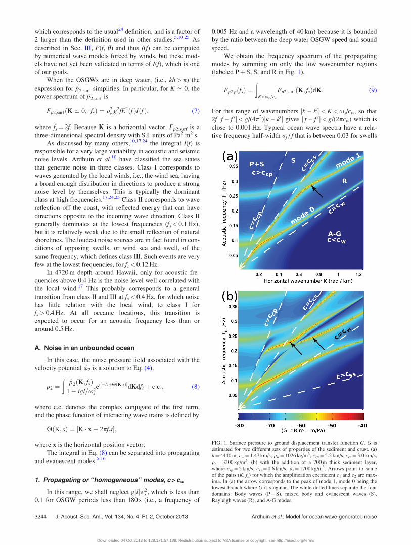
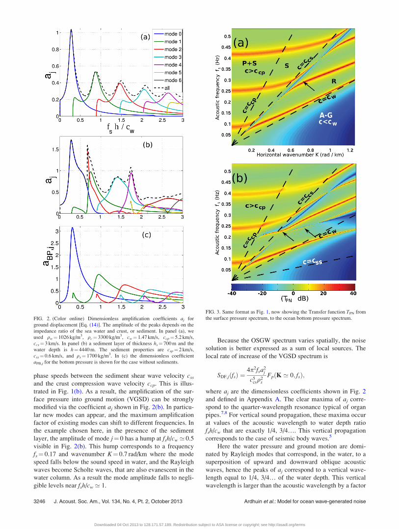
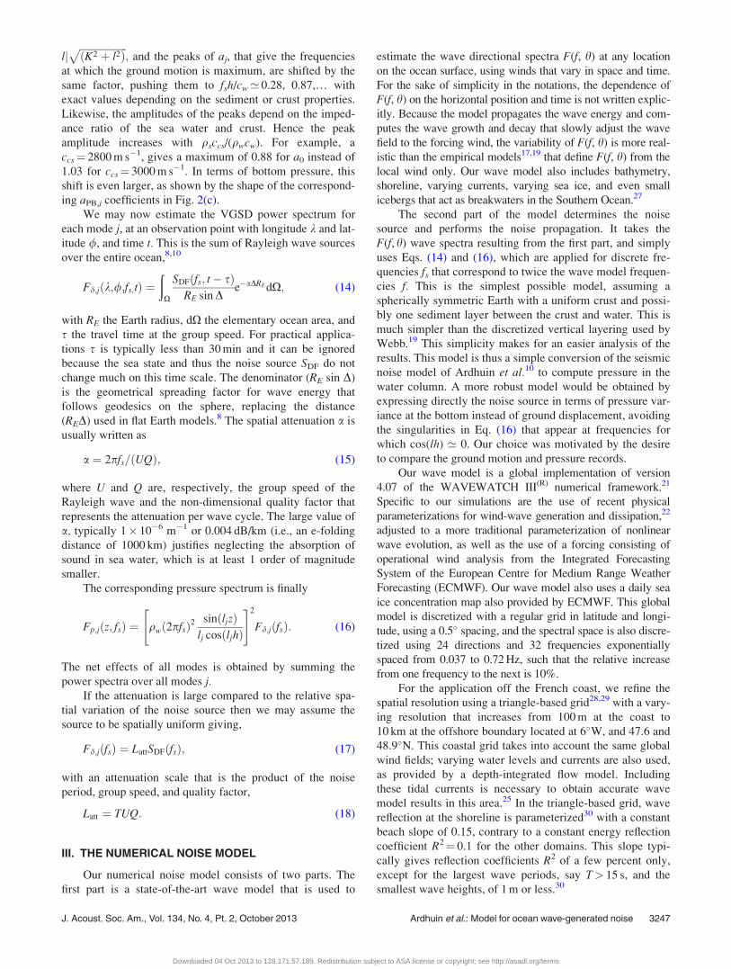
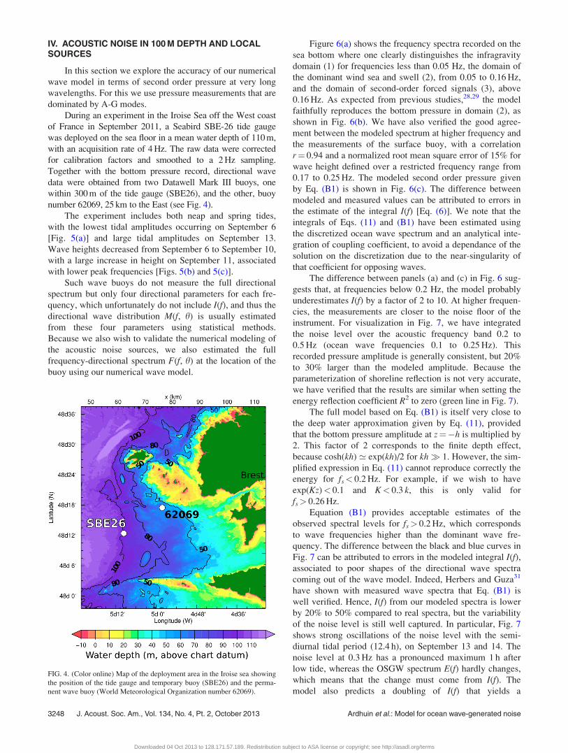
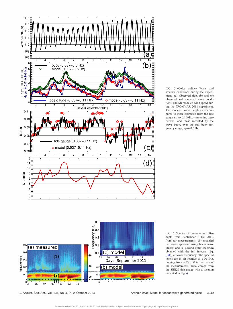
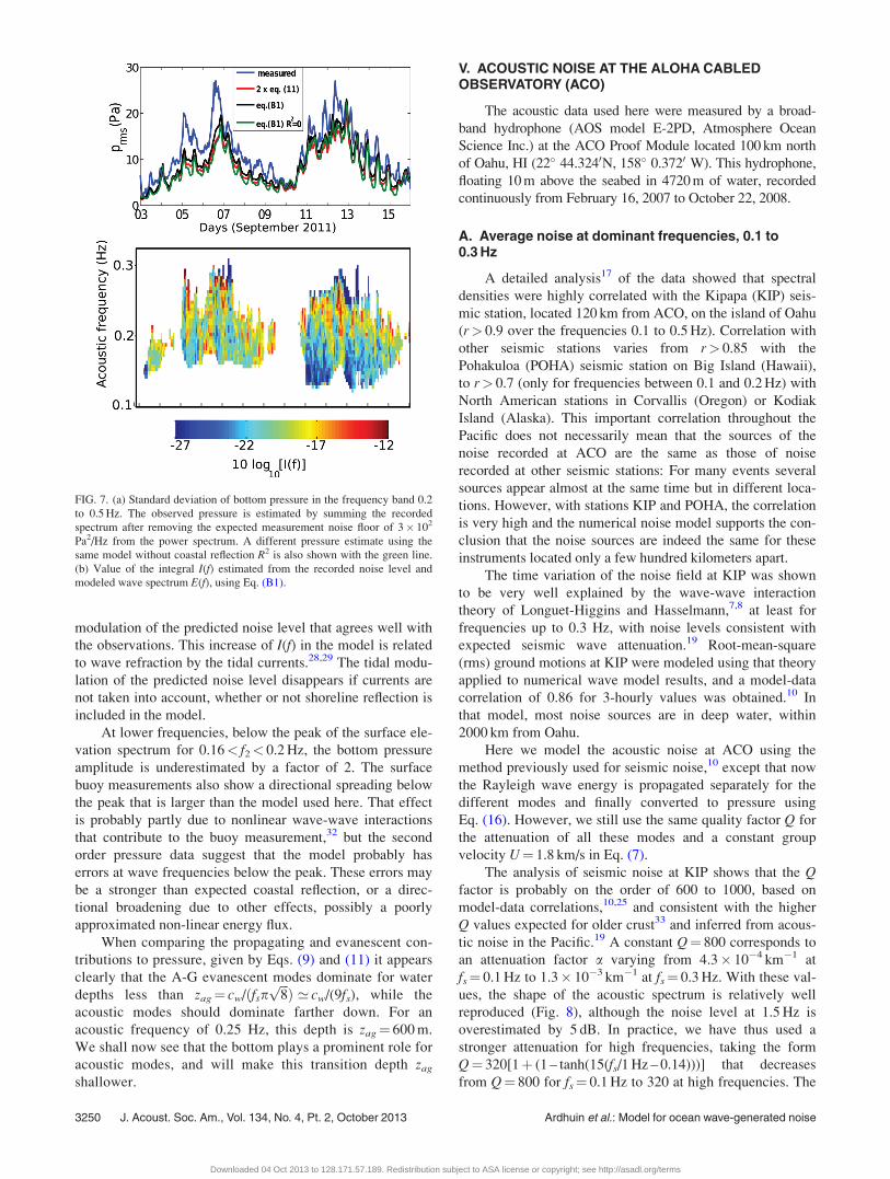
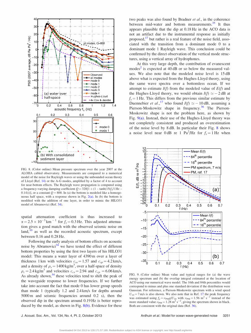
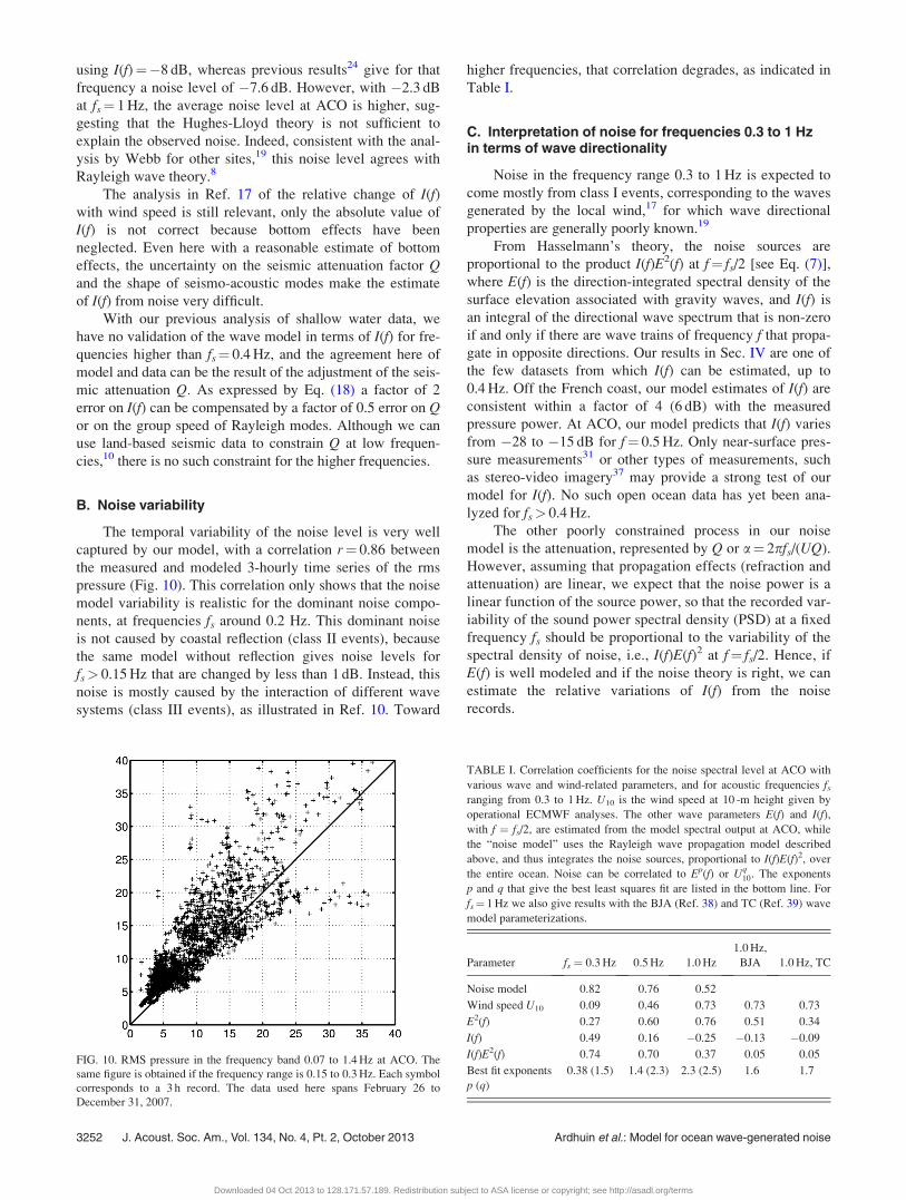
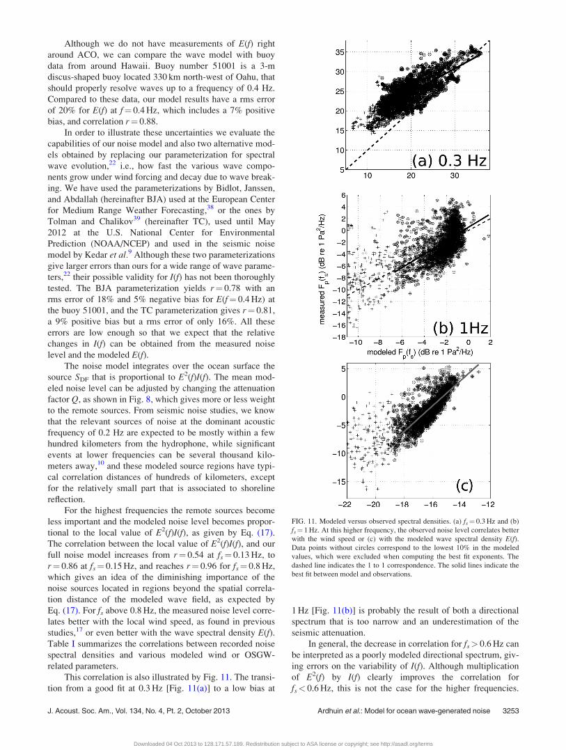
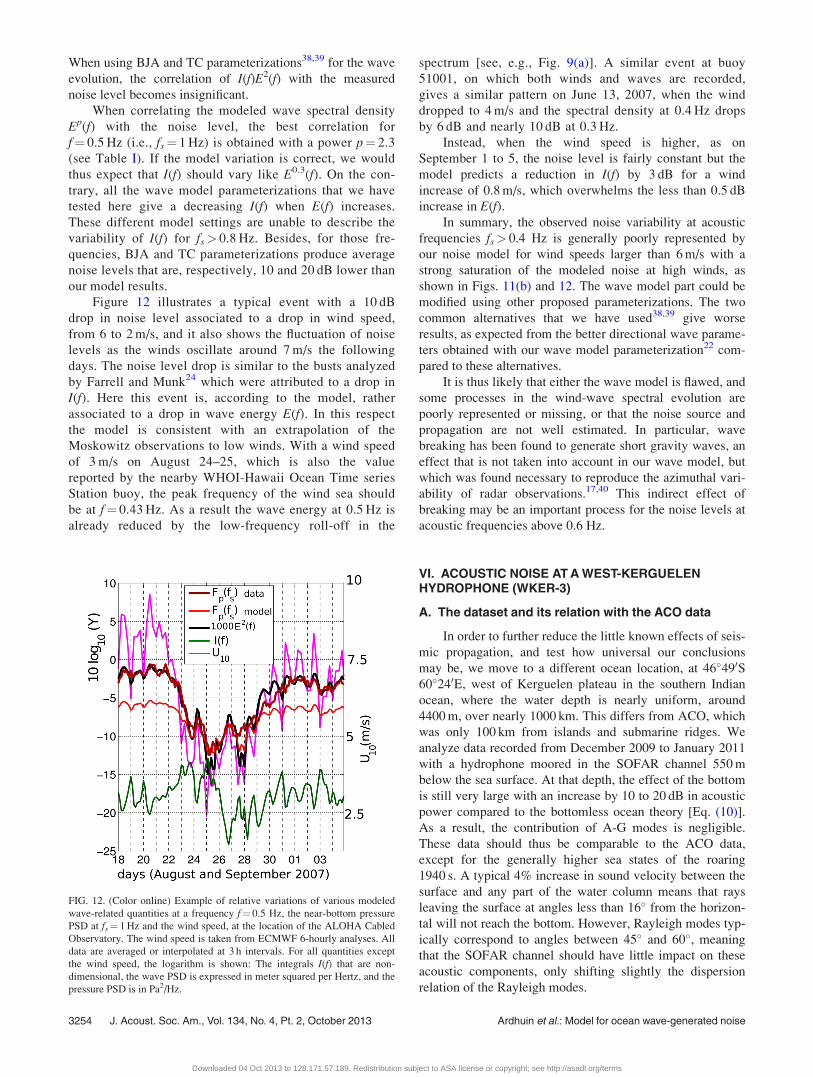
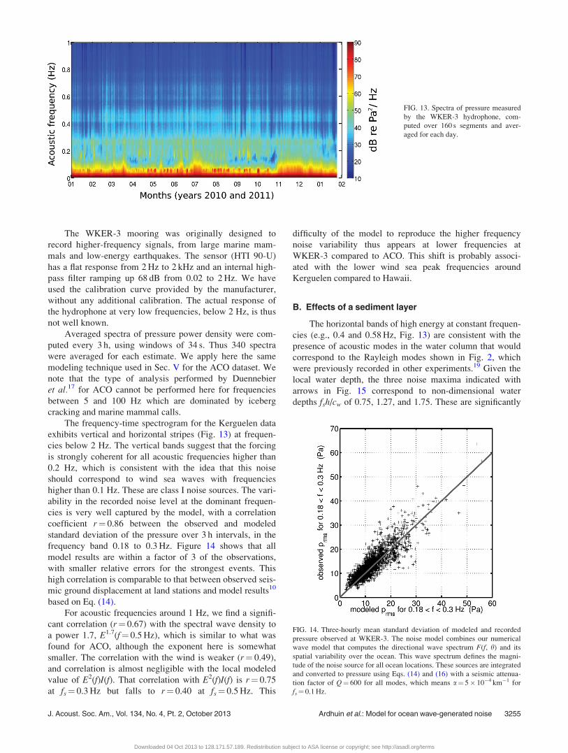
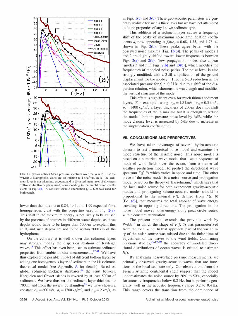
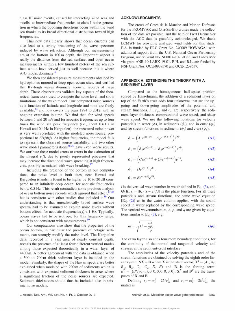

![ALOHA Cabled Observatory Installationaco-ssds.soest.hawaii.edu/Howe_et_al_ACO_Oceans11.pdf · H2O observatories, with improvements based on lessons learned from both [10,13,14], as](https://static.documents.pub/doc/80x56/5ece6a0434278561666573d8/aloha-cabled-observatory-installationaco-ssdssoest-h2o-observatories-with-improvements.jpg)


