1708 IEEE TRANSACTIONS ON MICROWAVE THEORY AND TECHNIQUES, VOL. 37, NO. 11, NOVEMBER 1989

A Numerically Efficient Finite- Element Formulation for the General Waveguide

Problem Without Spurious Modes

Absfruef -A numerically efficient finite-element procedure showing no spurious modes is presented for the analysis of propagation characteristics in arbitrarily shaped metal waveguides loaded with linear materials of arbitrary complex tensor permittivity and permeability. 'lke method is straightforwardly derived from the first-order Maxwell curl equations and comprises both the transversal and longitudinal components of the electric and magnetic fields. Hence, all necessary boundary conditions on the tangential field components are U priori satisfied by the trial functions. With this formulation an absence of spurious modes has been found. Furthermore, by also imposing the additional boundary conditions on the normal components of the magnetic induction and electric displacement fields, the dimension of the resulting matrix equation may be significantly reduced. In this formulation both the propagation constant and the fre- quency may be treated as an eigenvalue of the resulting sparse gened ied eigenvalue problem. For the fundamental modes, both the convergence order and the accuracy of the presented method are found to be signifi- cantly higher than those of comparable methods when applied to some numerical examples.

I. INTRODUCTION HE FINITE-ELEMENT method has been widely used T during the last two decades in the analysis of wave-

guide components [1]-[9]. With this method propagation characteristics of arbitrarily shaped waveguides of differ- ent composition are easily attainable. One drawback that has limited the use of the method, however, has been the spurious (nonphysical) solutions [l], [2], [4], [5] apparent in some of the earlier formulations of the method.

The spurious solutions satisfy the finite-element equa- tions, but not even approximately the original boundary- value problem. The problem can be avoided by the use of a method based on the H-field formulation that is modi- fied by an enforcement of the constraint v.H = 0 on the trial functions [7] (or an analogous E-field version modi- fied by the constraint V - D = 0 [19]). This constraint has been empirically found to suppress the spurious modes present in this formulation. However, the inclusion of the divergence-free constraint increases the numerical com- plexity of the resulting eigenvalue problem by decreasing the matrix sparsity, which is important for the possibility of handling large-size problems in reasonable amounts of time and memory [4], [lo]. The method has recently been

Manuscript received September 19, 1988; revised May 24, 1989. The author is with the Department of Information Technology (FOA3),

Swedish Defence Research Establishment, P.O. Box 1165, S-581 11 Linkijping, Sweden.

IEEE Log Number 8930519.

generalized to lossy problems [9], but is restricted to mate- rials with a scalar permeability, i.e., H a B (or scalar permittivity for the E version, i.e., E a D) .

A different approach, in which the spurious solutions are avoided, is formulated in terms of the transversal field components e, and h, [8]. Here, the spurious modes are found to possess complex propagation constants and may therefore be discriminated when considering propagating modes in nondissipative waveguides.

In this paper a numerically efficient finite-element for- mulation is presented that shows no spurious modes and which may be used to analyze problems involving linear materials of arbitrary complex tensor permittivity and permeability. The method is based on a mixed-field formu- lation [U-[17] comprising both the transversal and longi- tudinal components of E and H . It is straightforwardly derived from the Maxwell curl equations, and as all field components are considered, all the necessary interelement and global boundary conditions on the tangential field components n X E and n x H are easily imposed. The higher number of field components involved in this formu- lation does not necessarily increase the dimension of the final eigenvalue problem (for a given mesh division) as more boundary conditions may be easily imposed on the trial functions. Hence, the continuity of the normal com- ponents of the magnetic induction and electric displace- ment fields ( n . B and n.D) may also easily be imposed, which significantly reduces the final problem size.

On the other hand, in formulations showing spurious modes, some of the necessary global and interelement boundary conditions are not a priori satisfied by the trial functions. In fact, one reported origin of the spurious modes [2] is that some of the tangential boundary condi- tions, which are necessary to unambiguously define the boundary-value problem, are not satisfied. These so-called natural boundary conditions are only guaranteed to be approximately satisfied close to the physically correct solu- tions [ll], [12], but nowhere else. Consequently, spurious solutions may occur, which are not close to any true solution and do not satisfy all the necessary boundary conditions. Two types of spurious solutions may be imag- ined: one type that satisfies the natural boundary condi- tions in a wide mean-value sense (as a sum of integrals along the boundary of each element), but pointwise unfor-

0018-9480/89/1100-1708$01.00 01989 IEEE

SVEDIN: A NUMERICALLY EFFICIENT FINITE-ELEMENT FORMULATION 1709

tunately not even approximately [2, p. 5561, and another type that does not satisfy the natural boundary conditions even in the wide mean-value sense, and hence not the Maxwell equations within each element.

Numerical examples, using both rectangular and trian- gular first-order elements, are given for rectangular wave- guides loaded with dielectric slab, lossy dielectric, and lossy anisotropic slab and for a circular hollow waveguide. In none of these cases have spurious modes been found, and the accuracy for the fundamental modes and the convergence rate of the eigenvalue are found to be very high when compared to the magnetic-field [7] , [9] and the transversal-field formulations [8]. For the first-order rect- angular and triangular elements considered in this paper, < 6 N and between 3N and 6 N unknowns are required, respectively, for N elements to be compared e.g. with exactly 8 N and 6 N unknowns, respectively, required in the transversal field formulation [8]. Furthermore, by matrix manipulations of the resulting eigenvalue problem, the problem dimension may be reduced up to 300 percent, but with decreased matrix sparsity as a result.

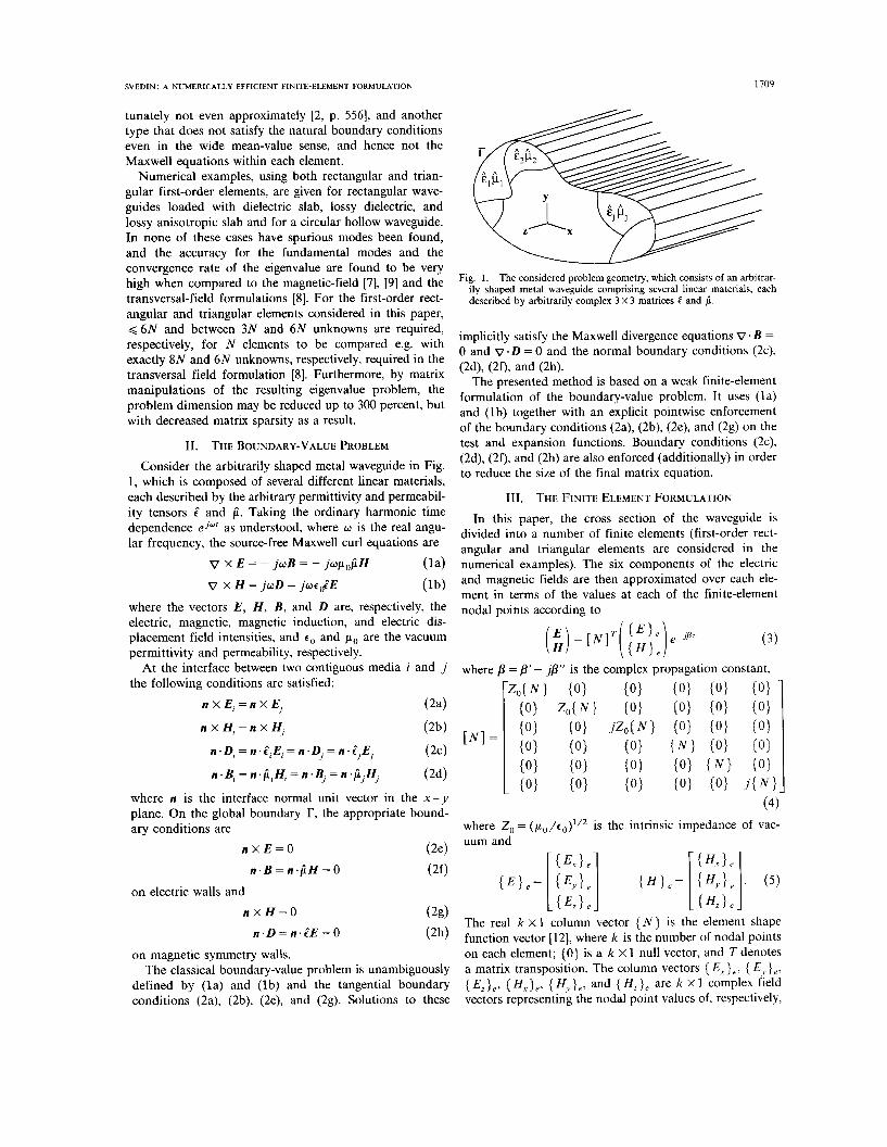
11. THE BOUNDARY-VALUE PROBLEM Consider the arbitrarily shaped metal waveguide in Fig.

1, which is composed of several different linear materials, each described by the arbitrary permittivity and permeabil- ity tensors E^ and f i . Taking the ordinary harmonic time dependence elw' as understood, where w is the real angu- lar frequency, the source-free Maxwell curl equations are

v x E = - j o B = - j w p O W (14 v X H = jwD = jocoE^E (1b)

where the vectors E , H , B , and D are, respectively, the electric, magnetic, magnetic induction, and electric dis- placement field intensities, and c o and po are the vacuum permittivity and permeability, respectively.

At the interface between two contiguous media i and j the following conditions are satisfied:

n X E, = n X EJ

n X H, = n X HJ

( 2 4

(2b)

n . Dl = n . ;,E, = n .DJ = n ?JEJ (2c)

n . B , = n . f i , H , = n . B J = n . f i J H J ( 2 4

where n is the interface normal unit vector in the x - y plane. On the global boundary r, the appropriate bound- ary conditions are

n X E = O ( 2 4

(2f)

n X H = O (2g)

n . D = n - E E = O (2h)

n - B = n-f iH = 0

on electric walls and

on magnetic symmetry walls. The classical boundary-value problem is unambiguously

defined by (la) and (lb) and the tangential boundary

Fig. 1. The considered problem geometry, which consists of an arbitrar- ily shaped metal waveguide comprising several linear materials, each described by arbitrarily complex 3 x 3 matrices P and j i .

implicitly satisfy the Maxwell divergence equations V. B =

0 and V - D = 0 and the normal boundary conditions (2c),

The presented method is based on a weak finite-element formulation of the boundary-value problem. It uses (la) and (lb) together with an explicit pointwise enforcement of the boundary conditions (2a), (2b), (2e), and (2g) on the test and expansion functions. Boundary conditions (2c), (2d), (20, and (2h) are also enforced (additionally) in order to reduce the size of the final matrix equation.

(24, (20, and (2h).

111. THE FINITE ELEMENT FORMULATION

In t h s paper, the cross section of the waveguide is divided into a number of finite elements (first-order rect- angular and triangular elements are considered in the numerical examples). The six components of the electric and magnetic fields are then approximated over each ele- ment in terms of the values at each of the finite-element nodal points according to

(3)

where Z , = (po/co)1'2 is the intrinsic impedance of vac- uum and

( E x ) e { H A

w e = [ ;;Ij we= [ w j. ( 5 )

The real k x 1 column vector { N } is the element shape function vector [12], where k is the number of nodal points on each element; {0} is a k x 1 null vector, and T denotes a matrix transposition. The column vectors {E,}, , { E , . } e , { E , } , , { H , } , , { H,},, and { H 2 } , are k x 1 complex field vectors remesentine the nodal Doint values of, respectively, conditions- (2a), (2b), (2e), and (2g). Solutions to these ... ~~ "

1710 IEEE TRANSACTIONS ON MICROWAVE THEORY AND TECHNIQUES, VOL. 37, NO. 11, NOVEMBER 1989

E,/Zo, E.,/Z,, - jEz/Zo, H,, H,, and - jH, on each element.

The finite-element solutions E and H are weak solu- tions [12, ch. 41 of (la) and (lb) which should satisfy

+ H,,*,,.( - j v X E + wp,,fiH)) d x d y = 0 ( 6 )

for all admissible test functions E,,,, and Htest where the appropriate boundary conditions are handled during the summation C over all elements [ll]. Here, the necessary continuity requirements (2a), (2b), (2e), and (2g) on n X E and n X H are explicitly imposed, but also the additional requirements (2c), (2d), (29, and (2h) on n . B and n . D are enforced.

Using a Galerkin procedure with the finite-element ex- pansion (3) for both trial and test functions, there results the following generalized eigenvalue problem:

where the column vector is composed of all the unknown nodal point parameters used to represent E and H in the waveguide and either p or w may be treated as the eigenvalue. By writing (la) and (lb) in component form, the quadratic sparse matrices [PI, [ Q], and [RI are found to be

[cl = { N I a { N ) T / J Y . (13)

By solving the eigenvalue problem (7), all field compo- nents for the approximate fields of different eigenmodes in the waveguide are directly determined and the correspond- ing eigenvalues j3 (or U ) are found.

For loss-free waveguides the regular matrix [PI is Her- mitian and real for the usual cases, such as dielectrics and transversely magnetized ferrites. The singular matrices [ Q] and [RI are always Hermitian.

For resonator problems or the calculation of dispersion relations in problems with frequency-independent loss-free materials, it is advantageous to treat the frequency w as the eigenvalue, because (7) may then be reformulated as a standard eigenvalue problem, which is Hermitian. Then, very efficient sparse eigenvalue routines are available [lo],

The boundary conditions have been taken care of by solving (2a)-(2h) for each nodal point [18]. As an example, consider the arbitrary internal node point j (using triangu- lar elements) shown in Fig. 2. The boundary conditions (2a)-(2h) then require the enforcement of

~ 4 1 .

n, X E, = n, X EiPl n, X Hi = n, X

(144

(14b) where the El's and Hi's represent the values of the electric

d x dy

SVEDIN: A NUMERICALLY EFFICIENT FINITE-ELEMENT FORMULATION 1711

Fig. 2. The geometry at the internal node point j , in an arbitrary triangular-element mesh. Generally, the elements contain different materials, each described by constant matrices <, and jl,, i = 1,2, . . . , r .

and magnetic fields, respectively, at the node point j in the element i , and the subscript i runs cyclically modulo r from 1 to r . In t h s paper, the additional enforcements of

nI . i lE , = n r - P , p l E , - l (144 n;f i ,H, = n,-fi,-lH,pl (144

are also made. At the external boundary r one obtains similar homogeneous equations for the global boundary conditions (2e)-(2h) to be satisfied (perfect electric and magnetic conductors).

Using (14a)-(14d), it can be concluded that the total number of unknowns is G 6 N p , where Np is the number of nodal points. This yields for the first-order rectangular elements < 6 N unknowns, where N is the number of elements. For comparison, the transversal-field method uses 8 N unknowns for the same type of elements. For the first-order triangular elements, the required number of unknowns depends on the mean number of nodal points per triangle, but lies in the range 3N to 6 N , to be com- pared with exactly 6 N for the transversal-field formula- tion [ S I .

To further demonstrate the difference between the method outlined here and the earlier formulations with regard to the fulfillment of boundary conditions, one should note that the dimension of the eigenvalue problem (7) may be reduced by rewriting it in terms of fewer parameters (field components). As an example, write (7) with P as eigenvalue in detailed matrix form:

[P3I [ p 4 I [R2I [OI

[R4I [OI [ p 7 I [P,I [OI [R31 RI [P,l

where the [P,]'s, [Q,]'s, and [R,]'s are submatrices of w [ P ] ,

[ Q ] , and [RI, respectively (see the Appendix), and the column vectors { E t } , { E L } , { H I } , and { Hz } are parame- ters used to represent, respectively, the transversal electric, longitudinal electric, transversal magnetic, and longitudi- nal magnetic field components for the global assembly of finite elements. Some elementary matrix algebra applied to (15) yields the following eigenvalue problem:

where

t A I = t p13 - p 2 I t p4 3 - t P3 3 - I R13 t p* I - t R 4 I (1 7 4

PI = - t P 2 1 [ ~ 4 l - ' [ & I - [RlI[~8I- '[P71 07b)

[cl = -[R,I[p41-'[&1- [P,l[p8l-'[R41 (174

[ol = P S I - [R,I[P4I-'[R21- [P,I[~81p1[P71 (174 whch is a generalized eigenvalue problem of approxi- mately 2/3 the order of the original problem (7) and only comprising parameters related to the transversal field com- ponents of E and H . Observe that in (16 ) all the necessary tangential boundary conditions are explicitly fulfilled (and additionally also the normal conditions); this is to be compared with [SI, where the conditions on the longitudi- nal components are ignored. For all isotropic cases and the special anisotropic cases where only ex,,, e y x , pxy, and pyx # 0, the matrices [ P2], [ P,], [ P,], and [ P,] become zero with vanishing [B] and [C] as a result. In this case (16 ) may be reduced to either one of the two following eigen- value problems:

( t 1 - P Q 2 1 [ A 1 - '[ Q1 I ) { HI 1 = 0 (18a)

([AI - P 2 [Q,] [ D1 p 1 [ Q 2 1 ) { E, 1 = 0 (18b) each of dimension only approximately 1 / 3 that of (7) and expressed in parameters related to transversal H or transversal E only. Again observe that in (18a) and (18b) all the boundary conditions on the tangential components are incorporated, and additionally also the normal condi- tions. Equation (18a) has been investigated, and found to produce the same eigensolutions as (7) (using the rela- tions between the field components used to obtain (18a) from (7)).

The most important numerical property of the eigen- value problem (7) is, however, the 0 ( 1 / N ) sparsity of the matrices, which means that the number of nonzero matrix elements on each row is almost independent of the dimen- sion N . For large-size problems sparse eigenvalue codes may be used on (7), whch will save a significant amount of CPU time and memory [lo]. As more compact forms of (7) as (16) , (18a), or (18b) are less sparse, it may be preferable to use (7), despite the roughly 300 percent reduction of unknowns in, for instance, (18b).

IV. NUMERICAL EXAMPLES In this section examples where analytical solutions exist

[13] are studied in order to demonstrate the strength of the present method. In this paper first-order rectangular and triangular elements are used. In order to easily obtain both

IEEE TRANSACTIONS ON MICROWAVE THEORY AND TECHNIQUES, VOL. 37, NO. 11, NOVEMBER 1989

Exact solution [ 131 . Present method

E= 2.25

I I -2a-

I I 2 koa 3

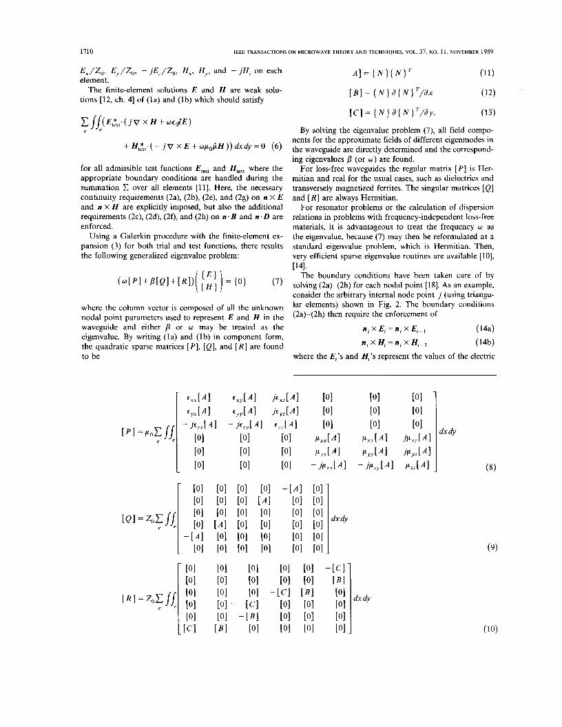
The normalized disDersion relations for the fundamental TE, Fig. 3. and higher order LSM,, mbdes in the dielectric-slab-loaded rectangular waveguide (inset). The finite-element division is 4x8 for both finite- element solutions.

eigenvectors and eigenvalues, the complex generalized eigenvalue problem routine NAG F02GJF (in double pre- cision) is used [14]. With this routine, all the eigenvalues and eigenvectors of (7) are given but the matrix sparsity is not considered and consequently the more compact forms (16) or (18) would probably be faster to execute despite the necessary matrix inversions involved. As pointed out else- where [4], [lo], the use of sparse matrix routines will considerably reduce the amount of storage and computa- tional time needed to solve (7). In fact, for very large problems, even on a supercomputer, the sparsity of the eigenvalue problem will be of decisive importance.

A . Dielectric Slab in Rectangular Waveguide As a first example [8], a rectangular waveguide inhomo-

geneously loaded with a dielectric slab is considered. In Fig. 3 the calculated and exact [13] dispersion relations for the fundamental TE,, and the higher order LSM,, mode are gwen for a waveguide of dimensions a X 2 a loaded at one end with a dielectric slab of dimensions a x a and relative permittivity z = 2.25. The cross section was divided into 4 x 8 = 32 elements (6 x 32 = 192 variables). For com- parison, the transversal field (e, - h t ) method [ 81 was coded using the same type of elements. For this structure using the same division for both methods, the present method is more accurate, as is obvious from the dispersion relation of the LSM,, mode, and for both modes the present method shows an error at least one order of magnitude smaller (in [ 81 a similar accuracy with the transversal-field method is obtained using 64 first-order triangular ele- ments).

A property of considerable importance in any finite-ele- ment method is the convergence of the solution as the problem size increases. Here, the convergence rate, m, of the relative error, e , of the propagation constant as a function of the number of nodal points, Np, in the finite-

10’ Present method - Formulation [8]

,n 4 t I O 1 lo2 NP 10’

I U

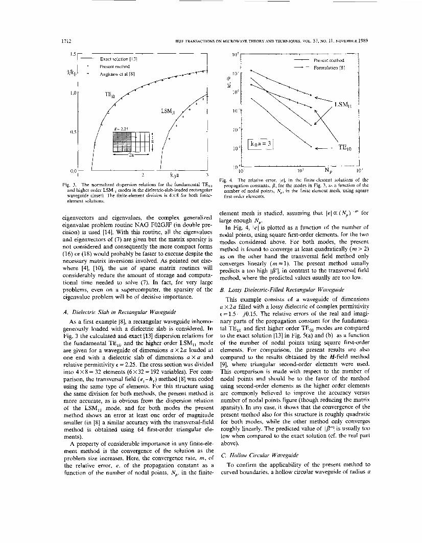
Fig. 4. The relative error, le\, in the finite-element solutions of the propagation constants, p , for the modes in Fig. 3, as a function of the number of nodal points, N p , in the finite-element mesh, using square first-order elements.

element mesh is studied, assuming that (el a (N, ) -” for large enough Np.

In Fig. 4, (el is plotted as a function of the number of nodal points, using square first-order elements, for the two modes considered above. For both modes, the present method is found to converge at least quadratically ( m > 2) as on the other hand the transversal field method only converges linearly ( m = 1). The present method usually predicts a too high 1/3’1, in contrast to the transversal field method, where the predicted values usually are too low.

B. Lossy Dielectric-Filled Rectangular Waveguide

This example consists of a waveguide of dimensions a X 2a filled with a lossy dielectric of complex permittivity z =1.5- j0.15. The relative errors of the real and imagi- nary parts of the propagation constant for the fundamen- tal TE,, and first hgher order TE,, modes are compared to the exact solution [13] in Fig. 5(a) and (b) as a function of the number of nodal points using square first-order elements. For comparison, the present results are also compared to the results obtained by the H-field method [9], where triangular second-order elements were used. T h s comparison is made with respect to the number of nodal points and should be to the favor of the method using second-order elements as the higher order elements are commonly believed to improve the accuracy versus number of nodal points figure (though reducing the matrix sparsity). In any case, it shows that the convergence of the present method also for t h s structure is roughly quadratic for both modes, whle the other method only converges roughly linearly. The predicted value of IP”I is usually too low when compared to the exact solution (cf. the real part above).

C. Hollow Circular Waveguide To confirm the applicability of the present method to

curved boundaries, a hollow circular waveguide of radius a

SVEDIN: A NUMERICALLY EFFICIENT FINITE-ELEMENT FORMULATION 1713

10‘:

l o Z :

10’:

10‘

i

E = 1 5 - ~ 1 5 :

1 -a- 1 I ”

10’ NP 10‘ lo?

(a)

10‘ ; Present method I

10‘

10“ I O ’ IO‘ NP 10’

(b)

Fig. 5. (a) The relative error in the finite-element solutions of the real part of the propagation constant, /3’, for the fundamental TE,, and the higher order TE,, modes in the lossy dielectric-loaded rectangular waveguide (inset) as a function of the number of nodal points, using square first-order elements. (b) The relative error in the imaginary part, 8”. of the propagation constant corresponding to errors in the real part shown in Fig. 5(a).

is analyzed using first-order triangular elements. Disper- sion relations for the three lowest propagating modes are given in Fig. 6. In th s example, one quarter of the wave- guide has been divided into 36 first-order ordinary triangu- lar elements utilizing the inherent symmetry for the differ- ent modes. The accuracy of the hgher order modes can, of course, be improved by increasing the number of elements or by using higher order interpolation on each element. Thus, the applicability of the present method is also demonstrated for the case of curved boundaries, and the accuracy is shown to be retained when using the triangular finite elements.

Also for this case, predicted values of IP’I and I@’’[ are usually found to be, respectively, too high and too low. This is analogous to a prediction of p 2 that is too high or, equivalently, a prediction of the transversal wavenumber k; that is too low. A disadvantage related to th s fact is

I A b ’ Present method ’ Present method

I

0.0 1 1 2 3 koa 4

Fig. 6. The propagation characteristics of a hollow circular waveguide, as obtained by the presented method using a mesh (inset) consisting of 36 first-order elements. At the external boundary, r, the normal magnetic induction field, Br, and the tangential electric field, E,+ and .Ez, are forced to vanish.

that some of the higher order modes, which actually are cut off, are predicted to have I/?’/ > 0, and thus get mixed with the propagating modes in the calculated P’(o) spec- trum. However, the former modes seem to be identified by possessing normalized residuals, according to (1 a) and (lb), which are higher than for the latter modes.

D. Anisotropic Slab with Dielectric and Magnetic Losses As a more advanced example relating to the material

properties, an anisotropic slab with both dielectric and magnetic losses is studied to verify the general validity of the present method. It consists of a rectangular waveguide of dimensions a X 2a loaded at one end with an anisotropic slab of dimensions a X a. The slab has the relative scalar permittivity 6 = 2 - j0.2 and the relative tensor permeabil- ity

1- j0 . l 0 0.05- j0.5 1- j0 . l

1- j0 . l -0.05+ j0.5 0

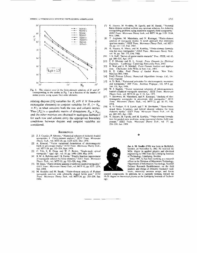
For the fundamental TE,, and higher order TE,, modes, a division in 1 X 8 first-order elements gives the complex dispersion relations shown in Fig. 7, where the exact solutions, attainable from the characteristic equation in [13], also are plotted. The correspondence is very good along the whole frequency axis. Note that only eight first-order rectangular elements are used for both the real and imaginary parts of the propagation constants.

The corresponding convergence rates are found in Fig. 8, where square first-order elements have been used to calculate the relative errors in the real and imaginary parts of the complex propagation constant, for modes propagat- ing in both the positive and negative z direction. The resulting convergence order is approximately m = 2.5 for both modes.

1714 IEEE TRANSACTIONS ON MICROWAVE THEORY AND TECHNIQUES, VOL. 37, NO. 11. NOVEMBER 1989

Present method TElO

Present method TE20

- Exact solution [13]

I * , I -2a- -U

0 1 2 koa 3

Fig. 7. Complex propagation characteristics for the fundamental TE!, and higher order TE2,) modes in the magnetically anisotropic, magneti- cally and electrically dissipative slab-loaded rectangular waveguide (inset). The + and - indices denote modes propagating in, respec- tively, the positive and negative z directions.

V. CONCLUSION An advantageous finite-element method for the metal

waveguide problem has been developed by which complex propagation characteristics may be obtained for arbitrarily shaped waveguides of arbitrary composition. The method is based on a straightforward application of the Galerkin method to the first-order Maxwell curl equations and comprises all six field components of the electric and magnetic fields. All the necessary boundary conditions on the tangential field components, and additionally on the normal components, are enforced, thus making the final problem size of the same order, or lower, than for compa- rable formulations.

With the presented method, no spurious modes have been observed, and it has been found to possess very good accuracy and convergence properties in a number of exam- ples that have been analyzed using both rectangular and triangular first-order finite elements. Especially when using the first-order triangular elements, high-order cutoff modes are found with real propagation constants, as the square of the propagation constant is usually predicted too high with the present formulation. However, by calculating the nor- malized residuals of the solutions, the modes of interest seem to be identified as having the smallest residuals, and are hence separated from the ones with larger residuals.

A very important property of the presented formulation is that the resulting eigenvalue problem is of the sparse type, suitable for large-size problems, and that it is possi- ble to treat both the propagation constant and the fre-

may be reformulated in terms of fewer than six field components, and for some usual cases, the final problem size may be reduced by a factor of up to 3.

The extension to higher order elements is straightfor- ward, and by modifications of the method it is possible to treat other types of waveguides as well, e.g. dielectric waveguides with impedance walls and open unbounded dielectric waveguides properly treating the region of infin- ity.

APPENDIX

The submatrices in (14) are found from (8)-(10) to be

where the handling of boundary conditions, inherent in each summation symbol, depends on the origin of each of the submatrices in @)-(lo), i.e., on the relation between local and global variables obtained from (2a)-(2h). Thus, - - -

quency as an eigenvalue. The resulting matrix equation C, in (A8) should incorporate the boundary conditions

1715 SVEDIN: A NIJMERICALLY EFFICIENT FINITE-ELEMENT FORMULATION

‘ O 2 1

- TElO B’+ TElO B”+ TElO E- E l 0 B”- - TE20 B’+ TE20 o”+ TE20 8’- TE20 B”-

..... ~ ....

... .+. . ---*--

..... ~ ....

.... x- .... ___I__

h I O I

10’ NP I O ’ I O 2

Fig. 8. The relative error in the finite-element solutions of 8’ and /3” corresponding to the modes in Fig. 7 as a function of the number of nodal points, using square first-order elements.

relating disjoint [ll] variables for H, (4N if N first-order rectangular elements) to conjoint variables for H , ( = NHz = N ) , in what concerns both the row and column entries. Thus [P,] is a quadratic matrix of dimensions NHz X NHz, and the other matrices are obtained in analogous fashion if for each row and column entry the appropriate boundary conditions between disjoint and conjoint variables are considered.

REFERENCES Z. J. Csendes, P. Silvester, “Numerical solution of dielectric loaded waveguides: I -Finite-element analysis,” IEEE Trans. Microwave Theory Tech.. vol. MTT-18, pp. 1124-1131, Dec. 1970. A. Konrad, “Vector variational formulation of electromagnetic fields in anisotropic media,” IEEE Trans. Microwave Theory Tech., vol. MTT-24, pp. 553-559, Sept. 1976. C. Yeh, S. B. Dong, and W. P. Brown, “Single-mode optical waveguide,” Appl. Opt., vol. 18, pp. 1490-1504, May 1979. B. M. A. Rahman and J. B. Davies, “Penalty function improvement of waveguide solution by finite elements,” IEEE Trans. Microwave Theory Tech., vol. MTT-32, pp. 922-928, Aug. 1984. M. Hano, “Finite-element analysis of dielectric-loaded waveguides,” IEEE Trans. Microwave Theory Tech., vol. MTT-32, pp. 1275-1279, Oct. 1984. M. Koshiba and M. Suzulu, “Finite-element analysis of If-plane waveguide junction with arbitrarily shaped ferrite post,” IEEE Trans. Microwave Theorv Tech.. vol. MTT-34. D D . 103-109. Jan.

K. Hayata, M. Koshiba, M. Eguchi, and M. Suzuki, “Vectorial finite-element method without any spurious solutions for dielectric waveguiding problems using transverse magnetic-field component,” IEEE Trans. Microwave Theory Tech., vol. MTT-34, pp. 1120-1124, Nov. 1986. T. Angkaew, M. Matsuhara, and N. Kumagai, “Finite-element analysis of waveguide modes: A novel approach that eliminates spurious modes,’’ IEEE Trans. Microwave Theory Tech., vol. MTT- 35, pp. 117-123, Feb. 1987. K. Hayata, K. Miura, and M. Koshiba, “Finite-element formula- tion for lossy waveguides,” IEEE Trans. Microwave Theoql Tech., vol. 36, pp. 268-275, Feb. 1988. I. S. Duff, “Survey of sparse matrix research,” Proc. IEEE, vol. 65, pp. 500-535, Apr. 1977. P. P. Silvester and R. L. Ferrari, Finite Elements /or Electrical Engineers. R. Wait and A. R. Mitchell, Finite Element Analysis and Applicu- tions. R. E. Collin, Field Theory of Guided Waves. New York: McGraw-Hill, 1960. NAG Fortran Library, Numerical Algorithms Groups Ltd., Ox- ford, England. A. D. Berk, “Variational principles for electromagnetic resonators and waveguides,” IRE Trans. Antennas Propagat., vol. AP-4, pp. 104-111, Apr. 1956. W. J. English, “Vector variational solutions of inhomogeneously loaded cylindrical waveguide structures,” IEEE Trans. Microwave Theory Tech., vol. MTT-19, pp. 9-18, Jan. 1971. Y. Satomura, M. Matsuhara, and N. Kumagai, “Analysis of elec- tromagnetic waveguides in anisotropic slab waveguides,” IEEE Trans. Microwave Theory Tech., vol. MTT-22, pp. 86-92, Feb. 1974. K. D. Paulsen, D. R. Lynch, and T. W. Strohbehn, “Three-dimen- sional finite, boundary, and hybrid element solution for lossy dielectric media,” IEEE Trans. Microwave Theory Tech., vol. 36, pp. 682-693, Apr. 1988. K. Hayata, M. Eguchi, and M. Koshiba, “Finite-element formula- tion for guided-wave problems using transversal electric field com- ponent,” IEEE Trans. Microwave Theory Tech., vol. 37, pp. 256-258, Jan. 1989.

Cambridge: Cambridge University Press, 1983.

Chichester: John Wiley & Sons Ltd., 1985.

Jan A. M. Svedin (S’88) was born in Skelleftei, Sweden, on November 4, 1962. He received the MSc degree in applied physics and electrical engneering in 1986 from the Linkoping Institute of Technology, Linkoping, Sweden.

Since 1987, he has been working as a research officer in the Division of Mmowave Technology, Department of Information Technology, Swedish Defence Research Establishment, on the field analysis and design of dielectric resonator osc~l- lators, microstrip antenna arrays, and ferrite

control components In addition, he is currently worlung toward the Ph D degree In theoretical physics at the Linkoping Institute of Technol-

1986.