A 'parareal' in time discretization of differential … Introduction Algorithm Stability for ODE...

Outline Introduction Algorithm Stability for ODE schemes Applications to PDEs Numerical experiments Concluding remarks

A ”parareal” in time discretization of di↵erentialequations

Yang Yang

Division of Applied Math Brown University

April 26, 2012


Outline

1 Introduction

2 Algorithm

3 Stability for ODE schemes

4 Applications to PDEs

5 Numerical experiments

6 Concluding remarks


Outline

1 Introduction

2 Algorithm









Parallel in time?

How to obtain the solution at time level n + 1 without knowing thesolution at time level n?

prediction

correction


Parallel in time?


prediction

correction


Parallel in time?


prediction

correction


The parareal algorithm was first presented by Lions, Madayand Turinici in 2001, as a numerical method to solve evolutionproblem in parallel.

An improved version was presented by Bal and Maday in2002. Further improvements and understanding, as well asnew applications of the algorithm, were presented by Ba�coet al. and Maday and Turinici in 2002.

In 2003, the stability of the algorithm for ODE schemes wasanalyzed.

In 2003, the stability and convergence of the pararealalgorithm to PDEs were given.

















Applications

The method can be applied to the pricing of an Americanoption, and molecular-dynamics.

The algorithm has received a lot of attention in the domaindecomposition literature.

Extensive experiments can be found for fluid and structureproblems, N-S equations, and for reservoir simulation.


Applications





Applications





Outline

1 Introduction

2 Algorithm






model equation

Consider the following ODE

⇢dy

dt

(t) = �µy(t) t 2 [0,T ],y(t = 0) = y0.

We decompose the time interval [0,T ] into N subintervals[T n,T n+1] of size �T = T/N.


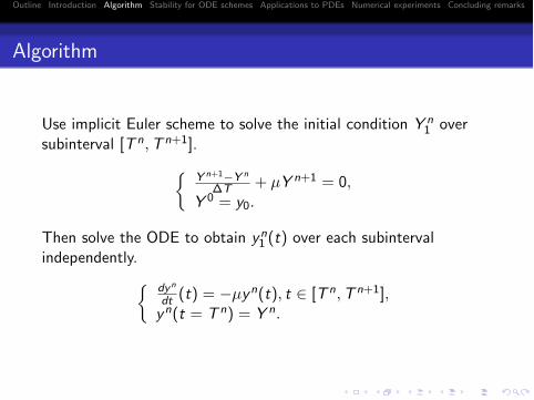
Algorithm

Use implicit Euler scheme to solve the initial condition Y n

1 oversubinterval [T n,T n+1].

⇢Y

n+1�Y

n

�T

+ µY n+1 = 0,Y 0 = y0.

Then solve the ODE to obtain yn

1 (t) over each subintervalindependently.

⇢dy

n

dt

(t) = �µyn(t), t 2 [T n,T n+1],yn(t = T n) = Y n.


Improve the accuracy iteratively from Y n

k

and yn

k

(t) as follows:

Introduce the jumps Sn

k

= yn�1k

(T n)� Y n

k

.

Propagate the jumps with a coarse resolution of the �n

k

,

(�n+1k

��n

k

�T

+ µ�n+1k

=S

n

k

�T

,�0k

= 0.

Y n

k+1 = yn�1k

(T n) + �n

k

.



k

and yn

k

(t) as follows:


k

= yn�1k

(T n)� Y n

k

.


k

,

(�n+1k

��n

k

�T

+ µ�n+1k

=S

n

k

�T

,�0k

= 0.

Y n

k+1 = yn�1k

(T n) + �n

k

.



k

and yn

k

(t) as follows:


k

= yn�1k

(T n)� Y n

k

.


k

,

(�n+1k

��n

k

�T

+ µ�n+1k

=S

n

k

�T

,�0k

= 0.

Y n

k+1 = yn�1k

(T n) + �n

k

.


A modified scheme

The parareal algorithm is then given as the predictor-correctorscheme

yn

k

= G�T

(yn�1k

) + F�T

(yn�1k�1 )� G�T

(yn�1k�1 ),

where F�T

is the fine propagator while G�T

is the coarsepropagator.


Outline

1 Introduction

2 Algorithm






Considery 0 = �µy

with suitable initial condition.Explicit Euler method

yn

= yn�1 ��Tµy

n�1 = (1��Tµ)ny0 = R(µ�T )ny0.

Implicit Euler methods

yn

= yn�1 ��Tµy

n

= (1 + �Tµ)�ny0 = R(µ�T )ny0.

R(µ�T ) 1 will prevent the numerical schemes from blowing upfor increasing n.


Assume s = �T

dt

,

yn

k

= R(µ�T )yn�1k

+ r s(µdt)yn�1k�1 � R(µ�T )yn�1

k�1 ,

where r(µdt) is the stability function for the fine propagator F�T

while R is that of G�T

. Denote r = r s , we obtain

yn

k

= Ryn�1k

+ (r � R)yn�1k�1 .

Therefore,

yn

k

=

kX

i=0

✓ni

◆(r � R)iRn�i

!y0.


The ”stability function” for the Parareal scheme

H =

kX

i=0

✓ni

◆(r � R)iRn�i

!.

|H| (|r � R|+ |R|)n 1.

We want |r � R � R| 1 and |r � R + R| 1, therefore

r � 1

2 R r + 1

2.


Outline

1 Introduction

2 Algorithm






Assumptions

G�T

is Lipschitz and an approximation of order m

supn

||G�T

(T n, u)� G�T

(T n, v)||B0 (1 + C�T )||u � v ||

B0 ,

supn

||G�T

(T n, u)� F�T

(T n, u)||B0 C (�T )m+1||u||

B1 .

The above yields

||y(TN)� yN

1 ||B0 C (�T )m||y0||B1


Assumptions cont.

||u(t)||B

j

C ||u(0)||B

j

,

supn

||G�T

(T n, u)� G�T

(T n, v)||B

j

(1 + C�T )||u � v ||B

j

,

supn

||G�T

(T n, u)� F�T

(T n, u)||B

j

C (�T )m+1||u||B

j+1.

Then||y(TN)� yN

k

||B0 C (�T )mk ||y0||

B

k

.


Stability

For linear problem, we can consider Fourier analysis.

⇢yt

(t, ⇠) + P(⇠)y(t, ⇠) = 0, ⇠ 2 R, t > 0,y(0, ⇠) = y0(⇠), ⇠ 2 R.

Define � = P�T , the scheme is stable if

|F�T

(�)� G�T

(�)| C (�m+1 ^ 1),

|G�T

(�)| (1 + C�T ) exp(��(|�|� ^ 1)),

for some � > 0 and 1 � m + 1. Need su�cient exponentialdamping of large frequencies.


Outline

1 Introduction

2 Algorithm






exact+coarse+fine

⇢y 0 = �y , t 2 [0,T ]y0 = 1.

y(t) = exp(�t), backward Euler and forward Euler.

⇢y 00 + y = 0, t 2 [0,T ]y(0) = 0, y 0(0) = 1.

y(t) = sin(t), backward Euler and forward Euler.

8>><

>>:

yt

+ yxx

= 0, (x , t) 2 [0, 1]⇥ [0, 1]y(x , 0) = exp(�x), x 2 [0, 1],y(0, t) = exp(t), t 2 [0, 1]y(1, t) = exp(t � 1), t 2 [0, 1].

y(x , t) = exp(t � x), backward Euler and backward Euler.


Outline

1 Introduction

2 Algorithm






Advantages

Fast——Solve the ODE in each subinterval simultaneously,two or three iterations are enough;

Accurate——At any accuracy, depends on the total numberof iterations.

Disadvantages

Need plenty of processors——Always assume machines arecheap;

Stability restrictions——The coarse and find propagatorsshould satisfy some restrictions.


Advantages



Disadvantages




Advantages



Disadvantages




Advantages



Disadvantages



Date post:	08-Jul-2018
Category:	Documents
Upload:	trinhkhue
View:	217 times
Download:	0 times

A 'parareal' in time discretization of differential … Introduction Algorithm Stability for ODE...

Documents