Passive techniques that exploit the ocean ambient noisefield are useful when active sonar is not practical or feasible.Situations include operations in areas where sonar is prohib-ited due to, for example, environmental restrictions. In thispaper, a technique is described that uses ambient noise cor-relations to determine the acoustic travel time from hydro-phones in the water column to the seabed. This provides ameasure of the absolute depth of both the water-sedimentinterface �a fathometer� and the sub-bottom layers. Verticalbeamforming is used to limit the contributions from distantnoise sources while emphasizing those directly overhead;this greatly reduces the averaging time required to extractcoherent arrivals. A simplified derivation of the noise corre-lation function is included to illustrate how coherent arrivalsfrom the noise field are used for the passive fathometer pro-cessing.
In recent years, several new techniques have been pro-posed to exploit the ocean ambient noise field for sonar andseismic applications. Harrison and Simons showed that theratio of the upward to downward directionality of the noisefield is the incoherent bottom reflection coefficient, and theymeasured it by beamforming on a vertical array.1 That tech-nique was extended to derive sub-bottom layering with adrifting array by reconstructing the reflection loss phase us-ing spectral factorization.2,3 Roux, Kuperman, and the NPALGroup demonstrated how wave fronts can be extracted from
the ocean noise field using horizontally separated
J. Acoust. Soc. Am. 120 �3�, September 2006 0001-4966/2006/120�3
hydrophones.4 Their work was inspired by the developmentsby Weaver and Lobkis5 and the conjecture put forward byRickett and Claerbout:6 “By cross correlating noise tracesrecorded at two locations on the surface, we can constructthe wave field that would be recorded at one of the locationsif there was a source at the other.” The wave fronts recon-structed by Roux, Kuperman, and the NPAL Group showedthat, in fact, cross correlations between two receivers re-sembled that from a directional source to a receiver with thedirectionality dependent on the characteristics of the noisesources. A more detailed derivation of the angularly shaded,two-point Green’s function obtained from ocean noise corre-lation functions was developed by Sabra et al.7 In that paperit was shown that the coherent arrivals are primarily due tothe noise sources located in the end fire direction to the hy-drophones being cross correlated. Given sufficient averagingtime, the cross correlation produces the eigenray arrivals be-tween the two hydrophones.
The work described here exploits the same noise cross-correlation phenomenon. However, closely spaced hydro-phones vertically separated are used to take advantage ofboth cross correlations between sensors and beamforming.This allows for short averaging times, on the order of 30 s, toextract the coherent arrivals. This combination makes it pos-sible to estimate both the water depth and sub-bottom layer-ing from the ambient noise correlation function. In Sec. II, asimplified theoretical description is developed that includes amethod of images construction to elucidate the nature of ar-
rivals that are extracted from the noise correlation function.
In Sec. III, numerical simulations illustrate the technique un-der known conditions. Finally, in Sec. IV results are shownfrom experiments using a fixed vertical array and a driftingvertical array.
II. THEORETICAL DESCRIPTION
Over the last several decades, a number of theoreticalapproaches have been developed to describe the ocean am-bient noise field. In Buckingham,8 a normal mode approachwas used to develop a model for ambient noise in shallowwater waveguides. Harrison9 developed a ray-based ap-proach which is particularly advantageous for broadbandcomputations and for higher frequencies. Here, the wave ap-proach taken by Kuperman and Ingenito10 is adopted. Thisapproach is used together with the method of images to con-struct the Green’s functions and is similar to that taken bySabra et al.7 The special geometry of vertically separatedreceivers used for the passive fathometer processing simpli-fies the analysis that is presented here. The purpose of thesederivations is to demonstrate, for geometries that can be eas-ily treated analytically, how the noise correlations betweentwo receivers can closely resemble the response from asource to receiver.
The sound generated from wind action on the surface ismodeled as an infinite sheet of point sources located justbelow the surface at depth z�. The geometry for the sheetsource and receivers is shown in Fig. 1. The derivation andnotation follows Refs. 10 and 11. To start, �assuming cylin-drical symmetry� the cross spectral density is written as anintegral over all source directions,
C��,R,z1,z2� =8�2q2
k2�z��
��0
�
�g�kr,z1,z��g*�kr,z2,z���J0�krR�krdkr
�1�
This derived cross-spectral density C��� �at frequency ��,between receivers at depths z1 and z2 is written in terms ofthe �range-independent� Green’s functions with horizontalwave-number kr �the * indicates the complex conjugation�,k=� /cw, and water sound speed cw. The quantity q is in-cluded to give proper scaling due, for instance, to variouswind speeds. The Bessel function �J0� is required for receiv-
FIG. 1. Geometry for the half-space problem where the perfectly reflectingsurface gives rise to image sources at z=−z�.
ers separated in range by R=r1−r2. For the vertically sepa-
1316 J. Acoust. Soc. Am., Vol. 120, No. 3, September 2006
rated receivers used for the passive fathometer processJ0�krR�=1.
It is worthwhile to note the similarity in form betweenthe cross-spectral density �1� and the pressure field from apoint source at z1 to a receiver at depth z2
P��,R,z1,z2� = �0
�
g�kr,z1,z2�J0�krR�krdkr. �2�
The integral in Eq. �2� produces the usual pressure field as afunction of range and depth due to a point source. Wave-number integration methods have been developed whichevaluate this integral and are described in Refs. 11–13. Animportant difference between Eqs. �1� and �2� is that thecross-spectral density is an ensemble average and the pres-sure field is deterministic. With measured data, the averagingtime needed can be an important consideration for noise pro-cessing techniques.
A. Calculating the Green’s function using the methodof images
The similarity between Eqs. �1� and �2� depends on theextent to which the product of Green’s functions in Eq. �1�behaves like the single Green’s function in Eq. �2�. That is, towhat extent does the noise correlation behave as a source-receiver pair? To gain insight into this question it is worth-while to begin with simple Green’s functions constructedusing the method of images.
The environment is assumed to be a fluid halfspace �i.e.,no seabed� with the noise source located at z�. The pressurerelease surface gives rise to a sheet source of images at −z�.The geometry is shown in Fig. 1.
The Green’s function to the receiver at z1 from sourcesat z� and its image at −z� can be written in terms of thehorizontal wave-number kr
g�kr,z1,z�� = � eikz�z1−z��
4�ikz−
eikz�z1+z��
4�ikz� , �3�
where the vertical wave number is defined as kz=k2−kr2.
Since the sound sources are very near the surface �withina fraction of a wavelength� the receivers can safely beassumed deeper and the magnitude sign in the exponentialcan be omitted. Denoting g1=g�kr ,z1 ,z�� and g2
=g�kr ,z2 ,z��, the term in square brackets in Eq. �1� is
g1g2* = � eikz�z1−z��
4�ikz−
eikz�z1+z��
4�ikz�
� � eikz�z2−z��
4�ikz−
eikz�z2+z��
4�ikz�*
. �4�
After some manipulation this can be written
g1g2* =
1
�2��kz��2 �ei�kzz1−kz*z2�sin�kzz��sin�kz
*z��� . �5�
This is the result for the most common case of a surface of
dipole sources �monopoles very near the pressure release sur-
Siderius et al.: Passive fathometer
face�. This is essentially the result obtained by Cron andSherman14 for the deep ocean with limited seabed reflections�the equivalence of this form to the earlier work was derivedby Kuperman and Ingenito�.10 The cross-spectral density iswritten considering only real kz
C��,R,z1,z2� =2q2
k2�z��
��0
k � eikz�z1−z2�sin2�kzz���kz�2
�J0�krR�krdkr.
�6�
The term in square brackets looks similar to a single, free-space Green’s function but not originating from a surfacesource but rather for a source located at z1 and received at z2.Further, rather than a true, free-space Green’s function thereis an extra sin2�kzz�� term that gives a dipole-like shading.The cross-spectral density is, therefore, expected to looksimilar to the pressure field from a shaded free-spacepoint source. A plot of the cross-spectral density given byEq. �6� is shown in Fig. 2. In the figure, the first noisereceiver is fixed at z1=60 m, r1=0 m and this is correlatedwith receivers at z2=0–100 m, r2=0–500 m �for 500 Hz�,note that the source appears at �z1 ,r1�.
In the previous description kz was assumed real whichmakes the expression easier to interpret but is only correctfor kr�k. This is only a minor approximation since there isan exponential decay that occurs for kr�k �i.e., the evanes-cent part of the wave-number spectrum�. Consider expandingthe first term in square brackets in Eq. �5�
where Rkz� and Ikz� indicate the real and imaginary com-ponents of kz. This indicates that for the part of the wave-number spectrum where kz has an imaginary component g1g2
*
will decay exponentially in depth.Next, the surface and bottom boundaries are included.
This will result in an infinite number of image sources, how-
FIG. 2. Cross spectral density, normalized on a decibel scale �10 log C����given by Eq. �6�. The source appears to be at the location of the receiver atz1 but is not a point source but has dipole-like shading.
ever to show the pattern and for illustration purposes, just a
J. Acoust. Soc. Am., Vol. 120, No. 3, September 2006
single bottom image and a single surface image are includedin this discussion. The geometry is shown in Fig. 3 for awater depth of H. Including the first bottom image yields asuperposition of the source at z� and the image at 2H−z�,that is
g1 = � eikz�z1−z��
4�ikz−
eikz��H−z1�+�H−z���
4�ikz� . �8�
Similarly for g2
g2 = � eikz�z2−z��
4�ikz−
eikz��H−z2�+�H−z���
4�ikz� . �9�
The product g1g2* is
g1g2* =
2
�4��kz��2 cos�kz�z1 − z2�� − cos�kz��H − z1�
+ �H − z2���� . �10�
The first term in square brackets looks like a point sourceterm between z1 and z2. The second term looks similar to animage source from the bottom bounce.
Including both the images from the bottom and the sur-face, the receiver at z1 has a Green’s function
g1 = � eikz�z1−z��
4�ikz−
eikz�z1+z��
4�ikz−
eikz��H−z1�+�H−z���
4�ikz� . �11�
Similarly, the Green’s function at z2
g2 = � eikz�z2−z��
4�ikz−
eikz�z2+z��
4�ikz−
eikz��H−z2�+�H−z���
4�ikz� . �12�
The product g1g2* is
g1g2* =
1
�2��kz��2�eikz�z1−z2�sin2�kzz�� +1
4e−ikz�z1−z2�
−1
2cos�kz��H − z1� + �H − z2���
+1
2cos�kz��H − z1� + �H − z2� − 2z��� . �13�
FIG. 3. Geometry for the half-space problem where the reflecting bottomgives rise to image sources at z=2H−z� in addition to the surface image.
This is a fairly complicated expression, but the first two
Siderius et al.: Passive fathometer 1317
terms in curly brackets correspond to the shaded point sourcebetween z1 and z2. The last two terms correspond to an imageof the dipolelike “source” �i.e., the bottom bounce�. In otherwords, to the receiver at z2 it appears like a shaded source atz1 and a bottom bounce image. When processing for bottomdepth and sub-bottom layering, however, the source direc-tionality will have very little impact since the interest is inthe vertically received bottom bounces. Inserting Eq. �13�into Eq. �1� the field can be calculated and this is shown inFig. 4 for z1=60 m and frequency of 500 Hz. The figure isconsistent with the terms in Eq. �13� with the appearanceof an inverted Lloyd mirror pattern.11 Note that for thederivation, kz is assumed real but for the numerical simu-lation results shown in Fig. 4, the complex values areincluded. Numerically, it is not difficult to include thehigher order images �i.e., use the complete Green’s func-tions� and this will be done for the time-domain solutionsin the following sections.
III. TIME-DOMAIN PROCESSING FOR THE PASSIVEFATHOMETER
Next, consider the cross-spectral density in the time do-main where the fathometer and sub-bottom profiler are mostuseful. Using Fourier synthesis, the frequency domain solu-tion is transformed to the time-domain � according to
c��,z1,z2� =1
2��
−�
�
C��,z1,z2�e−i��d� . �14�
Using the synthesis Eq. �14�, the frequency domain correla-tion of the ambient noise field between two �vertically sepa-rated� receivers at z1 and z2 is transformed to a time series.Note that with vertically separated receivers there is no Rdependency and the Bessel function in Eq. �1� disappears.According to the previous analysis this is expected to looksimilar to a source at z1 and a receiver at z2 with some slightdifferences in the source directionality as described.
To illustrate, consider a vertical array in a water depth of
FIG. 4. Cross spectral density, normalized on a decibel scale �10 log C����for the case of perfectly reflecting boundaries �including just the first bottomand surface images�. The source appears to be at the location of the receiverat z1 along with an image giving rise to the inverted Lloyd mirror pattern.
H=100 m with perfectly reflecting boundaries. The array
1318 J. Acoust. Soc. Am., Vol. 120, No. 3, September 2006
spans the water column with receivers every meter from 1 to100 m. To orient the reader, the response on the array due toa true point source located at 60-m depth is shown in panel�a� of Fig. 5. The vertical array and source are all colocatedat range 0. The time-domain signal is generated by comput-ing the response from 1 to 512 Hz with 1 Hz sampling andusing Fourier synthesis to produce a 1 s time series at eachreceiver. A Hanning window is applied to the spectrum be-fore transforming in order to reduce time-domain ringing.The direct paths are those that reach the receivers first andare indicated in the figure. Arriving later in time are thebottom and surface bounces that are also indicated. In panel�b� of Fig. 5, the noise cross-correlation time-domain re-sponses are shown. The reference hydrophone z1 is at 60 mdepth and cross correlated with the other receivers in thearray. That is, the cross-spectral density is formed between z1
and all the other receivers at each frequency �from 1 to512 Hz with 1 Hz sampling�. Fourier synthesis is used inexactly the same way as for the true source to produce a 1 stime series at each receiver. For the fathometer application,the interest is in arrival times, and for this the two signals inpanels �a� and �b� of Fig. 5 are practically the same for posi-tive time.
Some differences between the cross-correlation time se-ries and that from a true source become evident when a morerealistic seabed is substituted for the perfectly reflecting bot-tom boundary. These differences will not impact the process-ing for bottom depth and layering as will be demonstrated inthe next sections with simulations and data. However, it isimportant to note these differences to explain some of thefeatures that appear in the intermediate results. The simula-tion will use the same geometry as for the perfectly reflectingboundaries of Fig. 5 but with an acoustic half-space seabedwith 1550 m/s sound speed, density of 1.5 g/cm3, and at-tenuation of 0.2 dB/� �decibels per wavelength�. TheGreen’s functions and integral in Eq. �1� are evaluated using
12,15
FIG. 5. Panel �a� shows the response on a 100-m vertical array from a pointsource at 60-m depth �all colocated in range�. In panel �b� the noise crosscorrelations are shown using the reference phone at 60 m correlated with theother hydrophones in the array. The negative part of the time series is due tothe cross-correlation process. In both �a� and �b� the envelope of the re-sponse is normalized and put on a decibel scale.
the OASES program. In panel �a� of Fig. 6 it can be seen
Siderius et al.: Passive fathometer
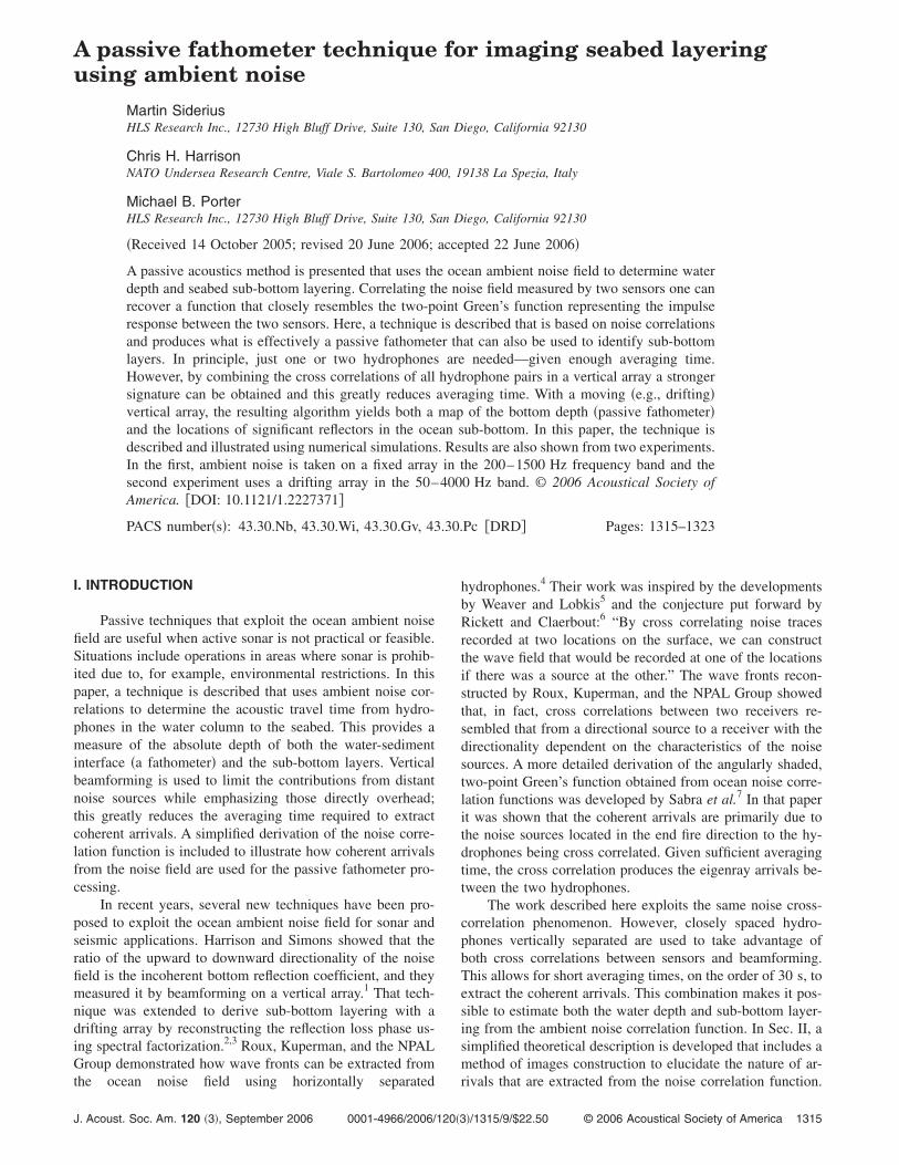
that the bottom bounce is similar to the case of the perfectlyreflecting boundary with the exception of the higher loss onthe bottom bounce. One of the differences with this simula-tion occurs near time lag zero. A zoomed in display in panel�b� shows a wave front arriving more horizontally than thebottom bounce �the M-shape near time zero�. The angle ofthis wave front corresponds to the critical angle of the1550 m/s seabed. To compare, in panel �c� the seabed soundspeed is changed to 1750 m/s and the angle of the wavefront has increased. These wave fronts that occur at the criti-cal angle suggest this process is detecting the head wave.These wave fronts, near time-lag zero, are at angles that aredifferent from the bottom bounce and will have insignificantimpact on the passive fathometer processing. They may,
FIG. 6. In panel �a� a realistic �lossy� seabed is used with the same geometryas for panel �b� of Fig. 5. Note, the wavefronts near time-lag zero arepropagating at a more horizontal angle relative to the bottom bounce �theM-shape near time zero�. In panel �b� is a zoom of �a� showing the details ofthe wavefront. The propagation angle of the wavefront in �b� corresponds tothe critical angle of the seabed. In �c� the seabed sound speed is changed to1750 m/s and the steeper propagation angle of the wavefront near time-lagzero can be seen.
J. Acoust. Soc. Am., Vol. 120, No. 3, September 2006
however, be important for identifying the critical angle of theseabed if they can also be detected using measured data.They will not be considered further in this paper as the focusis on the bottom and sub-bottom returns.
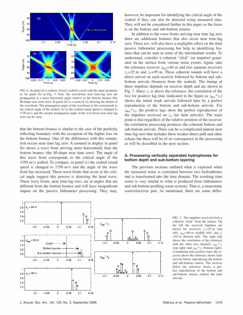
In addition to the wave fronts arriving near time lag zerothere are additional features that also occur near time-lagzero. These too, will also have a negligible effect on the finalpassive fathometer processing but help in identifying fea-tures that can be seen in some of the intermediate results. Tounderstand, consider a coherent “click” �or impulse� gener-ated on the surface from various noise events. Again, takethe reference receiver zRef=60 m and two separate receiversz1=25 m and z2=95 m. These coherent sounds will have adirect arrival on each receiver followed by bottom and sub-bottom arrivals �bounces from the seabed�. The timing ofthese impulses depends on receiver depth and are shown inFig. 7. Since z1 is above the reference, the correlation of thetwo for positive lag time �indicated in the figure as zRef*z1�shows the initial weak arrivals followed later by a perfectreproduction of the bottom and sub-bottom arrivals. ForzRef*z2, the positive lags show the perfect reproduction ofthe impulses received on z2 �no faint arrivals�. The mainpoint is that regardless of the relative position of the receiver,the correlation processing produces the coherent bottom andsub-bottom arrivals. There can be a complicated pattern neartime-lag zero that includes these weaker direct path and otherechoes but these will be of no consequence in the processingas will be described in the next section.
A. Processing vertically separated hydrophones forbottom depth and sub-bottom layering
The previous sections outlined what is expected whenthe measured noise is correlated between two hydrophonesand is transformed into the time domain. The resulting timeseries is very similar to what is produced from fathometersand sub-bottom profiling sonar systems. That is, a monostaticsource/receiver pair. As mentioned, there are some differ-
FIG. 7. The impulses received from acoherent “click” from the surface. Onthe left the received impulses areshown for receivers z1=25 m �topleft�, zRef=60 m �middle left�, and z2
=95 m �bottom left�. The right sideshows the correlation of the referencewith the other two channels, zRef*z1
�top right� and zRef*z2 �bottom right�.Considering only positive time, the re-ceiver above the reference shows faintarrivals before reproducing the bottomand sub-bottom returns. The receiverbelow the reference shows a per-fect reproduction of the bottom andsub-bottom returns without the faintarrivals.
Siderius et al.: Passive fathometer 1319
ences between a true source/receiver and the noise correla-tion processing. The noise correlation processing produces atime series with some directionality and there are arrivalsbefore time-lag zero. Another difference includes arrivalsnear time-lag zero due to a variety of effects as describedpreviously. However none of these have a significant impacton the ambient noise fathometer/sub-bottom profiler. Theonly caveat is that the time-series synthesis must be longenough to prevent wrap around. The time series length is setby the selected frequency sampling in the cross-spectral den-sity and, in practice, can be set arbitrarily small.
Next, consider a more realistic simulation consisting of alayered seabed and a realistic array which will be used forthe beam-forming part of the processing. The array has thesame characteristics as one that is used for the measured dataanalysis in Sec. IV and has 32 vertically separated hydro-phones located between depths of 70 to 75.58 m �0.18 mspacing�. The seabed is made up of a top 10 m layer withsound speed of 1550 m/s, density of 1.5 g/cm3, and attenu-ation of 0.06 dB/�. Below that is a 5 m layer with soundspeed of 1600 m/s, density of 1.65 g/cm3, and attenuationof 0.2 dB/�. The half-space below both sediment layers hassound speed of 1700 m/s, density of 1.65 g/cm3, and attenu-ation of 0.2 dB/�. To simulate the noise field, Eq. �1� isevaluated using the OASES program.12,15
The first fathometer processing step is to correlate eachreceiver in the array with each of the others to form thecross-spectral density at all frequencies �in this simulationfrequencies between 50 and 4000 Hz are included�. The timeseries is derived from the frequency domain correlation be-tween receivers at zn and zm using Eq. �14�. The bottombounce absolute travel times will correspond to the traveltime from the reference receiver to the seabed plus the traveltime back to each of the other receivers in the array. Regard-less of the receiver chosen as the reference the bottombounce arrivals will appear delayed from the bottom of thearray to the top. These arrivals can all be combined by ap-plying the correct time delay to align the receptions. Thealignment is accomplished through delay and sum beam-forming �in the end-fire direction�
C̃n��� =1
M�m=0
M−1
C�� + m�,zn,zm� , �15�
where
� =zh
cw. �16�
The time delay between receivers is � and zh is the re-ceiver separation and cw is the water sound speed.
With receiver 1 �shallowest at 70 m� as the reference,the first bottom reflection arrives on channel 32 �at depth75.58 m� at time
�100 − 70� + �100 − 75.58�1500
= 0.0363 s, �17�
and arrives at channel 1 at 0.04 s. The 32 channels arecombined with the appropriate delay to form a single time
trace. Next, channel 2 is used as the reference and the 32
1320 J. Acoust. Soc. Am., Vol. 120, No. 3, September 2006
receivers are beamformed again. Since channel 2 is thereference, the bottom bounce arrivals arrive earlier by ��since the effective source is now closer to the seabed�.The process is repeated until 32 time traces are formed.This first stage of beamforming produces an arrival struc-ture for each reference hydrophone n=1¯32 and is illus-trated in panel �a� of Fig. 8. In panel �a� each row is theresult using a different reference channel which causes thedelayed arrivals from the seabed. The bottom and sub-bottom reflections are visible with travel times relative n=1 �receiver at 70 m depth� since all beamforming is donerelative to this receiver.
The time series shown in panel �a� of Fig. 8 is combinedagain using delay and sum beamforming. This final stepaligns the bottom and sub-bottom arrivals into a single timeseries r���
r��� =1
N�n=0
N−1
C̃n�� + n�� . �18�
This is shown in panel �b� of Fig. 8 where the bottom andsub-bottom returns are clearly visible. The absolute waterdepth can be determined from the two-way travel times takenfrom depth of receiver n=1. In this case the first arrival is at0.04 s corresponding to �30�2� /1500 s. The sub-bottomlayers are also two-way travel times relative to the previ-ous bottom reflection. The next arrival occurs after anadditional �10�2� /1550 s, or at 0.0529 s. The final arrivalis later by and additional �5�2� /1600 s, or at 0.0592 s.There are residual peaks near the zero lag of the timeseries that can be ignored in the processing since thesepeaks are predictable from the length of the array. In thiscase the peaks occur between time zero and time 0.0074 s�twice the travel time of the length of the array due to the
FIG. 8. Panel �a�: Stacked, delay, and sum beamforming �i.e., C̃n�t� withn=1¯32�. Note, there is a bottom reflection corresponding to the water-seabed interface and two sub-bottom reflections corresponding to the twolayers. Time series magnitudes are shown on a decibel scale with a range of30 dB. Panel �b�: the second stage of beamforming �i.e., beamforming thesequences shown in panel �a� and given by the expression for r�t��. This ison a normalized linear scale where the envelope has been taken.
two stages of beamforming�.
Siderius et al.: Passive fathometer
In these simulations, the cross-spectral density that wascalculated is idealized and assumes an infinite averagingtime. Long averaging is probably not practical for applica-tion as a survey tool since the integration times would needto be relatively short. The beamforming greatly assists theshortened averaging time with measured data by emphasiz-ing the coherent part of the noise field coming from directlyover the vertical array. As will be seen with the experimentaldata in the next section, with short averaging times the beam-forming is critical to observing the bottom arrivals.
IV. EXPERIMENTAL RESULTS
Two measured data examples of the fathometer process-ing will be presented. The first example uses measured dataof opportunity. The experiment had an active source �10 kmfrom the receiver array� so the ambient noise was carefullywindowed from the time series. This experiment had a fixedarray with carefully measured array and water depths so itverifies the processing in a known environment. The secondexample is taken from a more practical scenario with thevertical array drifting over a varying bathymetry and sub-bottom. These arrays are both electronically quiet havingelectronic noise floor below sea-state zero.
A. Stellwagen Bank: ASCOT01
In 2001, the NATO Undersea Research Centre con-ducted the ASCOT-01 experiment near the Stellwagen Bankoff the Northeast coast of the United States in a site with101 m water depth.16 This was primarily a geo-acoustic in-version experiment so sound sources were nearly continu-ously transmitting with the exception of about 0.5 s of dataat the end of each file. Since the vertical array was fixed,these 0.5 s snapshots could be averaged over many snapshotsproducing, effectively, about a 30 s average. The soundsource was located 10 km away and the ambient noise datawas believed to be free from multipath and reverberationfrom the projector. The fixed and well measured geometry ofASCOT-01 provides a useful check of the bottom return tim-ing.
A total of 33 elements with 0.5-m spacing array wereused with the top hydrophone measured to be 52.25 m fromthe seabed. The frequency band considered is 200–1500 Hz.In Fig. 9, panel �a� shows the output after the first stage ofbeamforming. The bottom bounce is weak yet visible. Fromthe single-phone correlations, the bottom returns were tooweak to be visible without beamforming. In panel �b� of Fig.9, the second stage of beamforming is applied and the bot-tom bounce is clearly visible. The peak near 0.07 s, in panel�b� puts the estimate of the distance to the bottom at 52.5 m,well within the experimental error on the measured hydro-phone distance of 52.25 m. In this case, the array referencewas the shallowest channel at 52.25 m which is near themidwater depth, and if a surface bounce were present, itwould nearly interfere. To break the symmetry, the arraybeamforming was shifted to the deepest hydrophone and thisis shown in panel �c� of Fig. 9. As predicted, in neither caseis there evidence of a surface bounce. This may primarily be
due to the beamforming deemphasize this return, but was
J. Acoust. Soc. Am., Vol. 120, No. 3, September 2006
also seen to be weaker than might be expected from a truesource as discussed previously. Sub-bottom returns are alsopresent, but these could not be verified for correctness.
B. Strait of Sicily: Boundary 2003
The second experimental example is taken from a con-trolled set of �directional noise� data that were collected �bythe second author� on a drifting array during the NATO Un-dersea Research Centres Boundary 2003 experiment. �This isthe same data set as described in Ref. 3 where it was con-verted to sub-bottom layers by a different process.� The drift-ing array has 32 hydrophones spaced at 0.18 m �design fre-quency of 4.2 kHz�. The wind varied during the experimentbut was, on average, approximately 15 kn. The array was notequipped with a Global Positioning System receiver but wastracked using surface radar. At the time of the experiment,the depth of the array was not a critical factor and was there-fore not measured carefully. However, it was reported that
FIG. 9. Panel �a� shows the ASCOT-01 ambient noise processing after thefirst stage of beamforming. Near time zero, the direct arrival is visible ar-riving at later times as the wave front progresses down the array. In panel �b�is the second stage of beamforming showing the bottom bounce at around0.07 s. Panel �c� shows the same processing with the array center shifted tothe deepest hydrophone.
the hydrophones were to be kept less than about 80 m but
Siderius et al.: Passive fathometer 1321
were probably between 70 and 80 m. The signals weresampled at 12 kHz and each channel was transformed to thefrequency domain using 16384 point fast Fourier transforms�FFTs� �or around 1.4 s of data�. Approximately 70 s of datawere averaged to form the cross-spectral density and producea single fathometer time trace �over the 50–4000 Hz fre-quency band�.
Following the array drift, seismic reflection data werecollected to image the sub-bottom layers. The seismic reflec-tion data was collected by towing a Uniboom source �5813Bseismic boomer� with a ten element towed array behind theNATO R /V Alliance. This sonar is designed to measure boththe bathymetry and the strongest reflectors from the seabed.It was only possible to approximate the drifting array trackswith the Uniboom tracks.
In Fig. 10, the ambient noise �panel �a�� and Uniboom�panel �b�� processed data are shown. For these displays. thedata envelope of the time series are taken and put on a deci-bel scale. There is a 12 dB dynamic range in the color scale.
FIG. 10. In panel �a� the ambient noise fathometer processing is used and inpanel �b� approximately the same track using a towed Uniboom sub-bottomprofiler. The y axis is two-way travel times converted to depths using1500 m/s sound speed.
Since the array depth and position were not known exactly,
1322 J. Acoust. Soc. Am., Vol. 120, No. 3, September 2006
some alignment of the ambient noise and Uniboom data weremade with the data itself. The depth of the array was taken as73.5 m for the entire track. The range of the array along thetrack was allowed to slide a few hundred meters. However, asingle range correction was used for the entire track. Thereare features in both �a� and �b� that are similar as far down as25 m into the seabed. The map of the bathymetry from thenoise �panel �a�� also closely resembles that from the Uni-boom survey.
V. SUMMARY AND CONCLUSIONS
Using the coherent components of the ocean ambientnoise, a passive fathometer and seabed layer imaging tech-nique has been described. In theory, this might be done witha single receiver, however this may require averaging timestoo long to be practical. Using a vertical array of receivers,beamforming on enfire was used to emphasize the coherentarrivals coming from directly above the array. Beamformingallows averaging the noise over a short time which then re-sembles random clicks coming from the surface. The pro-cessing technique has been illustrated with simulations, how-ever, these simulations assumed infinite averaging time.Experimental data shows the processing also works with rea-sonable averaging times of about one minute. The first ex-ample showed a fixed array with carefully measured geom-etry and the bottom bounce path arriving at exactly thepredicted time. The second example used a drifting array thatshowed both bathymetry and sub-bottom layering. A sub-bottom profiling sonar was taken along the same path as thedrift to validate the results from the passive fathometer pro-cessing.
ACKNOWLEDGMENTS
This research was sponsored by the Office of Naval Re-search Ocean Acoustics Program. Additional support wasprovided by the Office of Naval Research PLUSNet Pro-gram.The authors would like to thank the NATO UnderseaResearch Centre for the experimental data support. In par-ticular, Jurgen Sellschopp and Peter Nielsen for the AS-COT01 experiment and to Peter Nielsen for the Boundary2003 experiment. Thanks also to Paul Hursky for many valu-able discussions.
1C. H. Harrison and D. G. Simons, “Geoacoustic inversion of ambientnoise: A simple method,” J. Acoust. Soc. Am. 112�4�, 1377–1389 �2002�.
2C. Harrison, “Sub-bottom profiling using ocean ambient noise,” J. Acoust.Soc. Am. 115�4�, 1505–1515 �2004�.
3C. Harrison, “Performance and limitations of spectral factorization forambient noise sub-bottom profiling,” J. Acoust. Soc. Am. 118�5�, 2913–2923 �2005�.
4P. Roux, W. A. Kuperman and the NPAL Group, “Extracting coherentwave fronts from acoustic ambient noise in the ocean,” J. Acoust. Soc.Am. 116�4�, 1195–2003 �2004�.
5R. L. Weaver and O. I. Lobkis, “Ultrasonics without a source: Thermalfluctuation correlations at MHz frequencies,” Phys. Rev. Lett. 87, 134301�2001�.
6J. Rickett and J. Claerbout, “Acoustic daylight imaging via spectral fac-torization: Helioseismology and reservoir monitoring,” Report 100, Stan-ford Exploration Project �unpublished�.
7K. G. Sabra, P. Roux, and W. A. Kuperman, “Arrival-time structure of thetime-averaged ambient noise cross-correlation function in an oceanic
waveguide,” J. Acoust. Soc. Am. 117�1�, 164–174 �2005�.
Siderius et al.: Passive fathometer
8M. J. Buckingham, “A theoretical model of ambient noise in a low-lossshallow water channel,” J. Acoust. Soc. Am. 67�4�, 1186–1192 �1980�.
9C. H. Harrison, “Formulas for ambient noise level and coherence,” J.Acoust. Soc. Am. 99�4�, 2055–2066 �1996�.
10W. A. Kuperman and F. Ingenito, “Spatial correlation of surface generatednoise in a stratified ocean,” J. Acoust. Soc. Am. 67�6�, 1988–1996 �1980�.
11F. B. Jensen, W. A. Kuperman, M. B. Porter, and H. Schmidt, Computa-tional Ocean Acoustics �American Institute of Physics, Inc., New York,1994�.
12H. Schmidt, “SAFARI: Seismo-acoustic fast field algorithm for range in-dependent environments. User’s guide,” SR-113, SACLANT Undersea
Research Centre, La Spezia, Italy �unpublished�.
J. Acoust. Soc. Am., Vol. 120, No. 3, September 2006
13H. Schmidt and F. B. Jensen, “A full wave solution for propagation inmultilayered viscoelastic media with application to Gaussian beam reflec-tion at fluid-solid interfaces,” J. Acoust. Soc. Am. 77, 813–825 �1985�.
14B. F. Cron and C. H. Sherman, “Spatial-correlation functions for variousnoise models,” J. Acoust. Soc. Am. 34, 1732–1736 �1962�.
15H. Schmidt, “OASES version 3.1 user guide and reference manual,” http://acoustics.mit.edu/faculty/henrik/oases.html, Department of Ocean Engi-neering Massachusetts Institute of Technology, Cambridge, MA �unpub-lished�.
16J. Sellschopp, NATO Undersea Research Centre, Vaile S. Barolomeo 400,19138 La Spezia, Italy, ASCOT-01, SACLANTCEN CD-ROM, 49, 2001.