Page 1
A Performance EvaluationArchitecture for PNNI
Sandeep Bhat, Doug Niehaus, Victor Frost
ITTC-FY99-TR-13200-07
Februaryr1999
Copyright © 1999:The University of Kansas Center for Research, Inc.,2291 Irving Hill Road, Lawrence, KS 66044-7541;and Sprint Corporation.All rights reserved.
Project Sponsor:Sprint Corporation
Technical Report
The University of Kansas
Page 2
Abstract
As larger ATM networks are being installed, the performance issues relating to Pri-vate Network to Network Interface(PNNI) protocol, which provides link state baseddynamic routing capability in an ATM network have assumed significance. The fac-tors influencing the selection of topology of a network, the number of nodes in thenetwork which share topology information(Peer Group size), the call setup times, linkutilization, call rejection rates need to be evaluated. A comprehensive simulation toolfor evaluating PNNI protocol is developed. The simulation tool is developed on a soft-ware architecture which has all the modules which are required to control an ATMswitch, enabling its simulations closer to real network characteristics. Connection re-quests are generated using a comprehensive call generating tool. The factors influenc-ing the peer group size and performance of a single peer group PNNI are addressedtaking the topology convergence times, call setup times, bandwidth requirement of thePNNI topology messages, topology messages per call, source node failed calls, inter-mediate node failed calls and route computation times as metrics. The performance ofthe simulator to run sensible simulations is addressed.
Page 3
Contents
1 Introduction 1
2 Related Work 7
2.1 ATM Connection Setup Sequence . . . . . . . . . . . . . . . . . . . . . . . 7
2.2 PNNI Features . . . . . . . . . . . . . . . . . . . . . . . . . . . . . . . . . . 8
2.3 PNNI Topology . . . . . . . . . . . . . . . . . . . . . . . . . . . . . . . . . 9
2.4 PNNI Routing . . . . . . . . . . . . . . . . . . . . . . . . . . . . . . . . . . 12
2.5 PNNI Metrics and Attributes . . . . . . . . . . . . . . . . . . . . . . . . . 13
2.6 PNNI Signaling . . . . . . . . . . . . . . . . . . . . . . . . . . . . . . . . . 14
2.6.1 Designated Transit Lists . . . . . . . . . . . . . . . . . . . . . . . . 14
2.6.2 Crankback and Alternate Routing . . . . . . . . . . . . . . . . . . 15
2.7 Performance Measurement Tools for PNNI . . . . . . . . . . . . . . . . . 16
3 Implementation 18
3.1 Simulation Model . . . . . . . . . . . . . . . . . . . . . . . . . . . . . . . . 18
3.1.1 Simulation Kernel . . . . . . . . . . . . . . . . . . . . . . . . . . . 20
3.1.2 Priority of Servicing . . . . . . . . . . . . . . . . . . . . . . . . . . 21
3.1.3 Simulation of Link and Queueing Delays . . . . . . . . . . . . . . 21
3.1.3.1 Simulation of Links Between Ports . . . . . . . . . . . . 22
3.1.3.2 LinkDelays and Queuing delays . . . . . . . . . . . . . . 23
3.2 Q93B PNNI Stack and DTL Processing . . . . . . . . . . . . . . . . . . . . 23
3.3 Switch Call Control Support for PNNI . . . . . . . . . . . . . . . . . . . . 26
3.4 PNNI Routing Services (PNNI RS) . . . . . . . . . . . . . . . . . . . . . . 27
i
Page 4
3.4.1 Interaction between PNNI RS and SCC . . . . . . . . . . . . . . . 27
3.4.2 Interaction Between the PNNI RS and the AAL5 module . . . . . 29
3.4.3 PNNI Routing Module’s Functionalities . . . . . . . . . . . . . . . 32
3.5 Results and Logging Format . . . . . . . . . . . . . . . . . . . . . . . . . 34
3.6 User Input Interface . . . . . . . . . . . . . . . . . . . . . . . . . . . . . . . 36
3.7 Call Generator Changes . . . . . . . . . . . . . . . . . . . . . . . . . . . . 36
4 Evaluation 40
4.1 Experiments With Abstract Topologies . . . . . . . . . . . . . . . . . . . . 40
4.1.1 Topology Convergence Time . . . . . . . . . . . . . . . . . . . . . 41
4.1.1.1 Convergence Time With Increasing Number of Nodes . 42
4.1.1.2 Differing Convergence Times Among Nodes . . . . . . 43
4.1.1.3 Convergence Time With Varying Connectivity Density . 44
4.1.1.4 Convergence Time With Varying Processing Delays . . 44
4.1.1.5 Convergence Time with Varying Link Delays . . . . . . 46
4.1.2 Topology Updates With Different Network Topologies . . . . . . 46
4.2 Experiments With Realistic Topologies . . . . . . . . . . . . . . . . . . . . 48
4.2.1 Topology description . . . . . . . . . . . . . . . . . . . . . . . . . . 48
4.3 Call Generation Experiments Related To Proportional Multiplier . . . . . 51
4.3.1 PNNI Topology Update Messages . . . . . . . . . . . . . . . . . . 52
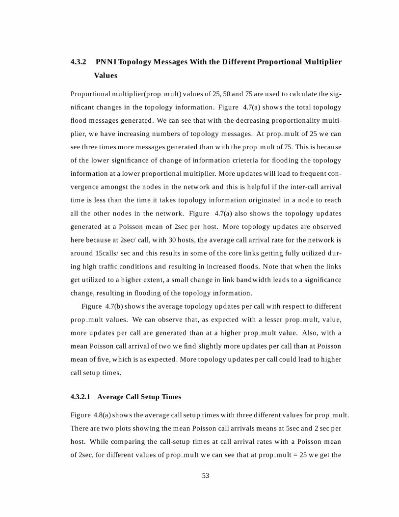
4.3.2 PNNI Topology Messages With the Different Proportional Mul-
tiplier Values . . . . . . . . . . . . . . . . . . . . . . . . . . . . . . 53
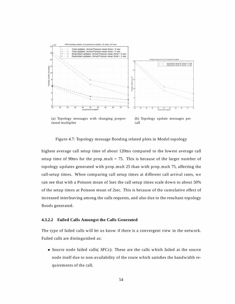
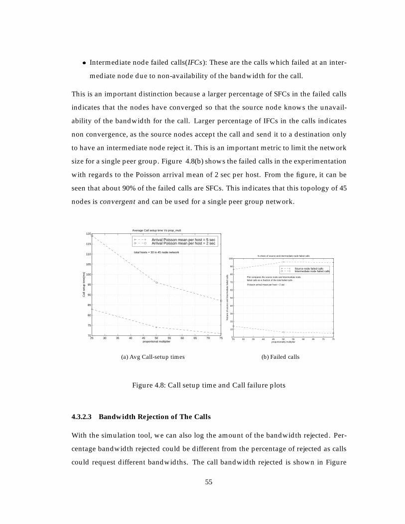
4.3.2.1 Average Call Setup Times . . . . . . . . . . . . . . . . . . 53
4.3.2.2 Failed Calls Amongst the Calls Generated . . . . . . . . 54
4.3.2.3 Bandwidth Rejection of The Calls . . . . . . . . . . . . . 55
4.4 Improvement In Percent Call Success Rate . . . . . . . . . . . . . . . . . . 56
4.5 Routing with Different Routing Policies . . . . . . . . . . . . . . . . . . . 57
4.6 The Performance of the PNNI Protocol with Expanding Networks . . . . 59
4.7 Performance of Simulator . . . . . . . . . . . . . . . . . . . . . . . . . . . 61
ii
Page 5
5 Conclusions and Future Work 62
5.1 Future Work . . . . . . . . . . . . . . . . . . . . . . . . . . . . . . . . . . . 63
iii
Page 6
List of Tables
3.1 Designated transition List . . . . . . . . . . . . . . . . . . . . . . . . . . . 25
4.1 Link bandwidths for different links . . . . . . . . . . . . . . . . . . . . . . 49
4.2 Call sources and QoS requirements . . . . . . . . . . . . . . . . . . . . . . 51
iv
Page 7
List of Figures
2.1 ATM Connection Setup Message Sequence . . . . . . . . . . . . . . . . . 7
2.2 PNNI hierarchical architecture . . . . . . . . . . . . . . . . . . . . . . . . 10
3.1 PNNI Simulator Model . . . . . . . . . . . . . . . . . . . . . . . . . . . . . 19
3.2 Q.93B port stack . . . . . . . . . . . . . . . . . . . . . . . . . . . . . . . . . 22
3.3 Interaction between SCC and PNNI RS Modules . . . . . . . . . . . . . . 27
3.4 Hello and Node Peer FSMs . . . . . . . . . . . . . . . . . . . . . . . . . . 30
3.5 Messaging between PNNI RS and AAL5 . . . . . . . . . . . . . . . . . . 31
3.6 Logging mechanism for results . . . . . . . . . . . . . . . . . . . . . . . . 34
3.7 Design of common interface to simulator and emulator . . . . . . . . . . 37
4.1 Chain, Ring and Mesh topologies . . . . . . . . . . . . . . . . . . . . . . . 41
4.2 Topology Convergence time related plots . . . . . . . . . . . . . . . . . . 42
4.3 Topology Convergence time related plots . . . . . . . . . . . . . . . . . . 45
4.4 Topology message flooding related plots . . . . . . . . . . . . . . . . . . . 47
4.5 Edge core topology of 45 nodes . . . . . . . . . . . . . . . . . . . . . . . . 50
4.6 Topology update messages . . . . . . . . . . . . . . . . . . . . . . . . . . 52
4.7 Topology message flooding related plots in Model topology . . . . . . . 54
4.8 Call setup time and Call failure plots . . . . . . . . . . . . . . . . . . . . . 55
4.9 Call Rejection and Bandwidth Rejection Plots . . . . . . . . . . . . . . . . 56
4.10 Utilization and Call success improvement . . . . . . . . . . . . . . . . . . 57
4.11 Call Success with different routing policies . . . . . . . . . . . . . . . . . 58
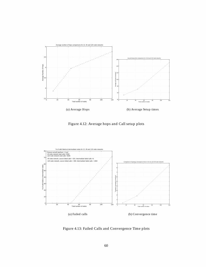
4.12 Average hops and Call setup plots . . . . . . . . . . . . . . . . . . . . . . 60
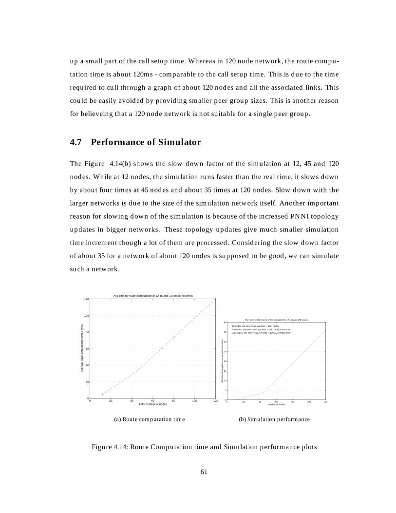
4.13 Failed Calls and Convergence Time plots . . . . . . . . . . . . . . . . . . 60
v
Page 8
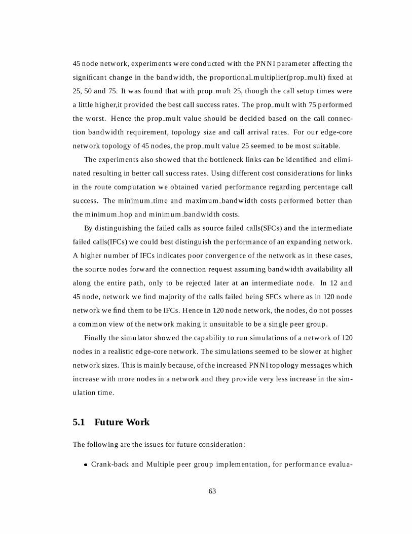
4.14 Route Computation time and Simulation performance plots . . . . . . . 61
vi
Page 9
List of Programs
3.1 Simulation Kernel Service Routine . . . . . . . . . . . . . . . . . . . . . . 21
3.2 Pass thru link between ports . . . . . . . . . . . . . . . . . . . . . . . . . . 23
3.3 Queueing and Link Delays . . . . . . . . . . . . . . . . . . . . . . . . . . . 24
3.4 The host call record . . . . . . . . . . . . . . . . . . . . . . . . . . . . . . . 35
3.5 The node call record . . . . . . . . . . . . . . . . . . . . . . . . . . . . . . 36
vii
Page 10
Chapter 1
Introduction
The Private Network to Network protocol(PNNI) is a comprehensive routing and sig-
naling protocol architecture in a private Asynchronous Transfer Mode Network(ATM).
It helps in exchanging the routing related topology information between ATM nodes.
It also helps in selecting a source route to the destination when a call connection is
requested. PNNI uses the topology database it developed through flooding, to gener-
ate a source route to the destination required. The PNNI protocol is a very complex
protocol to implement and it is even more difficult to predict its performance. The
network behavior becomes unpredictable when controlling a big private network of
ATM nodes(also known as switches), because connection requests will be coming from
different host systems in the network, in unknown arrival patterns, with unexpected
bandwidth requirements, and with different call connection durations. The PNNI pro-
tocol also contributes to this unpredictability by offering a wide range of parameters
that may be manipulated.
One of the important issues of PNNI performance is its scalability. The PNNI proto-
col receives knowledge of the changing network through topology updates generated
whenever there is a significant change in the topology information. These topology
messages are broadcast to all the nodes in a network. In an expanding network, the
link delays, the flooding delays due to redundancy, and the node processing delays
impose a considerable delay before the information reaches all the intended network
nodes. This could cause wrongly rejected calls due to false belief in lack of band-
1
Page 11
width in the network as well as wrongly accepted calls which will only be rejected later.
Hence when the network service providers invest in installing an expensive ATM net-
work, they seek to know about the performance of their network. Before deployment,
it is of paramount importance to design a network for future extendibility. Testing a
network’s performance is a complex evaluation process as it is dependent on a number
of parameters. To list some of them:
� the network topology.
� the connectivity density between the nodes.
� link bandwidth and link delays.
� call arrival rates.
� the call bandwidth requirements.
� the parameters of the PNNI protocol involved such as the flooding significance
and the minimum threshold parameters for the topology information flooding.
� the switch port packet queue size and related packet losses,
� the difference in the relative processing capabilities of the nodes,
� the different routing policies that are used.
The list could be longer. This produces an unbounded problem which is beyond the
reach of any mathematical solution. But nevertheless it is essential to have some type
of performance prediction system, which could enable us to study the performance of
the network.
The options to test the performance could be that the network providers have a
test network of ATM nodes for testing purposes alone. But though such networks ex-
ist, they are only used for advanced network testing such as interoperability testing
between two switch vendor’s switches and a few basic sanity tests, and not for wide
ranging performance evaluation test suites. Such test networks are also relatively small
compared to an actual deployed network. These networks cannot be used for wide
2
Page 12
ranging performance tests because the setting up of such networks for the required
experimentation is very time consuming, difficult, very expensive, and multiple such
networks for simultaneous performance experimentation is not affordable. Succinctly,
using real networks for all tests is not feasible, and since a great deal of effort is in-
volved to get simplest of performance measures, this approach is not worthwhile.
The best alternative we find in such cases is either to simulate such networks or
to emulate them in a distributed environment. While emulations scale to very large
networks, simulations are very efficient for medium to large scale networks. While
emulation is under advanced stages of development, simulation is used in this thesis
for performance evaluation. Simulation is a software process which runs on a single
workstation. It is configurable to simulate a required network with various network
entities. It is also possible to specify the collection of various performance related data
at different times during the experimentation. The simulations and emulations save
time by offering simultaneous experimentation and are economically feasible.
The simulation is supported on the Bellcore’s Q.port software. This software in-
cludes the UNI signaling messages, the data link Qsaal layer. GSMP off-board signal-
ing agent capability is also added in the software which can control an ATM switch.
Emulation support is also added to Q.port. The simulation model is built on this soft-
ware with all necessary protocol stacks in the real ATM switch being used in the sim-
ulation to make it more real and accurate. The off-board signaling agent fabric, the
emulation fabric, and the simulation model have about 98 % of their software in com-
mon.
The motivation to evaluate the performance of the PNNI protocol has led to devel-
oping a PNNI simulator as described in this thesis. The initiative to develop a simu-
lator was taken up as there were no simulator tools available for PNNI performance
testing which we required. At the time of developing this thesis, it was decided to use
Naval Research Laboratory’s(NRL) Proust simulator, but the Proust simulator did not
support the call generation capabilities and it was primitive in some respects. Nortel
(Northern Telecom) is working on a simulation tool which is in a development stage
and not much is known about its capabilities. So simulator development was taken up
3
Page 13
which could help us test the performance of PNNI and extend our experimentation by
expanding the tool’s capability in a future perspective.
The simulator supports a single peer group version of the ATM forum PNNI spec-
ification. It is designed to an architecture which is convenient to be used, and which
supports configuring and monitoring all the possible PNNI parameters of interest for
experimentation. The Q.port software from Bellcore is used for the purpose of de-
veloping the simulator. Q.port’s real time scheduling system is modified to support
the virtual time oriented simulations. The Q.port software is upgraded to support an
additional PNNI element, the Designated Transition List(DTL). The DTL contains the
source node generated list of nodal hops to be traversed to reach the destination of the
requested call. NRL’s Proust PNNI architecture is interfaced in Q.port for providing
the PNNI routing subsystem module. The most important finite state machine (FSM)
in the PNNI protocol, the Node Peer FSM (NPFSM), the associated topology database
interface, the decoding and encoding of the topology messages are developed for NRL
by us which is reciprocated by the NRL in letting us use its software for the simulator.
The NPFSM exchanges the topology information between the nodes and helps keep a
database of all the topology information in each node. It interacts with the database
to either seek topology information for broadcasting to other nodes or to insert new
topology elements, it obtained from other nodes.
The simulator provides convenient usage of the tool by supporting a user input
script language, which specifies
� The duration of the simulation.
� The network size in terms of the total number of nodes and links. Generic node
characteristics and the individual node characteristics. Node characteristics in-
clude the routing policies, the PNNI protocol timer values, the proportional mul-
tiplier and minimum threshold values for effecting the significance of topology
information change which leads to its flooding, and the number of ports.
� The connectivity between nodes, link bandwidth, queue size, link delays, and
queuing delays.
4
Page 14
� The generic and individual host characteristics, the different call arrival and du-
ration distributions, prominently, uniform, Poisson, and periodic distributions.
Multiple traffic sources with different destinations, bandwidth requirements, QoS
requirements, and total number of calls to be attempted.
The user input script is designed in a manner to help users specify the minimum re-
quired parameters to run an experiment.
The tool supports the instrumentation of the following performance evaluation pa-
rameters:
� Link utilization.
� Call setup times.
� Initial PNNI topology convergence time.
� Call failure causes.
� The number of PNNI topology messages sent.
� The bandwidth consumed by PNNI messages.
� Call failures at the source node itself due to the knowledge of unavailability of
network bandwidth.
� Call failures due to non availability of bandwidth in an intermediate link.
� Average hop length for each calls.
� Routing algorithm computation time.
The rest of this report is structured in the following manner. Chapter 2 explains the
features of the PNNI protocol whose performance is studied under this thesis. Chapter
3 discusses the implementation aspects involved in the simulator. Chapter 4 explains
the PNNI single peer group experiments conducted and the analysis of the perfor-
mance obtained. The performance of the simulation tool regarding bigger network
simulation is also discussed. Chapter 5 details the conclusions from the results and
5
Page 15
things learned from the thesis. It also explains the future enhanment of the simulator
capabilities, providing the multiple peer group support and the specific performance
issues of interest.
6
Page 16
Chapter 2
Related Work
The Private Network to Network Interface protocol(PNNI) provides a scalable, dy-
namic routing architecture to support the ATM connection setup requests. In this
chapter the basic ATM signaling connection setup sequences will be explained first.
This will be followed with explanations on PNNI’s specific features, hierarchical archi-
tecture, routing, and signaling information elements. Finally, the currently available
research and commercial tools which support PNNI signaling will be presented.
2.1 ATM Connection Setup Sequence
SWITCH
SETUP
CALL_PROCEEDINGSETUP
CONNECT
CONNECT_ACKCONNECT
CONNECT_ACK
AND DATA TRANSFERCONNECTION UP
CALLING HOST CALLED HOST
Figure 2.1: ATM Connection Setup Message Sequence
The flow of the ATM signaling sequences is illustrated in Figure 2.1. The calling
7
Page 17
host sends the setup message to the switch requesting a connection to the called host.
The switch finds the route to the called host and forwards the setup message to the
selected port connected to the called host. The called host receives the setup message
and on deciding to accept the connection, sends the connect message to the switch.
The switch receives the connect message and sends the connect ack message to the
destination host which accepts it and prepares for data transfer. The switch sends a
connect message to the calling host. The calling host receives the connect message
and sends the connect ack message to the switch which accepts it. The connection is
established. The calling and the called hosts exchange data.
2.2 PNNI Features
It is envisioned that ATM will grow and evolve into large networks consisting of a large
number of switches connected by high-speed links. Many thousands of (Switched
Virtual Circuit) SVC requests will be submitted to the network and the network will be
expected to forward each request to the right destination, establish a path from calling
to the called host, allocate resources and guarantee QoS. It will be a challenging task
selecting the right path, one that optimizes network resources and guarantees QoS. The
network itself may be made up of a mixture of ATM switches from different vendors.
Different switches could set their own policies and procedures in the switch. PNNI is
designed to support these challenging needs of a dynamic ATM network. Its features
include:
� Scalability: It supports both small and very large networks of ATM switches.
� Simple to install and configure: As soon as the switches are connected, they ex-
change topology information and are able to route SVC requests with minimal
configuration.
� Dynamic routing mechanism: PNNI supports dynamic routing of SVC requests
through the network. In larger networks PNNI provides scalable hierarchical
routing and support for multiple routing metrics and attributes. The best path
8
Page 18
that will meet QoS objectives in the SVC request is computed and then the SVC
request forwarded along that path. The routing is also responsive to changes in
resource availability.
� Source or transit policies support: PNNI enables both source or transit policies
to be administered. Different switch domains may have different policies based
on security, usage, traffic types and other vendor specific issues.
� Multi vendor: PNNI supports a network of multi vendor switches and allows in-
teroperability between them. The individual switches of different vendors could
perform some specific functions such as route computation and Connection Ad-
mission Control(CAC) and others which suit their policy.
� Interoperability : PNNI supports interoperability with external routing domains,
like Internet Protocol(IP) and others, not necessarily using PNNI. In Integrated
PNNI the ATM switches exchange topology information with the IP routers to
maintain routing database.
2.3 PNNI Topology
PNNI topology constitutes the PNNI routing hierarchy. These are terms associated
with a PNNI topology. Please refer to Figure 2.2 along with explanation of the terms
when required.
� Peer Group (PG): A peer group is a collection of nodes that shares the topol-
ogy information generated by each node through topology information flooding.
Members of a peer group discover their neighbors using a hello protocol. Phys-
ical peer groups consist of physical nodes. Logical peer groups are peer groups
consisting of logical group nodes( which represent a low level peer group at the
next higher level of hierarchy).
� Peer Group Identifier : Members of the same peer group are identified by a com-
mon peer group identifier. The peer group identifier consists of 14 bytes. The
9
Page 19
PG1 PG2
BN
PGL PGL
BNLevel 1
Level 1
Level 2
LGN1 LGN2Logical Link
Parent Peer Group
Outside Link.
TopoLogySummarization
PTSEs
Figure 2.2: PNNI hierarchical architecture
most significant byte is a level indicator and specifies the bit mask. The next 13
bytes are derived from the 13 most significant bytes of the ATM address of the
node in the peer group.
� Logical Group Node(LGN) : It is a node which represents peer group of the nodes
in the next higher level.
� Parent Peer Group : A peer group which constitutes a LGN of a lower level peer
group in the next higher level.
� Peer Group Leader(PGL): Within a peer group, a node is elected to represent this
peer group in the next higher level. PGL summarizes the peer group information
to the next level. It also passes higher level information obtained from the parent
peer group to it’s peer nodes.
� Hello Protocol: This is a standard link state procedure used by neighbor nodes
to the discover the existence and identity of each other.
10
Page 20
� PNNI Topology State Element(PTSE): This unit of information is used by nodes
to build and synchronize a topology database within the same peer group. PT-
SEs are reliably flooded between nodes in a peer group and downward from
an LGN into the peer group it represents. PTSEs contain topology information
about the links and nodes in the peer group. A group of PTSEs are carried in
PNNI topology state packets(PTSP). PTSPs are sent at regular intervals or are
sent if an important change in topology occurs.
� Logical link: A logical link is a connection between 2 logical nodes. A logical link
aggregates a group of links between the peer groups they represent at the lower
level.
� Border Nodes (BN): A border node is a node in a peer group connecting to a node
of another peer group. This is found by matching different peer group identifiers
during hello protocol exchange. The link connecting border nodes is called the
outside link.
� Uplinks : An uplink is a topology information advertised from a border node to
a higher level LGN. The existence of the uplink is derived from an exchange of
hello packets between the border nodes. These exchanges determine the higher
hierarchical level where the two peer groups have ancestors in a common peer
group. They advertise the the common level along with the address of the peer
nodes in the common level in the uplinks information. These uplinks are flooded
all the way up the hierarchy till they reach LGNs in the common higher level
peer group. The LGNs which are neighbors try to establish logical link by using
the address of the peer node specified in the uplink information.
� Routing Control Channel(RCC): The VPI =0, VCI = 18 which is reserved as the
VC used to exchange PNNI topology information between physical nodes is
called the PNNI RCC.
� Topology aggregation: This is the process of summarizing information at one
peer group level to advertise into the next higher level peer group. Topology
11
Page 21
aggregation is performed by PGLs. Multiple links are aggregated into one link
and a peer group of nodes is aggregated into one node LGN at the next higher
level as explained earlier.
2.4 PNNI Routing
PNNI routing is used to distribute information about the topology of the ATM net-
work among switches and groups of switches. This information is used by the switch
connected to the calling host to compute a route to the called host that satisfies QoS
requirements. PNNI supports a hierarchical routing structure that allows it to scale
to large networks. PNNI makes use of several techniques that have been previously
implemented in other inter-networking protocols. These techniques are:
� Link-state routing.
� Hierarchical routing.
� Source routing.
One choice for the routing data structure was the distance vector algorithm which
is used in routing protocols such as Routing Information Protocol(RIP). This was dropped
at the ATM FORUM because it is unscalable in larger networks and prone to routing
loops. The other choice was link-state routing. This was chosen as it is scalable, con-
verges quickly, generates less overhead traffic, and is extensible. Extensible means that
information in addition to the status of links can be exchanged between nodes and in-
corporated into the topology database. This additional information could be topology
QoS metrics and attributes. In link state routing, each switch exchanges updates with
its neighbor switches on the state of links, state of resources on the switches and each
other’s identity. In each node this information is used to build the topology database of
the entire network. The topology database is used while finding the destination routes.
The second technique PNNI uses for routing is hierarchical routing. In the hier-
archical routing structure, the topology and addressing information about a group of
nodes is summarized and presented as a single node abstraction in the next level up in
12
Page 22
the hierarchy. This serves the purpose of limiting the amount of information about a
group of nodes that is advertised. The overall reduction in traffic due to this abstrac-
tion can be massive. This abstraction process is called topology aggregation. Though
the degree of accuracy could be affected due to change in topology, it is compensated
by the scalability in a big network.
The third PNNI routing technique is source routing. In source routing the node
connected to the calling host computes the entire path to the destination. Since the
QoS metrics of all the links are advertised in a PG, each node would be able to compute
the entire path to the destination. The intermediate nodes through the destination just
perform a CAC and forward the message to the next hop. The source routing avoids
routing loops which can not be permitted in a SVC setup where minimal setup time is
desired.
2.5 PNNI Metrics and Attributes
PNNI is a topology state protocol. Topology state parameters exchanged among net-
work nodes are classified as metrics and attributes. A metric is a parameter whose
value must be combined for all links and nodes in the SVC request path to determine
if the path is acceptable. An attribute is a parameter that is considered individually
at a switch to determine if a path is an acceptable candidate for an SVC request. The
following are the metrics supported by PNNI:
� Maximum Cell Transfer Delay(CTD): Maximum delay through all the links in
path. It must be less than or equal to the requested delay.
� Cell Delay Variation(CDV): Cell delay Variation is the variation in delay at each
of the links than the fixed link delay to transmit a packet. CDV is relevant for
CBR and VBR-rt traffic.
� Administrative Weight(AW): It is the Link or nodal-state parameter set by ad-
ministrator to indicate a preference. This is a vendor specific parameter. It could
be link distance for example.
13
Page 23
The following are the attributes in PNNI:
� Maximum Cell Rate(MCR): Describes the maximum link or node capacity.
� Available Cell Rate(ACR): Measure of effective available bandwidth on the link.
� Cell Loss Ratio(CLR) : It is the ratio of the dropped cells to the transmitted cells.
Describes the expected CLR at a node or link for Cell Loss Priority (CLP)=0,1
traffic.
� Branching Flag : Used to indicate if a node can branch point-to-multi point traffic.
� Restricted Transit Flag: Nodal-state parameter that indicates whether a node
supports transit traffic or not. The transit traffic is the traffic which passes through
an intermediate node in a connection. If a node does not want to act as an inter-
mediate node for a SVC connection, it will set this flag. In this case it will accept
only the connections which terminate at a called host connected to it.
2.6 PNNI Signaling
The signaling component of PNNI is used to forward the SVC request through the net-
work of switches until it reaches its destination. It is based on UNI 4.0 signaling but
has been enhanced with several extensions specific to the PNNI environment. Addi-
tionally, PNNI uses two other techniques, designated transit lists (DTLs) and crank
back with alternate routing to successfully complete the SVC request and connection
setup.
2.6.1 Designated Transit Lists
PNNI uses source routing to forward an SVC request across one or more groups in
a PNNI routing hierarchy. The PNNI term for the source route vector is designated
transit list (DTL). A DTL is a vector of information that defines a complete path from
the source node to the destination node across a peer group in the routing hierarchy.
A DTL is computed by the source node or first node in a peer group to receive an SVC
14
Page 24
request. Based on the source node’s topology database available, it computes a path to
the destination that will satisfy the QoS objectives of the request. Intermediate nodes
obtain the next hop in the DTL and forward the SVC request through the network.
A DTL is implemented as an information element (IE) which is sent in the PNNI
signaling SETUP message. The source node computes the DTL for the entire path to
the destination across the peer groups. One DTL is computed for every peer group.
While the source node provides an explicit DTL for its peer group, it gives the names
of the other peer groups it has to traverse. When the request reaches an ingress node
in new peer group, it removes the old DTL, and computes the new DTL to traverse
its peer group. When the request reaches the destination peer group, the ingress node
computes the route to the destination node.
2.6.2 Crankback and Alternate Routing
In PNNI, when finding the route to the destination, the route is computed using the
topology database the DTL generating node has at the time of the connection request.
In a big network the node’s topology database may not be up to date due to long
convergence times and propagation delays between the nodes. In such a case, it may
not be possible at an intermediate node in the path to forward the connection request
to the next hop node due to unavailability of bandwidth on the connecting link. The
node where the DTL is blocked sends a release message to the preceding node and
also includes an information element called the crankback IE. In the crankback IE it
specifies the reason for failure of the connection setup and the blocked link. The DTL
originator node, when it receives the release message with the crankback IE, eliminates
the node with the blocked link and tries to obtain an alternate route to the destination.
If it finds a route, then a fresh setup message with a new DTL is sent to the destination
node along the alternate path. If no alternate path is available then the call is released.
Crankback gives PNNI the flexibility to try alternate routes before giving up attempts
at connection setup. The maximum number of crankback tries allowed for a connection
attempt can be set as an attribute at individual nodes connected to calling hosts.
15
Page 25
2.7 Performance Measurement Tools for PNNI
The performance issues in PNNI are many. The peer group size within a network is
of particular interest. If the peer group grows bigger, then it would be very difficult to
maintain identical topology databases at all the nodes in the peer group. The factors
which could contribute to outdated topology information include the increased link
delays between the nodes, queueing delays at individual nodes, and inter-arrival time
of connection requests smaller than the time taken to distribute the topology messages
amongst all the nodes in the network. Also the call setup times could be affected by
long delays within the routing algorithms to obtain a path to the destination which
satisfies all the QoS requirements. The effect of the PNNI topology update messages
on call setup is crucial and should be monitored carefully. The factors affecting the
utilization of the network must be controlled. Any possible bottleneck link should be
avoided since it could significantly affect the call success rate. Different routing policies
in the network could be used to control the network bandwidth utilization and obtain
different call setup times. Some of the tools which are currently known include:
� ATM Network Emulator: This is a commercial product by Duet Technologies.
It is an emulation tool supporting the PNNI stack. It has a CAC algorithm that
resembles the equivalent bandwidth method. The current version supports a
single peer group and one-level hierarchy. This tool is mainly developed for the
interoperability testing with the ATM switch vendor’s PNNI implementation. It
does not support a logging mechanism for the research specific interests of PNNI.
� ProuST: This is a simulation tool, developed primarily by the Naval Research
Lab. It is supposed to be public domain software in future and has interfaces for
routing algorithms. At this time, since it is under development, it is not released
for public use. It is aimed at providing emulation capability, call generation capa-
bility, and multiple level hierarchical PNNI architecture by December 1998. Our
approach could substitute ProuST for Q.port.
� SRI’s simulation tool: SRI has developed a simulation tool for its internal use.
16
Page 26
This tool is supposed to have call generation and topology parameter setting
abilities. SRI is experimenting with QoS based routing policies.
� Siemens and Technical University of Munich: The networking group at Siemens
along with Technical University of Munich in Germany have built an emulation
tool which is used for PNNI engineering. It has ability to set PNNI architectural
variables, call generation, and built in CAC. It has no interface to routing algo-
rithms.
The simulation tool which KU has developed is a part of a comprehensive architecture
which supports a common interface for simulation, emulation and real ATM network
experimentation. Since the simulation shares about 98 % of the real ATM switch con-
trolling software, the results obtained are expected to closely match those obtained
using the real network experiments. This is the single most advantageous feature of
our tool over other simulation tools. The simulation has a user friendly input interface
to configure the network for simulation. It supports instrumentation of many perfor-
mance characteristics such as: initial convergence time which is the time taken by peer
group nodes to synchronize on topology information, the calls failed at source nodes
and at intermediate nodes, PNNI topology messages sent per node, the bandwidth
required by these messages, redundant topology messages generated, the link utiliza-
tion, the average number of hops taken by connection setups, call setup times, routing
algorithms, percentage call rejection, and percentage traffic-wise bandwidth rejection.
It also supports call arrival and duration distributions such as Poisson, uniform and
periodic distributions, a range of destinations to make calls to, or explicitly specified
destinations, the same host having traffic sources of different QoS requirements and
percentage shares of these differing traffics in the total calls generated by a host. These
features make it very convenient to generate real network traffic. This makes the sim-
ulation tool more comprehensive.
17
Page 27
Chapter 3
Implementation
In this chapter first the design and implementation details of the PNNI simulator will
be given. The additional Q.93B PNNI protocol information elements and their pro-
cessing explanation is included. A brief explanation of the newly added PNNI router
module is also given. Finally the host’s call generator abilities and then the mechanism
for collecting the performance evaluation logs will be explained.
3.1 Simulation Model
The Q.Port signaling software’s scheduling architecture was modified to provide the
simulator capability. In this architecture, all of the switch and host modules involved
in the simulation register with one single instance of a core-reactor class as shown in
the Figure 3.1. The functions the core reactor class offers are as follows.
� Registering and dispatching multiple timer events: The Reactor module holds
a pointer to the timer manager. All the modules associated in a switch or host
when request for registering a timer request the reactor through the schedule-
timer interface it provides. The reactor forwards these requests to the timer-
manager which it owns.
� Posting multiple Q.Port internal messages: The Reactor supports the posting of
the internal messaging between different Q.Port modules. When the Q.Port mod-
ules need to post messages, they call the post ticket interface of the reactor. The
18
Page 28
Update Time
MANAGERI/O
TIMER
MANAGER
TICKET
HOST SWITCH SWITCH HOST
pass_thru
Link
pass_thru
Link
pass_thru
Link
Register Timer
Service Timer
Service Timer
post ticket(priority 0)
post message ticket priority(1)
service message
service timer
SERVICETIMER
SERVICEMODULE
REACTORCORE
REGISTER TIMER POST TICKETS
MESSAGE
Q.Port Q.Port Q.Port Q.Port
SimKernel
DISPATCHER
service I/O or Timer
Figure 3.1: PNNI Simulator Model
19
Page 29
reactor forwards this to the ticket-dispatcher which it owns.
Since all the Q.Port modules of different switches now report to one common reactor
scheduler, Q.Port can support a single schedule oriented, discrete event simulator. In
Figure 3.1 a new class SimKernel is added to scheduled the events to either a specified
duration of time or until the simulation ends with no more events to be scheduled.
The SimKernel class maintains virtual time which is updated whenever a timer event
is scheduled. The ticket dispatcher is a class which schedules the tickets registered.
The tickets are scheduled events which are either the timer events or the inter Q.Port
module messaging events. The Input/Output (I/O) manager registers a ticket with
the ticket dispatcher for scheduling timer events and the I/O events. Since in the sim-
ulation there is no interprocess communication involved, the I/O manager is modified
to avoid checking for the input data from the other processes and all the I/O manager
tickets are used to service the simulation timer events. The modifications are done to
stop polling on the file descriptor changes using the UNIX select function during the
simulations. The timer events are scheduled by the timer manager, which calls the han-
dle timeout interface of the module which registered the timer. The message events are
handled by the the TicketDispatcher which calls the process interface of the message
ticket which was posted.
3.1.1 Simulation Kernel
A simulation kernel SimKernel is added which is used to schedule simulator events. It
interacts with the timer manager for scheduling timer events. It maintains virtual time
for the simulation. This virtual time is used by the other modules while registering new
timer events. The I/O Manager class is interfaced with the class SimKernel to schedule
timer events when the reactor is running in the simulation mode. The SimKernel ’s
service routine is used to schedule the timer events. It schedules the next event if
the next event’s scheduled virtual time is less than the duration of the simulation. It
updates the current time to the time the next event is supposed to be scheduled. The
pseudo code for the service routine is shown in Program 3.1.
20
Page 30
Program 3.1 Pseudo-code for the Simulation Kernel Service Routine
1 void service()2 {3 _next_sim_time = _timerManager.nextExpiration();4 if(_next_sim_time <= _sim_stop_time)5 {6 _sim_time = _next_sim_time;7 _timerManager.serviceNextEvent();8 }9 else10 {11 _stop_simulation = true;12 _sim_time = _sim_stop_time;13 }14 }
3.1.2 Priority of Servicing
Two levels of priority are used for scheduling the events . They are,
� Priority 1: The events generated by inter Q.Port module messaging are assigned
level 1 priority which is the highest priority. The messaging between the Q.Port
modules Switch Call Control(SCC), PNNI Routing Service (PNNI RS), Static Router,
and the Fabric are modified to suit this priority.
� Priority 0: This is the low level priority assigned to the servicing of the timer
events.
With this priority setup, the tickets posted for messages are first serviced and then
the queue for timers is serviced. This helps in processing an incoming message com-
pletely through different protocol stacks. Timer interrupts are secondary to processing
a message in hand. There is provision for adding additional priorities if required.
3.1.3 Simulation of Link and Queueing Delays
The Simulation model includes simulation of links between the ports of nodes and
hosts. Simulation of link delays, queueing delays, and queue length is also included.
21
Page 31
3.1.3.1 Simulation of Links Between Ports
The ATM Adaptation Layer 5 (AAL5) module of the Q.Port is the lowest part of the
signaling stack and represents the port which can be connected to the peer AAL5. This
module is modified for the simulator to know before-hand the object pointer of the peer
AAL5 object. To each AAL5, the peer AAL5 object pointer is specified during booting
up of the configuration. When data needs to be transferred to the peer AAL5, the
SendToPeerAal5 method is called passing the data to the peer entity. This connectivity
of links between simulator ports is labelled as pass thru link as shown in the Figure 3.1.
Figure 3.2 shows the stacks on ports of two different nodes. The Q.93B module passes
the data to the datalink Qsaal module, which after adding appropriate headers, passes
it to the AAL5 module. AAL5 module passes it to the peer AAL5 module by calling the
AcceptFromPeerAal function of the peer AAL5 module along with the packet buffer
pointer. The packet is subjected to adequate link delays and queuing delays before
being taken up for processing. The pseudo code for transferring data between two
ports is as given in 3.2. The name peerAal indicates the peer Aal5 pointer which is
set while configuring connectivity between the two Aal5 modules.
Q.93B Q.93B
Qsaal Qsaal
AAL5 AAL5
pass_thru
peerAal.AcceptFromPeerAal(buffer, length)
Figure 3.2: Q.93B port stack
22
Page 32
Program 3.2 Pseudo-code for the Pass Thru link between simulation links
1 void SendToPeerAal(char * data, int length)2 {3 if(_peerAal)4 _peerAal.AcceptFromPeerAal(data, length);5 }
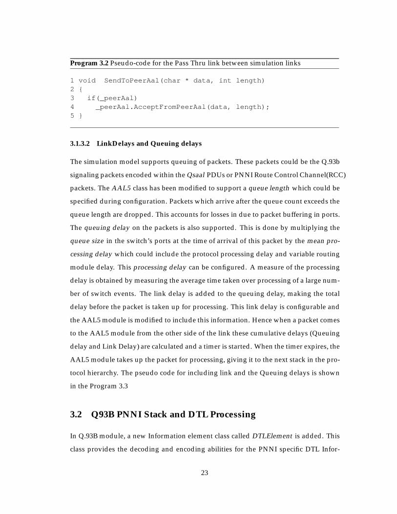
3.1.3.2 LinkDelays and Queuing delays
The simulation model supports queuing of packets. These packets could be the Q.93b
signaling packets encoded within the Qsaal PDUs or PNNI Route Control Channel(RCC)
packets. The AAL5 class has been modified to support a queue length which could be
specified during configuration. Packets which arrive after the queue count exceeds the
queue length are dropped. This accounts for losses in due to packet buffering in ports.
The queuing delay on the packets is also supported. This is done by multiplying the
queue size in the switch’s ports at the time of arrival of this packet by the mean pro-
cessing delay which could include the protocol processing delay and variable routing
module delay. This processing delay can be configured. A measure of the processing
delay is obtained by measuring the average time taken over processing of a large num-
ber of switch events. The link delay is added to the queuing delay, making the total
delay before the packet is taken up for processing. This link delay is configurable and
the AAL5 module is modified to include this information. Hence when a packet comes
to the AAL5 module from the other side of the link these cumulative delays (Queuing
delay and Link Delay) are calculated and a timer is started. When the timer expires, the
AAL5 module takes up the packet for processing, giving it to the next stack in the pro-
tocol hierarchy. The pseudo code for including link and the Queuing delays is shown
in the Program 3.3
3.2 Q93B PNNI Stack and DTL Processing
In Q.93B module, a new Information element class called DTLElement is added. This
class provides the decoding and encoding abilities for the PNNI specific DTL Infor-
23
Page 33
Program 3.3 Pseudo-code for Queuing and link delays
1 void AcceptFromPeerAal(data, length)2 {3 if(_queueCount == _queueLength)4 {5 delete data;6 }7 else8 {9 delay = linkDelay + QCount*processingDelay;10 startQtimer;11 }12 }13 void QtimerExpired()14 {15 upperLayer.ProcessData(data, length);16 // The upper layer modules could be Q.93b or PNNI RCC modules17 }
mation element. The format of this information element is shown in Table 3.1. In
this format, length of designated transit list contents specifies the number of hops to
be followed to the destination. Current transit pointer indicates the offset of the cur-
rent node identifier in the list of the nodes. Logical node identifier gives the 22 byte
node identifier. The DTLElement class also provides functions to manipulate its data
structures uring processing of the information element in the setup message.
In the Q.93B module, another new class Q93B PNNI is added. This class provides
the Q.93b signaling stack support for PNNI signaling control channel communication
between the ports of two switches. This class provides the ability to decode the manda-
tory DTL element from the setup message and store the DTL element object thus cre-
ated in the setup message object which is provided to the switch call control for pro-
cessing. In the outgoing setup message, it ensures the presence of the DTL element.
It encodes this DTL element into the outgoing data stream. This class also takes care
of the presence of the connection identifier IE in the setup or call proceeding or the
connect messages. The connection identifier IE provides the information regarding
the VPI and VCI pair to be used on the link for the connection establishment. A brief
24
Page 34
8 7 6 5 4 3 2 11 Coding IE Instruction Field
ext standardLength of designated transit list contents
Length of designated transit list contents(continue)Current transit pointer
Current transit pointer(continued)0 0 0 0 0 0 0 1
Logical node / Logical port indicatorLogical node identifierLogical port identifier
Table 3.1: Designated transition List
explanation is given for terms master-node and slave-node before looking into the rule
to be followed for processing connection-identifier
Among two adjacent nodes in PNNI, the master-node is the one whose node iden-
tifier is numerically greater than the peer node’s node identifier. The slave-node is
the node whose node identifier is numerically less than its peer node’s identifier. This
information is obtained when the two nodes exchange hello messages through their
route control channels before exchanging topology messages.
The rule to be followed while sending the connection-identifier is that the master-
node is the node which allocates the connection identifier for the link between the two
nodes. The following events which are supported in the Q93B PNNI class ensure that
the above rule is satisfied.
If the master-node receives the setup message from the slave, then the setup mes-
sage does not include the connection-identifier. When the master node sends out call-
proceeding or the connect message to the slave in reply to the setup message, the con-
nection identifier is a mandatory element in the connect message if call-proceeding is
not sent before it. Otherwise if the call-proceeding message is sent, the connection-
identifier must be included in it.
If the slave-node obtains the setup message first, then the connection-identifier
must be present in it. When the slave-node sends the response messages call proceed-
25
Page 35
ing or the connect, the connection-identifier must be omitted.
3.3 Switch Call Control Support for PNNI
Changes have been made in the switch call control to accommodate the PNNI signaling
and the routing. The changes could be listed as follows:
1. Support is provided to indicate if the destination host is connected to this node
or not. This function compares the 13 byte destination ATM address with the 13
bytes of the node identifier. If they are the same, it is decided that destination
host is connected to the same switch and a request is sent for the router table
which stores the host’s port number.
2. If Condition 1 fails then the destination address is compared with this node’s
peer group identifier mask and if it succeeds, then it is decided that the destina-
tion is present in the same peer group represented by this switch but not present
on this switch. A request is sent to the PNNI routing module for seeking the
source route to the destination.
3. If Condition 2 fails, then the destination is in another peer group and the call is
terminated.
The routing in the switch call control is changed to seek the routing request in the
following way.
� If the setup message is from a peer PNNI node, then the request for routing is
sent to the newly implemented PNNI router. These are the parameters provided
to the PNNI router whenever a routing request is made to the PNNI routing
service.
– The destination address.
– The QoS requirements regarding PCR, SCR, CDV, CTD and CLR.
– The designated transition list.
26
Page 36
– Incoming port number
� If the setup is received from a peer host and destination host is connected to the
same switch, the request is sent to the router table. Otherwise the request is sent
to the PNNI routing service.
3.4 PNNI Routing Services (PNNI RS)
A new interface module called PNNI Routing Service is added in Q.Port. This inter-
face provides interaction between the PNNI specific dynamic routing service and the
Switch Call Control(SCC). It also provides interface to the AAL5 submodule for the
purpose of Routing Call Control Channels. PNNI RS has a server-client relationship
with the SCC. SCC is the client, requesting routing services from the server PNNI RS.
3.4.1 Interaction between PNNI RS and SCC
The message interaction between PNNI RS and SCC is as shown in the Figure 3.3
SCC PNNI ROUTING SERVICEQ93B
SETUP
ROUTE_REQ
ROUTE_RESP
RELEASE
RELEASE_BW
PNNI
DYNAMIC
ROUTING
SERVICE.
Figure 3.3: Interaction between SCC and PNNI RS Modules
The messages are described below:
27
Page 37
� route req message: This message is a routing service request from the SCC to the
PNNI RS. There could be two categories of routing requests. They are:
– dtl request : This request is issued by the SCC when a setup message is
received from a host machine and the destination is not connected to this
switch. The PNNI RS will obtain the whole route to the destination which
satisfies the QoS, and then provides the DTL to the SCC.
– dtl parsing request : This request is issued by the SCC when a setup mes-
sage comes from a peer PNNI node which will have DTL in it. The PNNI
RS will check if the top of the DTL stack is this node itself. If so, it obtains
the output portnumber for the next hop.
� route resp message: This message is a response from the PNNI RS to a route
request message from the SCC. There could be five categories of responses in this
message which are:
– destination in same switch : This indicates that the request has been found
to satisfy QoS requirements for the input port so the call can be accepted. It
also indicates that the destination is in the same switch. When the SCC finds
this response, it requests the destination port from the local router table.
– call routed : This indicates that a path to the destination has been found and
the DTL is included for the path. It also provides the output portnumber to
which the SCC forwards the call.
– no bandwidth on incoming port : This indicates that the route request failed
due to unavailability of bandwidth on the incoming link and hence the call
cannot be routed.
– no bandwidth on outgoing port : This indicates that the there is no band-
width available on the outgoing port to support the requested bandwidth
and hence the call request is rejected.
– no route available : This indicates that no single path could be found which
satisfied all the QoS requirements all the way to the destination. Hence the
call request is rejected.
28
Page 38
� release bw message: This message is sent by the SCC when a release message is
obtained from one of the parties involved in the call. The PNNI RS, releases the
resources specified for this call and if required sends out topology messages to
the other nodes.
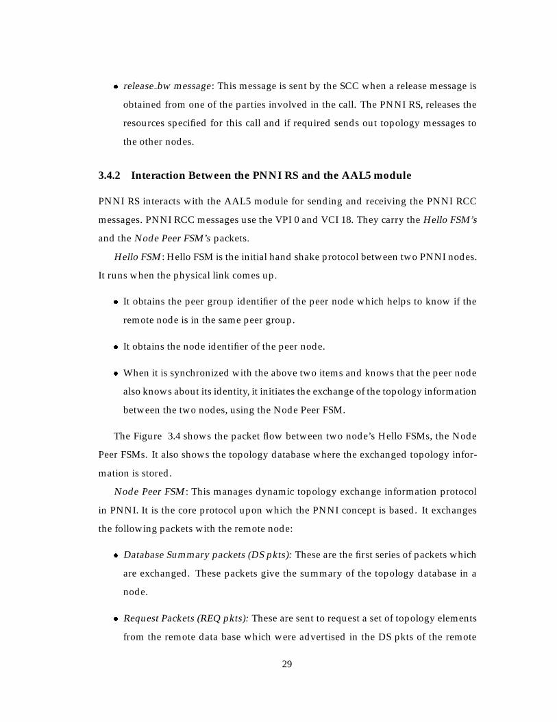
3.4.2 Interaction Between the PNNI RS and the AAL5 module
PNNI RS interacts with the AAL5 module for sending and receiving the PNNI RCC
messages. PNNI RCC messages use the VPI 0 and VCI 18. They carry the Hello FSM’s
and the Node Peer FSM’s packets.
Hello FSM: Hello FSM is the initial hand shake protocol between two PNNI nodes.
It runs when the physical link comes up.
� It obtains the peer group identifier of the peer node which helps to know if the
remote node is in the same peer group.
� It obtains the node identifier of the peer node.
� When it is synchronized with the above two items and knows that the peer node
also knows about its identity, it initiates the exchange of the topology information
between the two nodes, using the Node Peer FSM.
The Figure 3.4 shows the packet flow between two node’s Hello FSMs, the Node
Peer FSMs. It also shows the topology database where the exchanged topology infor-
mation is stored.
Node Peer FSM: This manages dynamic topology exchange information protocol
in PNNI. It is the core protocol upon which the PNNI concept is based. It exchanges
the following packets with the remote node:
� Database Summary packets (DS pkts): These are the first series of packets which
are exchanged. These packets give the summary of the topology database in a
node.
� Request Packets (REQ pkts): These are sent to request a set of topology elements
from the remote data base which were advertised in the DS pkts of the remote
29
Page 39
NP FSM NP FSM
HELLO
FSM
HELLOFSM
DS, REQ, PTSP,
ACK PKTS
PACKETS
HELLO
port port
Link
TopologyDatabase
TopologyDatabase
Figure 3.4: Hello and Node Peer FSMs
30
Page 40
LINK_UP
UDATA_REQ
UDATA_IND
PNNI ROUTING SERVICE AAL5
Figure 3.5: Messaging between PNNI RS and AAL5
node.
� PTSP packets (PTSP pkts): These are the topology information carrying packets.
They are sent out when a request is made by the peer node for specific topology
information or periodically when significant topology changes occur.
� Ack Packets (ACK pkts): These are the acknowledgements to the topology pack-
ets sent by the peer node.
The interface between the AAL5 and the PNNI RS module is shown in Figure 3.5
These messages are explained below.
� Linkup message: When the AAL5 module establishes the TCP connection with
the remote node, it sends the Linkup message to the PNNI service indicating that
the physical link is up and ready for data transfer.
� udata req: When the PNNI RS wants to send out any RCC packet stream to to the
remote node, it sends the udata req message to the remote node with a pointer
to the packet data stream.
� udata ind. When the AAL5 obtains packet data stream from the remote node, it
sends udata ind message to the PNNI RS.
31
Page 41
3.4.3 PNNI Routing Module’s Functionalities
The PNNI routing module is based on the PNNI routing software called ProuST de-
veloped by the the Naval Research Laboratory. This software, when interfaced with
the Q.Port signaling software, needed to be changed significantly first in order to get
the ProuST architecture fit over the Q.Port architecture and later to have the additional
functionalities to support PNNI single peer group experimentation. A summary of the
changes is explained here.
Part of the architectural changes included were discussed in the form of the PNNI
Routing service interface provided between the Q.Port modules SCC, AAL5 and the
PNNI routing modules in the Section 3.4. In addition to these changes, the timers in
the routing modules were changed to make use of the Q.Port supported timers. The
timer handling of the modules is changed to use the Q.Port style of timer handling.
All the modules were detached from the ProuST kernel support and were registered to
the Q.Port reactor scheduling and underlying passMT module. Most of the underlying
Design Pattern Frame Work of Proust software is retained for the intra-ProuST module
communication. In bringing up the PNNI routing module, some of the modules which
were redundant in case of the Q.Port architecture are eliminated. Important amongst
them are the Q93B signaling stack and associated information elements, queues, and
the modules simulating the links between switches. These are replaced by appropriate
Q.Port modules in the unified architecture. One of the important changes made was
in the routing of the data from the PNNI Routing Service to the Control modules of
the ProuST architecture. The complex inter-module routing facility which is present
in ProuST for provide the abilities a switch requires, is simplified to just providing the
routing service in the context of Q.Port.
The following additional functions were provided in the PNNI routing service.
� Convergence Time: Convergence time is the time taken by all the nodes in a peer
group to initially exchange the topology information and to be synchronized with
it. It helps to know about the arrival rates of the connection requests the network
could sustain sensibly. Also it could help in learning about the peer group size.
In the Database module of the PNNI routing architecture, support for finding the
32
Page 42
convergence time is implemented. All the nodes involved in the experimentation
are configured with the number of initial topology information elements present
in the peer group. When the topology exchange is started the time is noted. When
the database has all the topology information present in the peer group through
exchange of information with other nodes, the convergence time is noted. The
effective convergence time is calculated as the time it took for the last node in the
peer group to achieve convergence.
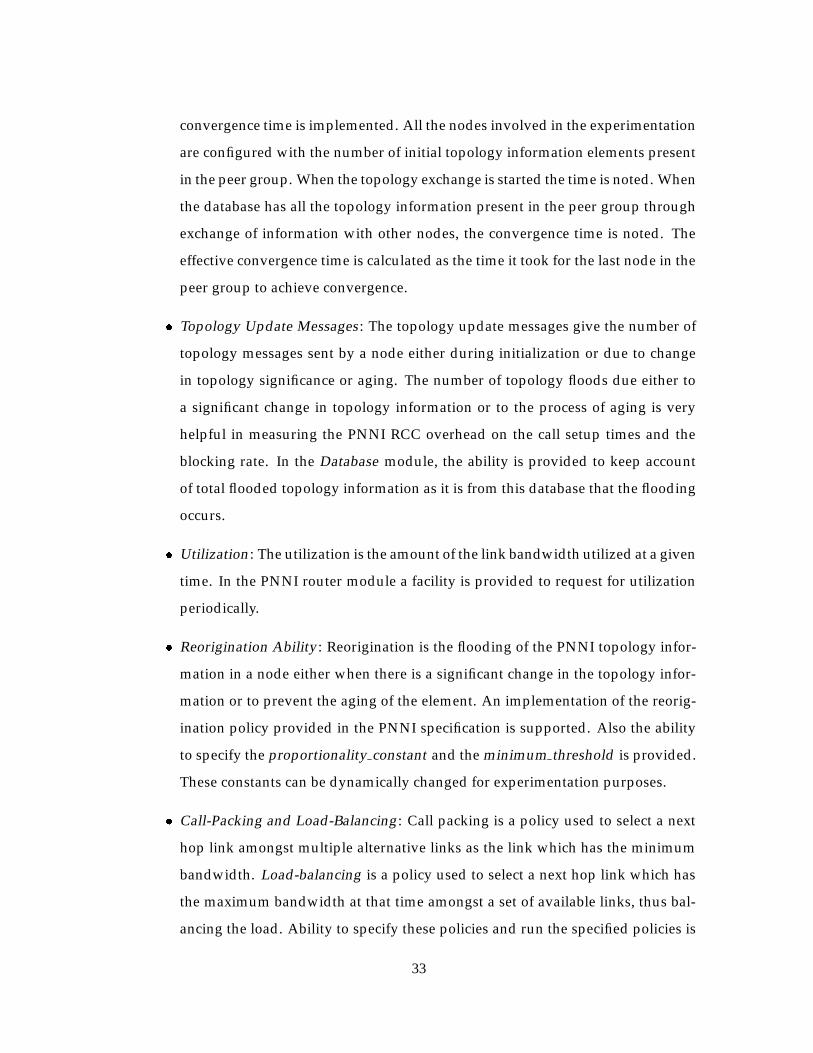
� Topology Update Messages: The topology update messages give the number of
topology messages sent by a node either during initialization or due to change
in topology significance or aging. The number of topology floods due either to
a significant change in topology information or to the process of aging is very
helpful in measuring the PNNI RCC overhead on the call setup times and the
blocking rate. In the Database module, the ability is provided to keep account
of total flooded topology information as it is from this database that the flooding
occurs.
� Utilization: The utilization is the amount of the link bandwidth utilized at a given
time. In the PNNI router module a facility is provided to request for utilization
periodically.
� Reorigination Ability: Reorigination is the flooding of the PNNI topology infor-
mation in a node either when there is a significant change in the topology infor-
mation or to prevent the aging of the element. An implementation of the reorig-
ination policy provided in the PNNI specification is supported. Also the ability
to specify the proportionality constant and the minimum threshold is provided.
These constants can be dynamically changed for experimentation purposes.
� Call-Packing and Load-Balancing: Call packing is a policy used to select a next
hop link amongst multiple alternative links as the link which has the minimum
bandwidth. Load-balancing is a policy used to select a next hop link which has
the maximum bandwidth at that time amongst a set of available links, thus bal-
ancing the load. Ability to specify these policies and run the specified policies is
33
Page 43
implemented.
� Selective routing policy: Using Dijkstra’s shortest path algorithm, the ability to
specify the cost function is provided.
The three policies based on the cost functions are,
– minimum hop policy: This is a distance vector policy where all the links
have the same cost associated with them.
– maximum bandwidth policy: This is a policy where the links are provided
with costs based on the amount of available bandwidth they have. The
higher the available bandwidth, the lower is the cost to traverse the link.
– minimum time policy: This is a policy where the links have cost based on
the link delay. The smaller the link delay the lower is the cost to traverse the
link.
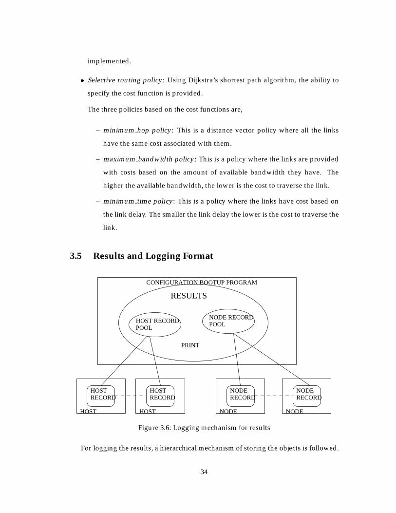
3.5 Results and Logging Format
RESULTS
HOST RECORDPOOL
NODE RECORDPOOL
HOSTRECORD
HOSTRECORD
NODERECORD
NODERECORD
HOST HOST NODE NODE
CONFIGURATION BOOTUP PROGRAM
PRINT
Figure 3.6: Logging mechanism for results
For logging the results, a hierarchical mechanism of storing the objects is followed.
34
Page 44
The configuration boot up program has the main results object of the Results class.
This class has pools of objects of two other classes, which are,
� Host-Call-Record : which is used to store the host related call generation logs. A
unique HostCallRecord for a host also has an array of call records. The pseudo
code of this log record is given in Program 3.4. Each call record for a call has
details to show the status of the call which could be failed or successful, the type
of call(CBR, ABR, VBR, UBR), the start time , the setup time, the bandwidth used
and the cause of failure if the call failed.
� Node-Record : The NodeCallRecord is unique to a node and it stores a node’s
logs. The pseudo code of this log record is given in Program 3.5. The hops
stores the average number of hops taken by calls generated at this node. The
route computation time indicates the average time taken in running routing al-
gorithms. The utilization provides the utilization logs of the network at different
times. The convergence gives the time taken for achieving convergence at this
node. The floods provide the number of topology floods that were generated.
Program 3.4 Pseudo code for the host call record
1 class HostCallRecord2 {3 array of CallRecords;4 }1 class CallRecord2 {3 StateOfCall{ success, failure};4 Calltype { cbr, rtvbr, nrtvbr, abr, ubr};5 startTime;6 setupTime;7 call bandwidth request;8 call failure cause;9 }
As shown in Figure 3.6 the boot up program has an object pointer to a unique re-
sults object. When it creates the individual hosts, it creates a HostCallRecords object
and passes it to the corresponding host. When it creates the individual nodes, it creates
35
Page 45
Program 3.5 Pseudo code for the node call record
1 class NodeRecord2 {3 number of hops;4 route computation time;5 link utilization;6 convergence time;7 number of floods;8 }
a NodeRecords object and passes it to the corresponding node. During the experimen-
tation, each of the hosts and nodes collect the logs they created into their respective
logging objects. When the experimentation is complete, the boot-up program which
has the object pointer to all the host’s and node’s logging records, prints them for the
user.
3.6 User Input Interface
The simulator is provided with a user input script interface. Using this script interface,
the network of interest could be specified along with the experimentation logs to be
collected. The design for this utility is as shown in Figure 3.7
When the user specifies the network, a PNNI parser is used to parse the input and
store the input data into a data structure. There may be some default parameters left
out by the user and these are filled in the complete user input function. When the input
configuration is complete, the data structure is given to a simulation boot-up program,
which sets up the simulation.
3.7 Call Generator Changes
The simulator uses a Call Generator module to make call connection requests with the
nodes. The call generator is designed to request the connections in specified arrival
and duration distributions. The call generator parameters can be specified in a user
input script during experimentation. Thus the call generator is a very comprehensive
36
Page 46
USER INPUT
SCRIPT
PNNI
PARSER
SIMULATION
CompleteUserInput()
RUN
SIMULATION
DisplayResults()
Figure 3.7: Design of common interface to simulator and emulator
and is extended to generate realistic traffic in a big ATM network. The call generator is
provided with these capabilities.
The following call arrival distributions are supported:
� Poisson Distribution.
� Uniform Distribution.
� Periodic Distribution.
The following additional call arrival types are supported:
� Tear Down type: In this type of calls, when a call connection is established, it is
immediately torn down and the the next call is attempted.
� Burst Type: In this type calls, when a call connection is established, immediately
next call is attempted.
The following call duration distributions are supported:
� Poisson distribution.
37
Page 47
� Uniform distribution.
� Periodic distribution.
The following call traffic types are supported:
� CBR: Constant Bit Rate.
� ABR: Available Bit Rate.
� RTVBR: Real time Variable Bit Rate.
� NRTVBR: Non Real time Variable bit rate.
� UBR: Unspecified bit rate.
The following QoS parameters for connection request are supported:
� pcr : peak cell rate.
� scr : sustainable cell rate.
� ctd : Minimum cell transfer delay.
� cdv : cell delay variation.
� clr : cell loss ratio.
The call connections can be made to the following types of destinations.
� A single specified destination. Ex: destination1
� A range of destinations. Ex: destination1 to desitination10.
� Explicitly specified destinations. Ex: destination1 destination2 destination3
When the calls are generated to more than one destination, the destinations are selected
uniformally over the available destinations.
The call generator also supports multiple traffic sources with different QoS require-
ments being part of the total number of the calls generated. Here QoS requirements are
specified for individual sources. The number of calls generated of each traffic can be
38
Page 48
specified as percent share of total calls generated. When multiple traffic sources are
available, the calls are made with a single arrival distribution, while the duration dis-
tribution for each of the traffic sources can be different.
39
Page 49
Chapter 4
Evaluation
This chapter evaluates the work done to study the performance of a single peer group
PNNI protocol. It also evaluates the capacity of the simulator to simulate large scale
networks. The evaluation is done in the following 2 sections.
� Experiments with abstract topologies: Abstract topologies like ring, chain and
the mesh topologies are used in these experiments. The experiments regarding
the basic topology convergence time with these topologies is explained.
� Experiments with realistic topologies: Realistic edge-core topologies are used
in these experiments. Experiments regarding, PNNI proportional multiplier for
significant topology information change, call setup times, utilization, and topol-
ogy scaling are explained. The simulator’s performance study is also explained
in this section.
4.1 Experiments With Abstract Topologies
Sample chain, ring and the mesh topologies are shown in Figure 4.1. Some of the
features of these topologies are as follows: The chain topology has a higher diameter
than the ring topology. Here note that diameter is the maximum of the minimum
distances between all the two node pairs in the topology. Hence for the chain topology
shown in the figure, the diameter is 5 and for the ring topology it is 3. For the 9
node mesh topology the diameter is 4. The mesh topology has nodes connected with
40
Page 50
6 node ring topology
6 node chain topology
9 node mesh topology
Figure 4.1: Chain, Ring and Mesh topologies
different number of links with maximum number of links connected to a node being
4 and minimum 2. The experiments on convergence time and the topology update
messages generated for each of the topologies is explained in this section.
4.1.1 Topology Convergence Time
The topology convergence time is the time it takes for all the nodes in the network to
synchronize with initial topology information generated by each of the participating
nodes. The initial topology information generated by each node includes:
� Nodal Information: which gives information about the node identifier and peer
group of the node along with some node specific characteristics such as leader-
ship priority and others.
� Horizontal Link Information: This contains link information regarding band-
width, delay, and others. Each node advertises all the links to neighboring nodes.
These primary topology information elements are sufficient for routing a call connec-
tion request to any other node in the peer group.
41
Page 51
Convergence time is an important performance metric as it lets us know how quickly
topology information which is flooded could get through the different nodes in the net-
work and help all the nodes in the network have a common view of the network. The
convergence time depends upon the following factors:
� The size of the network.
� The connectivity density of the links between the nodes, which is number of links
between the nodes in a network.
� The processing capabilities of the nodes in the network.
� The link delay between the nodes in the network.
Following sections describe the convergence time experiments with each of the above
parameters.
4.1.1.1 Convergence Time With Increasing Number of Nodes
0 10 20 30 40 50 60 70 80 90 1000
1000
2000
3000
4000
5000
6000
nodes
conv
erge
nce
time(
ms)
Convergence time Vs Nodes
chainring mesh
(a) Convergence time with nodes
0 10 20 30 40 50 60 70 80 90 1000
1000
2000
3000
4000
5000
6000
7000
8000
Number of Nodes
Con
verg
ence
tim
e (m
s)
Convergence Times ranges Vs Nodes
chain highchain low ring high ring low mesh high mesh low
(b) Differing Convergence times
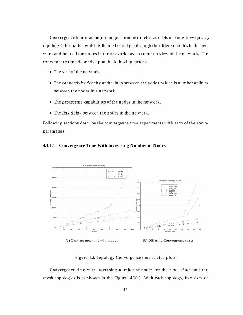
Figure 4.2: Topology Convergence time related plots
Convergence time with increasing number of nodes for the ring, chain and the
mesh topologies is as shown in the Figure 4.2(a). With each topology, five sizes of
42
Page 52
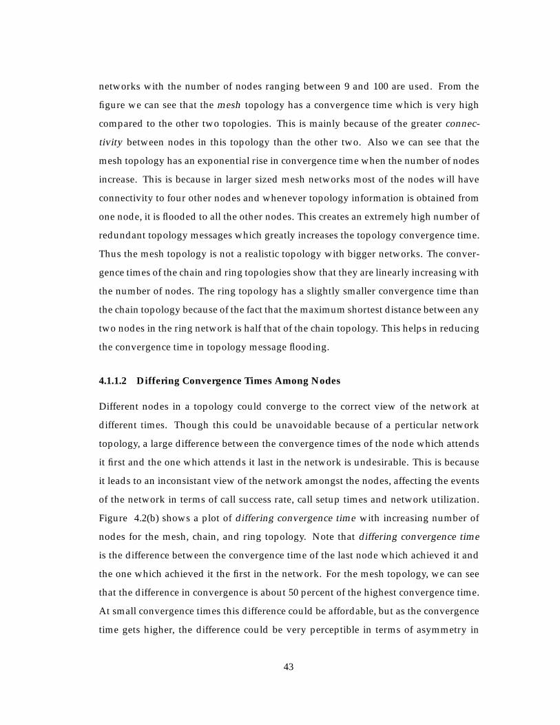
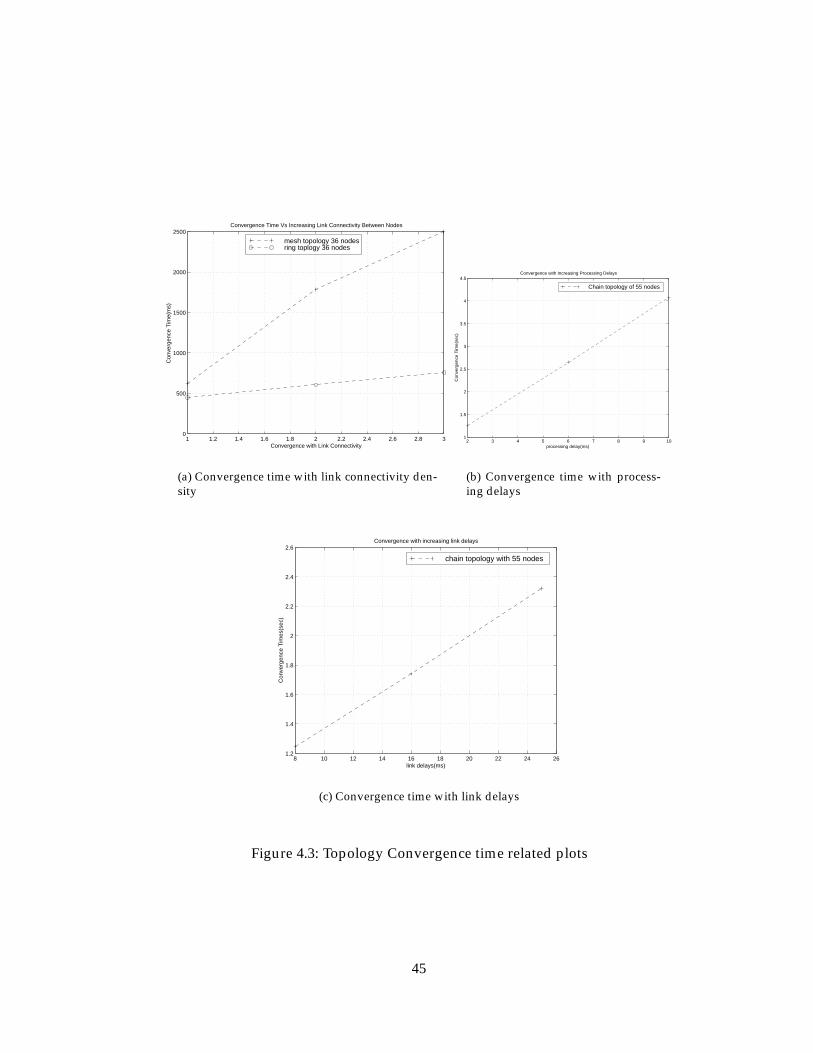
networks with the number of nodes ranging between 9 and 100 are used. From the
figure we can see that the mesh topology has a convergence time which is very high
compared to the other two topologies. This is mainly because of the greater connec-
tivity between nodes in this topology than the other two. Also we can see that the
mesh topology has an exponential rise in convergence time when the number of nodes
increase. This is because in larger sized mesh networks most of the nodes will have
connectivity to four other nodes and whenever topology information is obtained from
one node, it is flooded to all the other nodes. This creates an extremely high number of
redundant topology messages which greatly increases the topology convergence time.
Thus the mesh topology is not a realistic topology with bigger networks. The conver-
gence times of the chain and ring topologies show that they are linearly increasing with
the number of nodes. The ring topology has a slightly smaller convergence time than
the chain topology because of the fact that the maximum shortest distance between any
two nodes in the ring network is half that of the chain topology. This helps in reducing
the convergence time in topology message flooding.
4.1.1.2 Differing Convergence Times Among Nodes
Different nodes in a topology could converge to the correct view of the network at
different times. Though this could be unavoidable because of a perticular network
topology, a large difference between the convergence times of the node which attends
it first and the one which attends it last in the network is undesirable. This is because
it leads to an inconsistant view of the network amongst the nodes, affecting the events
of the network in terms of call success rate, call setup times and network utilization.
Figure 4.2(b) shows a plot of differing convergence time with increasing number of
nodes for the mesh, chain, and ring topology. Note that differing convergence time
is the difference between the convergence time of the last node which achieved it and
the one which achieved it the first in the network. For the mesh topology, we can see
that the difference in convergence is about 50 percent of the highest convergence time.
At small convergence times this difference could be affordable, but as the convergence
time gets higher, the difference could be very perceptible in terms of asymmetry in
43
Page 53
network view. For example, in the mesh topology with 100 nodes, the difference in
convergence time is about 3 seconds. If the average call interarrival time of the network
is less than 3 seconds, then the calls could be routed or rejected by the source nodes
with outdated topology information leading to inefficient use of network resources
which is undesirable. If we compare the ring and chain topology in the Figure 4.2(b) it
is observed that the ring topology will form a better PNNI network topology than the
chain network, not only because its convergence time is small, but also the difference
in the convergence time amongst the participating nodes is less.
4.1.1.3 Convergence Time With Varying Connectivity Density
The convergence time also increases with the connectivity density between the nodes.
The connectivity density experiments were conducted with one, two, and three links
between any two nodes in the networks. Mesh and ring topologies, both with 36 nodes,
were used for the experiments. Figure 4.3(a) shows that the for mesh and ring topolo-
gies the convergence time increased linearly with the increasing connectivity densities.
Since for each link there are two topology messages originated, one by each side of the
link, adding new links causes additional topology messages in the network and hence
increased convergence time. It is undesirable to have a higher convergence time for
this sake. This shows that it would be better to have fewer links with more bandwidth
than the other way around. This is the concept which is used in multiple peer group
PNNI by aggregating links between the peer groups to reduce the topology informa-
tion flooding.
4.1.1.4 Convergence Time With Varying Processing Delays
This is an attempt to see how the convergence time could be affected with different
message processing delays for the nodes. Processing delays of 2ms, 6ms and 10ms
were tried on a chain topology of 55 nodes. Figure 4.3(b) shows that we get a linear rise
in convergence time with the increasing processing delays. This is an interesting issue
as in a network we could have nodes with different processing delays. Some network
providers offer two types of switches which differ in processor capabilities by a factor
44
Page 54
1 1.2 1.4 1.6 1.8 2 2.2 2.4 2.6 2.8 30
500
1000
1500
2000
2500
Convergence with Link Connectivity
Con
verg
ence
Tim
e(m
s)
Convergence Time Vs Increasing Link Connectivity Between Nodes
mesh topology 36 nodesring toplogy 36 nodes
(a) Convergence time with link connectivity den-sity
2 3 4 5 6 7 8 9 101
1.5
2
2.5
3
3.5
4
4.5
processing delay(ms)
Con
verg
ence
Tim
e(se
c)
Convergence with Increasing Processing Delays
Chain topology of 55 nodes
(b) Convergence time with process-ing delays
8 10 12 14 16 18 20 22 24 261.2
1.4
1.6
1.8
2
2.2
2.4
2.6
link delays(ms)
Con
verg
ence
Tim
es(s
ec)
Convergence with increasing link delays
chain topology with 55 nodes
(c) Convergence time with link delays
Figure 4.3: Topology Convergence time related plots
45
Page 55
of five. If we have such switches in the same network, then the convergence times they
achieve could differ and lead to some inconsistencies in terms of the network behavior.
Hence it is better to avoid having two different nodes exposed to similar network traffic
with differing processing capabilities. At the same time, a core node supporting many
edge nodes could benefit form higher processing capability.
4.1.1.5 Convergence Time with Varying Link Delays
The convergence time changes with increasing link delays. Link delays of 8, 16 and 26
ms were tried between the links in a 55 node chain topology. Figure 4.3(c) shows that
the convergence time increases linearly with increasing link delay. Bigger link delays
signify bigger networks and so the network should be carefully designed to limit the
peer group size when convergence times become large.
4.1.2 Topology Updates With Different Network Topologies
The simulation tool can be instrumented to log the number of PNNI topology update
messages sent by each node during topology synchronization. Figure 4.4(a) shows the
topology update messages for the ring, chain, and the mesh topologies during conver-
gence. From the figure it is apparent that the update messages increase linearly for the
ring and chain topologies with increasing nodes. For the mesh topology, the number of
update messages becomes extremely high with the increasing nodes. This is because
the redundancy of flooded messages increases in the mesh topology where most of
the nodes are connected to four other nodes. In ring and chain topology, each node
is connected to only two other nodes. In the mesh topology, nodes flood information
amongst themselves, increasing the redundantly flooded messages. This can be seen
in Figure 4.4(b). For the mesh topology, it is observed that more than half of the mes-
sages are redundant messages. More interconnectivity between nodes helps reduce
the convergence time of the network. But having half of the messages being redun-
dantly flooded, the performance of a mesh network decreases with increasing network
size. The average link bandwidth consumed during topology convergence is shown
in 4.4(c). It can be observed from the figure that the ring topology has a higher band-
46
Page 56
0 10 20 30 40 50 60 70 80 90 1000
2
4
6
8
10
12
14x 10
4
Number of nodes
PN
NI t
opol
ogy
mes
sage
s
PNNI topology messages Vs nodes
chainring mesh
(a) Topology messages
0 10 20 30 40 50 60 70 80 90 1000
2
4
6
8
10
12
14x 10
4
number of nodesP
NN
I top
olog
y up
date
mes
sage
s
Redundant topology updates Vs nodes
total ring redundant ringtotal mesh redundant mesh
(b) Redundant messages
0 10 20 30 40 50 60 70 80 90 100250
300
350
400
450
500
550
600
650
Number of Nodes
Ave
rage
topo
logy
mes
sage
ban
dwid
th p
er li
nk(a
tm c
ells
/sec
) 1c
ell =
53
byte
s
PNNI topology message bandwidth Vs Nodes
chainring mesh
(c) Bandwidth occupied by topology messages
Figure 4.4: Topology message flooding related plots
47
Page 57
width consumption than the mesh topology. This is because in the ring topology the
links to nodes ratio is equal, which is not true of the mesh topology. In the mesh topol-
ogy, because of higher connectivity density, more links share the topology messages
reducing the per link bandwidth. The ring topology has higher topology bandwidth
per link than the chain topology because of the redundant messages. This is reflected
in a smaller convergence time for the ring topology than the chain topology. In a chain
topology there are no wasted messages. Figure 4.4(b) shows the redundant messages
for the ring topology. In the ring topology we can see that the redundant messages are
a very small fraction of the total topology messages. But the ring topology performs
better compared to chain topology by reducing the convergence time to half that of the
chain topology.
4.2 Experiments With Realistic Topologies
The popular Edge-Core topology which is mostly used in setting up a private ATM net-
work is used. The model topology used is explained in section 4.2.1. The experiments
with this topology are based on the following studies:
� The study regarding proportionality multiplier which is used to calculate the
significant changes in the topology information before flooding them.
� Link utilization improvement study.
� Different routing policy study.
� The performance of the PNNI protocol with the expanding networks.
� Performance of the simulator.
4.2.1 Topology description
For experimentation purposes an edge-core topology of 45 nodes is considered as
shown in Figure 4.5. This will be labelled as the Model topology. In this topology, core
nodes are connected to other core nodes. Each core node connects to 2 edge nodes.
48
Page 58
Each edge node connects to a host which generates the calls. Depending upon the den-
sity of connectivity of the core nodes with the other core nodes, they are divided into
three categories.
� A Large range node which connects to other larger nodes to support the long
distance traffic.
� A middle range node which connects to other middle range nodes to support
medium range traffic.
� A small range node which depends upon the adjacent long and the middle range
nodes for long and medium range traffic.
These three categories of nodes are identified by the letter L for Large range node, M
for Middle range node, and S for small range node. The edge nodes are denoted with
the letter E and the hosts are denoted with the letter H. In the topology each of the core
nodes is connected to 2 edge nodes and each edge node is connected to a host node. In
the figure, multiple edge nodes and hosts are avoided for simplicity. The numbers on
each of the links specify the link delays in milliseconds.
The link delays between core nodes are chosen so that large scale nodes are pre-
ferred for long distance connections and middle scale nodes for middle distance con-
nections, though it may not happen this way necessarily depending upon the traffic
and network conditions. The topology supports a maximum round trip time of about
45 milliseconds. The link bandwidth between different nodes and hosts is shown in
Link bandwidth(Mbps)core to core 155edge to core 2000edge to host 2000
Table 4.1: Link bandwidths for different links
The host to edge node and the edge node to core node link bandwidths are kept
at very high values to avoid bottleneck bandwidths at these links and thus helping
to exploit the core bandwidth in the network. Note that the bandwidth in the links
49
Page 59
.
L
LL
L
LL
M
S
S
S
S
S
M
M
M
M
EE
H
1
1
1
3
5
4 3
5
4
3
5
43
54
3
5
4
6
12
12
6
7
7
7
7
7
6
6
6
1212
12
H
12
1
Figure 4.5: Edge core topology of 45 nodes
50
Page 60
between edge node and core nodes and the links between the edge node and a host
is chosen to be very high which is not realistic, but it helps avoiding congestion at
the edge itself which could have limited the scope of the this experimentation to the
edge of the network. The call generation related arrival distributions, the duration
distributions and QoS parameters for the calls are given in Table 4.2. Multiple traffic
types are used during call generations to ensure a variety in bandwidth requirements.
All the hosts generate calls to all the other hosts in the network with the destinations
being selected in uniform distribution from the whole range of the hosts. All the hosts
use different random number seeds to generate the call connection requests, select the
destinations and select the call duration times, ensuring different traffic patterns from
different hosts. The total number of calls generated per experimentation are about 6000
calls with different call arrival rates with Poisson mean of 5sec and 2sec for each host.
This gets the average network call arrival rates of 6 and 15 calls/sec respectively. These
measures and capabilities help simulate a traffic which is close to that in a real ATM
network. These parameters are used with all the experiments under this section.
SOURCE BANDWIDTH DURATION(sec) PERCENTAGE OF CALLSCBR1 2Mbps uniform[10, 40] 40CBR2 4Mbps uniform[20, 50] 40CBR3 8Mbps fixed 50 20
Table 4.2: Call sources and QoS requirements
4.3 Call Generation Experiments Related To Proportional Mul-
tiplier
The Proportional multiplier is a parameter which is used to determine the significance
of change of link bandwidth with respect to the previously available bandwidth on
the link. It helps in obtaining a lower and higher bound for the next available band-
width. If the new call request or the released call, forces the link available bandwidth
to cross any of the two bounds, the change is considered significant and the horizontal
51
Page 61
link information is flooded amongst the other nodes. The algorithm for finding the
significance is given in PNNI specification [3]
4.3.1 PNNI Topology Update Messages
Figure 4.6 shows the PNNI topology update messages generated at different core nodes
in the network. From the figure it can be seen that the maximum number of messages
are generated in the large range core nodes and next in the middle range nodes and fi-
nally in the small range nodes. The wasted messages generated are also shown respec-
tively at each of the nodes. This confirms that the traffic pattern in the large, middle
range, and the small range nodes is on the expected lines.
1 2 3 4 5 6 7 8 9 10 11 12 13 14 150
2000
4000
6000
8000
10000
12000
14000
Node identity
topo
logy
upd
ates
Topology updates at different nodes in the network
1 to 5 are large range,6 to 10 are middle range,11 to 15 are short range nodes
Total messages Redundant messages
Figure 4.6: Topology update messages
52
Page 62
4.3.2 PNNI Topology Messages With the Different Proportional Multiplier
Values
Proportional multiplier(prop mult) values of 25, 50 and 75 are used to calculate the sig-
nificant changes in the topology information. Figure 4.7(a) shows the total topology
flood messages generated. We can see that with the decreasing proportionality multi-
plier, we have increasing numbers of topology messages. At prop mult of 25 we can
see three times more messages generated than with the prop mult of 75. This is because
of the lower significance of change of information crieteria for flooding the topology
information at a lower proportional multiplier. More updates will lead to frequent con-
vergence amongst the nodes in the network and this is helpful if the inter-call arrival
time is less than the time it takes topology information originated in a node to reach
all the other nodes in the network. Figure 4.7(a) also shows the topology updates
generated at a Poisson mean of 2sec per host. More topology updates are observed
here because at 2sec/call, with 30 hosts, the average call arrival rate for the network is
around 15calls/sec and this results in some of the core links getting fully utilized dur-
ing high traffic conditions and resulting in increased floods. Note that when the links
get utilized to a higher extent, a small change in link bandwidth leads to a significance
change, resulting in flooding of the topology information.
Figure 4.7(b) shows the average topology updates per call with respect to different
prop mult values. We can observe that, as expected with a lesser prop mult, value,
more updates per call are generated than at a higher prop mult value. Also, with a
mean Poisson call arrival of two we find slightly more updates per call than at Poisson
mean of five, which is as expected. More topology updates per call could lead to higher
call setup times.
4.3.2.1 Average Call Setup Times
Figure 4.8(a) shows the average call setup times with three different values for prop mult.
There are two plots showing the mean Poisson call arrivals means at 5sec and 2 sec per
host. While comparing the call-setup times at call arrival rates with a Poisson mean
of 2sec, for different values of prop mult we can see that at prop mult = 25 we get the
53
Page 63
25 30 35 40 45 50 55 60 65 70 750
2
4
6
8
10
12
14
16
18x 10
4
proportional multiplier
Top
olog
y up
date
mes
sage
s
PNNI topology updates Vs proportional multiplier, 45 nodes, 30 hosts
Total updates, Arrival Poisson mean /host = 5 sec Total updates, Arrival Poisson mean /host = 2 sec Redundant updates, Arrival Poisson mean /host = 5 secRedundant updates, Arrival Poisson mean /host = 2 sec
(a) Topology messages with changing propor-tional multiplier
25 30 35 40 45 50 55 60 65 70 750
5
10
15
20
25
proportional multiplier
topo
logy
upd
ates
per
cal
l
Topology updates per call Vs proportional multiplier
avg poisson mean for arrival = 5 secavg poisson mean for arrival = 2 sec
(b) Topology update messages percall
Figure 4.7: Topology message flooding related plots in Model topology
highest average call setup time of about 120ms compared to the lowest average call
setup time of 90ms for the prop mult = 75. This is because of the larger number of
topology updates generated with prop mult 25 than with prop mult 75, affecting the
call-setup times. When comparing call setup times at different call arrival rates, we
can see that with a Poisson mean of 5sec the call setup times scale down to about 50%
of the setup times at Poisson mean of 2sec. This is because of the cumulative effect of
increased interleaving among the calls requests, and also due to the resultant topology
floods generated.
4.3.2.2 Failed Calls Amongst the Calls Generated
The type of failed calls will let us know if there is a convergent view in the network.
Failed calls are distinguished as:
� Source node failed calls( SFCs): These are the calls which failed at the source
node itself due to non-availability of the route which satisfies the bandwidth re-
quirements of the call.
54
Page 64
� Intermediate node failed calls(IFCs): These are the calls which failed at an inter-
mediate node due to non-availability of the bandwidth for the call.
This is an important distinction because a larger percentage of SFCs in the failed calls
indicates that the nodes have converged so that the source node knows the unavail-
ability of the bandwidth for the call. Larger percentage of IFCs in the calls indicates
non convergence, as the source nodes accept the call and send it to a destination only
to have an intermediate node reject it. This is an important metric to limit the network
size for a single peer group. Figure 4.8(b) shows the failed calls in the experimentation
with regards to the Poisson arrival mean of 2 sec per host. From the figure, it can be
seen that about 90% of the failed calls are SFCs. This indicates that this topology of 45
nodes is convergent and can be used for a single peer group network.
25 30 35 40 45 50 55 60 65 70 7570
75
80
85
90
95
100
105
110
115
120
proportional multiplier
Cal
l set
up ti
me(
ms)
Average Call setup time Vs prop_mult
total hosts = 30 in 45 node network
Arrival Poisson mean per host = 5 secArrival Poisson mean per host = 2 sec
(a) Avg Call-setup times
25 30 35 40 45 50 55 60 65 70 750
10
20
30
40
50
60
70
80
90
100
proportionality multiplier
%sh
are
of s
ourc
e an
d in
term
edia
te fa
iled
calls
% share of source and intermediate node failed calls
Plot compares the source node and intermediate nodefailed calls as a fraction of the total failed calls
Poisson arrival mean per host = 2 sec
Source node failed calls Intermediate node failed calls
(b) Failed calls
Figure 4.8: Call setup time and Call failure plots
4.3.2.3 Bandwidth Rejection of The Calls
With the simulation tool, we can also log the amount of the bandwidth rejected. Per-
centage bandwidth rejected could be different from the percentage of rejected as calls
could request different bandwidths. The call bandwidth rejected is shown in Figure
55
Page 65
4.9(a). From the figure it is observed that at Poisson arrival rates of 2sec per host about
64 % of the bandwidth is rejected at a prop mult of 75. This is because there were about
15 bottleneck links which were occupied to the full bandwidth during some time or
other during the simulation. The percentage call rejection is shown in Figure 4.9(b).
From the experiments, it is observed that using prop mult at 25, though the network
creates more topology messages, it maintains better synchronization because of the
quick convergence. Hence, 25 is a better suited value for prop mult. Using the value of
25 for prop mult has a higher value of average call setup time, but better percent call
success.
25 30 35 40 45 50 55 60 65 70 750
5
10
15
proportional multiplier
CB
R b
andw
idth
rej
ectio
n(M
byte
s)
Bandwidth rejection Vs prop_mult at different arrival rates
Arrival Poisson mean per host = 5secArrival Poisson mean per host = 2sec
(a) Call bandwidth rejection
25 30 35 40 45 50 55 60 65 70 750
10
20
30
40
50
60
70
proportional multiplier
% c
all r
ejec
tion
Percent call rejection Vs proportionality multiplier
Arrival Poisson mean per host = 5 secArrival Poisson mean per host = 2 sec
(b) Percent call rejection
Figure 4.9: Call Rejection and Bandwidth Rejection Plots
4.4 Improvement In Percent Call Success Rate
Figure 4.10(a) shows the average utilization on some of the links. We can see that
the links connecting the short range and long range nodes are more utilized than any
other links. The links between the long range to long range nodes are the least utilized.
When the simulations were run with a call arrival rate with a Poisson mean of 5sec
56
Page 66
it was found that about 20 links which are mainly connecting the short to long range
nodes with delay of 3ms(refer to Figure 4.5), connecting the short to middle range
nodes with delay of 5ms, or connecting the long to middle range nodes with delays of
4ms were found to be fully utilized at sometime during the simulations, causing call
rejections. This was producing a call success rate of about 70 % . Then, in the next
run of the simulation these identified bottleneck links were given a bandwidth of oc12
instead of oc3. With the increased bandwidth, a 100 % call success rate was achieved
as shown in Figure 4.10(b).
1 2 3 40
0.1
0.2
0.3
0.4
0.5
0.6
0.7
Link identity
Avg
Util
izat
ion
The link utilization for different links − utilization experiment
x axis details1 = link between long to short nodes2 = link between long range nodes3 = link between short to medium range nodes4 = link between long to medium range nodes
Link bandwidth = 155 Mbps
(a) Utilization
1 20
10
20
30
40
50
60
70
80
90
100
Experiments identity which differ in core link bandwidth
%ca
lls s
ucce
eded
% Call success for oc3 and oc12 bandwidths for selected core links
x axis details1 = % calls accepted with 20 heavily utilized oc3 links2 = % calls accepted by increased link bandwidth to oc12
total calls = 6000
(b) Call Success Improvement
Figure 4.10: Utilization and Call success improvement
4.5 Routing with Different Routing Policies
Using the simulation tool, different routing policies can be selected to route a call. The
experiments were run for 15000 calls with Poisson arrival mean of 5sec per host. The
following policies were used.
� minimum time: Link delay is used as the cost function in calculating the route.
The higher the link delay, the higher the cost.
57
Page 67
� maximum bandwidth : Maximum available bandwidth is used as the cost func-
tion. The higher the bandwidth the lesser the cost.
� minimum hops: Minimum available bandwidth is used as the cost function. All
the links are allocated a fixed value of 1 for the cost of the link.
� minimum bandwidth : Minimum bandwidth is used as a cost function. The
lesser the available bandwidth, the lesser the cost.
Figure 4.11 shows the Call success rates in the policies used. The minimum-time
and the maximum bandwidth policies performed the best with about 90% call suc-
cess. Minimum-hop policy and the minimum-bandwidth policies didn’t perform well.
The minimum- hop policy performs badly because it always selects the same shortest
path which could lead creating a bottleneck link. Minimum-bandwidth performs the
worst with 70 % call success.
1 2 3 40
10
20
30
40
50
60
70
80
90
100
Routing Policies
% s
ucce
ssfu
ll ca
lls
% Call success for different routing policies
x axis details
1 = minimum time policy2 = maximum bandwidth policy3 = minimum hop policy4 = minimum bandwidth policy
total calls = 15000
Figure 4.11: Call Success with different routing policies
58
Page 68
4.6 The Performance of the PNNI Protocol with Expanding Net-
works
To compare the performance of the single peer group PNNI network with an expand-
ing network size, three different sizes of core edge network topology are chosen. They
are of the sizes:
� 12 nodes: 4 core, 8 edge nodes, 8 hosts.
� 45 nodes: 15 core, 30 edge nodes, and 30 hosts.
� 120 nodes: 40 core, 80 edge nodes, and 80 hosts.
Figure 4.12(a) shows the average number of hops of a connection with respect to the
total nodes. The average hops in a 45 node network is about 4 hops and that for a 120
node network is about 5.5. This shows that though the networks get bigger, they are
interconnected in such a way that the average number of hops does not increase lin-
early, thus reducing the call setup time. For the edge core topology tested, the average
number of hops obtained seem appropriate. Figure 4.12(b) shows the call setup time.
This shows the tendency of a 120 node network to have larger setup times.
Figure 4.13(a) shows the percentage of the calls failed in the intermediate hops
in the network. There is a marked difference between the 120 node topology and the
other two. In the 120 node topology, about 70 percent of the failed calls are failing at the
intermediate nodes indicating a non-convergence amongst the nodes. A convergence
time for the 120 node network is shown in the Figure 4.13(b). The convergence time
of about 8 secondsconfirms the fact that it takes longer for the network to converge the
with the topology information. At Poisson arrival rates of 5 sec per host it could gener-
ate many topology elements resulting in continuously changing the network topology
information. Thus a 120 node network seems to be unsuitable for a single peer group
topology. This is a very important result in terms of deciding the topology size.
Figure 4.14(a) shows the average route computation time for the different net-
works. It is seen that in 12 and 45 node networks, the route computation time makes
59
Page 69
0 20 40 60 80 100 1202.5
3
3.5
4
4.5
5
Total number of nodes
Ave
rage
Num
ber
of H
ops
Average number of hops comparisons for 12, 45 and 120 node networks
(a) Average Hops
0 20 40 60 80 100 12040
60
80
100
120
140
160
Ave
rage
cal
l set
up ti
mes
(ms)
Avg call setup time comparisons for 12,45 and 120 node networks
Total number of nodes
(b) Average Setup times
Figure 4.12: Average hops and Call setup plots
0 20 40 60 80 100 1200
10
20
30
40
50
60
70
80
Total number of nodes
% o
f cal
ls fa
iled
at in
term
edia
te n
odes
% of calls failed at intermediate nodes for 12, 45 and 120 node networks
Poisson arrival rate/host = 5 sec45 node network total calls= 5500120 node network total calls= 6500
45 node network, source failed calls = 424, Intermediate failed calls =6
125 node network, source failed calls = 399, Intermediate failed calls = 1064
(a) Failed calls
0 20 40 60 80 100 1200
1
2
3
4
5
6
7
8
9
Total number of nodes
Top
olog
y co
nver
genc
e tim
e(se
c)
Comparison of topology convergence times in 25, 45, and 120 node networks
(b) Convergence time
Figure 4.13: Failed Calls and Convergence Time plots
60
Page 70
up a small part of the call setup time. Whereas in 120 node network, the route compu-
tation time is about 120ms - comparable to the call setup time. This is due to the time
required to cull through a graph of about 120 nodes and all the associated links. This
could be easily avoided by providing smaller peer group sizes. This is another reason
for believeing that a 120 node network is not suitable for a single peer group.
4.7 Performance of Simulator
The Figure 4.14(b) shows the slow down factor of the simulation at 12, 45 and 120
nodes. While at 12 nodes, the simulation runs faster than the real time, it slows down
by about four times at 45 nodes and about 35 times at 120 nodes. Slow down with the
larger networks is due to the size of the simulation network itself. Another important
reason for slowing down of the simulation is because of the increased PNNI topology
updates in bigger networks. These topology updates give much smaller simulation
time increment though a lot of them are processed. Considering the slow down factor
of about 35 for a network of about 120 nodes is supposed to be good, we can simulate
such a network.
0 20 40 60 80 100 1200
20
40
60
80
100
120
Total number of nodes
Avg time for route computation in 12,45 and 120 node networks
Ave
rage
rou
te c
ompu
tatio
n tim
es (
ms)
(a) Route computation time
0 20 40 60 80 100 1200
5
10
15
20
25
30
35
40
Number of Nodes
Rel
ativ
e sl
owin
g fa
ctor
of s
imul
ator
run
tim
e
Run time performance of the simulator for 12, 45 and 120 nodes
12 nodes sim time = 550, run time = 150, Faster
45 nodes, sim time = 550, run time = 1862, 3.68 times slow
120 nodes, sim time = 550, run time = 19952, 36 times slow
(b) Simulation performance
Figure 4.14: Route Computation time and Simulation performance plots
61
Page 71
Chapter 5
Conclusions and Future Work
The simulation tool which is developed provides a reliable platform for performance
evaluation of the PNNI protocol. Since the tool is based on the real ATM switch soft-
ware, the findings of the simulations are mostly assumption free. The user interface
helps user provide minimum required inputs to setup a topology and run the simula-
tion. From the experimentation on abstract topologies like the ring, chain and the mesh
topologies, we tested some of the known facts to check the simulations for correctness.
As expected the chain topology converged faster than the ring topology and the mesh
topology had the highest convergence time. The redundant topology messages also
showed that though they are result of increased cross connectivity for enabling faster
convergence, they could increase the processing load on the nodes, downgrading their
performance. The PNNI topology message bandwidth per link showed us that the
ring topology had higher bandwidth consumption per link than the mesh and chain
topologies. This is because when compared to the mesh topology, the ring topology
has smaller link to node ratio increasing the topology message overhead per each link.
When compared with the chain topology, in the ring topology the links carried addi-
tional redundant messages increasing the bandwidth requirement.
For the real networks the edge-core topology was chosen, as it is the most widely
used network topology. The connectivity between the nodes were chosen to carefully
distribute the traffic. Poisson arrival rates at each of the hosts, with calls generated to
all other destination hosts in the network created the real network traffic scenario. With
62
Page 72
45 node network, experiments were conducted with the PNNI parameter affecting the
significant change in the bandwidth, the proportional multiplier(prop mult) fixed at
25, 50 and 75. It was found that with prop mult 25, though the call setup times were
a little higher,it provided the best call success rates. The prop mult with 75 performed
the worst. Hence the prop mult value should be decided based on the call connec-
tion bandwidth requirement, topology size and call arrival rates. For our edge-core
network topology of 45 nodes, the prop mult value 25 seemed to be most suitable.
The experiments also showed that the bottleneck links can be identified and elimi-
nated resulting in better call success rates. Using different cost considerations for links
in the route computation we obtained varied performance regarding percentage call
success. The minimum time and maximum bandwidth costs performed better than
the minimum hop and minimum bandwidth costs.
By distinguishing the failed calls as source failed calls(SFCs) and the intermediate
failed calls(IFCs) we could best distinguish the performance of an expanding network.
A higher number of IFCs indicates poor convergence of the network as in these cases,
the source nodes forward the connection request assuming bandwidth availability all
along the entire path, only to be rejected later at an intermediate node. In 12 and
45 node, network we find majority of the calls failed being SFCs where as in 120 node
network we find them to be IFCs. Hence in 120 node network, the nodes, do not posses
a common view of the network making it unsuitable to be a single peer group.
Finally the simulator showed the capability to run simulations of a network of 120
nodes in a realistic edge-core network. The simulations seemed to be slower at higher
network sizes. This is mainly because, of the increased PNNI topology messages which
increase with more nodes in a network and they provide very less increase in the sim-
ulation time.
5.1 Future Work
The following are the issues for future consideration:
� Crank-back and Multiple peer group implementation, for performance evalua-
63
Page 73
tion of multiple peer group PNNI.
� Validating the simulation experiments with the emulations, which are run in real
time speed.
� Plugging in Different Routing algorithms: for example a price based routing al-
gorithm.
� Pre computed paths at periodic intervals help reduce call setup times.
� Different topology aggregation schemes in the multiple peer group implementa-
tion.
64
Page 74
Bibliography
[1] The ATM Forum, ATM User-Network Interface Specification, Version 3.1, ATM
Forum, September 1994.
[2] The ATM Forum, ATM User-Network Interface Specification, Version 4.0, ATM
Forum, June 1996.
[3] The ATM Forum, Private Network-Network Interface Specification, Version 1.0, ATM
Forum, March 1996.
[4] Werner Almesberger, “ATM on Linux”, http://lrcwww.epfl.ch/linux-atm.
[5] Abdella Battou, “Measurement of UNI-3.0 Connection Setup Times”, 1996
DARPA Workshop on Wide-Area ATM Performance, University of Kansas, June
1996.
[6] Abdella Battou, “Connection Establishment Latency: Measured Results”,
ATM Forum/96-1472, October 1996.
[7] Bell Communications Research, Inc, “Q.port Information Area”,
http://www.bellcore.com/qport.html.
[8] M. de Prycker. Asynchronous Transfer Mode: Solution for B-ISDN. Ellis Horwood,
1991.
[9] Efficient Networks, Inc., “Midway (SBUS) ASIC Specification”, Version 2.5,
October 10, 1994.
[10] R. Jain, Arjan Durresi, Gojko Babic, and Justin Dolske, “ATM Forum Performance
Testing Specification, Baseline Text”, ATM FORUM/96-0810R5, July 1997.
65
Page 75
[11] Roelof Jonkman, Douglas Niehaus, Joseph Evans, Victor Frost, “NetSpec: A
Network Performance Evaluation Tool”, Information and Telecommunication
Technology Center, University of Kansas, December 1996,
http://www.ittc.ukans.edu/ rjonkman/netspec.
[12] A. Kaushal, S. Shumate, R. Hill, S. Murthy, D. Niehaus, V. Sirkay, B. Edwards,
“Performance Benchmarking of ATM Signaling Software”, Proceedings of
OPENSIG, Columbia University, October, 1996,
http://comet.ctr.columbia.edu/opensig/activities/fall.96.html.
[13] Othmar Kyas. ATM Networks, International Thomson Computer Press, London,
1995.
[14] P. Newman, et al., “General Switch Management Protocol Specification, Version
1.0”, March 1996.
[15] D. Niehaus, A. Battou, A. McFarland, B. Decina, H. Dardy, V. Sirkay, B. Edwards,
“Performance Benchmarking of Signaling in ATM Networks”, IEEE
Communications, IEEE, Vol. 35 No. 8, Aug 1997, pp.134-143.
[16] Raif O. Onvural, Asynchronous Transfer Mode Networks: Performance Issues, Artech
House, Inc., 1995.
[17] Raif O. Onvural, Rao Cherukuri, Signaling in ATM Networks, Artech House, Inc.,
1997.
[18] Shyamalan Pather, Aaron Hoyt, Douglas Niehaus, “Netalyze”,
http://hegel.ittc.ukans.edu/projects/netalyze/index.html
[19] Scott Shumate, “A Performance Analysis of an Off-Board Signaling Architecture
for ATM Networks”, Masters Thesis, EECS Department, University of Kansas,
June 1996.
[20] Aravind Kaushal, “Performance Benchmarking of ATM Signaling”, Masters
Thesis, EECS Department, University of Kansas, May 1998.
66