135


ii
Copyright © 2011
By
NEST- NanoEngineering, Science, and Technology
CHSLT-Center for Holographic Studies and Laser micro-mechaTronics
Mechanical Engineering Department
School of Engineering
Worcester Polytechnic Institute
Worcester, MA 01609-2280
iii
ABSTRACT
3D shape measurements are critical in a range of fields, from manufacturing for quality
measurements to art conservation for the everlasting archival of ancient sculptures. The most
important factor is to gather quantitative 3D information from measurement devices. Currently,
there are limitations of existing systems. Many of the techniques are contact methods, proving to
be time consuming and invasive to materials. While non-contact methods provide opportunities,
many of the current systems are limited in versatility.
This project focuses on the development of a fringe projection based system for 3D shape
measurements. The critical advantage of the fringe projection optical technique is the ability to
provide full field-of-view (FOV) information on the order from several square millimeters to
several square meters. In the past, limitations in speed and difficulties achieving sinusoidal
projection patterns have restricted the development of this particular type of system and limited
its potential applications. For this reason, direct coding techniques have been incorporated to the
developed system that modulate the intensity of each pixel to form a sinusoidal pattern using a
624 nm wavelength MEMS based spatial light modulator. Recovered phase data containing
shape information is obtained using varying algorithms that range from a single image FFT
analysis to a sixteen image, phase stepping algorithm.
Reconstruction of 3D information is achievable through several image unwrapping
techniques. The first is a spatial unwrapping technique for high speed applications.
Additionally, the system uses an optimized Temporal Phase Unwrapping (TPU) algorithm that
utilizes varying fringe frequencies ranging from 4 to 512 pixels per fringe to recover shape
information in the time domain. This algorithm was chosen based on its robustness and accuracy
for high resolution applications [Burke et al., 2002]. Also, unwrapping errors are minimized by
iv
approximately 90% as the number of images used is increased from the minimum to maximum
fringe density.
Contrary to other systems, the 3D shape measurement system developed in the CHSLT
laboratories has unprecedented versatility to accommodate a variety of applications with the z-
depth resolution of up to 25.4 µm (0.001 inches) and speeds close to 200 frames per second.
Hardware systems are integrated into user-friendly software that has been customized for fringe
projection. The system has been tested in two extreme environments. The first is for
quantification of cracks and potholes in the surface of roads under dynamic conditions. The
second application was digitization of an art sculpture under static conditions. The system shows
promising results and the potential for high quality images via algorithm optimization. Most
importantly, there is potential to present real time 3D information at video speeds.

v
ACKNOWLEDGEMENTS
I would like to gratefully acknowledge the support of the individuals and organizations
that have assisted me in the research and development of the fringe projection system. First, and
foremost, I’m grateful for the support and guidance of Dr. Cosme Furlong, whose continued
contribution to my research and personal development have been paramount in the success of
this project. I would also like to thank Dr. Ryszard Pryputniewicz for his support and personal
interest in my development and success.
The success of this project would not have been possible without the support of several
organizations. First and foremost, the Center of Holographic Studies and Laser micro-
mechaTronics (CHSLT) at Worcester Polytechnic Institute, Mechanical Engineering Department.
Also, I would like to thank John Tyson and Trilion Optical Systems for their interest in the
system and the challenging project that allowed our team to take the system out of the lab and
into realistic, challenging environments. Additionally, I would like to thank Dr. Philip
Klausmeyer and the Worcester Art Museum for allowing our team access to ancient artifacts for
measurements.
Finally, this project would not have been a success without the contributions and input of
others who have aided in the advancement over the past year. This includes, Dr. Mauricio
Flores, Ellery Harrington, Ivo Dobrev, Maxime Hanquier, Joao Baiense, and Peter Hefti.

vi
TABLE OF CONTENTS
ABSTRACT ................................................................................................................................... iii
ACKNOWLEDGEMENTS .............................................................................................................v
TABLE OF CONTENTS ............................................................................................................... vi
LIST OF FIGURES ....................................................................................................................... ix
LIST OF TABLES ....................................................................................................................... xiv
NOMENCLATURE ......................................................................................................................xv
OBJECTIVE ............................................................................................................................... xvii
1. INTRODUCTION .....................................................................................................................1
1.1. Importance of a 3D shape measurement system .........................................................2
1.1.1. System parameters versus application .........................................................2
1.2. 3D shape measurement techniques .............................................................................5
1.2.1. Contact measurements .................................................................................5
1.2.2. Non-contact measurements ..........................................................................7
1.2.2.1.Imaging techniques ..........................................................................8
1.2.2.2.Time-of-flight techniques ................................................................9
1.2.2.3.Structured light techniques ..............................................................9
1.3. System selection........................................................................................................10
2. PRINCIPLES OF STRUCTURED LIGHT PROJECTION .................................................12
2.1. Basic configuration ...................................................................................................12
2.2. Projection techniques ................................................................................................16
2.2.1. Time multiplexing ......................................................................................16
2.2.2. Spatial neighboring ....................................................................................18
2.2.3. Direct coding ..............................................................................................19
2.3. Fringe projection system ...........................................................................................20
3. OPTICAL PHASE CALCUATION AND UNWRAPPING ................................................22
3.1. Interference phase equation ......................................................................................22
3.2. Fast Fourier Transform (FFT) single frame phase calculation .................................23

vii
3.2.1. Image filtering techniques..........................................................................26
3.3. Phase Shifting Method (PSM) of interferometry ......................................................30
3.4. The unwrapping problem ..........................................................................................33
3.4.1. Spatial unwrapping ....................................................................................35
3.4.2. Temporal phase unwrapping ......................................................................37
4. SYSTEM DEVELOPMENT AND ANALYSIS ..................................................................42
4.1. System design ...........................................................................................................42
4.2. MEMS based system improvements .........................................................................43
4.3. Projector-camera software integration ......................................................................47
4.4. First generation prototype .........................................................................................50
4.5. Analysis of system parameters..................................................................................52
4.5.1. Analysis of projected pattern .....................................................................53
4.5.2. Effects of exposure time and aperture on image quality ............................54
4.5.3. Comparison of phase calculation method on image quality ......................58
5. SYSTEM CALIBRATION ...................................................................................................61
5.1. Theoretical calibration effects...................................................................................61
5.2. Pinhole model ...........................................................................................................65
5.3. Calibration procedure................................................................................................67
6. DEMONSTRATION OF SYSTEM CAPABILITIES .........................................................74
6.1. Measurement accuracy and resolution ......................................................................74
6.2. Precision of system ...................................................................................................78
7. REPRESENTATIVE APPLICATIONS ...............................................................................82
7.1. Road measurements at driving speeds ......................................................................82
7.1.1. Application analysis and preparation testing .............................................84
7.1.2. System setup and integration .....................................................................85
7.1.3. Static testing ...............................................................................................89
7.1.4. Dynamic testing at driving speeds .............................................................90
7.2. Sculpture digitization for art conservation ................................................................92
7.2.1. High resolution static testing procedure ....................................................96
7.2.2. Representative results ................................................................................98
7.2.3. Analysis of resolutions and potential improvements ...............................104
8. CONCLUSIONS AND RECOMMENDATIONS .............................................................106
9. REFERENCES ...................................................................................................................108

viii
APPENDIX A: MatLab program for Fast-Fourier Transformation (FFT) analysis based
on a single image. .............................................................................................111
APPENDIX B: Least Squares Method for Phase Calculation ....................................................112
APPENDIX C: MatLab program for phase calculation based on 4, 8, and 16 phase
stepping algorithms. ..........................................................................................113
APPENDIX D: Projection system components ..........................................................................115
APPENDIX E: Uncertainity Analysis of z-depth Measurement ................................................117
APPENDIX F: CAD Drawing of Mouting System to Van ........................................................118
ix
LIST OF FIGURES
Fig. 1.1. System parameters based on a universal 3D shape measurement system. ....................3
Fig. 1.2. Tesa Micro-Hite 3D Coordinate Measuring Machine. ..................................................6
Fig. 2.1. Schematic of fringe projection system being developed with the CCD camera
separated by a triangle angle from the spatial light modulator (SLM). .......................13
Fig. 2.2. Realization of our system with an art sculpture under examination. ...........................15
Fig. 2.3. One type of projeciton pattern: (a) 2D binary image; and (b) corresponding
cross section. ................................................................................................................17
Fig. 2.4. Sequence of increasing density for time multiplexing technique using binary
projection patterns. .......................................................................................................18
Fig. 2.5. Projected fringes: (a) 512 x 512 sinusoidal fringe projection pattern with a
sample cross sectional area and power spectrum; and (b) 512 x 512 square
projection pattern, cross section and power spectrum. ................................................21
Fig. 3.1. Fast Fourier Transform of an image of a sculpture with fringes: (a) 2D image
of a sculpture with fringes; and (b) corresponding 2D FFT showing the DC
component and shape information contained within the power spectrum.. .................25
Fig. 3.2. Wrapped phase map via FFT method. .........................................................................26
Fig. 3.3. Frequency domain filters: (a) Butterworth Low Pass Filter; and (b)
Butterworth High Pass Filter .......................................................................................27
Fig. 3.4. Frequency domain filters applied to images: (a) BLPF; and (b) zero padded
square filter. .................................................................................................................29
Fig. 3.5. FFT of two different fringe densities across a flat reference surface: (a) high
density projection of 4 pixels per fringe; and (b) low density projection at 16
pixels per fringe. ..........................................................................................................30
Fig. 3.6. Wrapped 1D signal. .....................................................................................................33
Fig. 3.7. Fringe order numbers corresponding to a shifts in the 1D signal for a
continuous phase. .........................................................................................................34
Fig. 3.8. Unwrapped 1D signal. .................................................................................................34

x
Fig. 3.9. Flood filling algorithm: (a) seed point; and (b) filling of similar grouped
pixels [ref]. ...................................................................................................................35
Fig. 3.10. Temporal phase unwrapping is executed along the time axis, with increasing
fringe frequency. ..........................................................................................................38
Fig. 3.11. Error propagation as a function of the number of images used in the TPU
algorithm. .....................................................................................................................39
Fig. 3.12. High frequency noise observed in measurements reduced as more images are
used for TPU. ...............................................................................................................40
Fig. 3.13. Minimization of errors as function of number of images used in TPU for
linear and exponential sequences. ................................................................................41
Fig. 4.1. Device developed by Texas Instruments and used in our fringe projection
system: (a) DMD chip; and (b) Enlarged view of micro mirrors enabling
sinusoidal projection [11]. ...........................................................................................43
Fig. 4.2. Individual micro mirror component breakdown [24]. .................................................44
Fig. 4.3. Error effects as a function of the projection speed. .....................................................46
Fig. 4.4. LaserView startup selection user selection mode. .......................................................47
Fig. 4.5. DMD fringe projection module for LaserView. ..........................................................49
Fig. 4.6. 1st Generation prototype of system. .............................................................................51
Fig. 4.7. Realization of system setup on a tripod viewing a sculpture for measurement. ..........52
Fig. 4.8. Analysis of projected fringe pattern: (a) capture fringe pattern at 128 pixels
per fringe; and (b) corresponding cross section. ..........................................................54
Fig. 4.9. 1D FFT: (a) poor dynamic range with narrow histogram; and (b) large
dynamic range. .............................................................................................................57
Fig. 4.10. Wrapped phase maps for 4, 8 and 16 phase steps. .......................................................58
Fig. 4.11. Cross section of wrapped phase map. ..........................................................................59
Fig. 4.12. Error effects as a function of phase stepping algorithm. .............................................59

xi
Fig. 5.1. FFT of an non calibrated image and the resulting high amplitude shape
information. ..................................................................................................................61
Fig. 5.2. Schematic showing the effects of perspective on the fringe pattern frequency. ..........62
Fig. 5.3. Pinhole model showing the image plane and optical axis ...........................................65
Fig. 5.4. System model schematic ..............................................................................................66
Fig. 5.5. Calibration target image captured by the CCD camera. ..............................................68
Fig. 5.6. Segmentation Procedure that identifies the center of each box. ..................................69
Fig. 5.7. Control point selection based on idealized target point location. ................................69
Fig. 5.8. Calibrated Image ..........................................................................................................70
Fig. 5.9. Calibration verification via detection of corner location on binary image. .................71
Fig. 5.10. Peak points plotted and best line fit showing period of box pattern was
calibrated. .....................................................................................................................72
Fig. 5.11. Method for calculating distance of projector to object based on geometry. ................73
Fig. 6.1. Calibration and demonstration of system accuracy: (a) Original image for
calibration; and (b) calibrated image. ..........................................................................75
Fig. 6.2. Calibrated cylinder testing for demonstration of accuracy. ........................................ 76
Fig. 6.3. Normalized, scaled 3D representation of cylinder. ..................................................... 76
Fig. 6.4. Measured cylinder cross section from Fig. 6.3.. ..........................................................77
Fig. 6.5. Uncertainty percentage distribution as a function of increasing object depth. ........... 79
Fig. 6.6. z-depth uncertainty as a function of increasing object depth. ..................................... 80
Fig. 7.1. Spectral analysis during different times of the day. .................................................... 84
Fig. 7.2. Realization of system mounted onto the van at Northeastern University. .................. 86

xii
Fig. 7.3. FEM modal analysis of the optical system: (a) first torsional mode; and (b)
first bending mode. .................................................................................................... 87
Fig. 7.4. Calibration procedure: (a) original image; and (b) calibrated image. ....................... 88
Fig. 7.5. 3D scaled model of the road . .................................................................................... 89
Fig. 7.6. Quantitative cross section of the road measurement data. ........................................ 90
Fig. 7.7. Measurement analyzed using FFT methods at 5 mph driving speeds (a)
starting position, (b) position 2, and (c) position 3. .................................................. 91
Fig. 7.8. Digitized sculpture in laboratory conditions. ............................................................ 94
Fig. 7.9. Orant Sculpture at the Worcester Art Museum. ........................................................ 95
Fig. 7.10. Schematic of Worcester Art Museum system setup. ................................................. 96
Fig. 7.11. System Setup at the Worcester Art Museum with Sculpture on Rotational
Stage. ......................................................................................................................... 97
Fig. 7.12. Calibration of system (a) Image before calibration; and (b) after calibration ........... 98
Fig. 7.13. 3D reconstruction of data (a) As viewed in Leios with mesh; and (b) with
color map and shifted orientation. ............................................................................. 99
Fig. 7.14. Front view of sculpture (a) Section view through AA showing contour;and
(b) full front view.. .................................................................................................. 100
Fig. 7.15. Front view of sculpture at angled orientation. ......................................................... 101
Fig. 7.16. Results of sculpture rendering at 4 views (a) Front side view at no rotation;
(b) right side view at 90 degrees rotation; (c) back side view at 180 degrees
rotation; and (d) left side view at 270 degrees rotation. ......................................... 103
Fig. 7.17. Projection system FOV at approximately 2 meters from the Orant sculpture. ....... 105

xiii
Fig. D.1. Projection System. .................................................................................................... 115
Fig. D.2. D4100 Explorer FPGA. ............................................................................................ 116
Fig. D.3. DMD Device from Texas Instruments. ..................................................................... 116

xiv
LIST OF TABLES
Table 4.1 Gray scale projection and system speeds .....................................................................45
Table 4.2 Comparison of exposure time and F/# on image quality .............................................56
Table 7.1 FEM prediction of the first five frequency modes of vibration ...................................87

xv
NOMENCLATURE
SLM Spatial Light Modulator
CCD Charged Coupled Device
PC Personal Computer
L Length from the exit pupil of the spatial light modulator to the reference
plane
FOV Field of View
(Oc, Xc, Yc, Zc) Coordinate axis of the CCD camera
(Op, Xp, Yp, Zp) Coordinate axis of the spatial light modulator
D Distance between the spatial light modulator and CCD camera
Wrapped phase calculated from the object and reference combined
Phase difference - difference between the phase induced by the projection
of the phase on the object and the phase induced by the projected fringes
on a reference plane
Wrapped Phase calculated from the reference plane
fo Spatial frequency of the fringes in appropriately scaled coordinates
Ω Fringe Locus Function
Zm Height of the object as measured a point on the object to the reference
plane
Io DC component of the 1D Fourier approximation
αi Induced phase shift
a Image Brightness
b Image Contrast
I(x,y) Intensity Distribution
ΔΦ Random phase
BHPF Butterworth High-Pass Filter

xvi
BLPF Butterworth Low-Pass Filter
Do Cutoff frequency
D(u, v) Euclidian distance function
FFT Fast Fourier Transformation
TPU Temporal Phase Unwrapping
CAM Computer Aided Machining
CAD Computer Aided Design
DMD Digital Micro-mirror Device
FPGA Field Programmable Gate Array
Error
DLP Digital Light Projector
MEMS Micro-Electro-Mechanical Systems
VOTERS Versatile Onboard Traffic Embedded Roaming Sensors
NIST National Institute of Standards and Technology
SOPRA Surface Optical Profilometry Roadway Analysis
USPS United States Postal Service
GPS Global Positioning System
UPS Uninterrupted Power Supply
FEM Finite Element Modeling
RTI Reflective Transformation Imaging
WAM Worcester Art Museum

xvii
OBJECTIVE
This project is focused on the development of a 3D shape measurement system. The
objective is to design, test, and evaluate the system in a variety of applications, such that the
versatility and adaptability are unparalleled to current commercial systems. The system
capability is demonstrated based on the novel techniques developed for full field-of-view 3D
measurements.

1
1. INTRODUCTION
As technology continues to revolutionize every aspect of society, new opportunities for
improved systems and devices present themselves. Particularly in the field of 3D shape
measurements, great strides have been made to improve their speed, accuracy, and resolution.
The relationship between a component structure and function is critical; thus, insight into 3D
geometries provides advantages in a wide range of fields. Applications range from quantitative
evaluation of manufactured components to periodic investigations of the structural integrity of
existing components.
Current systems for shape measurements have several restrictions. The major
disadvantage is that most techniques use contact measurement methods. This surface probing is
invasive, time consuming, and potentially dangerous in some applications. Additionally,
commercial systems have limiting constraints in terms of the size of the object, positioning of the
system, and resolutions. Of particular importance is the development of a system that has the
versatility and robustness to meet requirements for different applications.
This project focuses on the development of a novel shape measurement system at the
macro level using noninvasive techniques for measurements under a wide range of conditions.
The main advantage is that a single, all inclusive device has the resolution and speed to gather
quantitative data sufficiently without exhausting expenses on another measurement system or
software. The combination of a full field-of-view system with adjustable resolutions and
acquisition speeds provides a unique system to those commercially available.
2
1.1. Importance of a 3D shape measurement system
To better design and manufacture an appropriate 3D shape measurement system, it’s
important to understand the need for such a device. Each field has its own use and particular
application for the system. Correspondingly, the requirements for the system vary greatly
according to the application as well. Prior to developing the 3D shape measurement system,
these parameters must be explored and the system should be designed with each factor in mind to
create an unmatched measurement device; thus separating the developed system from other
commercial systems.
1.1.1. System parameters versus application
As a general overview, Z Corporation and the ZScannerTM
700 provide a list of common
applications and their major measurement criteria [Grimm, 2009]. Manufacturing is the first
main industry to explore 3D measurement systems for a variety of reasons, including
benchmarking and archiving of information. Also, regeneration of CAD models if they have
been lost or do not exist is critical in design and development. This technology can be expanded
into the healthcare industry as a quantitative method to evaluate medical and dental appliances.
Also, personal prosthetics can be produced by improving ergonomics to fit the 3D shape of the
measured patient. In art conservations and the entertainment industries, 3D measurements could
be used for historic preservations or graphical designs and 3D visualizations, respectively.
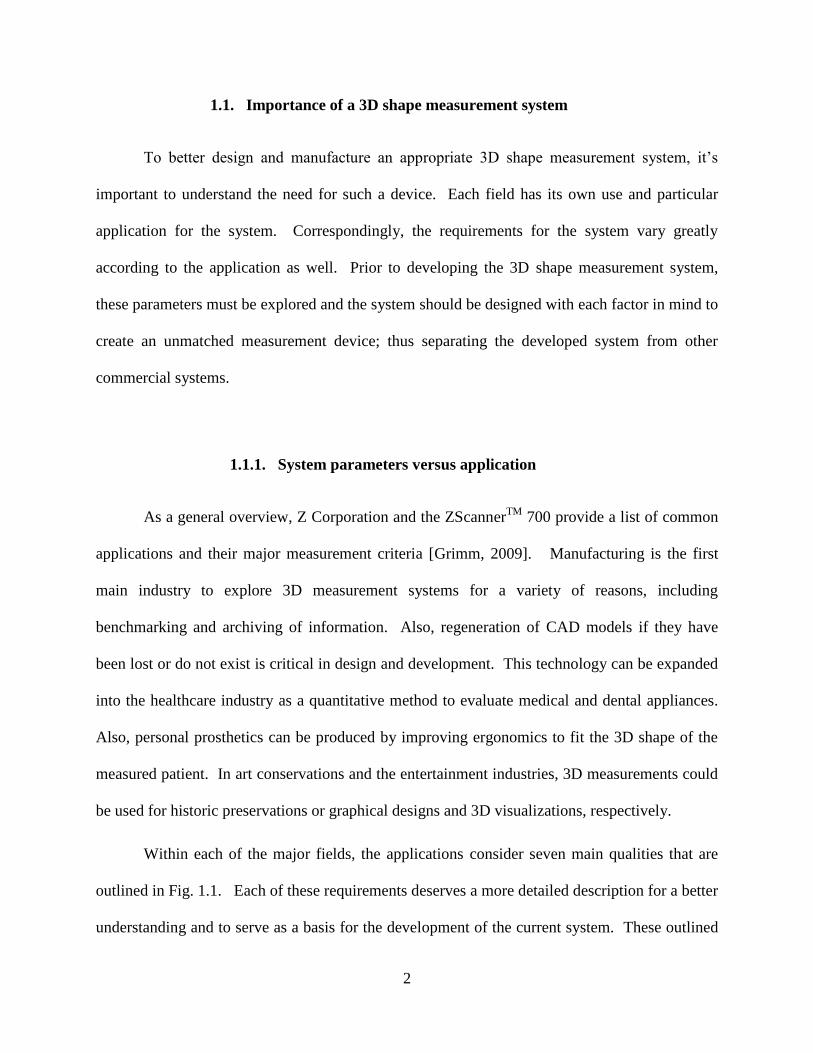
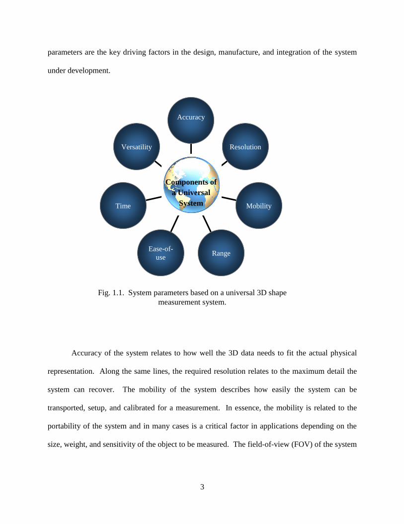
Within each of the major fields, the applications consider seven main qualities that are
outlined in Fig. 1.1. Each of these requirements deserves a more detailed description for a better
understanding and to serve as a basis for the development of the current system. These outlined
3
parameters are the key driving factors in the design, manufacture, and integration of the system
under development.
Accuracy of the system relates to how well the 3D data needs to fit the actual physical
representation. Along the same lines, the required resolution relates to the maximum detail the
system can recover. The mobility of the system describes how easily the system can be
transported, setup, and calibrated for a measurement. In essence, the mobility is related to the
portability of the system and in many cases is a critical factor in applications depending on the
size, weight, and sensitivity of the object to be measured. The field-of-view (FOV) of the system
Fig. 1.1. System parameters based on a universal 3D shape
measurement system.
Versatility
Time
Ease-of-
use Range
Mobility
Resolution
Accuracy
h Components of
a Universal
System

4
and depth of field are restrictions of the system’s range. Differing measurement techniques will
have variable range limitations.
Other factors include the measurement time once the system is set up and operational.
This is critical in some instances, such as an assembly line type of application, were components
may only have a few seconds to be scanned and benchmarked as part of the evaluation process.
Higher speeds and advanced acquisition techniques must be able to handle time limitations.
Additionally, incorporation into any commercial environment requires the system be user
friendly and easy to operate. The operator must have an understanding of how it works and the
tool must be intuitive so that measurements can be made quickly and easily. The final parameter
is versatility. The system must be versatile in terms of the number of applications, size and
complexity of the objects, and operating conditions.
Although not all of these factors are expected to be met in each and every application,
they serve as a guideline for the development. Recognizing and understanding which of these
factors is important in a particular application is critical. As an example, in benchmarking for
manufacturing, the major criteria are the versatility, accuracy, and range of the system. In
graphic design applications, the ease of use, time, and versatility are the most important
characteristics.
Current commercial systems are designed with a single application in mind. For that
reason, many consumers need to investigate current systems in detail and learn if their particular
application fits into the specification. The novel aspect of the developed system is the ability to
adopt itself to a variety of applications. In order to design an appropriate technology, an
investigation of the current techniques is required.

5
1.2. 3D shape measurement techniques
There are a variety of techniques currently existing for 3D shape measurements. For
simplification, the methodologies are separated into two main groups consisting of the contact
methods and non-contact methods. The advantages and disadvantages of each method are
described. As part of the design procedure, having an understanding of the current systems, aids
in the development of the improved device for 3D shape measurements. Additionally, the
advantages and disadvantages of each system in reference to the system requirements are
explored to better define the development specifications.
1.2.1. Contact measurements
A variety of contact systems have been developed based on varying applications. One of
the most widely used systems for 3D measurements and tolerance verification is a coordinate
measurement machine (CMM). This gives information of the x, y, z locations of an object by
using a mechanical or optical probe. CMM’s also provide information pertaining to an entire list
of characteristics defining surface features [Engineers Edge, 2011]:
Position
Parallelism/ Perpendicularity/ Angularity
Profile of a surface or line
Straightness/ Flatness/ Circularity
Cylindricity/ Symmetry/ Concentricity
Datum qualification
6
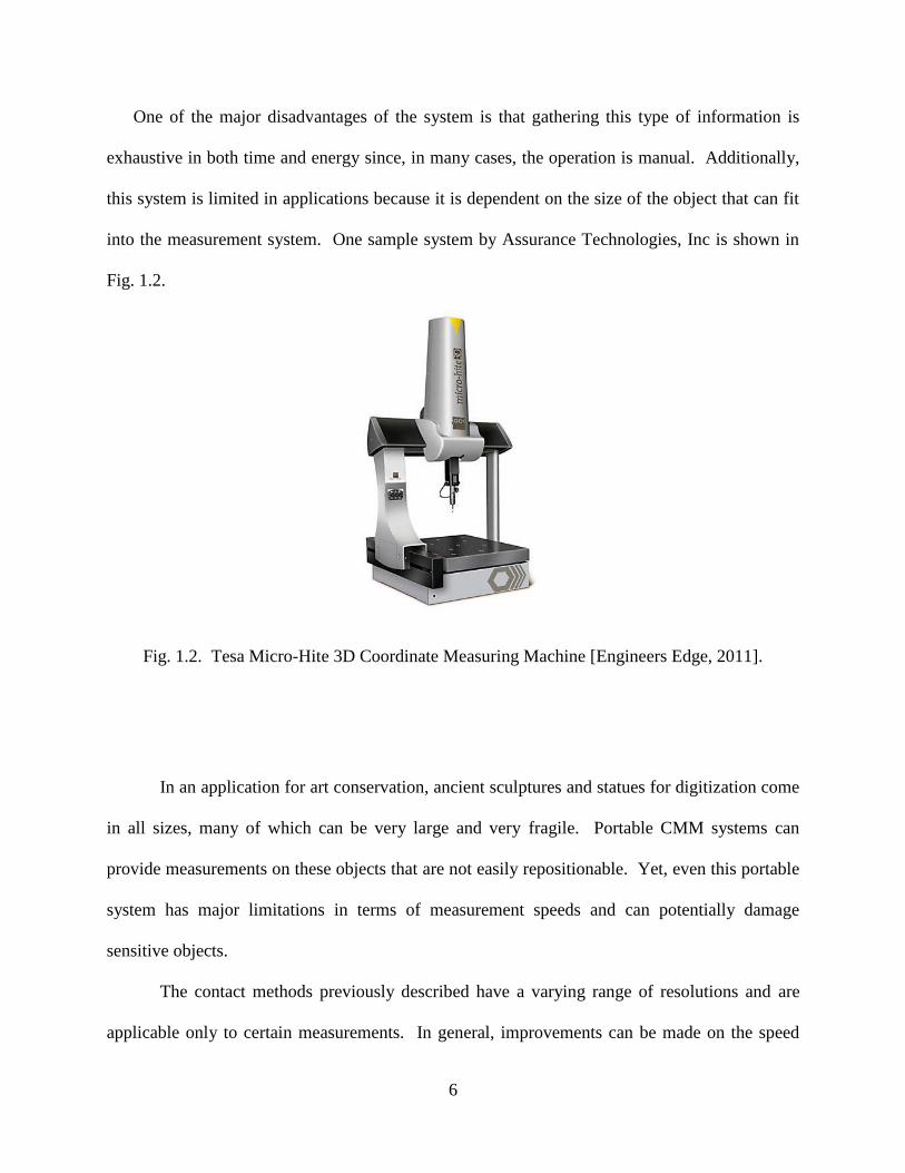
One of the major disadvantages of the system is that gathering this type of information is
exhaustive in both time and energy since, in many cases, the operation is manual. Additionally,
this system is limited in applications because it is dependent on the size of the object that can fit
into the measurement system. One sample system by Assurance Technologies, Inc is shown in
Fig. 1.2.
Fig. 1.2. Tesa Micro-Hite 3D Coordinate Measuring Machine [Engineers Edge, 2011].
In an application for art conservation, ancient sculptures and statues for digitization come
in all sizes, many of which can be very large and very fragile. Portable CMM systems can
provide measurements on these objects that are not easily repositionable. Yet, even this portable
system has major limitations in terms of measurement speeds and can potentially damage
sensitive objects.
The contact methods previously described have a varying range of resolutions and are
applicable only to certain measurements. In general, improvements can be made on the speed
7
and versatility of the 3D measurement system, while retaining the high measurement quality.
Yet, the applicability of direct contact measurements is minimal as compared to non-contact
measurements for their many advantages.
1.2.2. Non-contact measurements
Noninvasive techniques for surface measurements have become paramount for quality
analysis in industrial applications, art conservation and restoration, as well as precision aid in
medical procedures. Continued development of a structured light measurement system enhances
the versatility, applicability, and repeatability required by industry. Additionally, integration of
3D measurement techniques with computer aided design (CAD) software and computer aided
machining (CAM) equipment provides opportunities for reverse engineering [Whitehouse, 1997].
Although this technique is promising, limitations in speed and projection patterns have restricted
many systems and their potential applications.
Non-contact methods can provide many advantages over typical contact methods. First,
non-contact methods utilizing optical techniques prove to be an extremely versatile measurement
method. Within the engineering field, it has been used to solve problems in mechanics and
manufacturing technologies, while being used for nondestructive inspection [Cloud, 1998]. With
advancements in laser technology and high speed cameras with unmatched resolutions, optical
techniques provide endless opportunity in fields beyond just engineering. Other potential areas
include art conservation and forensics. The emerging strides in data acquisition and processing
provide even greater potential for these types of systems. Some of the commonly known optical
8
techniques are outlined. Required specifications that directly lead to choice of the currently
developed system are explained. Non-contact optical techniques can be classified into several
categories:
Imaging techniques
Time-of-flight techniques
Structured light techniques
1.2.2.1. Imaging techniques
Imaging techniques, classified as photogrammetry, use multiple sets of 2D images to
recover 3D information. The basic idea is that the 3D positions can be determined knowing one
corresponding location on an image. Factors that can be used to recover the shape include
shading, focus, and reflectance between images. A similar method called stereoscopy creates the
illusion of depth by simulating offset of ‘eyes’ by using two offset 2D images and the use of
special glasses to filter the images [Dodgson, 2003]. The major disadvantage of these techniques
is that 3D information is only estimated and there are difficulties in correlation of points, or
correspondence, between images. As a result, high resolution and accuracy are difficult to
achieve. Yet, the basic technology seems promising as a non-invasive, potentially high speed,
measurement system [Dornaika and Hammoudi, 2009].

9
1.2.2.2. Time-of-flight techniques
Time-of-flight techniques are based on the amount of time a laser pulse takes to get from
the system, to the object, then back to a sensor. Using simple mathematics the distances from the
system to the object can be recovered. Taking points at multiple locations the 3D information
can be used to reconstruct a CAD model of the object. Up to 100,000 points can be measured
per second and the system can be used over long distances, on the order of kilometers [Schuon et
al., 2008]. One of the disadvantages of this system is that accuracies are compromised because
the exact time-of-flight is difficult to determine. Also, errors occur when the pulse hits a point
with a large slope because the pulse is essentially averaged, arising to inaccuracies in the
measurement. Additionally, the object must remain unmoved during the point measurements, as
vibrations or motions will cause invalid reconstruction of 3D information via stitching methods.
In many applications pitch or tilt information is required, which can be determined directly using
a full field of view system, but is not easily decoded via time-of-flight measurements. Full FOV
3D measurements are difficult with this type of system.
1.2.2.3. Structured light techniques
Structured light techniques are similar to the imaging techniques previously explained.
Yet, many of the difficulties in correlation of points are eliminated by utilizing the combination
of a projection system and camera. By projecting patterns onto an object and viewing how they
deform on the object, 3D points in space can be determined via the method of triangulation from
the angle between the projector and camera. There are various methods of coding each pixel to

10
extract depth information at each point over a full field-of-view. By incorporating wave optic
techniques based on interferometry, accuracies of the system can be improved greatly. One
particular method is called fringe projection, where phase shifting is incorporated into the system
to obtain resolutions on the order of one hundredth of a wavelength.
1.3. System selection
The fringe projection – structured light technique for 3D shape measurements was chosen
for development because it offers supreme benefits over other methods for several reasons. Most
importantly, it provides high resolution results. Additionally, the FOV accommodates many
applications, on the order of mm2 to m
2. The system has the potential to be used in high speed
applications, since it can gather full FOV information in the capture of a single frame. The
incorporation of a high speed camera offers even greater potential for measurement of dynamic
scenes.
Another key feature of this technique is that it provides the greatest potential for
improvement as compared to the other techniques particularly from the projection pattern. The
development of the system must have the versatility to accommodate a variety of applications
and variations of the projection pattern or technique provides an opportunity to meet this design
criterion. The objective is to research and develop a system that can be applied to a variety of
fields because there is a great potential for 3D shape measurements in all areas. Understanding
the importance of a versatile system is critical in determining the design constraints for the
development of the system mechanically, electrically, and in regards to programming.

11
Through a clear understanding of the principle of structured light projection and the
availability of advanced technologies, a procedure has been developed to understand and utilize
the key criteria and accommodate the system based on these parameters. A detailed explanation
of how the novel system works and how it was manufactured and packaged for use in several
applications is described in forthcoming chapters.
12
2. PRINCIPLES OF STRUCTURED LIGHT PROJECTION
Structured light projection is a technique for recovering shape information as Cartesian
(x,y,z) coordinates of an object surface. By inducing a known phase shift, the measurement
precision can be improved. The most common method of structured light projection is fringe
projection. The major advantage of fringe projection over other optical techniques is to provide
full field of view information at high resolution based on the method of triangulation.
Additionally, camera video speeds are used for gathering and processing information. The fringe
projection technique has become popular in a wide range of fields and for a variety of
applications. Similar systems have been designed for the inspection of wounds, characterization
of MEMS components, and many other kinematic applications that relate to shape and position
of a moving object [Gorthi and Rastogi, 2010].
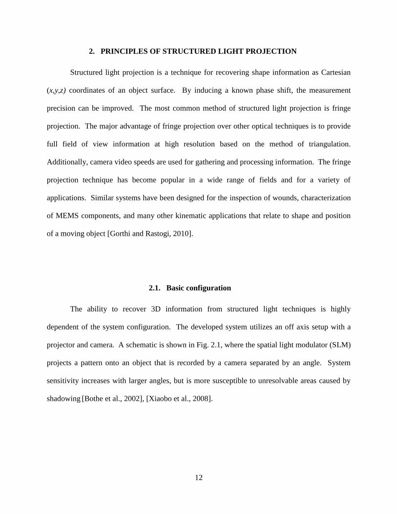
2.1. Basic configuration
The ability to recover 3D information from structured light techniques is highly
dependent of the system configuration. The developed system utilizes an off axis setup with a
projector and camera. A schematic is shown in Fig. 2.1, where the spatial light modulator (SLM)
projects a pattern onto an object that is recorded by a camera separated by an angle. System
sensitivity increases with larger angles, but is more susceptible to unresolvable areas caused by
shadowing [Bothe et al., 2002], [Xiaobo et al., 2008].

13
Triangulation is the key concept used to determine the height of the measured object,
which is directly related to the configuration of the CCD and SLM [Xiaobo, 2008]. In Fig. 2.1,
each component of the system is represented in its appropriate coordinate axis, where OP and OC
represent the origins of the projector and camera coordinate systems, respectively. The distance
from the projector to the camera, D, is known, as well as the distance from the pupil of the
projector to the reference plane, L. The camera and projector intersect at a point, M, on an
object. Knowing that triangles ΔOPMOC and ΔAMB are similar, we can write:
OP
L
Reference Plane B
A M
/
M
XP
XC ZC
ZP
Y
CCD SLM
PC
OC
X
Z D
Fig. 2.1. Schematic of fringe projection system being developed with the CCD camera
separated by a triangulation angle from the spatial light modulator (SLM).

14
The height of the object, ZM, is equivalent to the distance between the object and the
reference plane, i.e.,
It’s important to note that the reference plane is related to one of two planes – a physical
plane recorded and subtracted from the measured phase value or a mathematically removed
plane that is subtracted from the measured phase value. In either case, the relation between one
point and another in the measured data is the same. The only difference lies in the 2π
modulation that occurs from the nature of fringe projection, which introduces a mathematical
plane. The phase variation can be calculated as a function of the position shift of the projected
light ray on the reference plane [Su and Zhang, 2010]:
where the change in phase, Δφ, is the difference between the phase induced by the projection
fringes on the object, φ, and the phase induced by the projected fringes on a reference plane, φO.
fo is the spatial frequency in scaled coordinates. Solving Eq. 2.1 for AB and using the relation
from Eq. 2.2 results in AB in terms of ZM:
Based on Eq. 2.4, the solution for the value of Zm gives the height of the object of
interest:

15
where Ω is the unwrapped phase. In many cases, the distance of the system to the object, L, is
much larger than height distribution, ZM. Thus, Eq. 2.5 can be modeled as a linear relation:
A comparison between the linear and nonlinear model and its relation to calibration
techniques is analyzed by [Jia et al., 2007]. Mathematically, and by looking at Fig. 2.1, the
larger the angle, the higher the sensitivity of the system because the triangle formed from the
object to the reference is better defined. This is directly related to the accuracy of the system in
resolving the height distribution and the determination of triangle ΔAMB. A realization of the
setup in the laboratory environment is shown in Fig 2.2.
The physical setup is one component that affects the accuracy of the system. Other factors
are related to the advancements in the spatial light modulator technology and camera technology.
Additionally, defining the best projection technique is critical to recover the highest quality
Fig. 2.2. Realization of our system with an art sculpture under examination.
16
images. Research has been done on the projection technique and how it relates to image quality.
An investigation of projection techniques is critical to an understanding of how to gain the
highest quality images while still having the versatility to accommodate different applications.
2.2. Projection techniques
Different coding strategies exist in structured light projection to produce a pattern or
group of patterns that can be used to extract 3D shape information. Classifications of these
projection codes have been outlined and categorized into three major groups [Salvi et al., 2004]:
Time Multiplexing
Spatial Neighboring
Direct Coding
A basic understanding of the advantages and disadvantages of each of these methods
provides a well-rounded investigation of the chosen projection pattern as related to the objective
of the developed system. Most important is the integration of the projection pattern as related to
the advanced system components.
2.2.1. Time multiplexing
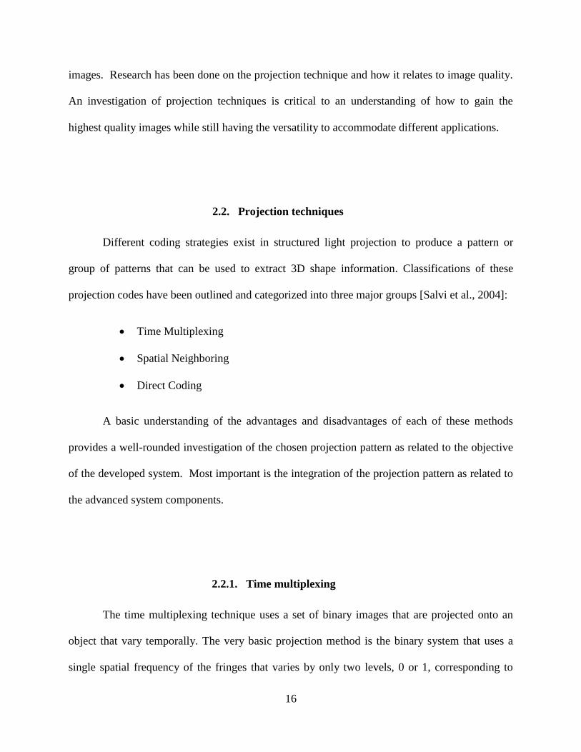
The time multiplexing technique uses a set of binary images that are projected onto an
object that vary temporally. The very basic projection method is the binary system that uses a
single spatial frequency of the fringes that varies by only two levels, 0 or 1, corresponding to
17
completely dark or completely light vertical bands, Fig. 2.3. Summation of the binary values at
each pixel level creates a binary sequence, or code word, for each particular pixel [Salvi et al.,
2004].
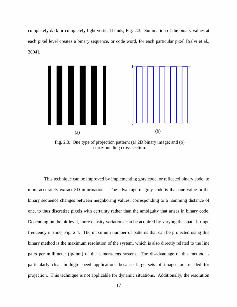
This technique can be improved by implementing gray code, or reflected binary code, to
more accurately extract 3D information. The advantage of gray code is that one value in the
binary sequence changes between neighboring values, corresponding to a hamming distance of
one, to thus discretize pixels with certainty rather than the ambiguity that arises in binary code.
Depending on the bit level, more density variations can be acquired by varying the spatial fringe
frequency in time, Fig. 2.4. The maximum number of patterns that can be projected using this
binary method is the maximum resolution of the system, which is also directly related to the line
pairs per millimeter (lp/mm) of the camera-lens system. The disadvantage of this method is
particularly clear in high speed applications because large sets of images are needed for
projection. This technique is not applicable for dynamic situations. Additionally, the resolution
Fig. 2.3. One type of projection pattern: (a) 2D binary image; and (b)
corresponding cross section.
(a) (b)
18
of the system is compromised by the resolution of the projection system and phase shifting must
be used to improve resolution. An example sequence of gray code is shown in Fig. 2.4. Hybrid
techniques include multiple pattern projects and phase shifting to improve spatial resolutions.
Fig. 2.4. Sequence of increasing density for time multiplexing technique
using binary projection patterns.
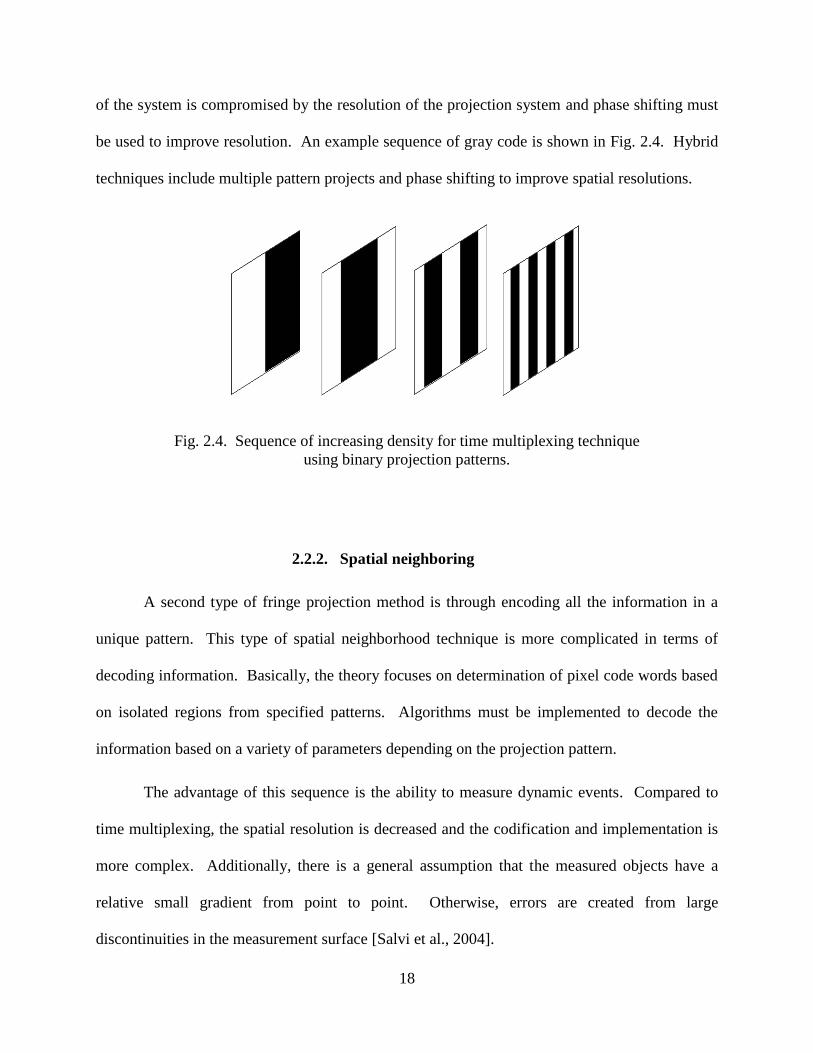
2.2.2. Spatial neighboring
A second type of fringe projection method is through encoding all the information in a
unique pattern. This type of spatial neighborhood technique is more complicated in terms of
decoding information. Basically, the theory focuses on determination of pixel code words based
on isolated regions from specified patterns. Algorithms must be implemented to decode the
information based on a variety of parameters depending on the projection pattern.
The advantage of this sequence is the ability to measure dynamic events. Compared to
time multiplexing, the spatial resolution is decreased and the codification and implementation is
more complex. Additionally, there is a general assumption that the measured objects have a
relative small gradient from point to point. Otherwise, errors are created from large
discontinuities in the measurement surface [Salvi et al., 2004].
19
2.2.3. Direct coding
The final coding method is called direct coding, where pixels can contain given
information of a certain location [Salvi et al., 2004]. One method is based on gray levels. By
modulating the pixel, the intensity can be controlled and a gray level can be achieved. This
method is highly sensitive to the stability and repeatability of the projection system for
measurements. Inaccuracies in measurements can be due to noise and non linearities in the
projection system. The main disadvantage is in the increased error when using commercial
projection systems due to quantization effects from the projector resolution and bit depth
[Xiaobo et al., 2008].
Another method is codification based on color. Using the full spectrum of RGB
information the phase map can be calculated using 24-bit color images [Spagnolo et al., 2000].
Projecting each fringe pattern individually and isolating the channels the phase map is calculated.
One factor to note is that cameras have a different absorption spectrum at different ranges of the
wavelength. These factors directly affect the phase map, particularly when examining each color
channel. Some methods use a combination of three-phase step contained in a single frame
isolated by red, green, and blue fringes. Post-processing can be done to isolate each channel and
perform the three-phase step algorithm. One of the major drawbacks of this method was directly
related to the large bandwidth associated with the use of LCD projection systems that cause
ambiguity among intensity values between pixels. Additionally, the effects of noise from the
system play a large role in the applicability of this technique.
20
2.3. Fringe projection system
Based on the analysis of different structured light projection techniques, the method of
direct coding provides the best resolution and accuracy along with high speeds. This technique
has the potential to combine phase shifting for improved results and the versatility to
accommodate high speed applications. Incorporation of this method into the development of the
system requires an understanding of the mathematics behind fringe projection.
For fringe projection, sinusoidal patterns are critical because they minimize
discontinuities and errors in the reconstruction algorithms. This project explores the
mathematical importance of sinusoidal projections while analyzing their quality via
quantification of processed images, which will help in the continued development of our system
as a combined high-speed, high resolution versatile measurement device. From a mathematical
standpoint, a 1D Fourier approximation, f(x), contains only the summation of continuous cosine
and sine approximations, with integration functions, an and bn, discontinuities will appear as high
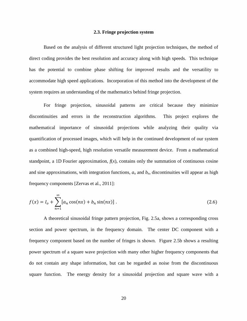
frequency components [Zervas et al., 2011]:
∑[ ]
A theoretical sinusoidal fringe pattern projection, Fig. 2.5a, shows a corresponding cross
section and power spectrum, in the frequency domain. The center DC component with a
frequency component based on the number of fringes is shown. Figure 2.5b shows a resulting
power spectrum of a square wave projection with many other higher frequency components that
do not contain any shape information, but can be regarded as noise from the discontinuous
square function. The energy density for a sinusoidal projection and square wave with a
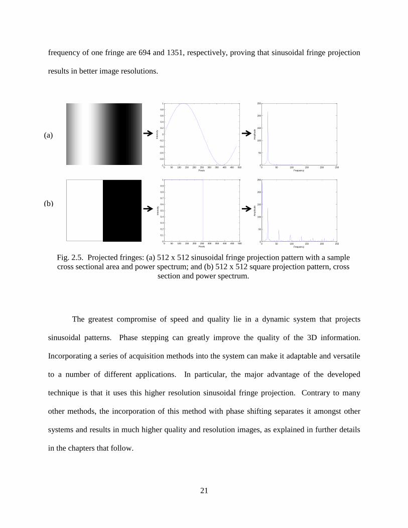
21
frequency of one fringe are 694 and 1351, respectively, proving that sinusoidal fringe projection
results in better image resolutions.
The greatest compromise of speed and quality lie in a dynamic system that projects
sinusoidal patterns. Phase stepping can greatly improve the quality of the 3D information.
Incorporating a series of acquisition methods into the system can make it adaptable and versatile
to a number of different applications. In particular, the major advantage of the developed
technique is that it uses this higher resolution sinusoidal fringe projection. Contrary to many
other methods, the incorporation of this method with phase shifting separates it amongst other
systems and results in much higher quality and resolution images, as explained in further details
in the chapters that follow.
(a)
(b)
0 50 100 150 200 250 300 350 400 450 500-1
-0.8
-0.6
-0.4
-0.2
0
0.2
0.4
0.6
0.8
1
Pixels
Inte
nsity
0 50 100 150 200 250 300 350 400 450 5000
0.1
0.2
0.3
0.4
0.5
0.6
0.7
0.8
0.9
1
Pixels
Inte
nsity
0 50 100 150 200 2500
50
100
150
200
250
Frequency
Am
plitu
de
0 50 100 150 200 2500
50
100
150
200
250
Frequency
Am
plitu
de
Fig. 2.5. Projected fringes: (a) 512 x 512 sinusoidal fringe projection pattern with a sample
cross sectional area and power spectrum; and (b) 512 x 512 square projection pattern, cross
section and power spectrum.
22
3. OPTICAL PHASE CALCULATION AND UNWRAPPING
An understanding of the basic system configuration is an initial step in the development
of the 3D shape measurement system. A more detailed understanding of the acquisition and
unwrapping processes for recovering 3D information is required. To gather information in
versatile conditions, at high speeds and high resolutions, different algorithms must be
implemented. An understanding of signal processing is essential for maximizing image quality.
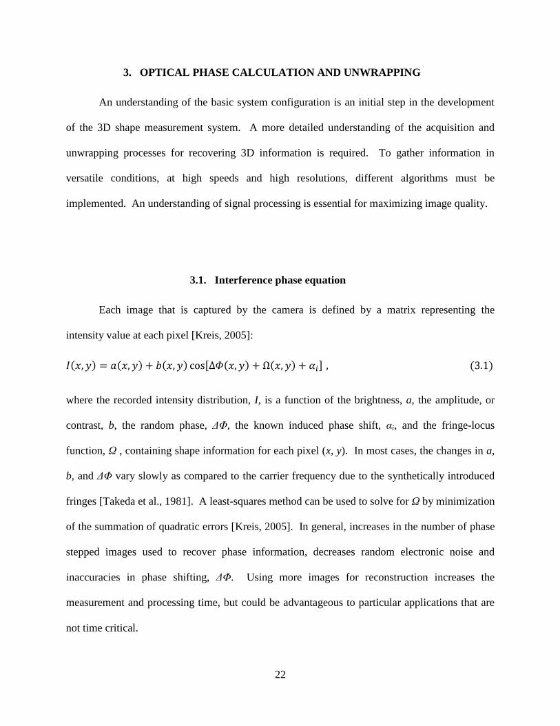
3.1. Interference phase equation
Each image that is captured by the camera is defined by a matrix representing the
intensity value at each pixel [Kreis, 2005]:
[ ]
where the recorded intensity distribution, I, is a function of the brightness, a, the amplitude, or
contrast, b, the random phase, ΔΦ, the known induced phase shift, αi, and the fringe-locus
function, Ω , containing shape information for each pixel (x, y). In most cases, the changes in a,
b, and ΔΦ vary slowly as compared to the carrier frequency due to the synthetically introduced
fringes [Takeda et al., 1981]. A least-squares method can be used to solve for Ω by minimization
of the summation of quadratic errors [Kreis, 2005]. In general, increases in the number of phase
stepped images used to recover phase information, decreases random electronic noise and
inaccuracies in phase shifting, ΔΦ. Using more images for reconstruction increases the
measurement and processing time, but could be advantageous to particular applications that are
not time critical.

23
3.2. Fast-Fourier Transform (FFT) single frame phase calculation
For high speed applications, single images must be used to recover 3D information. A
Fast-Fourier Transform (FFT) evaluation is one technique for acquiring phase information via a
single image. Processing is done on a captured image with sinusoidal fringes projected onto the
object of interest. The density of the fringes is chosen based on the FOV and desired resolution.
The FFT essentially fits a sequence of harmonic spatial functions with increasing frequency to
the acquired image, which converts the data from the time domain into the frequency domain.
The basis behind the theory is that a signal can be decomposed into a series of its sine and cosine
functions.
Mathematically, the Fourier Transformation, F(u), can be written in terms of the amount
of each frequency that makes f(x). The important characteristic of the Fourier Transform is that
the spatial signal can be recovered by an inverse transformation:
∫
∫
This phenomenon can be applied to a single image by utilizing Euler’s identity shown in Eq. 3.4
to simplify Eq. 3.1:
Thus, Eq. 3.1 is rearranged for convenience into Eq. 3.5 and extended into 2D for image
analysis.

24
where
The complex conjugate is represented as c*
in Eq. 3.5. Applying a 2D FFT to the image
results in the direct representation of the DC component, a(u,v) and the spatial frequency, c(u,v)
and c*(u,v), Eq. 3.5. The information is now transformed into the frequency domain where it can
be viewed as a function of the amplitude, also known as the power spectrum, Eq. 3.7.
√ ( )
Based on the Nyquist Sampling Theory, the summation is performed on half of the image
pixel dimension, but the result is a complex number which means the total number of terms is the
same as the input image size. The power spectrum, or magnitude, is the combined amplitude of
the summations of sine and cosine functions. Since the analysis is done on a real signal, the FFT
matrix is point symmetric with respect to the DC term at I(0,0) [Kreis, 2005]. A sample FFT is
shown in Fig. 3.1 with high density fringes on a sculpture. For viewing and filtering purposes, a
logarithmic scale showing only the real components are plotted. Also, the zero-frequency
component was shifted to the center of the image by shifting quadrants.
25
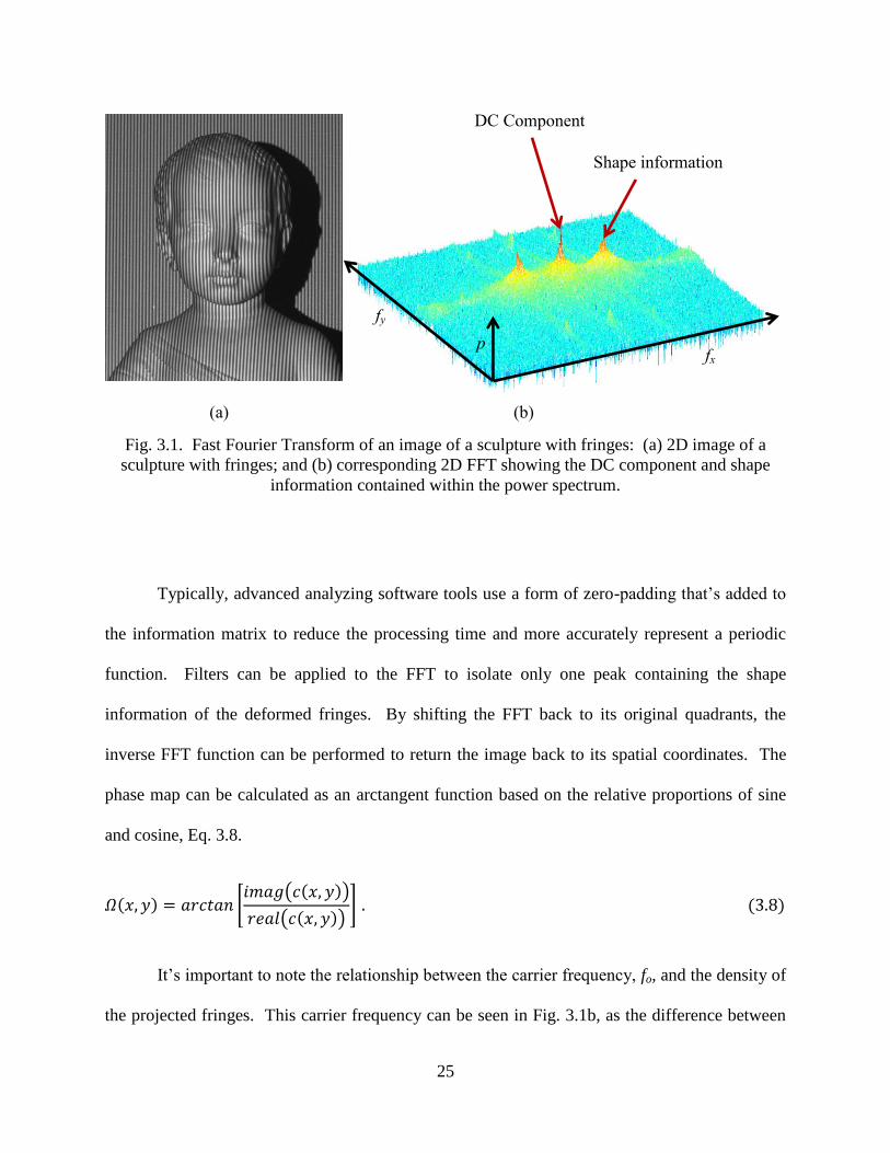
Fig. 3.1. Fast Fourier Transform of an image of a sculpture with fringes: (a) 2D image of a
sculpture with fringes; and (b) corresponding 2D FFT showing the DC component and shape
information contained within the power spectrum.
Typically, advanced analyzing software tools use a form of zero-padding that’s added to
the information matrix to reduce the processing time and more accurately represent a periodic
function. Filters can be applied to the FFT to isolate only one peak containing the shape
information of the deformed fringes. By shifting the FFT back to its original quadrants, the
inverse FFT function can be performed to return the image back to its spatial coordinates. The
phase map can be calculated as an arctangent function based on the relative proportions of sine
and cosine, Eq. 3.8.
[ ( )
( )]
It’s important to note the relationship between the carrier frequency, fo, and the density of
the projected fringes. This carrier frequency can be seen in Fig. 3.1b, as the difference between
DC Component
Shape information
fx
fy
p
(a) (b)
26
the frequency values of the DC component peak and shape information peak. Theoretically, the
broader the fringe density, the lower order of the term that is needed to represent the fringe
frequency and the closer the peak will be to the central DC component. The larger the fringe
frequency, the higher order of the term that represents the fringes and the further away from the
central DC component it will be, thus resulting in a larger carrier frequency. The resulting
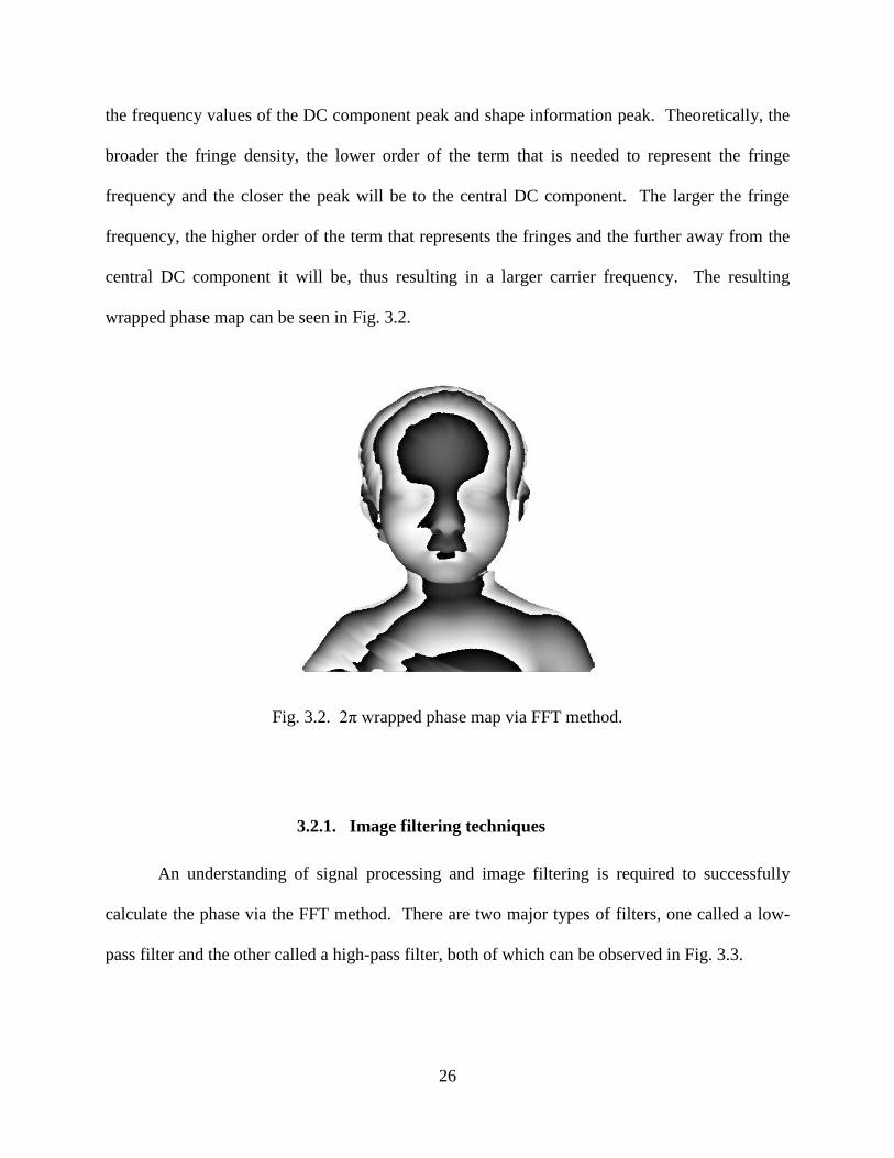
wrapped phase map can be seen in Fig. 3.2.
Fig. 3.2. 2π wrapped phase map via FFT method.
3.2.1. Image filtering techniques
An understanding of signal processing and image filtering is required to successfully
calculate the phase via the FFT method. There are two major types of filters, one called a low-
pass filter and the other called a high-pass filter, both of which can be observed in Fig. 3.3.

27
Fig. 3.3. Frequency domain filters: (a) Butterworth Low Pass Filter; and (b) Butterworth High
Pass Filter.
The low-pass filter is also known as a smoothing frequency filter. For image processing,
a Butterworth Low-Pass Filter (BLPF) was used of order n with a cutoff frequency at distance Do
from the center, Eq. 3.9 [Gonzales et al., 2009]:
[ ]
where H(u,v) is the filter transform function. A customary function for D(u,v) based on a
Euclidian distance function was formed from the matrix size of the input image. Each element
value is the Euclidian distance to the nearest corner. Converse to the BLPF, the Butterworth
High-Pass Filter (BHPF) is used for ‘sharpening’ images by eliminating the low frequencies and
retaining only the high frequency components.
[ ]
(a) (b)

28
Several notes should be made about these filters. First, they do not contain any sharp
discontinuities at Do which eliminates any source of high frequency noise once the phase map is
recovered. Also, these filters are applied to the shifted FFT spectrum, where the low frequency
components are directly shifted to the origin. The filter transform functions can be directly
multiplied by the FFT spectrum, such that the following applies:
⇔
where is the convolution of two functions. Convolution in the spatial domain is equivalent to
the direct matrix multiplication in the frequency domain. The reverse also exists, but we only
consider the first phenomenon in Eq. 3.11 because filtering and phase calculation is critically
dependent on frequency domain analysis. The ⇔ symbol represents a Fourier Transform pair
[Gonzales et al., 2009]. Appendix A shows the FFT method implemented into MatLab.
In order to isolate the fringe locus function, two of the major types of filters, shown in
Fig. 3.4, were experimented, where black represents a value of zero and white a value of one.
The edges of the filter are padded to reduce high frequency noise in the final phase map. A
balance exists between the size of the filter and quality of the image. The high frequency
contained in the FFT improves the ‘sharpness’ of the wrapped phase map between boundaries. If
the filter is too narrow and only isolates directly the shape information, the quality of the image
is degraded.

29
Fig. 3.4. Frequency domain filters applied to images: (a) BLPF; and (b) zero padded square
filter.
Several critical factors affect the ability to recover phase in the frequency domain and
applicability of each filter. First is the relationship between the fringe density and the DC
component. The high amplitude peaks associated with fringes have to be sufficiently separated
from the DC component, Fig. 3.5, for the best filtering and phase results. Otherwise, there is
overlapping of information that cannot be separated using the filters. The extent of the DC is
also directly proportional to the variability in the reflectivity of the object.
Figure 3.5 shows two fringe frequencies and the corresponding shape information
contained in the highest amplitude peaks offset from the center DC component. Figure 3.5a is of
a high density, 4 pixels per fringe. Aliasing can be seen from the high amplitude peaks at higher
frequencies. Figure 3.5b shows lower density fringe, 16 pixels per fringe, with high amplitude
peaks located significantly closer to the DC component.
100 200 300 400 500 600 700 800 900 1000
100
200
300
400
500
600
700
800
900
1000 100 200 300 400 500 600 700 800 900 1000
100
200
300
400
500
600
700
800
900
1000
(a) (b)

30
Fig. 3.5. FFT of two different fringe densities across a flat reference surface: (a) high density
projection of 4 pixels per fringe; and (b) low density projection at 16 pixels per fringe.
In terms of the filters, when there is other high-frequency noise in the images from
aliasing affects as those seen Fig. 3.5a, a BLPF can be used to isolate only the shape information
over a narrow area to produce a high quality phase map. Conversely, if there is little aliasing
effects then the square filter could be used to incorporate more high frequency components for a
sharper result.
3.3. Phase Shifting Method (PSM) of interferometry
In high resolution applications where measurement accuracy is paramount, considerations
have to be placed on the method of phase determination. Phase stepping provides an advantage
of directly recovering the three unknown variable of brightness, contrast, and phase in the
intensity equation by introducing a known shift. By using at least 3 phase stepped images, a
phase map can be resolved. Unlike most other phase stepping applications, the developed
14 bit 4 p/f
frequency
frequency
100 200 300 400 500 600
50
100
150
200
250
300
350
400
450 6
8
10
12
14
16
18
20
14 bit 16 p/f
frequency
frequency
100 200 300 400 500 600
50
100
150
200
250
300
350
400
4505
10
15
20
(a) (b)
31
system is nearly insensitive to phase shifting calibration due to precision control of the projection
pattern that is explained in greater details in chapter 4.
One general method for determination of the phase value via phase shifting is the
Gaussian least squares approach. The simplified basic intensity equation as a function of (x,y)
pixel location, the fringe locus function and phase shift is:
[ ]
Equation 3.12 can be transformed based on the following trigonometric identity using the
summations of two variables within a cosine function.
Utilizing the identity of Eq. 3.13, the value of the cosine function in Eq. 3.12 can be revised to
form the following results:
[ ] [ ]
For simplification the values of u and v are set to the following:
[ ]
[ ]
Thus, the intensity equation can be simplified by substituting Eqs. 3.15 and 3.16 into Eq. 3.14.
The pixel positions (x,y) are omitted for clarity:

32
where n is the image number. Summation of the quadratic errors needs to be minimized by
setting the equation to zero and partially differentiating with respect to each of the three
variables. The results are a system of three equations with three unknowns that can be
summarized by the matrix shown in Eq. 3.18, with the full solution in Appendix B.
[ ∑ ∑
∑ ∑ ∑
∑ ∑ ∑ ]
[ ]
[ ∑
∑
∑ ]
Noting that the value of the wrapped phase is equal to:
[
]
The system of equations in Eq. 3.18 can be solved for an arbitrary number of phase stepped
images, resulting in the wrapped phase:
∑ [ ]
∑ [ ]
where α is the value of the phase shift in degrees. With an arbitrary number of shifts, the phase
can be calculated. The algorithm is implemented for 4, 8, and 16 phase steps using MatLab and
shown in Appendix C.
33
3.4. The unwrapping problem
Processing and viewing the information at varying speeds requires an unwrapping
algorithm. The shape information contained in the phase map of the data is wrapped within an
upper and lower boundary of π to – π due to the arctangent function in the mathematics of the
phase calculations [Ghiglia and Pritt, 1998]. When an upper or lower boundary is achieved, a
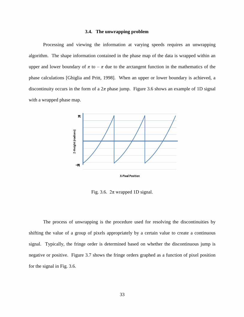
discontinuity occurs in the form of a 2π phase jump. Figure 3.6 shows an example of 1D signal
with a wrapped phase map.
Fig. 3.6. 2π wrapped 1D signal.
The process of unwrapping is the procedure used for resolving the discontinuities by
shifting the value of a group of pixels appropriately by a certain value to create a continuous
signal. Typically, the fringe order is determined based on whether the discontinuous jump is
negative or positive. Figure 3.7 shows the fringe orders graphed as a function of pixel position
for the signal in Fig. 3.6.
-π
π
34
5π
-π
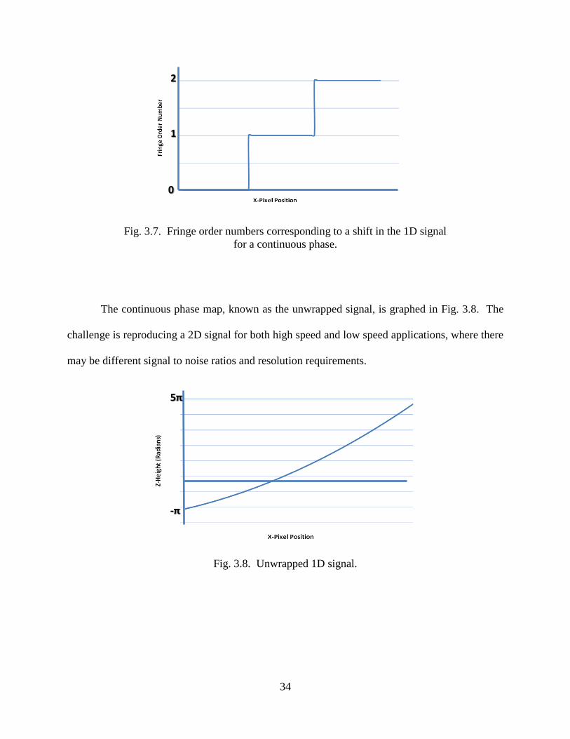
Fig. 3.7. Fringe order numbers corresponding to a shift in the 1D signal
for a continuous phase.
The continuous phase map, known as the unwrapped signal, is graphed in Fig. 3.8. The
challenge is reproducing a 2D signal for both high speed and low speed applications, where there
may be different signal to noise ratios and resolution requirements.
Fig. 3.8. Unwrapped 1D signal.
0
1
2
35
Understanding of the basic unwrapping problems aids in an understanding of the
advantages and disadvantages of other unwrapping algorithms. The key feature is utilizing the
appropriate unwrapping algorithms based on the particular requirements of the application.
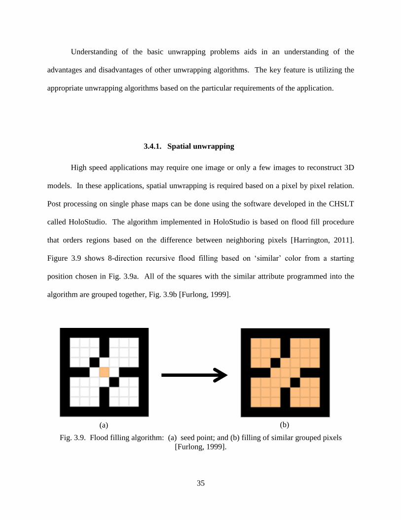
3.4.1. Spatial unwrapping
High speed applications may require one image or only a few images to reconstruct 3D
models. In these applications, spatial unwrapping is required based on a pixel by pixel relation.
Post processing on single phase maps can be done using the software developed in the CHSLT
called HoloStudio. The algorithm implemented in HoloStudio is based on flood fill procedure
that orders regions based on the difference between neighboring pixels [Harrington, 2011].
Figure 3.9 shows 8-direction recursive flood filling based on ‘similar’ color from a starting
position chosen in Fig. 3.9a. All of the squares with the similar attribute programmed into the
algorithm are grouped together, Fig. 3.9b [Furlong, 1999].
Fig. 3.9. Flood filling algorithm: (a) seed point; and (b) filling of similar grouped pixels
[Furlong, 1999].
(a) (b)

36
The algorithm is completed using four sequential steps with four parameters that include
the seeding point, group size, threshold, and extent. The algorithm begins by first picking a
starting point, or pixel p, which is called the seeding point, similar to the starting point shown in
Fig. 3.9a. From this point, the algorithm works outwards by adding neighboring pixels, p’, to
create one group for all pixels contained by the threshold, t, in radians based on the relation in
Eq. 3.20:
| |
Once no more pixels can be added to the group, the algorithm determines if the group is
smaller or larger than the minimum group size, g. If the group is smaller than g then the group is
discarded and those pixels are marked as null [Harrington et al., 2011]. Starting again at an
alternate seeding point, the proceeding steps are repeated until all pixels are assigned to a group
or discarded. The difference between pixels of neighboring groups is recorded. The first group
with its seeding point, is assigned a level of N=0 representing no modification to its values.
Next, each group is examined sequentially to find the longest border with a neighbor. That
neighbor is assigned a value of N relative to the group that is known. This is done by using the
value of the difference between two neighboring groups and using relation in Eq. 3.21:
If the group is less than π, then the value of the new group is assigned a value N one less
than the reference group. The opposite is true for neighboring groups that have a value greater
than π, in which case the group is then assigned a value N greater than the reference group. The
final step is reassignment of the value of the pixels, Eq. 3.22, by the addition of 2π multiplied by
the group value, N:

37
The developed algorithm for spatial unwrapping runs approximately 10-50 times faster
than the previous spatial unwrapping algorithm [Harrington et al., 2011]. Speed is critical in
processing of large sets of data, particularly for high speed applications. The effectiveness of the
algorithm depends directly on the quality of phase map and the signal to noise ratio in the image.
3.4.2. Temporal phase unwrapping
Spatial unwrapping techniques have drawbacks from discontinuous neighboring pixels on
the surface profile that create and propagate errors in the 2π unwrapping [Huntley and Saldner,
1997]. Thus, temporal unwrapping is another algorithm for resolving discontinuities in the
wrapped phase map of an image. Unlike 2D spatial unwrapping, temporal unwrapping is
executed in 1D along the time axis, using differing fringe densities. Consequently, pixels are not
affected by poor signal to noise ratios in neighboring pixels, reducing errors seen in spatial
unwrapping [Kinell, 2000]. This approach is also called a hierarchical technique, by varying the
fringe period, P, from the largest period to the smallest period, the temporal unwrapping
algorithm can be implemented. The broadest fringe density, K, should have no 0-2π
discontinuities, Fig. 3.10.
38
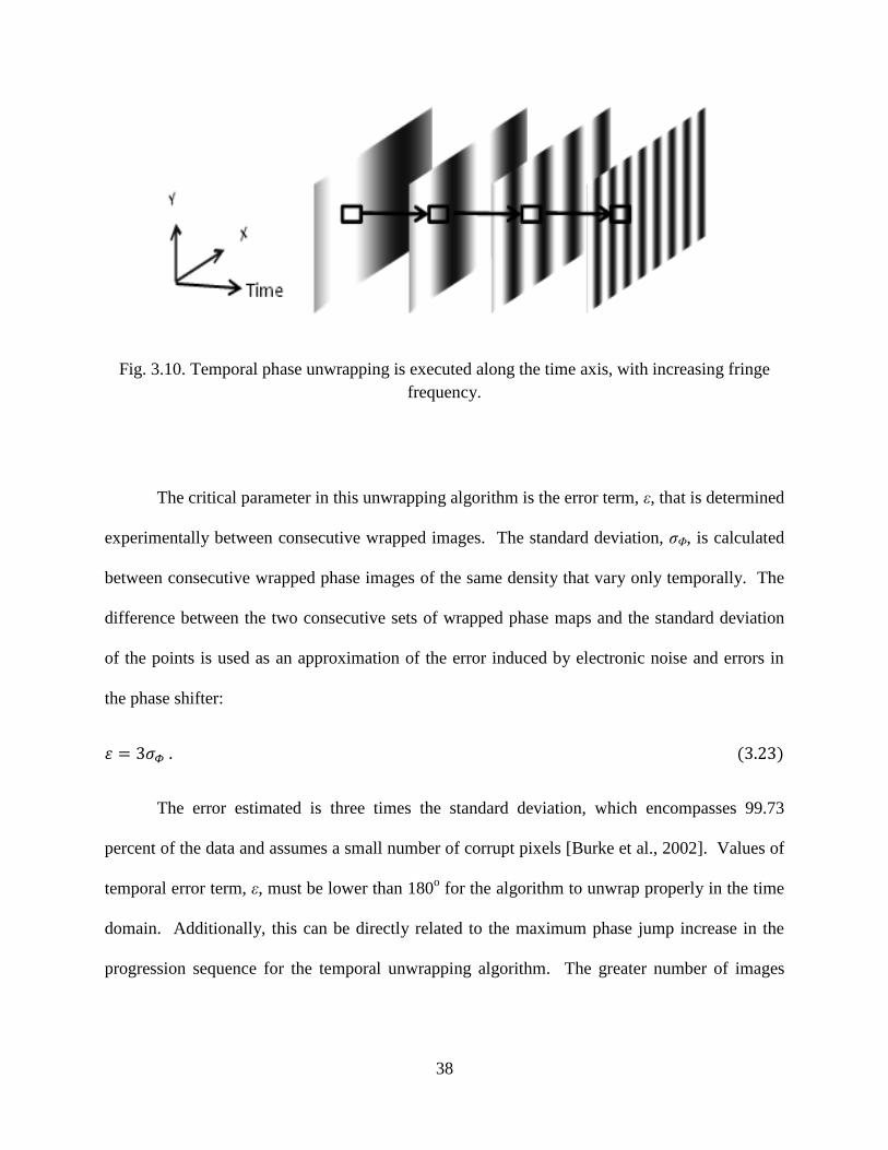
Fig. 3.10. Temporal phase unwrapping is executed along the time axis, with increasing fringe
frequency.
The critical parameter in this unwrapping algorithm is the error term, ε, that is determined
experimentally between consecutive wrapped images. The standard deviation, σΦ, is calculated
between consecutive wrapped phase images of the same density that vary only temporally. The
difference between the two consecutive sets of wrapped phase maps and the standard deviation
of the points is used as an approximation of the error induced by electronic noise and errors in
the phase shifter:
The error estimated is three times the standard deviation, which encompasses 99.73
percent of the data and assumes a small number of corrupt pixels [Burke et al., 2002]. Values of
temporal error term, ε, must be lower than 180o for the algorithm to unwrap properly in the time
domain. Additionally, this can be directly related to the maximum phase jump increase in the
progression sequence for the temporal unwrapping algorithm. The greater number of images
39
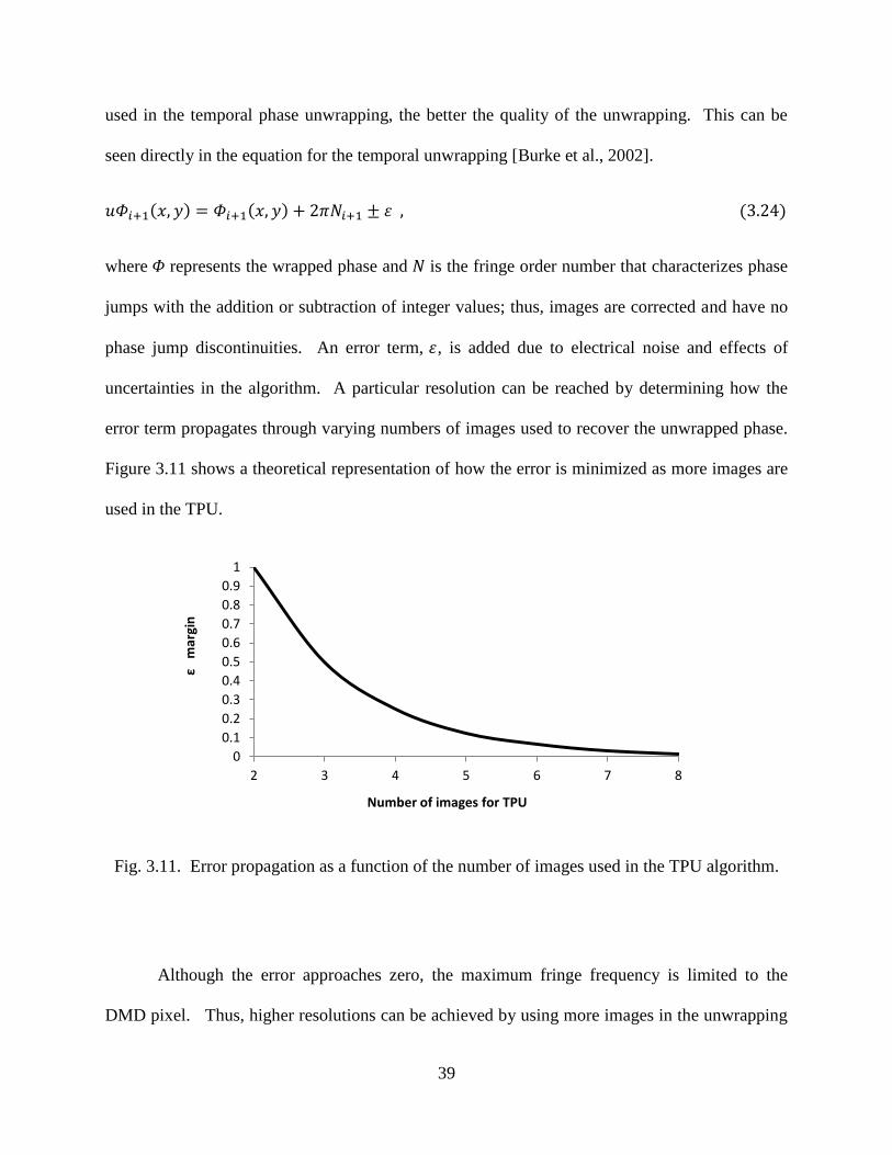
used in the temporal phase unwrapping, the better the quality of the unwrapping. This can be
seen directly in the equation for the temporal unwrapping [Burke et al., 2002].
where represents the wrapped phase and is the fringe order number that characterizes phase
jumps with the addition or subtraction of integer values; thus, images are corrected and have no
phase jump discontinuities. An error term, , is added due to electrical noise and effects of
uncertainties in the algorithm. A particular resolution can be reached by determining how the
error term propagates through varying numbers of images used to recover the unwrapped phase.
Figure 3.11 shows a theoretical representation of how the error is minimized as more images are
used in the TPU.
Fig. 3.11. Error propagation as a function of the number of images used in the TPU algorithm.
Although the error approaches zero, the maximum fringe frequency is limited to the
DMD pixel. Thus, higher resolutions can be achieved by using more images in the unwrapping
0
0.1
0.2
0.3
0.4
0.5
0.6
0.7
0.8
0.9
1
2 3 4 5 6 7 8
ε m
argi
n
Number of images for TPU
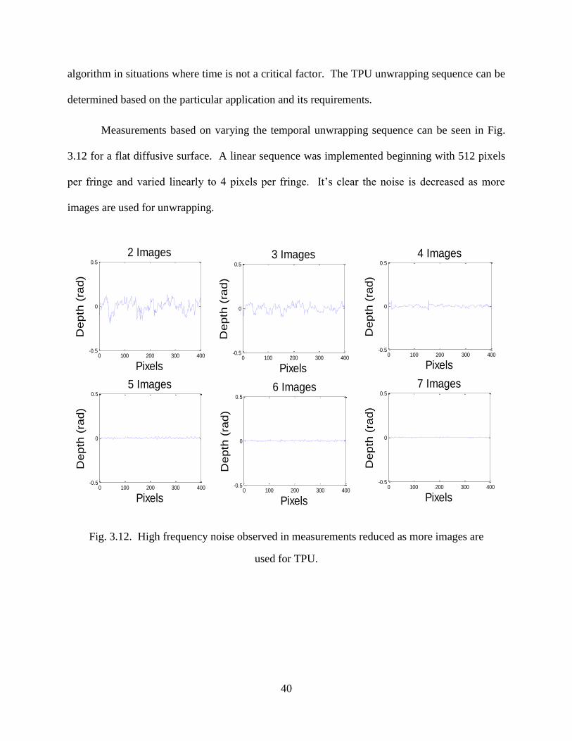
40
algorithm in situations where time is not a critical factor. The TPU unwrapping sequence can be
determined based on the particular application and its requirements.
Measurements based on varying the temporal unwrapping sequence can be seen in Fig.
3.12 for a flat diffusive surface. A linear sequence was implemented beginning with 512 pixels
per fringe and varied linearly to 4 pixels per fringe. It’s clear the noise is decreased as more
images are used for unwrapping.
Fig. 3.12. High frequency noise observed in measurements reduced as more images are
used for TPU.
0 100 200 300 400-0.5
0
0.5
Pixels
Depth
(ra
d)
7 Images
0 100 200 300 400-0.5
0
0.5
Pixels
Depth
(ra
d)
6 Images
0 100 200 300 400-0.5
0
0.5
Pixels
Depth
(ra
d)
5 Images
0 100 200 300 400-0.5
0
0.5
Pixels
Depth
(ra
d)
4 Images
0 100 200 300 400-0.5
0
0.5
Pixels
Depth
(ra
d)
3 Images
0 100 200 300 400-0.5
0
0.5
Pixels
Depth
(ra
d)
2 Images
0 100 200 300 400-0.5
0
0.5
Pixels
Depth
(ra
d)
7 Images
0 100 200 300 400-0.5
0
0.5
Pixels
Depth
(ra
d)
6 Images
0 100 200 300 400-0.5
0
0.5
Pixels
Depth
(ra
d)
5 Images
0 100 200 300 400-0.5
0
0.5
Pixels
Depth
(ra
d)
4 Images
0 100 200 300 400-0.5
0
0.5
Pixels
Depth
(ra
d)
3 Images
0 100 200 300 400-0.5
0
0.5
PixelsD
epth
(ra
d)
2 Images
0 100 200 300 400-0.5
0
0.5
Pixels
Depth
(ra
d)
7 Images
0 100 200 300 400-0.5
0
0.5
Pixels
Depth
(ra
d)
6 Images
0 100 200 300 400-0.5
0
0.5
Pixels
Depth
(ra
d)
5 Images
0 100 200 300 400-0.5
0
0.5
PixelsD
epth
(ra
d)
4 Images
0 100 200 300 400-0.5
0
0.5
Pixels
Depth
(ra
d)
3 Images
0 100 200 300 400-0.5
0
0.5
Pixels
Depth
(ra
d)
2 Images
0 100 200 300 400-0.5
0
0.5
Pixels
Depth
(ra
d)
7 Images
0 100 200 300 400-0.5
0
0.5
Pixels
Depth
(ra
d)
6 Images
0 100 200 300 400-0.5
0
0.5
Pixels
Depth
(ra
d)
5 Images
0 100 200 300 400-0.5
0
0.5
Pixels
Depth
(ra
d)
4 Images
0 100 200 300 400-0.5
0
0.5
Pixels
Depth
(ra
d)
3 Images
0 100 200 300 400-0.5
0
0.5
Pixels
Depth
(ra
d)
2 Images
0 100 200 300 400-0.5
0
0.5
Pixels
Depth
(ra
d)
7 Images
0 100 200 300 400-0.5
0
0.5
PixelsD
epth
(ra
d)
6 Images
0 100 200 300 400-0.5
0
0.5
Pixels
Depth
(ra
d)
5 Images
0 100 200 300 400-0.5
0
0.5
Pixels
Depth
(ra
d)
4 Images
0 100 200 300 400-0.5
0
0.5
Pixels
Depth
(ra
d)
3 Images
0 100 200 300 400-0.5
0
0.5
PixelsD
epth
(ra
d)
2 Images

41
A linear progression of increased fringe frequency was tested against an exponential
sequence. Figure 3.13 shows the progression sequence as a function and the standard deviation
between data points starting from the minimum number of images and increasing.
Fig. 3.13. Minimization of errors as function of number of images used in TPU for linear and
exponential sequences.
Based on the results, the error is minimized faster when using the exponential sequence,
but the major limitation is the number of images used for the unwrapping. The exponential
sequence can use a maximum of 4 images corresponding to 512, 256, 64, and 4 pixels per fringe,
which is the maximum range of our system.
0
0.01
0.02
0.03
0.04
0.05
0.06
0.07
2 3 4 5 6 7 8
Std
De
viat
ion
Number of Images Used for TPU
Linear Sequence
Exponential Sequence
42
4. SYSTEM DEVELOPMENT AND ANALYSIS
The Fringe Projection system consists of two major components, a spatial light modulator
(SLM) and a digital charged-couple device (CCD) camera. Varying parameters, such as
exposure time, fringe density, and field of view, affect the system’s resolutions and image
quality. Yet, these factors are heavily dependent on the application requirements and object of
interest. Based on the first generation prototype, evaluations on the basic effects of varying
differing exposures, the quality of the sinusoidal projected patterns, and the effects of varying the
CCD and SLM configuration were explored.
4.1. System design
The development and design of the fringe projection system for 3D shape measurements
is based on advanced technologies achieved through sophisticated integration of a SLM with a
CCD camera. The SLM, packaged by Vialux, contains a digital light processing (DLP®) unit
from Texas Instruments called DLP Discovery™ [Texas Instruments, 2010a]. Utilizing the
functionality of a field-programmable gate array (FPGA) integrated circuit, the fringe projection
system was customized for high speed, sinusoidal fringe projection. The major advantage of this
circuit is the ability to directly configure and reconfigure to accommodate a variety of projection
patterns based on a particular application.

43
4.2. MEMS based system improvements
The system uses a Digital Micro-mirror Device (DMD) with a 1080 x 1920 chip
resolution that enables sinusoidal fringe projection [Texas Instruments, 2010a]. Based on
previous research, this particular system is idealized for the use of gray scale sinusoidal
projection because of direct control of each micro mirror. The system has high precision,
repeatable achieved by controlling each of the mirrors, or pixels, in the DMD, Fig. 4.1.
The system, created by Texas Instruments and shown in Appendix D, works by direct
control of the mirror’s position, which can be in one of two states - on or off. The center of each
10x10 µm2 device is held by a support post and controlled precisely by a MEMS based
component. The mirrors are made to rotate at an angle of ±10 degrees that depend on the binary
state of the cell below the mirror, Fig 4.2. When a particular voltage is applied to the electrode
below a mirror, an electro-static force is created that positions the mirror in a particular
Fig. 4.1. Device developed by Texas Instruments and used in our fringe projection
system: (a) DMD chip; and (b) Enlarged view of micro mirrors enabling
sinusoidal projection [Texas Instruments, 2010b].
20
m
Number of mirrors 1080 x 1920
(a) (b)
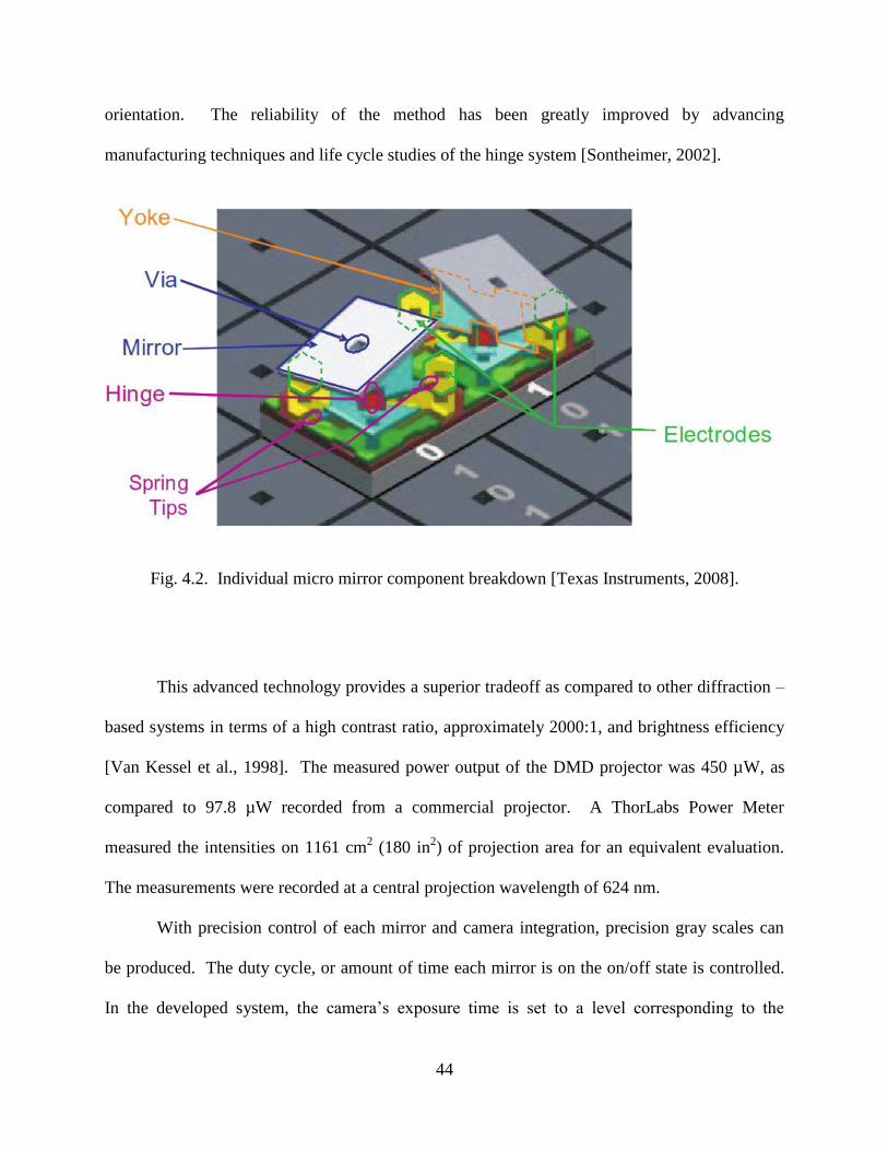
44
orientation. The reliability of the method has been greatly improved by advancing
manufacturing techniques and life cycle studies of the hinge system [Sontheimer, 2002].
Fig. 4.2. Individual micro mirror component breakdown [Texas Instruments, 2008].
This advanced technology provides a superior tradeoff as compared to other diffraction –
based systems in terms of a high contrast ratio, approximately 2000:1, and brightness efficiency
[Van Kessel et al., 1998]. The measured power output of the DMD projector was 450 µW, as
compared to 97.8 µW recorded from a commercial projector. A ThorLabs Power Meter
measured the intensities on 1161 cm2 (180 in
2) of projection area for an equivalent evaluation.
The measurements were recorded at a central projection wavelength of 624 nm.
With precision control of each mirror and camera integration, precision gray scales can
be produced. The duty cycle, or amount of time each mirror is on the on/off state is controlled.
In the developed system, the camera’s exposure time is set to a level corresponding to the
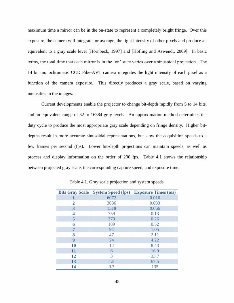
45
maximum time a mirror can be in the on-state to represent a completely bright fringe. Over this
exposure, the camera will integrate, or average, the light intensity of other pixels and produce an
equivalent to a gray scale level [Hornbeck, 1997] and [Hofling and Aswendt, 2009]. In basic
terms, the total time that each mirror is in the ‘on’ state varies over a sinusoidal projection. The
14 bit monochromatic CCD Pike-AVT camera integrates the light intensity of each pixel as a
function of the camera exposure. This directly produces a gray scale, based on varying
intensities in the images.
Current developments enable the projector to change bit-depth rapidly from 5 to 14 bits,
and an equivalent range of 32 to 16384 gray levels. An approximation method determines the
duty cycle to produce the most appropriate gray scale depending on fringe density. Higher bit-
depths result in more accurate sinusoidal representations, but slow the acquisition speeds to a
few frames per second (fps). Lower bit-depth projections can maintain speeds, as well as
process and display information on the order of 200 fps. Table 4.1 shows the relationship
between projected gray scale, the corresponding capture speed, and exposure time.
Table 4.1. Gray scale projection and system speeds.
Bits Gray Scale System Speed (fps) Exposure Times (ms)
1 6072 0.016
2 3036 0.033
3 1518 0.066
4 759 0.13
5 379 0.26
6 189 0.52
7 94 1.05
8 47 2.11
9 24 4.22
10 12 8.43
11 6 16.9
12 3 33.7
13 1.5 67.5
14 0.7 135
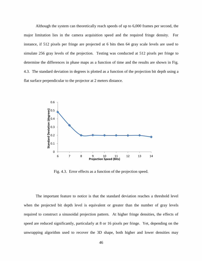
46
Although the system can theoretically reach speeds of up to 6,000 frames per second, the
major limitation lies in the camera acquisition speed and the required fringe density. For
instance, if 512 pixels per fringe are projected at 6 bits then 64 gray scale levels are used to
simulate 256 gray levels of the projection. Testing was conducted at 512 pixels per fringe to
determine the differences in phase maps as a function of time and the results are shown in Fig.
4.3. The standard deviation in degrees is plotted as a function of the projection bit depth using a
flat surface perpendicular to the projector at 2 meters distance.
Fig. 4.3. Error effects as a function of the projection speed.
The important feature to notice is that the standard deviation reaches a threshold level
when the projected bit depth level is equivalent or greater than the number of gray levels
required to construct a sinusoidal projection pattern. At higher fringe densities, the effects of
speed are reduced significantly, particularly at 8 or 16 pixels per fringe. Yet, depending on the
unwrapping algorithm used to recover the 3D shape, both higher and lower densities may
0
0.1
0.2
0.3
0.4
0.5
0.6
6 7 8 9 10 11 12 13 14
Stan
dar
d D
evi
atio
n (
de
gre
es)
Projection Speed (Bits)

47
become an important factor. Additionally, these results are valid amongst a range of distances
from the object to the system, thus representing an overall trend and relationship between the
system speed and potential 3D reconstruction quality.
4.3. Projector-camera software integration
The relationship between the projector and camera are critical for true representations of
the sinusoidal projection. Software developments and improvements were made for integration
of the varying bit depths, speeds, and camera triggering for the fringe projection system
[Harrington et al., 2011]. The CHSLT developed LaserView software was modified
appropriately with a DMD fringe projection module, Fig. 4.4. Options are available to change
resolution of the camera and the center, (x y), position of the AOI of the camera if at values other
than the highest resolution.
Fig. 4.4. LaserView startup selection user selection mode.

48
The type of camera integration can also be chosen. Internal integration is free run of the
camera at video speeds, approximately 60 frames per second. Edge mode-high action is related
to the D4100 Explorer software, which is part of the packaged TI DMD device, and only controls
camera trigger. During this mode, the exposure time can be adjusted directly and maximum
speeds are limited to approximately 25 frames per second by the D4100 Explorer software,
although delays can be added to run at slower speeds. Typically, this mode is used for testing of
different projection patterns developed without direct programming of the DMD chip. The
disadvantage of using the D4100 software is that there is no control of the gray-level. The DMD
device can only be in the on/off state without control of the duty cycle of each mirror. When
experimentation is conducted at this level a common ‘defocusing’ technique is used to remove
sharp discontinuities from the projected image for improved image quality. Level mode-High
action is the programmed, high resolution fringe projection mode used for application testing and
system evaluation. Under this mode, exposure time of the camera is set by the chosen bit depth
from the user. The gray scale level is achieved by now directly varying the duty cycle of the
mirrors and controlling the exposure time of the camera.
In Level mode-High action, the DMD module directly controls the projector via
integration with the programmable FPGA board. When the DMD is enabled via the fringe
projection module, the user can choose from eight preprogrammed fringe densities that are
labeled in terms of pixels per fringe. The highest fringe density reads 4 pixels per fringe and the
density increases by a factor of two up to the broadest fringe density of 512 pixels per fringe,
Fig. 4.5.

49
Fig. 4.5. DMD fringe projection module for LaserView.
Another menu allows the user to choose the projection speed in bits that ranges from 5
bits to 14 bits. When the projection speed exceeds the speed of the camera, integration fails and
the camera begins to capture at non sequential frames, resulting in phase calculation errors.
Depending on the application different number of images can be chosen to calculate the phase
map. LaserView has the option to use 4 phase steps, 8 phase steps, or 16 phase steps. It’s
important to note that for the 8 phase step sequence, the highest fringe density that can be used is
8 pixels per fringe with a 1 pixel phase step. A similar relation exists with the 16 phase step
algorithm; the highest projected density is decreased to 16 pixels per fringe. Thus, there is a
balance between the image quality and the highest spatial resolution in terms of pixels per fringe.
At the same time, using only 4 gray scale levels to model a periodic function could potentially
increase discontinuities and reduce system resolutions. In many cases, the minimum fringe
density is application dependent. For more information on the LaserView software developed,
see [Harrington et al., 2011]
The final feature of the DMD Fringe Projection module is the ability to mathematically
remove the plane of the fringes, in the x and y directions, resulting from the synthetic wavelength

50
produced. This provides users the ability to directly view the fringes from the deformation of the
object. It is important to note that as the density is increased by a factor of two, so too is the
angle of the plane in the x and y directions. Further optimization includes automatic plane
removal based on a fringe counting algorithm to reduce the number of fringes, or groups
bounded by 2π phase jumps in an image.
4.4. First generation prototype
The first generation packaging system, Fig. 4.6, was designed and manufactured with the
intention of having maximum versatility and robustness for a variety of applications. The
enclosure for the projection system was built using stock parts machined on site as well as parts
purchased from outside retailers. The main structural components are two aluminum plates (1)
and four aluminum rails (2) connecting the two plates. Each plate is made of 3/8” 6061
Aluminum while each rail was purchased from 80/20 Incorporated. Holes were drilled into the
aluminum plates to allow for attachment of the four structural rails. Standard fasteners were
used to connect the aluminum rails to the plates.
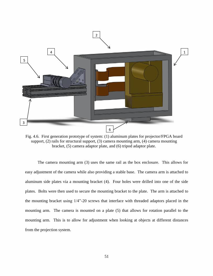
51
The camera mounting arm (3) uses the same rail as the box enclosure. This allows for
easy adjustment of the camera while also providing a stable base. The camera arm is attached to
aluminum side plates via a mounting bracket (4). Four holes were drilled into one of the side
plates. Bolts were then used to secure the mounting bracket to the plate. The arm is attached to
the mounting bracket using 1/4”-20 screws that interface with threaded adaptors placed in the
mounting arm. The camera is mounted on a plate (5) that allows for rotation parallel to the
mounting arm. This is to allow for adjustment when looking at objects at different distances
from the projection system.
1
2
4
6
5
3
Fig. 4.6. First generation prototype of system: (1) aluminum plates for projector/FPGA board
support, (2) rails for structural support, (3) camera mounting arm, (4) camera mounting
bracket, (5) camera adaptor plate, and (6) tripod adaptor plate.
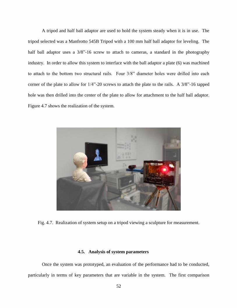
52
A tripod and half ball adaptor are used to hold the system steady when it is in use. The
tripod selected was a Manfrotto 545B Tripod with a 100 mm half ball adaptor for leveling. The
half ball adaptor uses a 3/8”-16 screw to attach to cameras, a standard in the photography
industry. In order to allow this system to interface with the ball adaptor a plate (6) was machined
to attach to the bottom two structural rails. Four 3/8” diameter holes were drilled into each
corner of the plate to allow for 1/4”-20 screws to attach the plate to the rails. A 3/8”-16 tapped
hole was then drilled into the center of the plate to allow for attachment to the half ball adaptor.
Figure 4.7 shows the realization of the system.
Fig. 4.7. Realization of system setup on a tripod viewing a sculpture for measurement.
4.5. Analysis of system parameters
Once the system was prototyped, an evaluation of the performance had to be conducted,
particularly in terms of key parameters that are variable in the system. The first comparison
53
explored the quality of the sinusoidal fringe projection, which essentially determines the quality
of the recovered 3D information. Additionally, the effects of the exposure time and aperture on
the image quality were determined. Finally, a direct comparison was made between 4, 8, and 16
phase step methods in experimental conditions. Each of the evaluated parameters has a direct
effect on the image quality. Understanding these relationship between parameters are key
indicators of appropriate system settings based on the requirements of the application.
4.5.1. Analysis of projected pattern
As explained in the chapter 2, the importance of a sinusoidal projection is critical and
directly related to high frequency noise in unwrapped images. Evaluation of the projection by
images captured from the camera, under laboratory conditions is critical. As verification, a
diffusive, flat surface was setup. For evaluation purposes, a 25 mm telecentric lens with a
limited FOV was used to reduce distortions. The projected pattern, at 128 pixels per fringe, and
the corresponding cross section in Fig. 4.8 shows the ability to successfully project sinusoidal
images from the SLM. A cross-section analysis was conducted on the captured image. The
intensity can be seen as a function of the pixel value along the x-axis.

54
Fig. 4.8. Analysis of projected fringe pattern: (a) capture fringe pattern at 128 pixels per fringe;
and (b) corresponding cross section.
For this particular test, there were sufficient gray scale values to accurately resolve the
sinusoidal pattern. Yet, it’s important to note the direct relation between the number of gray
scales used and the fringe density. At high densities, such as 4 pixels per fringe, only 4 gray
levels are used to reconstruct the sinusoidal pattern.
4.5.2. Effects of exposure time and aperture on image quality
The most important quality of each and every measurement is a large dynamic range of
gray scales that represents the 3D information of the object shape. One of the ways to improve
the dynamic range is by physically increasing the angle of the camera in reference to the object.
Another way is to ensure that each measurement has the maximum contrast without saturation.
By viewing a histogram of the raw data, the parameter of the exposure should be optimized
0 100 200 300 400 500 600
2000
4000
6000
8000
10000
12000
14000
16000
Pixels
Lig
ht
Inte
nsity
Sinusoidal Fringe Projection
(a) (b)
55
based on the largest gray scale range. This ensures the most variation from pixel to pixel and an
improved quality of the 3D information.
In order to directly test the effects of the exposure time, information was gathered at two
different exposures and F/#. The exposure time represents the amount of time photons of light
are reaching the sensor of the camera and the F/# is representing the diameter of the aperture of
the lens. As the F/# increases, the amount of photons hitting the sensor of the camera decreases.
In Table 4.2, the wrapped phases and spatially unwrapped phases are shown. Additionally, the
corresponding histograms with the dynamic range of the gray scale are shown. The images were
captured at 14 bits, corresponding to 16,384 gray scale levels, which is the x-axis of the
displayed histograms.

56
Table 4.2. Comparison of exposure time and F/# on image quality.
An analysis was conducted on each set of unwrapped images to quantify which set had
the better image quality. One indirect method was to look at the cross section of the data across
one line of the sculpture. The high frequency noise in the cross section would be directly visible
in the power spectrum in the frequency domain. As a result, a 1D FFT of each cross section was
taken and compared. Thus, larger signal amplitudes mean nosier images. A direct comparison is
Measurement at F/#: 1.8 and
Exposure Time: 0.995 ms
Measurement at F/#: 2.8 and Exposure
Time: 8.155 ms
Raw
Images
Unwrapped
Phase
Histogram
of Raw
Images

57
0 50 100 150 200 250 300 350-3
-2
-1
0
1
2
3
4
5
6
0 50 100 150 200 250 300 350-3
-2
-1
0
1
2
3
4
5
6
1D FFT y=400
Frequency (Hz)
1D FFT y=400
Frequency (Hz)
shown in Fig. 4.9 in terms of decibels. Again, the logarithmic scale was chosen for viewing
purposes, which is the reason for the portions of power spectrum residing below the zero line.
Fig. 4.9. 1D FFT: (a) poor dynamic range with narrow histogram; and (b) large dynamic range.
Based on the results of the preceding analysis, evaluations on the dynamic range via the
histogram will be conducted prior to making measurements as part of a ‘testing procedure’. The
histogram was added as measurement model in the LaserView software along with cross-section
analysis for convenience. Clearly, improved dynamic range and better contrast reduced high
frequency components in the unwrapped image.
(a) (b)
Am
plit
ud
e (d
b)
Am
plit
ud
e (d
b)

58
4.5.3. Comparison of phase calculation method on image quality
Depending on the requirements of the application, speed has a potential to be an
important factor. Therefore, in all cases, large numbers of phase steps may not be used to
calculate the wrapped phase. In any case, it’s necessary to understand the relationship between
the high frequency noise in images and the number of phase steps used. Theoretically, the more
images used, the greater reduction in the random noise, but experimentation is needed to explore
the magnitude of this effect. Once again, a diffusive, flat surface was setup for measurement.
The camera and aperture setting were kept constant. The wrapped phase map is shown in Fig.
4.10 and was calculated via MatLab.
Fig. 4.10. Wrapped phase maps for 4, 8 and 16 phase steps.
A cross section of the wrapped phase is shown in Fig. 4.11 for all values across the 200th
row. For each case, the arctangent function modulates the data between vales of –π and π.
4 Phase Step
pixels
pix
els
200 400 600 800 1000
200
400
600
800
1000
8 Phase Step
pixels
pix
els
200 400 600 800 1000
200
400
600
800
1000
16 Phase Step
pixels
pix
els
200 400 600 800 1000
200
400
600
800
1000
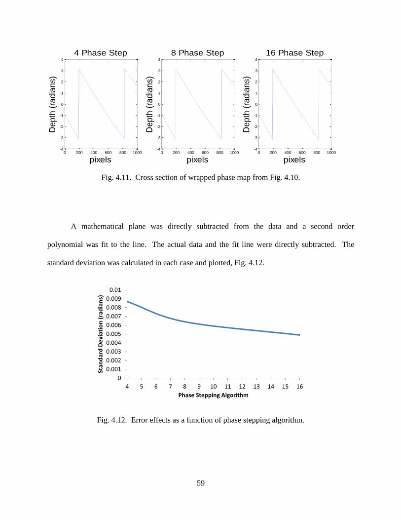
59
Fig. 4.11. Cross section of wrapped phase map from Fig. 4.10.
A mathematical plane was directly subtracted from the data and a second order
polynomial was fit to the line. The actual data and the fit line were directly subtracted. The
standard deviation was calculated in each case and plotted, Fig. 4.12.
Fig. 4.12. Error effects as a function of phase stepping algorithm.
0 200 400 600 800 1000-4
-3
-2
-1
0
1
2
3
4
4 Phase StepD
epth
(ra
dia
ns)
pixels0 200 400 600 800 1000
-4
-3
-2
-1
0
1
2
3
4
8 Phase Step
Depth
(ra
dia
ns)
pixels0 200 400 600 800 1000
-4
-3
-2
-1
0
1
2
3
4
16 Phase Step
pixels
Depth
(ra
dia
ns)
0
0.001
0.002
0.003
0.004
0.005
0.006
0.007
0.008
0.009
0.01
4 5 6 7 8 9 10 11 12 13 14 15 16
Stan
dar
d D
evi
atio
n (
rad
ian
s)
Phase Stepping Algorithm

60
Based on the results, the standard deviation is significantly reduced as a function of the
numbers of images used to calculate the phase. Therefore, just as predicted in the theoretical
case, the electronic noise is reduced as a function of the number of phase steps.
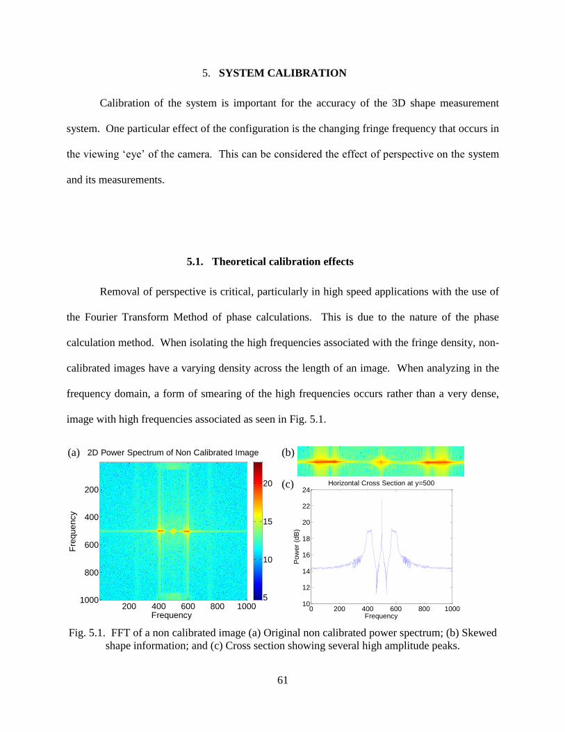
61
0 200 400 600 800 100010
12
14
16
18
20
22
24
Frequency
Pow
er
(dB
)
Horizontal Cross Section at y=500
Frequency
Fre
qu
en
cy
2D Power Spectrum of Non Calibrated Image
200 400 600 800 1000
200
400
600
800
1000 5
10
15
20
5. SYSTEM CALIBRATION
Calibration of the system is important for the accuracy of the 3D shape measurement
system. One particular effect of the configuration is the changing fringe frequency that occurs in
the viewing ‘eye’ of the camera. This can be considered the effect of perspective on the system
and its measurements.
5.1. Theoretical calibration effects
Removal of perspective is critical, particularly in high speed applications with the use of
the Fourier Transform Method of phase calculations. This is due to the nature of the phase
calculation method. When isolating the high frequencies associated with the fringe density, non-
calibrated images have a varying density across the length of an image. When analyzing in the
frequency domain, a form of smearing of the high frequencies occurs rather than a very dense,
image with high frequencies associated as seen in Fig. 5.1.
Fig. 5.1. FFT of a non calibrated image (a) Original non calibrated power spectrum; (b) Skewed
shape information; and (c) Cross section showing several high amplitude peaks.
(a) (b)
(c)
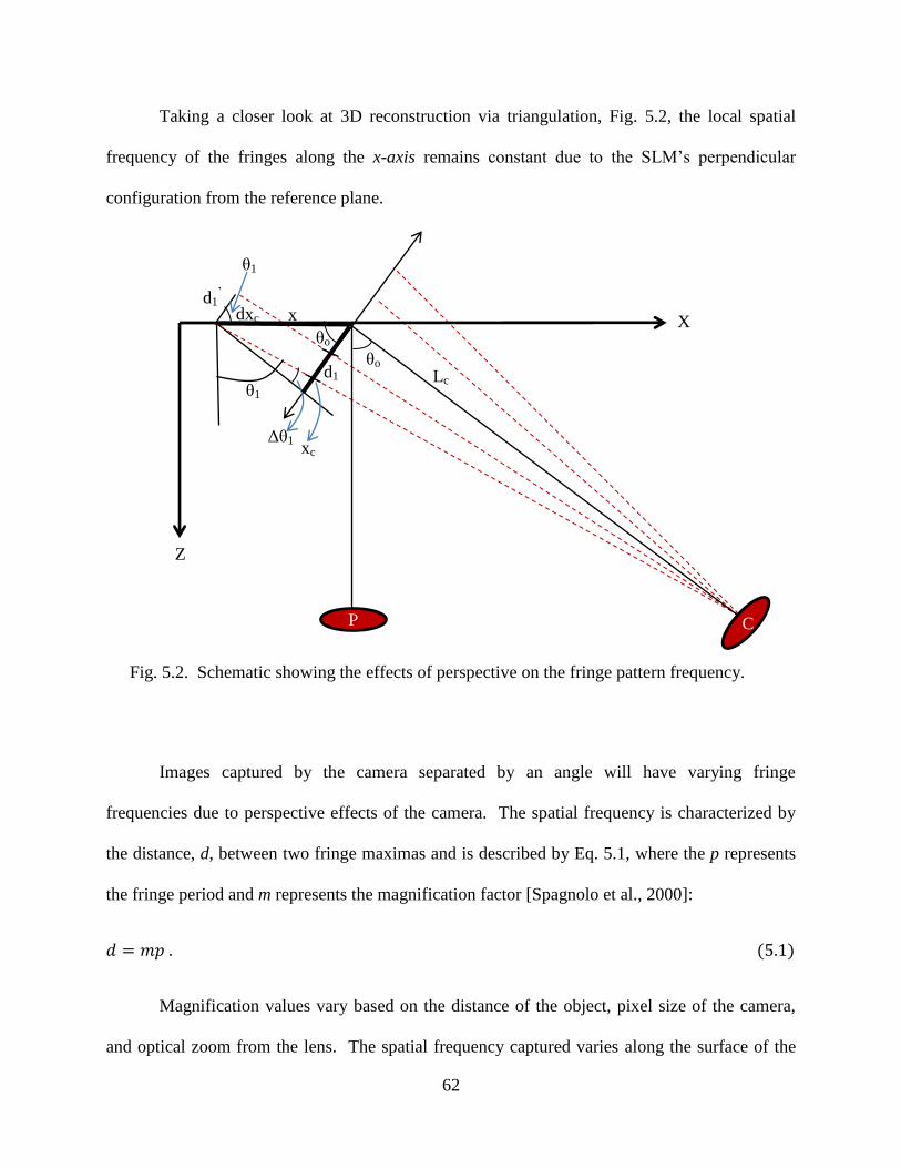
62
Taking a closer look at 3D reconstruction via triangulation, Fig. 5.2, the local spatial
frequency of the fringes along the x-axis remains constant due to the SLM’s perpendicular
configuration from the reference plane.
Images captured by the camera separated by an angle will have varying fringe
frequencies due to perspective effects of the camera. The spatial frequency is characterized by
the distance, d, between two fringe maximas and is described by Eq. 5.1, where the p represents
the fringe period and m represents the magnification factor [Spagnolo et al., 2000]:
Magnification values vary based on the distance of the object, pixel size of the camera,
and optical zoom from the lens. The spatial frequency captured varies along the surface of the
Fig. 5.2. Schematic showing the effects of perspective on the fringe pattern frequency.
θo
θo
d1
d1’
θ1
Lc
dxc
xc
θ1
x
Δθ1
P C
Z
X

63
plane perpendicular to the projector, directly resulting from the angle of the camera. From basic
geometry, the corresponding period viewed by the camera is can be calculated using Eq. 5.2
from Fig. 5.2:
The value of the θ1 needs to be determined. The equations can be simplified by looking
at the right triangle from the center to the calculated fringe period:
Similarly, the following holds true based on similar triangles:
(
)
Substitution of Eqs. 5.4 and 5.5 into Eq. 5.2 result in:
( (
)
[
])
The trigonometric identity described by Eq. 3.13 can be applied to the cosine function in
the denominator of Eq. 5.6 to yield:

64
( (
)
[
] [
])
The camera distance is large as compared with the illumination area of which
means that the cosine value approaches one. Also, the sine function can be approximated to
equal the ratio of over the distance from the camera, Lc. Thus, Eq. 5.7 can be
simplified to:
( (
)
( (
) ))
Knowing that the frequency of the fringes is equal to the inverse of the period, , the
local spatial frequency along the x-axis can be determined. Again, assuming that the value of
and is much larger than the length, Lc, a simplified solution for the local
spatial frequency is shown [Spagnolo et al., 2000]:
(
)
As part of the calibration procedure, it’s important to have an understanding of how an
image is transformed from the real world coordinate system to the coordinate system of the
camera. In order to demonstrate this, a pinhole model was researched.

65
xim
xc
zc
5.2. Pinhole Model
Calibration is a complex task that is critical to accurate 3D reconstruction and has been
studied extensively [Yamauchi et al., 2008]. The developed calibration procedure for the fringe
projection system is based on the pinhole model, Fig. 5.3, that defines both intrinsic and extrinsic
parameters [Yamauchi et al., 2008]. The intrinsic, or internal, parameters include the focal
length, lens distortions, pixel skew factor, and pixel size. The extrinsic parameters include the
position or orientation of the camera. The basic pinhole model defines a geometric relationship
between a 3D point and its 2D corresponding projection based on the center optical axis of the
camera [Morvan et al., 2007].
From basic geometry, the values of x and y on the plane of the image can be scaled
appropriately as follows:
Fig. 5.3 Pinhole model showing the image plane and optical axis

66
where x-value of the image is related to the focal length, the distance of the sensor to the focal
point and its corresponding height dimension. A similar relation can be established for the
scaled y-value. The important factor is the conversion from 3D points in space to the
corresponding 2D points. Figure 5.4 shows a point p on the surface of an object with a
coordinates in the world coordinate system, (xw, yw, zw), and in the camera lens coordinate
system, (xc, yc, zc).
Fig. 5.4 System model schematic
The coordinate of the point of the object as projected on the sensor of the CCD is
represented by point located (u,v). Thus, the relationship between the location of the point on the
object and on the sensor can be modeled mathematically in Eq. 5.12:
[ ]
where s is the scaling factor, I is the homogenous coordinate of the projected imaged on the
sensor such that I=(u,v,1)T in the conversion from Cartesian to homogenous coordinates, and Xw
oc Lens
(u, v)
(uo, vo)
u
v
o
ow
yw
xw
zw
yc
zc
xc
P (xw, yw, zw)
(xc, yc, zc)
Optical Axis
Focal length
CCD sensor
Object

67
is the homogenous coordinate in the world coordinate system such that Xw=(xw, yw, zw, 1)T
[Zhang and Huang, 2006]. Homogenous coordinates are critical in simplification by adding
another term in the coordinate system. Essentially, this allows the use of 3D calibration with the
use of a 2D sensor. Matrix [R, t] compensates for the extrinsic parameters. The intrinsic
matrix A is defined as:
[
]
Point (uo, vo) is the center point of the camera along its optical axis. The variables α and β are
focal lengths along the u and v axis in pixels as described by a linear model. Lastly, γ is the
skew coefficient. Determination of the [R, t] matrix for the extrinsic parameters and the matrix
A for the intrinsic parameters encompasses a complete calibration procedure.
5.3. Calibration Procedure
A calibration procedure was implemented with the use of MatLab. The method was a
combined calibration method that included intrinsic and extrinsic parameters from the camera as
well as distortions from the projector optics. The method was to set up the system parallel to a
diffusive flat surface. The DMD device was programmed to project box patterns with three
varying densities, 8 square pixels per box, 16 square pixels per box, and 32 square pixels per
box. Depending on the FOV of the camera based on the lens and the distance of the object from
the projector, the appropriate density would be used to gather between 15 and 128 control points

68
from the box image. An automated calibration procedure takes an image, Fig. 5.5, and inputs it
into a developed program for outputting the calibration matrix.
Fig. 5.5. Calibration target image captured by the CCD camera.
The algorithm has been optimized for finding the center location of each of the square
based on a type of segmentation procedure. Figure 5.6 shows an example procedure with the
centers of the squares selected.

69
Fig. 5.6. Segmentation Procedure that identifies the center of each box.
A user-defined number of control points are inputted into the program where centers are
chosen randomly throughout the image. A base image is then uploaded, of which size is
automatically cropped to fit the same size based on the numbers of squares. The same sequence
of corresponding square centers is selected in the base image, Fig 5.7.
Fig. 5.7. Control point selection based on idealized target point location.

70
In essence, the program knows where the squares are located in the base image and how
the values are distorted in the captured image. A transformation algorithm is built in that
corrects distortions and outputs the calibration matrix that can be applied to any set of images
taken at this particular configuration. The results of the calibration are shown in Fig. 5.8.
Fig. 5.8. Calibrated image from Fig. 5.6.
In this particular calibration example, the effects of the transformation matrix are difficult
to see visual. Yet, for more practical applications, some information is lost after image
calibration. This phenomenon is due to the correction of the x and y pixels. As the image is
shifted appropriately in space, there are inherently areas of no data so the image is slightly
cropped after calibration.
As validation of the calibration procedure, an algorithm was developed that binarizes the
image based on thresh holding. The top corner of each of each step was selected automatically,
Fig. 5.9. The x pixel position of these points were stored.

71
Fig. 5.9. Calibration verification via detection of corner location on
binary image.
The image before calibration had large perspective effects that distorted the distances
between squares. Yet, in the calibrated images, this effect would be compensated for and the
distances between squares should be the same value. Consequently, the pixel value was plotted
at each location and the results are shown in Fig. 5.10.
0 200 400 600 800-1
-0.5
0
0.5
1
1.5
2Corner Verification
Pixels
Bin
arized I
nte
nsity
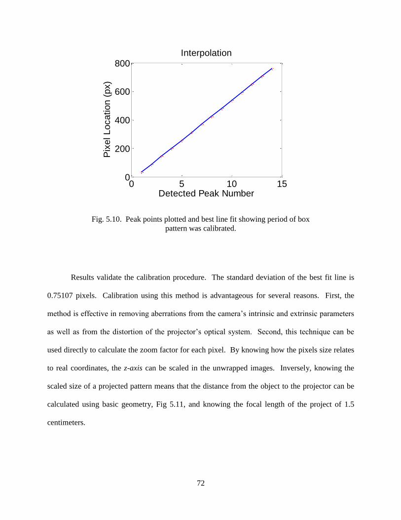
72
Fig. 5.10. Peak points plotted and best line fit showing period of box
pattern was calibrated.
Results validate the calibration procedure. The standard deviation of the best fit line is
0.75107 pixels. Calibration using this method is advantageous for several reasons. First, the
method is effective in removing aberrations from the camera’s intrinsic and extrinsic parameters
as well as from the distortion of the projector’s optical system. Second, this technique can be
used directly to calculate the zoom factor for each pixel. By knowing how the pixels size relates
to real coordinates, the z-axis can be scaled in the unwrapped images. Inversely, knowing the
scaled size of a projected pattern means that the distance from the object to the projector can be
calculated using basic geometry, Fig 5.11, and knowing the focal length of the project of 1.5
centimeters.
0 5 10 150
200
400
600
800Interpolation
Detected Peak Number
Pix
el Location (
px)
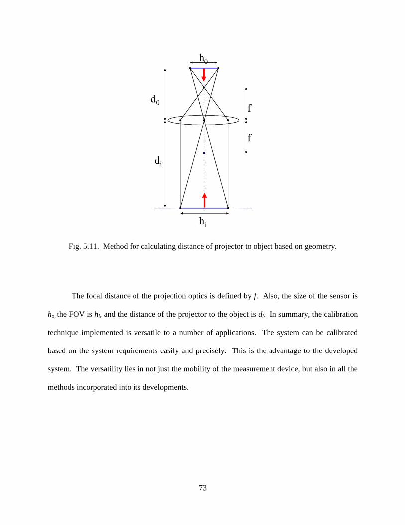
73
Fig. 5.11. Method for calculating distance of projector to object based on geometry.
The focal distance of the projection optics is defined by f. Also, the size of the sensor is
ho, the FOV is hi, and the distance of the projector to the object is di. In summary, the calibration
technique implemented is versatile to a number of applications. The system can be calibrated
based on the system requirements easily and precisely. This is the advantage to the developed
system. The versatility lies in not just the mobility of the measurement device, but also in all the
methods incorporated into its developments.
74
6. DEMONSTRATION OF SYSTEM CAPABILITIES
The capability to measure 3D information is only as useful as the precision and accuracy
of the system. Demonstrating these features validates the applicability prior to making
measurements in field conditions. Additionally, based on the results, the resolution, in (x, y, z),
can be determined.
6.1. Measurement accuracy and resolution
Using the developed system in a single fixed position and the techniques outlined in
chapter 5, the accuracy of the system was evaluated. The relative parameters of the system were
measured mathematically, via calibration and imaging of a measuring device, Fig. 6.1a. The
number of pixels over a 30.5 cm (12.0 inch) length was evaluated to give the size of the scaled
pixel, approximately 0.4031 mm per pixel (0.01587 inches per pixel). Knowing this value, the
size of the square in the calibration matrix was determined. Thus, the distance L of
approximately 114.3 cm (45.0 inches) from the object to the projector was determined by
knowing the corresponding number of pixels per square projected from the system, Fig. 6.1b.
The same is valid for the wavelength in inches at the focus plane, knowing the 32 pixels per
fringe, the wavelength, λ, is 2.52 cm per fringe (0.99 inches per fringe). The fixed distance from
the projector to camera, D, was set at 61.0 cm (24.0 inches).
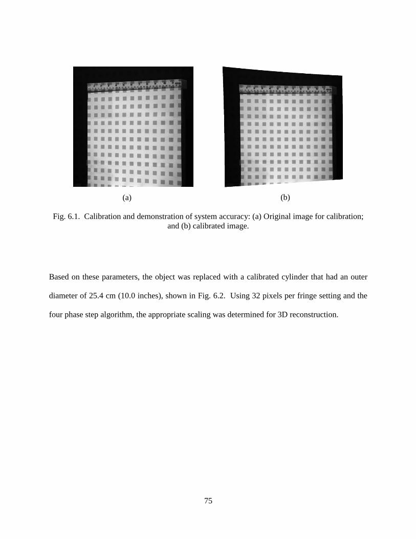
75
Fig. 6.1. Calibration and demonstration of system accuracy: (a) Original image for calibration;
and (b) calibrated image.
Based on these parameters, the object was replaced with a calibrated cylinder that had an outer
diameter of 25.4 cm (10.0 inches), shown in Fig. 6.2. Using 32 pixels per fringe setting and the
four phase step algorithm, the appropriate scaling was determined for 3D reconstruction.
(a) (b)

76
Fig. 6. 2. Calibrated cylinder testing for demonstration of accuracy.
Figure 6.3 shows a 3D representation of the cylinder with appropriately scaled x, y, z
axies, all values are set in centimeters.
Fig. 6.3. Normalized, scaled 3D representation of cylinder.

77
0 5 10 15
-4
-2
0
2
4
6
8
Distance (cm)
Z-D
ep
th (
cm
)
Cross Section at line 250
Extracting a cross-section from this data, the height variation can be viewed, Fig. 6.4,
along position line 250.
Fig. 6.4. Measured cylinder cross section from Fig. 6.3.
The most important evaluation is in the calculation of the cylinder radius measured from the
fringe projection system and comparing this result against the value of the calibrated cylinder. A
method for calculating this radius value was incorporated based on the curvature of the surface,
Eq. 6.1.
| |
| |
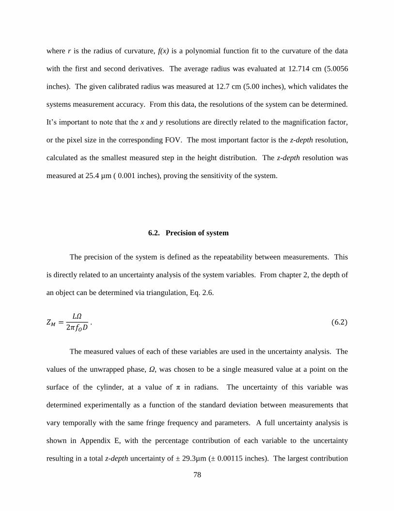
78
where r is the radius of curvature, f(x) is a polynomial function fit to the curvature of the data
with the first and second derivatives. The average radius was evaluated at 12.714 cm (5.0056
inches). The given calibrated radius was measured at 12.7 cm (5.00 inches), which validates the
systems measurement accuracy. From this data, the resolutions of the system can be determined.
It’s important to note that the x and y resolutions are directly related to the magnification factor,
or the pixel size in the corresponding FOV. The most important factor is the z-depth resolution,
calculated as the smallest measured step in the height distribution. The z-depth resolution was
measured at 25.4 µm ( 0.001 inches), proving the sensitivity of the system.
6.2. Precision of system
The precision of the system is defined as the repeatability between measurements. This
is directly related to an uncertainty analysis of the system variables. From chapter 2, the depth of
an object can be determined via triangulation, Eq. 2.6.
The measured values of each of these variables are used in the uncertainty analysis. The
values of the unwrapped phase, Ω, was chosen to be a single measured value at a point on the
surface of the cylinder, at a value of π in radians. The uncertainty of this variable was
determined experimentally as a function of the standard deviation between measurements that
vary temporally with the same fringe frequency and parameters. A full uncertainty analysis is
shown in Appendix E, with the percentage contribution of each variable to the uncertainty
resulting in a total z-depth uncertainty of ± 29.3µm (± 0.00115 inches). The largest contribution
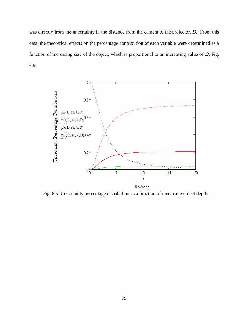
79
was directly from the uncertainty in the distance from the camera to the projector, D. From this
data, the theoretical effects on the percentage contribution of each variable were determined as a
function of increasing size of the object, which is proportional to an increasing value of Ω, Fig.
6.5.
Fig. 6.5 Uncertainty percentage distribution as a function of increasing object depth.

80
From the graph in Fig. 6.5, it’s clear that the as the size of the object increases, the
percentage contribution from the value of the distance, D, becomes the highest source of
uncertainty. The effects propagate significantly over approximately π radians until they level off
at a threshold value. Another interesting effect that can be theoretically evaluated is the effects
of the uncertainty in the z-depth as a function of the size of the object, Fig. 6.6.
As the size of the object increases, the uncertainty in the z-depth also increases. These
effects are only as significant as the required resolution of the application. Yet, the major result
to note is that the uncertainty is proportional to the object size when the wavelength is
normalized based on pixel size. Additionally, an assumption is made that the degradation of
focus from the fringes does not constitute a major source of error, although it could potentially
Fig. 6.6 z-depth uncertainty as a function of increasing object depth.

81
play a large role in the system error. These effects are yet to be determined and could be the
limiting factor for the depth of the object under measurement.

82
7. REPRESENTATIVE APPLICATIONS
As validation of the systems versatility and robustness in a variety of applications and
conditions, several applications are outlined. The first application was in collaboration with
Trilion Optical Test Systems and Northeastern University for the quantification of potholes and
cracks in the road. The key attributes of this test were high speed performance under instable
conditions. The second test was conducted in collaboration with the Worcester Art Museum
(WAM) to digitize an ancient sculpture. The key attribute for this test was accuracy. Both of
these applications have completely different requirements and directly test the versatility of the
system in environments outside the laboratory.
7.1. Road measurements at driving speeds
Potholes, cracks and uneven pavement cost the average driver approximately $400 each
year [Cal Watchdog, 2011]. These conditions can occur as a result of weather, wear, car
accidents, or construction and are a danger to both drivers and pedestrians. Therefore, it is
important to be able to record and evaluate these conditions so that a base for improvement can
be identified.
VOTERS (Versatile Onboard Traffic Embedded Roaming Sensors) is a project designed
to provide an accurate, detailed road assessment and maintenance system. The program is part
of the National Institute of Standards and Technology’s (NIST) Technology Innovation Program
that supports “innovative and high-risk, high-reward research in areas of critical need”
[VOTERS, 2010]. Its overall goals involve a sensing and detecting system that can be adhered
to a vehicle in order to map out large areas. There are three main sensing subsystems to be

83
developed for this project to gather maximum information of road quality. Acoustic systems will
be used to measure particle interaction with tires during normal driving, ground penetrating radar
will be used to subsurface delamination and corrosion, and optical profilometry will be used to
measure surface profiles and detect anomalies. With the development of the 3D shape
measurement system, our system was chosen to be tested for the detection of cracks at driving
speeds. Other portions of the project are in collaboration with Northeastern University, Trilion
Optical Test Systems, The University of Vermont, UMASS Lowell, and Earth Science Systems
(ESS).
The team at Worcester Polytechnic Institute is working on the Surface Optical
Profilometry Roadway Analysis (SOPRA). The aims are to use optical techniques to map out
details such as crack depth. By addressing a compelling societal need, this system has many
applications. Eventually, the surface profiles can be expanded to aid in bridge maintenance.
Global positioning systems can use thresholding algorithms that warn of cracks of particular
dimensions or depth that need maintenance.
The system is incorporated into USPS vans, which means that there is no disruption to
daily traffic. This saves time and money by providing real-time information and eliminating the
need for work zone analysis. This positively impacts the environment by eliminating additional
vehicles and gas consumption to conduct testing. Also, the compact instrument package does
not affect the driver, who does not need to interact with the system while it collects data [NIST,
2009].
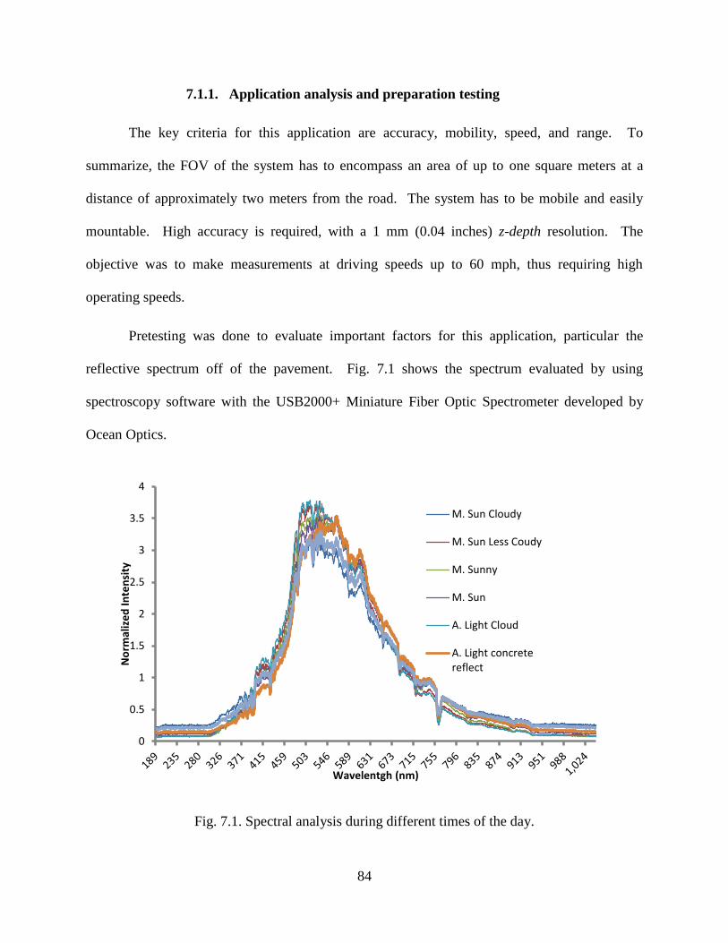
84
7.1.1. Application analysis and preparation testing
The key criteria for this application are accuracy, mobility, speed, and range. To
summarize, the FOV of the system has to encompass an area of up to one square meters at a
distance of approximately two meters from the road. The system has to be mobile and easily
mountable. High accuracy is required, with a 1 mm (0.04 inches) z-depth resolution. The
objective was to make measurements at driving speeds up to 60 mph, thus requiring high
operating speeds.
Pretesting was done to evaluate important factors for this application, particular the
reflective spectrum off of the pavement. Fig. 7.1 shows the spectrum evaluated by using
spectroscopy software with the USB2000+ Miniature Fiber Optic Spectrometer developed by
Ocean Optics.
Fig. 7.1. Spectral analysis during different times of the day.
0
0.5
1
1.5
2
2.5
3
3.5
4
No
rmal
ize
d In
ten
sity
Wavelentgh (nm)
M. Sun Cloudy
M. Sun Less Coudy
M. Sunny
M. Sun
A. Light Cloud
A. Light concretereflect

85
The data shown in Fig. 7.1 is normalized for comparative purposes to see effects during
different times of the day, both morning and afternoon, with and without cloud cover, and
reflectivity off concrete and asphalt. Camera filter’s based on the wavelength of our system,
approximately 620 ± 20 nm, improves contrast and must be used in this application. It’s
important to note that the spectrum intensity is reduced by a factor of approximately 300 under
the reflected concrete and asphalt conditions as compared to ‘A. Light Cloud’ at a wavelength of
620.4 nm.
7.1.2. System setup and integration
A general testing procedure was developed via collaboration with Northeastern
University. A Chevy Express van for testing was provided with an environmentally isolated
camera housing system. The van had already been optimized for road measurements with the
integration of UPS, GPS, and mounting beams on the van roofing. Through collaboration, our
setup was modified for the attachment to the mounting beam off the roof. A preliminary design
of the mounting configuration can be seen in Appendix F, with the incorporation of both the
camera and projector using a 3 beam system. In the final stages of the iterative design process
and via collaboration with Northeastern University, an optimized configuration was chosen by
the adding an adapter plate used to attach the system to the mounting unit. Therefore, the entire
system was directly attached to a single ten foot mounting beam from 80/20 Inc., product 2040,
Fig. 7.2. The camera was attached to another parallel 80/20 Inc. ten foot 2040 beam.
86
Fig. 7. 2. Realization of system mounted onto the van at Northeastern University.
The system was to run with a Pike AVT F-505, 5 megapixel camera to achieve the
desired resolution at the given FOV and distance from the road. The camera pixel size was 3.4 x
3.4 µm2. The maximum frame rate at this resolution is 15 fps, which would gather single images
for FFT analysis. To create a continuous animation of the road, captured frames must be
overlapped by a minimum of 50 percent. Therefore, using this criterion as a baseline and
knowing that each frame covers one full meter minimum, the maximum speed of the van under
current conditions was calculated to be 16.8 mph, which was obtained by:
One of the major concerns for this application is the effects of vibrations on the system.
Future work would focus on improving the stability and reducing vibrations that could affect
(a) (c)
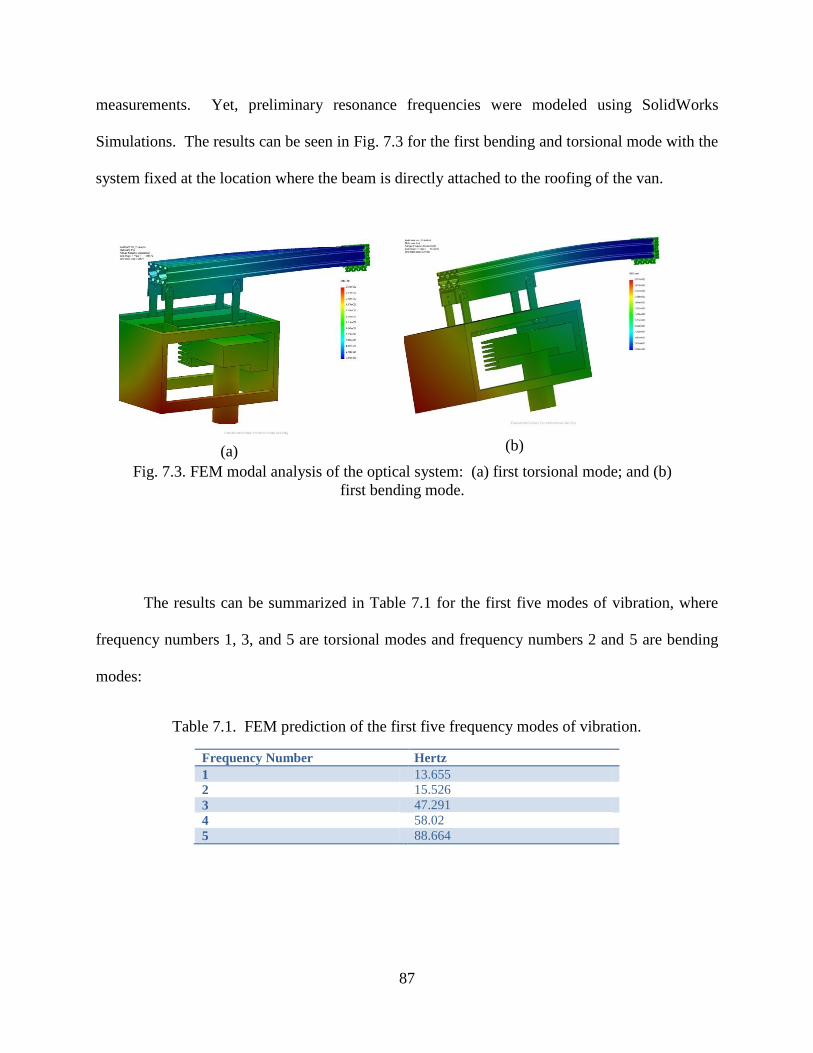
87
measurements. Yet, preliminary resonance frequencies were modeled using SolidWorks
Simulations. The results can be seen in Fig. 7.3 for the first bending and torsional mode with the
system fixed at the location where the beam is directly attached to the roofing of the van.
The results can be summarized in Table 7.1 for the first five modes of vibration, where
frequency numbers 1, 3, and 5 are torsional modes and frequency numbers 2 and 5 are bending
modes:
Table 7.1. FEM prediction of the first five frequency modes of vibration.
Frequency Number Hertz
1 13.655
2 15.526
3 47.291
4 58.02
5 88.664
(b) (a)
Fig. 7.3. FEM modal analysis of the optical system: (a) first torsional mode; and (b)
first bending mode.

88
The results are important because they show another limitation of the current developed
system for use at higher speeds. Cross winds, amongst many other factors, will generate to large
vibration modes that will have to be corrected for in the data analysis. For that reason, lower
speeds from 0-10 mph were used for testing. A more complex mounting system would be used
for the final integration of the system.
Calibration was done by using the same procedure as outline in chapter 4. Yet, in this
case, the system was calibrated once it was attached to the van system. Using a relatively flat
surface and projecting a box pattern, the deformation can be observed and calibration matrix
recovered, Fig. 7.4.
(b) (a)
Fig. 7.4. Calibration procedure: (a) original image; and (b) calibrated image.
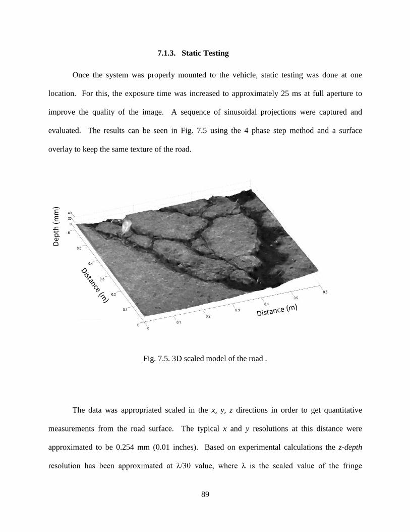
89
7.1.3. Static Testing
Once the system was properly mounted to the vehicle, static testing was done at one
location. For this, the exposure time was increased to approximately 25 ms at full aperture to
improve the quality of the image. A sequence of sinusoidal projections were captured and
evaluated. The results can be seen in Fig. 7.5 using the 4 phase step method and a surface
overlay to keep the same texture of the road.
Fig. 7.5. 3D scaled model of the road .
The data was appropriated scaled in the x, y, z directions in order to get quantitative
measurements from the road surface. The typical x and y resolutions at this distance were
approximated to be 0.254 mm (0.01 inches). Based on experimental calculations the z-depth
resolution has been approximated at λ/30 value, where λ is the scaled value of the fringe
Dep
th (
mm
)

90
Dep
th (
mm
)
Distance (m)
wavelength. Thus, the z-depth resolution was approximated to be 0.737 mm (0.029 inches)
based on a value of λ of 2.2 cm (0.866 inches). A cross section of the data was taken at 0.4
meters vertically and plotted. The results can be seen in Fig. 7.6.
Fig. 7.6. Quantitative cross section of the road measurement data.
7.1.4. Dynamic testing at driving speeds
Preliminary testing was conducted at speeds ranging from 0-10 mph. Images were
captured and analyzed using FFT methods and the results are displayed in Fig. 7.7.
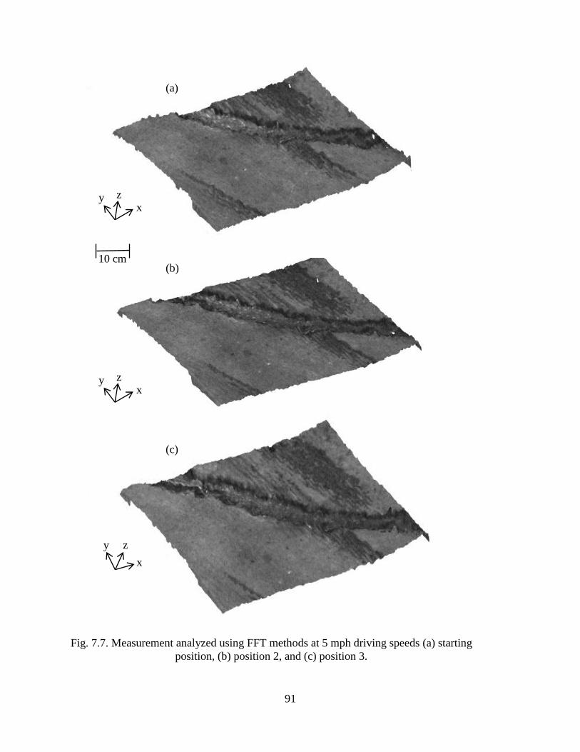
91
Fig. 7.7. Measurement analyzed using FFT methods at 5 mph driving speeds (a) starting
position, (b) position 2, and (c) position 3.
z x
y
z
x
y
z x
y
10 cm
(a)
(b)
(c)
92
The measured speed of the system was completed by knowing the distance travelled
between frames and the exposure time of the camera. Thus, a simple calculation can be
performed to convert to the standard miles per hour. The developed system was successful able
to capture, analyze, and render quality images in instable conditions. This validated the
applicability of the system under dynamic environments. Additional steps will be taken to use
correlation algorithms to stitch images of the road together to create dynamic scenes. Together
with GPS systems, cracks and breaks in the road, such as those identified in Fig. 7.7 would be
flagged for maintenance.
7.2. Sculpture digitization for art conservation
With the overabundance of artwork that has been acquired by museums, the study of art
has become an important phenomenon. Sculptures and other three dimensional art forms portray
important parts of history dating back thousands of years. It is astounding that some have
survived to date. The information and education they can provide to students and art enthusiasts
is endless. Over the recent years, cultural pieces have been threatened by many factors including
population growth, urban development, possible natural disasters, man-made environmental
hazards, and potentially the most dangerous threat - lack of money for preservation [Pieraccini,
2001]. Therefore, preservation of these priceless pieces relates directly to the scientific field via
digitization using non-invasive techniques. Additionally, there is an advantage to having
quantitative 3D representations of models for a number of reasons:
Direct comparison of original models before and after restorations to examine the quality
of the restoration.
93
Visual preview of a restoration before implementation for minimal impact on the
sculpture.
Original ‘vibrant’ color representation can be modified and previewed.
Replication process using a digitized model is safer and quicker than a molding process.
Models can be implemented in a virtual environment for wider use.
As important as it is to study these art forms, conservation is critical for their survival.
However, probes and other similar devices shouldn’t be used because of the artwork’s
sensitivity. In addition, some pieces cannot be moved or placed into a specific area for
measurement. Therefore, there is a great need for a novel non-contact, portable method for art
conservation. This method does not affect the integrity of the sculpture and eliminates the
possibility for damage. It is unique because one can easily transport it to a specific location if the
artwork cannot be moved. For example, this device can be brought on location to archeological
sites. Images can be taken, digitized, sent anywhere within a few hours. This provides fast,
widespread access to information as well as a safe, detailed projection of the artwork. Another
advantage is the affordability of this type of system and simplicity of a developed system for
measurements.
There are several requirements for the system. First, a full field of view must be
available. Next, one must be able to record at large resolutions, which will help to attain details
and greatly aid in art restoration by producing quantitative information as to the size and shape of
the object. For example, using a digitized image, a sculpture can be restored based on the
location of a particular crack. The restoration can be validated simply be digitizing the new
sculpture. Using this technology, one would be able to see what a restoration would look like
prior to applying it. By providing this prediction system, the result is more accurate, realistic

94
restorations. To test the applicability of the system for this type of environment, the system was
tested in laboratory environments and the results can be seen in Fig. 7.8. The results shown are
from a sculpture ‘David’ from a single orientation.
Fig. 7.8. Digitized sculpture in laboratory conditions.
The lab render was successful and has potential for further sculpture digitization. Some
important attributes to consider are the sculptures original colors. The sculpture used in lab
testing was a uniform white, although many ancient sculptures have complex surface colors and
features. By combining this technique with chemical analysis there is a potential to determine
the type and colors of original paint used, thus providing more information on the history of the
piece. One would also be able to use the digitized image to change colors of portions of the
sculpture to more accurately represent the model. This original replica can be used for restoration
or digital record keeping.
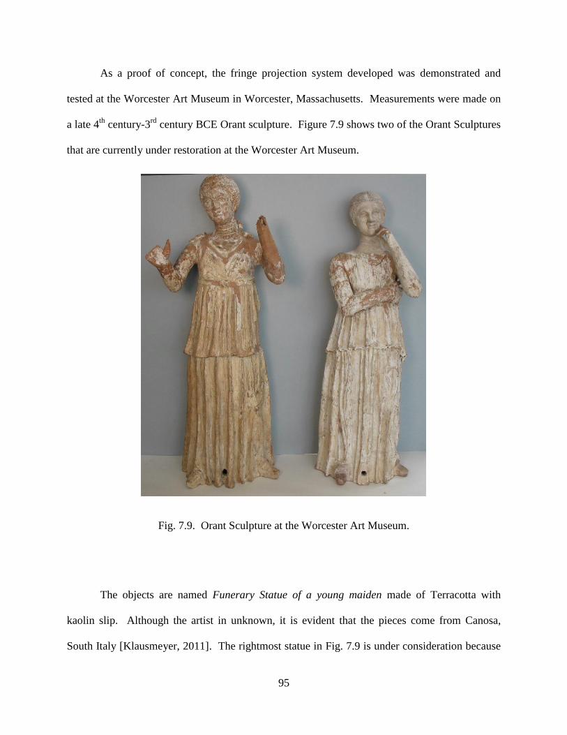
95
As a proof of concept, the fringe projection system developed was demonstrated and
tested at the Worcester Art Museum in Worcester, Massachusetts. Measurements were made on
a late 4th
century-3rd
century BCE Orant sculpture. Figure 7.9 shows two of the Orant Sculptures
that are currently under restoration at the Worcester Art Museum.
Fig. 7.9. Orant Sculpture at the Worcester Art Museum.
The objects are named Funerary Statue of a young maiden made of Terracotta with
kaolin slip. Although the artist in unknown, it is evident that the pieces come from Canosa,
South Italy [Klausmeyer, 2011]. The rightmost statue in Fig. 7.9 is under consideration because
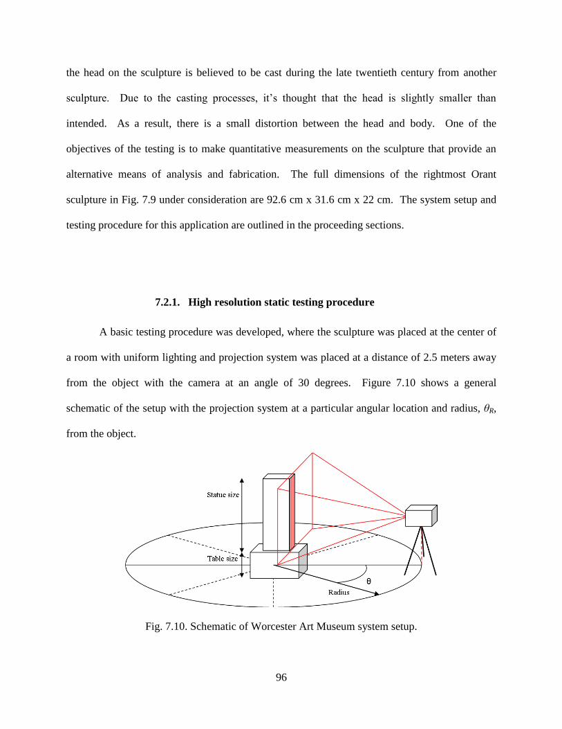
96
the head on the sculpture is believed to be cast during the late twentieth century from another
sculpture. Due to the casting processes, it’s thought that the head is slightly smaller than
intended. As a result, there is a small distortion between the head and body. One of the
objectives of the testing is to make quantitative measurements on the sculpture that provide an
alternative means of analysis and fabrication. The full dimensions of the rightmost Orant
sculpture in Fig. 7.9 under consideration are 92.6 cm x 31.6 cm x 22 cm. The system setup and
testing procedure for this application are outlined in the proceeding sections.
7.2.1. High resolution static testing procedure
A basic testing procedure was developed, where the sculpture was placed at the center of
a room with uniform lighting and projection system was placed at a distance of 2.5 meters away
from the object with the camera at an angle of 30 degrees. Figure 7.10 shows a general
schematic of the setup with the projection system at a particular angular location and radius, θR,
from the object.
Fig. 7.10. Schematic of Worcester Art Museum system setup.
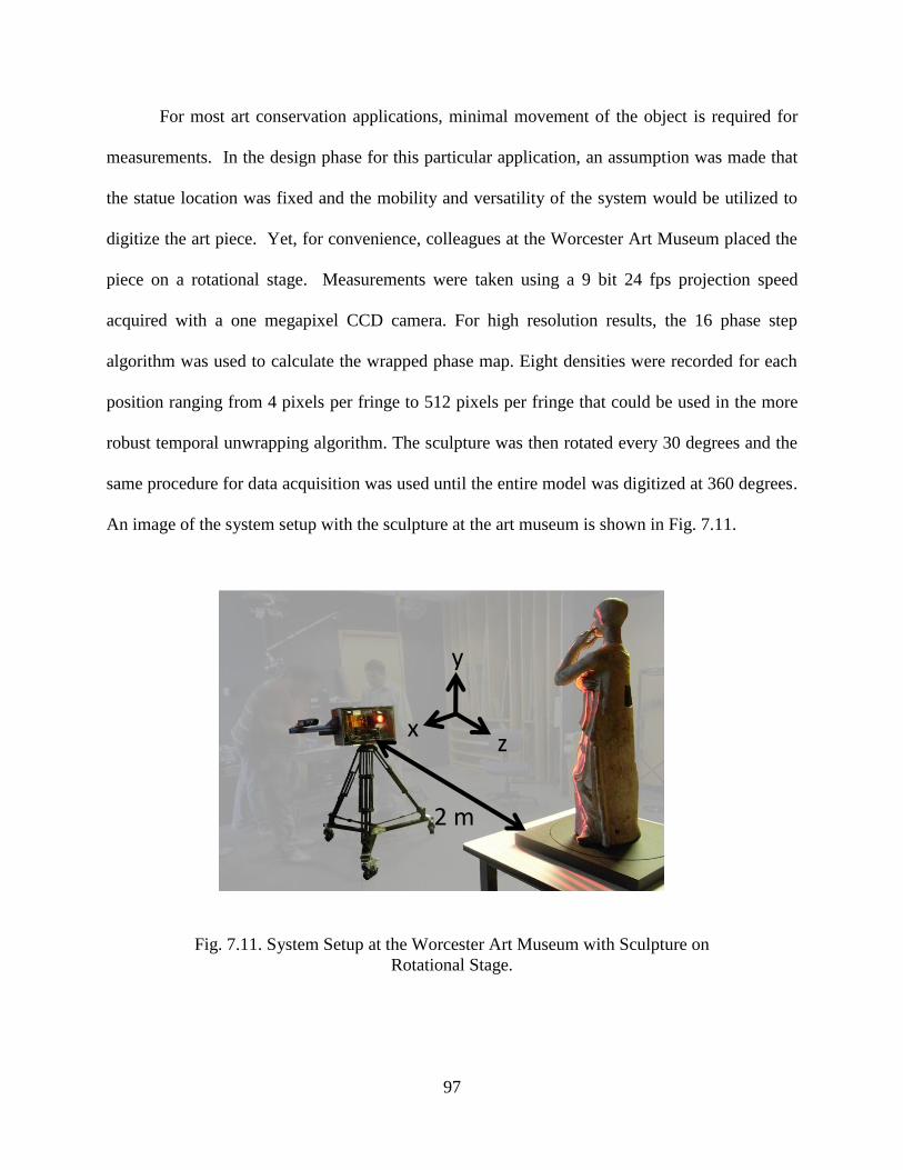
97
2 m
z
y
x
For most art conservation applications, minimal movement of the object is required for
measurements. In the design phase for this particular application, an assumption was made that
the statue location was fixed and the mobility and versatility of the system would be utilized to
digitize the art piece. Yet, for convenience, colleagues at the Worcester Art Museum placed the
piece on a rotational stage. Measurements were taken using a 9 bit 24 fps projection speed
acquired with a one megapixel CCD camera. For high resolution results, the 16 phase step
algorithm was used to calculate the wrapped phase map. Eight densities were recorded for each
position ranging from 4 pixels per fringe to 512 pixels per fringe that could be used in the more
robust temporal unwrapping algorithm. The sculpture was then rotated every 30 degrees and the
same procedure for data acquisition was used until the entire model was digitized at 360 degrees.
An image of the system setup with the sculpture at the art museum is shown in Fig. 7.11.
Fig. 7.11. System Setup at the Worcester Art Museum with Sculpture on
Rotational Stage.
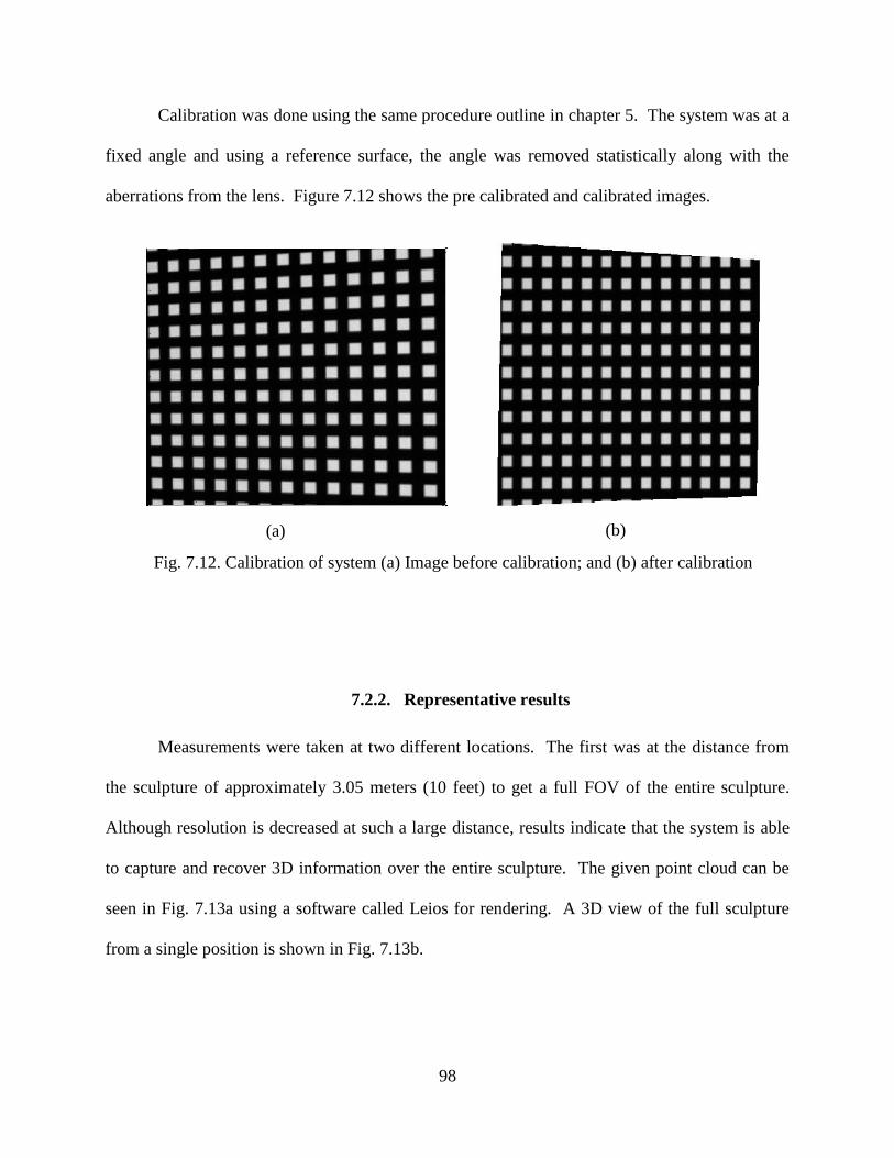
98
Calibration was done using the same procedure outline in chapter 5. The system was at a
fixed angle and using a reference surface, the angle was removed statistically along with the
aberrations from the lens. Figure 7.12 shows the pre calibrated and calibrated images.
7.2.2. Representative results
Measurements were taken at two different locations. The first was at the distance from
the sculpture of approximately 3.05 meters (10 feet) to get a full FOV of the entire sculpture.
Although resolution is decreased at such a large distance, results indicate that the system is able
to capture and recover 3D information over the entire sculpture. The given point cloud can be
seen in Fig. 7.13a using a software called Leios for rendering. A 3D view of the full sculpture
from a single position is shown in Fig. 7.13b.
Calibrated picture
100 200 300 400 500 600
100
200
300
400
500
600
(a) (b)
Fig. 7.12. Calibration of system (a) Image before calibration; and (b) after calibration

99
It’s clear from the analysis that there are effects of shadowing and many views are
needed for full reconstruction of measurements. The second position for measurement
was of approximately 1.2 meters (4 feet) from the sculpture to the system. Similar
system resolutions outlined in chapter 6 are expected at this distance. The reason for
choosing this particular distance was because a focus of the experiment was to resize the
Fig. 7.13. 3D reconstruction of data (a) As viewed in Leios with
mesh; and (b) with color map and shifted orientation.
10 cm
z x
y
(a) (b)
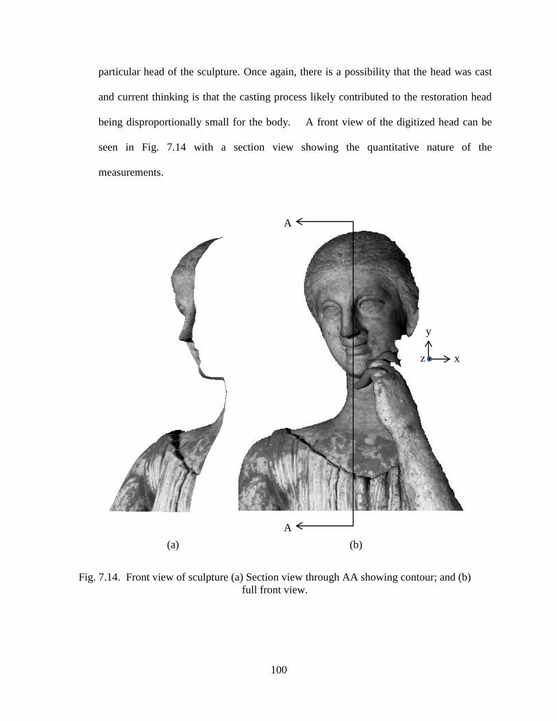
100
particular head of the sculpture. Once again, there is a possibility that the head was cast
and current thinking is that the casting process likely contributed to the restoration head
being disproportionally small for the body. A front view of the digitized head can be
seen in Fig. 7.14 with a section view showing the quantitative nature of the
measurements.
Fig. 7.14. Front view of sculpture (a) Section view through AA showing contour; and (b)
full front view.
z x
y
A
A
(a) (b)

101
One of the objectives for this particular application was to digitize the current head and
increase its size by an appropriate value based on proportions between the head and shoulder size
or the ratio of head to body size. Discussions between curators and conservators on whether to
exhibit the figure with or without the restoration head are ongoing, however 3-D modeling of the
restoration head using fringe projection may offer a third alternative by providing the means by
which to fabricate an accurate reproduction of the restoration head that is proportionally larger
and thus more consistent with the original figure.
The same testing procedure was conducted and the sculpture was again rotated every 30
degrees to gather 360 degrees of information for digitization. Preliminary sculpture results are
shown in Fig. 7.15 from a rotated view of the sculpture.
Fig. 7.15. Front view of sculpture at angled orientation.
z
x
y

102
Data was analyszed from every 30 degree position. To summarize some of the results,
every 90 degree rotation has been analyzed and can be seen in Fig. 7.16. For this analysis, the
original texture of the figure has been mapped over the data. Altough future work is being
conducted on the alterations of the color scheme.
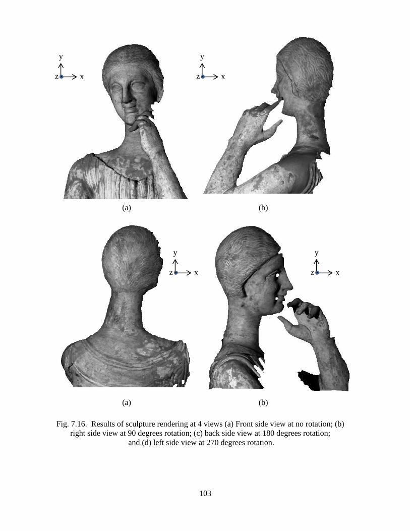
103
Fig. 7.16. Results of sculpture rendering at 4 views (a) Front side view at no rotation; (b)
right side view at 90 degrees rotation; (c) back side view at 180 degrees rotation;
and (d) left side view at 270 degrees rotation.
z x
y
z x
y
z x
y
z x
y
(a) (b)
(a) (b)
104
There are several important points to acknowledge with this particular application. The
task requires images from many angles because the fine details create shadows that make
rendering difficult. Also, to get the full appreciation for fringe projection for art conservation, a
stitching algorithm needs to be developed to render complete models.
7.2.3. Analysis of resolutions and potential improvements
Based on the appropriate distance of the Orant sculpture from the object for the
measurements of the head, the x and y resolution are approximately at 0.381 mm (0.015 inches).
The z-depth resolution was approximated at 68.6 µm (0.0027 inches) based on a fringe
wavelength value of 2.05 mm at its highest density. To improve this resolution there are several
changes to the system that should be made. First, the FOV of the camera and projector should be
matched as precisely as possible. Figure 7.17 shows the extent of the projection area,
approximately 3 meters, to obtain a less than 1 meter FOV from the camera.

105
Fig. 7.17. Projection system FOV at approximately 2 meters form the Orant sculpture.
Additionally, by reducing the size of the pixels on the camera, and increasing the fringe
frequency on the object, there can be even greater improvements on the spatial resolution in x, y,
and z.
In summary, there are many potential applications for this technology and room for
advancements as well. The system has also been tested for forensic applications with footprint
detection and measurements on the surface of United States coins [Hanquier, 2011].
106
8. CONCLUSIONS AND RECOMMENDATIONS
A method for quantitative 3D shape measurements was successfully identified and
developed that provides superior versatility for an endless list of applications. Advanced
algorithms were incorporated into the system for measurement of dynamic scenes and high
resolution static scenes. The versatility is unparalleled in all aspects of the development, from
packaging, to unwrapping and calibration techniques. Evaluations conducted on the final system
validated the theoretical concepts defined by the mathematics.
The system was applied in two contrary applications. The first was for high speed road
measurements where stable conditions were difficult to achieve and high speed acquisition was
necessary. The next was for sculpture digitization at high resolutions where speed was less of a
concern, but accuracy played a critical role. The system successful recovered quantitative 3D
shape information from both of these applications that validate the systems potential.
Future improvements can be made in several aspects of the system. First would be the
packaging. A second generation prototype needs to be developed that incorporates automated
features, particularly changing the angle of the camera, with a direct feedback system that has a
pre calibrated matrix integrated for different camera positions. Secondly, post processing needs
to be streamlined and incorporated into LaserView for real-time 3D viewing. In order to do this
several aspects must be advanced. First, the spatial and temporal unwrapping techniques must be
integrated into the software. Heavy processing power from the software may be required so
algorithm optimization is necessary.
Other visualization improvements need to be made to the system. Optimization of
meshing procedures could reduce high frequencies and more accurately represent the surface
profiles. Additionally, precision stitching of information is necessary in all applications. For

107
instance in the road measurement application, portions of the road need to be linked to create a
‘map’ for better visualization. In art conservation, stitching is needed to view the entire full FOV
of the sculpture. The accuracies of this method are critical in retaining the accuracy of the
system for quantitative measurements. The difficulty lies in the limitation of error propagation
as a function of the number of stitched images.
Overall, the development of the system was successful for quantitative 3D shape
measurements. Interesting developments could be made with the combination of this system
with other optical systems for non-invasive measurements. Some examples include
Shearography [Pryputniewicz, 1992] and Reflective Transformation Imaging (RTI) [Malzbender
et al., 2000].
108
9. REFERENCES
Bothe, T., Osten, W., Gesierich, A., and Juptner, W., “Compact 3D-Camera,” Proc. SPIE,
4778:48-59, 2002.
Burke, J., Bothe, T., Osten, W., and Hess, C., “Reverse Engineering by Fringe Projection,”
Interferometry XI: Applications, Proc. SPIE 4778:312-324, 2002.
Cal Watchdog, On-line: http://www.calwatchdog.com/2011/03/24/wealthy-and-poor-california-
spongers/ , 2011.
Cloud, G., Optical Methods of Engineering Analysis, Cambridge University Press, 1998.
Dodgson, N., “Variation and extrema of human interpupillary distance,” Stereoscopic Displays
and Applications, Proc. SPIE 5291:36-46, 2003.
Dornaika, F. and Hammoudi, K., “Extracting 3D polyhedral Building Models from Aerial
Images using a Featureless and Direct Approach,” Proc. IAPR/MVA 12:378-381, 2009.
Engineers Edge, “Coordinate Measurement Machine CMM About” on-line:
http://www.engineersedge.com/inspection/coordinate_measurement_machine_cmm.htm, 2011.
Furlong, C., Hybrid, experimental and computational, approach for the efficient
study and optimization of mechanical and electro-mechanical components, Ph.D.
dissertation, Worcester Polytechnic Institute, 1999.
Ghiglia, D. C. and Pritt, M. D., Two-Dimensional Phase Unwrapping: Theory, Algorithms, and
Software, John Wiley & Sons, Inc., 1998.
Gonzales, R., Woods, R., Eddins, S., Digital Image Processing using MatLab® Gatesmark
Publishing, 2009.
Gorthi, S. and Rastogi, P., “Fringe projection techniques: whither we are,” Opt. Lasers Engg.,
48:133-140, 2010.
Grimm, T., “Selection Criteria for Common Applications,” T.A. Grimm & Associates, Inc.,
2009.
Hanquier, M., Personal communication with Maxime Hanquier, 2011.
Harrington, E., Furlong, C., Rosowski, J. J., and Cheng, J. T., “Automatic Acquisition and
Processing of Large Sets of Holographic Measurements in Medical Research,” Proc. SEM,
5:219-228, 2011.
Hornbeck, L. J., “Digital Light Processing for High-Brightness, High-Resolution Applications,”
Proc. SPIE, 3013:27-41, 1997.
109
Hofling, R. and Aswendt, P., “Real Time 3D Shape Recording by DLP® Based all-digital
Surface Encoding,” Proc. SPIE, 7210:E-1-E-8, 2009.
Huntley, J. M., and Saldner, H. O., “Shape measurement by temporal phase unwrapping: a
comparison of unwrapping algorithms,” Meas. Sci. Technol. 8:986-992, 1997.
Jia, P., Kofman, J., and English, C., “Comparison of linear and nonlinear calibration methods for
phase-measuring profilometry,” Opt. Engg., 46:043601, 2007.
Kinell, L., Shape Measurements using Temporal Phase Unwrapping, Licentiate Thesis, Lulea
University of Technology, 2000.
Klausmeyer, P., Personal communications with Dr. Klausmeyer from the Worcester Art
Museum, 2011.
Kreis, T., Handbook of Holographic Interferometry, Wiley-VCH Verlag GmbH& Co. KGaA,
Weinheim, 2005.
Malzbender, T., Gelb, D., Wolters, H., Zuckerman, B., “Enhancement of shape
perception by surface reflectance transformation,” Tech. Rep. HPL- 2000-38R1.
Hewlett-Packard Laboratories, Palo Alto, California, 2000.
Morvan, Y., Farin, D., de With, P. H. N., “Acquisition, compression and rendering of multi-view
Video,” NXP Workshop, Eindhoven Technical University, The Netherlands, August 2007.
NIST, Technology Innovation Program: Project Brief, on-line:
http://tipex.nist.gov/tippb/prjbriefs/prjbrief.cfm?ProjectNumber=080046, 2009.
Pieraccini, M., Guidi, G., and Atzeni, C., “3D digitization of cultural heritage,” Journal of
Cultural Heritage 2:63-70, 2001.
Pryputniewicz, R. J., "Electronic shearography and electronic holography working side by side,"
Proc. SPIE, 1821:27-37, 1992.
Salvi, J., Pages, J., Batlle, J., “Pattern Codification strategies in structured light systems,” Pattern
Recognition, 37:827-249, 2004.
Schuon, S., Theobalt, C., Davis, J., and Thrun, S., “High-quality scanning using time-of-flight
depth superresolution,” IEEE Computer Society Conference on Computer Vision and Pattern
Recognition Workshops, 2008.
Sontheimer, A., “Digital Micromirror Device (DMD) Hinge Memory Lifetime,” Texas
Instruments, Inc. DLP Products, 2002.
Spagnolo, G. S., Guattari, G., Sapia, C., Ambrosini, D., Paloetti, D., and Accardo, G.
“Contouring of artwork surface by fringe projection and FFT analysis,” Opt. Lasers Engg.,
33:141-156, 2000.

110
Su, X., Zhang, Q., “Dynamic 3-D shape measurement method: A review,” Opt. Lasers Engg.,
48:191-204, 2010.
Takeda, M., Ina., Hideki, I., and Kobayashi, S., “Fourier Transform method of fringe-pattern
analysis for computer-based topography and interferometry,” J. Opt. Soc. Am, 72:156-160, 1981.
Texas Instruments, “DLP System Optics,” 2010a.
Texas Instruments, “DLP Technology,” on-line: http://www.dlp.com/technology/, 2010b.
Texas Instruments, “DMD 101: Introduction to Digital Micromirror Device (DMD)
Technology,” July 2008.
Van Kessel, P. F., Hornbeck, L., Meier, R., and Douglass, M., R., “A MEMS-based projection
display,” Proc. IEEE, 86:1687-1704, 1998.
VOTERS: Versatile Onboard Traffic Embedded Roaming Sensors, on-line:
http://www.northeastern.edu/voters/documents/VOTERS_one.pdf, 2010.
Whitehouse, D. J., “Review Article: Surface Metrology,” Department of Engineering,
University of Warwick, Coventry, UK, 21 May 1997.
Xiaobo, C., Xi, J., Tao, J., Ye, J., “Research and development of an accurate 3D shape
measurement system based on fringe projection: model analysis and performance evaluation,”
Prec. Engg., 32:215-221, 2008.
Yamauchi, K., Saito, H., and Sato, Y., “Calibration of a structured light system by observing
planar object from unknown viewpoints,” IEEE doi: 10.1109/ICPR.2008.4761303, 2008.
Zervas, M., Furlong, C., Harrington, E., Dobrev, I., “3D shape measurements with high-speed
fringe projection and temporal phase unwrapping,” Proc. SEM, 5:235-241, 2011.
Zhang, S., Huang, P. S., “Novel method for structured light system calibration,” Opt. Engg. 45,
2006.
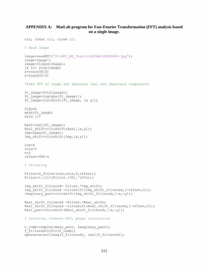
111
APPENDIX A: MatLab program for Fast-Fourier Transformation (FFT) analysis based
on a single image.
clc, clear all, close all
% Read Image
image=readRTI('F:\WPI_MS_Thesis\SOPRA\DSCN2849.jpg'); image=image'; image=flipud(image); [X Y]= size(image) x=round(X/2) y=round(Y/2)
%Take FFT of image and separate real and imaginary components
ft_image=fft2(image); ft_image=log(abs(ft_image)); ft_image=circshift(ft_image, [x y]);
figure mesh(ft_image) Grid off
Real=real(ft_image); Real_shift=circshift(Real,[x,y]); Img=imag(ft_image); Img_shift=circshift(Img,[x,y]);
row=X cols=Y n=3 offset=486-x
% Filtering
Filter=D_Filter(row,cols,0,offset); Filter=1./(1+(Filter./30).^(2*n));
Img_shift_filtered= Filter.*Img_shift; Img_shift_filtered =circshift(Img_shift_filtered,[-offset,0]); Imaginary_part=circshift(Img_shift_filtered,[-x,-y]);
Real_shift_filtered =Filter.*Real_shift; Real_shift_filtered =circshift(Real_shift_filtered,[-offset,0]); Real_part=circshift(Real_shift_filtered,[-x,-y]);
% Convolve, Inverse FFT, phase calculation
C_comb=complex(Real_part, Imaginary_part); Y_Filtered=ifft2(C_comb); wphase=atan2(imag(Y_Filtered), real(Y_Filtered));

112
Appendix B: Least Squares Method for Phase Calculation
∑
∑ ∑ ∑
∑
∑
∑ ∑
∑
∑
∑ ∑
∑
[
]
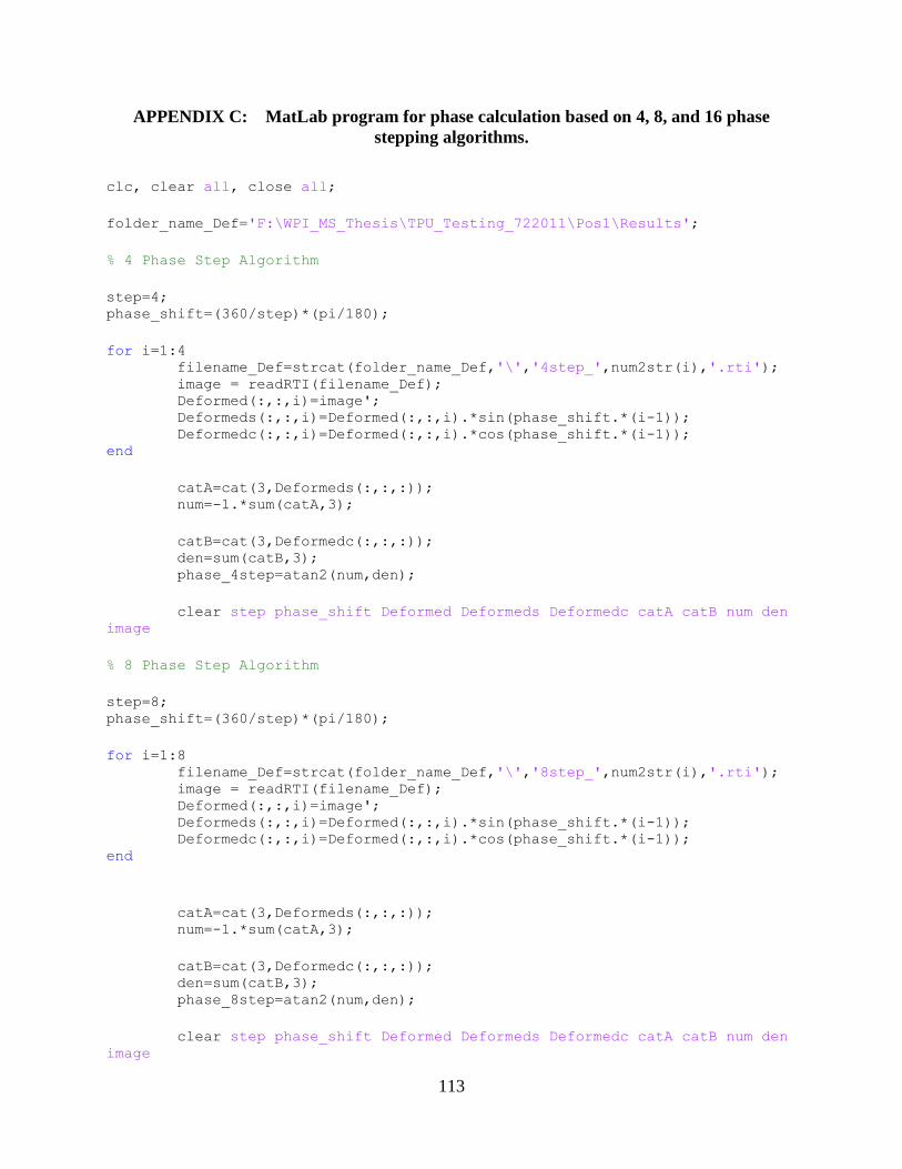
113
APPENDIX C: MatLab program for phase calculation based on 4, 8, and 16 phase
stepping algorithms.
clc, clear all, close all;
folder_name_Def='F:\WPI_MS_Thesis\TPU_Testing_722011\Pos1\Results';
% 4 Phase Step Algorithm
step=4; phase_shift=(360/step)*(pi/180);
for i=1:4 filename_Def=strcat(folder_name_Def,'\','4step_',num2str(i),'.rti'); image = readRTI(filename_Def); Deformed(:,:,i)=image'; Deformeds(:,:,i)=Deformed(:,:,i).*sin(phase_shift.*(i-1)); Deformedc(:,:,i)=Deformed(:,:,i).*cos(phase_shift.*(i-1)); end
catA=cat(3,Deformeds(:,:,:)); num=-1.*sum(catA,3);
catB=cat(3,Deformedc(:,:,:)); den=sum(catB,3); phase_4step=atan2(num,den);
clear step phase_shift Deformed Deformeds Deformedc catA catB num den
image
% 8 Phase Step Algorithm
step=8; phase_shift=(360/step)*(pi/180);
for i=1:8 filename_Def=strcat(folder_name_Def,'\','8step_',num2str(i),'.rti'); image = readRTI(filename_Def); Deformed(:,:,i)=image'; Deformeds(:,:,i)=Deformed(:,:,i).*sin(phase_shift.*(i-1)); Deformedc(:,:,i)=Deformed(:,:,i).*cos(phase_shift.*(i-1)); end
catA=cat(3,Deformeds(:,:,:)); num=-1.*sum(catA,3);
catB=cat(3,Deformedc(:,:,:)); den=sum(catB,3); phase_8step=atan2(num,den);
clear step phase_shift Deformed Deformeds Deformedc catA catB num den
image

114
% 16 Phase Step Algorithm
step=16; phase_shift=(360/step)*(pi/180);
for i=1:16 filename_Def=strcat(folder_name_Def,'\','16step_',num2str(i),'.rti'); image = readRTI(filename_Def); Deformed(:,:,i)=image'; Deformeds(:,:,i)=Deformed(:,:,i).*sin(phase_shift.*(i-1)); Deformedc(:,:,i)=Deformed(:,:,i).*cos(phase_shift.*(i-1)); end
catA=cat(3,Deformeds(:,:,:)); num=-1.*sum(catA,3);
catB=cat(3,Deformedc(:,:,:)); den=sum(catB,3); phase_16step=atan2(num,den);
clear step phase_shift Deformed Deformeds Deformedc catA catB num den
image
figure subplot(1,3,1) imagesc(phase_4step) title('4 Phase Step') xlabel('pixels') ylabel ('pixels')
subplot(1,3,2) imagesc(phase_8step) title('8 Phase Step') xlabel('pixels') ylabel ('pixels')
subplot(1,3,3) imagesc(phase_16step) colormap('gray') title('16 Phase Step') xlabel('pixels') ylabel ('pixels')
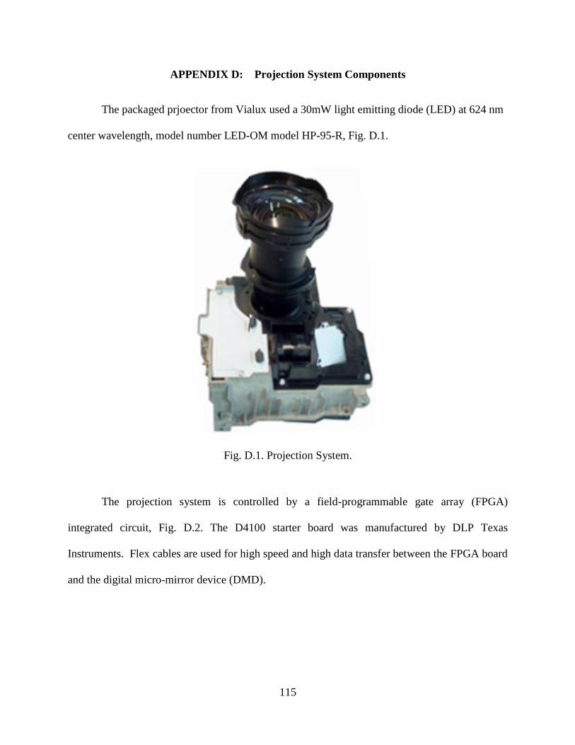
115
APPENDIX D: Projection System Components
The packaged prjoector from Vialux used a 30mW light emitting diode (LED) at 624 nm
center wavelength, model number LED-OM model HP-95-R, Fig. D.1.
Fig. D.1. Projection System.
The projection system is controlled by a field-programmable gate array (FPGA)
integrated circuit, Fig. D.2. The D4100 starter board was manufactured by DLP Texas
Instruments. Flex cables are used for high speed and high data transfer between the FPGA board
and the digital micro-mirror device (DMD).
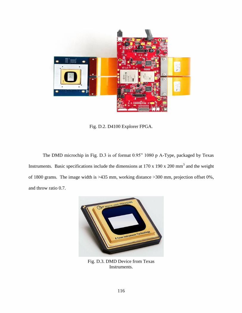
116
Fig. D.2. D4100 Explorer FPGA.
The DMD microchip in Fig. D.3 is of format 0.95” 1080 p A-Type, packaged by Texas
Instruments. Basic specifications include the dimensions at 170 x 190 x 200 mm3 and the weight
of 1800 grams. The image width is >435 mm, working distance >300 mm, projection offset 0%,
and throw ratio 0.7.
Fig. D.3. DMD Device from Texas
Instruments.
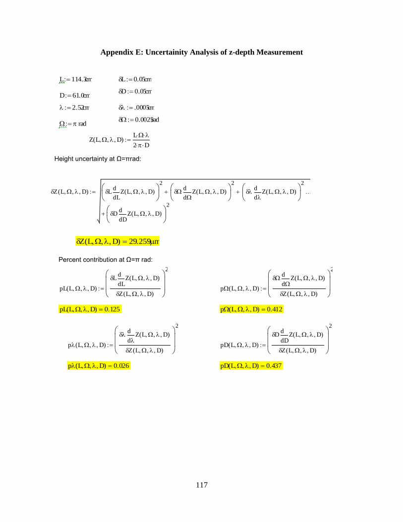
117
Appendix E: Uncertainity Analysis of z-depth Measurement
Height uncertainty at Ω=πrad:
Percent contribution at Ω=π rad:
L 114.3cm L 0.05cm
D 0.05cmD 61.0cm
2.52cm .0005cm
0.0025rad rad
Z L D( )L
2 D
Z L D( ) LL
Z L D( )d
d
2
Z L D( )d
d
2
Z L D( )d
d
2
DD
Z L D( )d
d
2
Z L D( ) 29.259m
pL L D( )
LL
Z L D( )d
d
Z L D( )
2
p L D( )
Z L D( )d
d
Z L D( )
2
pL L D( ) 0.125 p L D( ) 0.412
p L D( )
Z L D( )d
d
Z L D( )
2
pD L D( )
DD
Z L D( )d
d
Z L D( )
2
p L D( ) 0.026 pD L D( ) 0.437
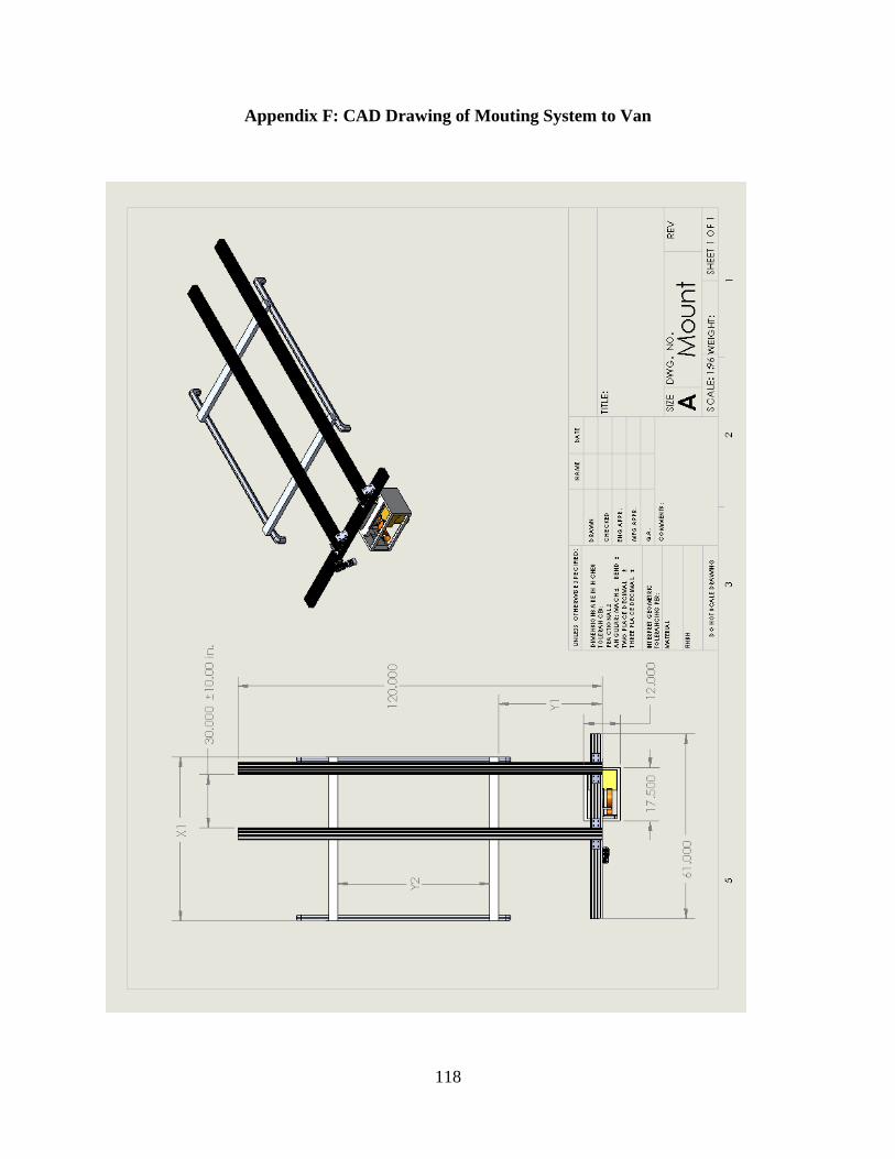
118
Appendix F: CAD Drawing of Mouting System to Van


