International Journal of Applied Mathematics ————————————————————– Volume 30 No. 5 2017, 351-373 ISSN: 1311-1728 (printed version); ISSN: 1314-8060 (on-line version) doi: http://dx.doi.org/10.12732/ijam.v30i5.1 A POSTERIORI ERROR ESTIMATION FOR A DUAL MIXED FINITE ELEMENT METHOD FOR QUASI–NEWTONIAN FLOWS WHOSE VISCOSITY OBEYS A POWER LAW OR CARREAU LAW Mohamed Farhloul 1 § , Abdelmalek Zine 2 1 D´ epartement de Math´ ematiques et de Statistique Universit´ e de Moncton Moncton, N.B., E1A 3E9, CANADA 2 D´ epartement de Math´ ematiques et Informatique Universit´ e de Lyon Institut Camille Jordan, CNRS–UMR5208 Ecole Centrale de Lyon, 36 av. Guy de Collongue 69134 Ecully Cedex, FRANCE Abstract: A dual mixed finite element method, for quasi–Newtonian fluid flow obeying the power law or the Carreau law, is constructed and analyzed in Farhloul–Zine [13]. This mixed formulation possesses good local (i.e., at element level) conservation properties (conservation of the momentum and the mass) as in the finite volume methods. In Farhloul–Zine [12], we developed an a posteriori error analysis for a non–Newtonian fluid flow problems. The analysis is based on the fact that the equation describing the extra–stress tensor in terms of the rate of strain tensor is invertible and may give the rate of strain tensor as a function of the stress tensor. To free ourselves from this constraint of inversion of laws, and as a generalization of the obtained results in [12], we propose in this work an a posteriori error analysis to this mixed formulation. AMS Subject Classification: 65N30, 65N15 Key Words: a posteriori error analysis, dual–mixed formulations, quasi– newtonian, power law, Carreau law Received: July 12, 2017 c 2017 Academic Publications § Correspondence author
Transcript
International Journal of Applied Mathematics————————————————————–Volume 30 No. 5 2017, 351-373ISSN: 1311-1728 (printed version); ISSN: 1314-8060 (on-line version)doi: http://dx.doi.org/10.12732/ijam.v30i5.1
A POSTERIORI ERROR ESTIMATION FOR A DUAL MIXED
FINITE ELEMENT METHOD FOR QUASI–NEWTONIAN
FLOWS WHOSE VISCOSITY OBEYS A POWER LAW OR
CARREAU LAW
Mohamed Farhloul1 §, Abdelmalek Zine2
1Departement de Mathematiques et de StatistiqueUniversite de Moncton
Moncton, N.B., E1A 3E9, CANADA2Departement de Mathematiques et Informatique
Universite de LyonInstitut Camille Jordan, CNRS–UMR5208
Ecole Centrale de Lyon, 36 av. Guy de Collongue69134 Ecully Cedex, FRANCE
Abstract: A dual mixed finite element method, for quasi–Newtonian fluidflow obeying the power law or the Carreau law, is constructed and analyzedin Farhloul–Zine [13]. This mixed formulation possesses good local (i.e., atelement level) conservation properties (conservation of the momentum and themass) as in the finite volume methods. In Farhloul–Zine [12], we developed an a
posteriori error analysis for a non–Newtonian fluid flow problems. The analysisis based on the fact that the equation describing the extra–stress tensor interms of the rate of strain tensor is invertible and may give the rate of straintensor as a function of the stress tensor. To free ourselves from this constraintof inversion of laws, and as a generalization of the obtained results in [12], wepropose in this work an a posteriori error analysis to this mixed formulation.
AMS Subject Classification: 65N30, 65N15Key Words: a posteriori error analysis, dual–mixed formulations, quasi–newtonian, power law, Carreau law
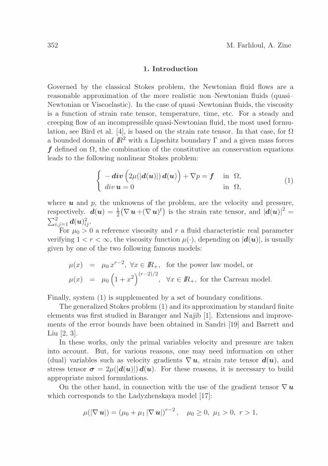
Governed by the classical Stokes problem, the Newtonian fluid flows are areasonable approximation of the more realistic non–Newtonian fluids (quasi–Newtonian or Viscoelastic). In the case of quasi–Newtonian fluids, the viscosityis a function of strain rate tensor, temperature, time, etc. For a steady andcreeping flow of an incompressible quasi-Newtonian fluid, the most used formu-lation, see Bird et al. [4], is based on the strain rate tensor. In that case, for Ωa bounded domain of IR2 with a Lipschitz boundary Γ and a given mass forcesf defined on Ω, the combination of the constitutive an conservation equationsleads to the following nonlinear Stokes problem:
−div(
2µ(|d(u)|)d(u))
+∇p = f in Ω,
div u = 0 in Ω,(1)
where u and p, the unknowns of the problem, are the velocity and pressure,respectively. d(u) = 1
2
(
∇u+(∇u)t)
is the strain rate tensor, and |d(u)|2 =∑2
i,j=1 d(u)2ij .
For µ0 > 0 a reference viscosity and r a fluid characteristic real parameterverifying 1 < r < ∞, the viscosity function µ(·), depending on |d(u)|, is usuallygiven by one of the two following famous models:
µ(x) = µ0 xr−2, ∀x ∈ IR+, for the power law model, or
µ(x) = µ0
(
1 + x2)(r−2)/2
, ∀x ∈ IR+, for the Carreau model.
Finally, system (1) is supplemented by a set of boundary conditions.
The generalized Stokes problem (1) and its approximation by standard finiteelements was first studied in Baranger and Najib [1]. Extensions and improve-ments of the error bounds have been obtained in Sandri [19] and Barrett andLiu [2, 3].
In these works, only the primal variables velocity and pressure are takeninto account. But, for various reasons, one may need information on other(dual) variables such as velocity gradients ∇u, strain rate tensor d(u), andstress tensor σ = 2µ(|d(u)|)d(u). For these reasons, it is necessary to buildappropriate mixed formulations.
On the other hand, in connection with the use of the gradient tensor ∇uwhich corresponds to the Ladyzhenskaya model [17]:
A POSTERIORI ERROR ESTIMATION FOR A DUAL MIXED... 353
a large amount of work is available in the literature. Among these works, theremay be mentioned Manouzi and Farhloul [18], Farhloul and Zine [10], Gaticaet al. [15, 16] and Ervin et al. [9]. The major drawback of formulationsusing the gradient lies in the fact that we can not deal with natural boundaryconditions. To overcome this drawback related to the boundary conditions, wehave introduced and analyzed a dual–mixed finite element method for quasi-Newtonian fluid flow obeying to the power law, in Farhloul and Zine [11, 12]. Apriori error estimates for the finite element approximation were proved in thefirst paper, while a posteriori error estimation was provided in the second work.In both papers, our analysis is based on the fact that the equation describingthe extra–stress tensor in terms of the rate of strain tensor is invertible andgive the rate of strain tensor as a function of the stress tensor. In a recentwork Farhloul–Zine [13], we developed a mixed formulation to overcome thisconstraint of inversibility of the viscosity law. The main advantage of thisformulation is that it makes it possible to consider differently viscosity functionsobeying the power law or Carreau Law.
The aim of this work is to give an a posteriori error estimates for the mixedformulation developed in [13]. In the next Section 2 we recall the mixed for-mulation developed in [13] and then we give the a posteriori error estimatesin Section 3. This will be done by extending our investigations by avoidingthe assumption of expressing the rate of strain tensor as function of the stresstensor. We may be then able to deal with both problems associated with powerlaw and Carreau model.
2. Dual–Mixed Formulation
In order to obtain a dual–mixed formulation of (1), first the problem (1) isformulated as follows:
−div(
σ − p I)
= f in Ω,div u = 0 in Ω,u = 0 on Γ,
(2)
and then, we introduce two new variables
t = d(u), the strain rate tensor, (3)
A(t) = 2µ (|t|) t = σ, the stress tensor. (4)
Let 1 < r < ∞ and r′ being the conjugate number of r, i.e. 1r + 1
r′ = 1.
Suppose f ∈ [Lr′(Ω)]2. Let ω = ω(u) = 12(∇u−(∇u)t) be the vorticity tensor.
354 M. Farhloul, A. Zine
Then, for all (τ , q) ∈ [Lr′(Ω)]2×2 ×Lr′0 (Ω), such that div
(
τ − q I)
∈ [Lr′(Ω)]2,and for all u ∈ [W 1,r(Ω)]2 such that div u = 0, it is easy to see that
one gets(σ,η) = 0, ∀η ∈ [Lr(Ω)]2×2 such that η + ηt = 0.
This corresponds to the symmetry relaxation of the stress tensor σ by a La-grange multiplier.
A POSTERIORI ERROR ESTIMATION FOR A DUAL MIXED... 355
Remark 2. As stated above, the use of the rate of strain tensor en-ables to handle different types of boundary conditions, such as mixed boundaryconditions. More precisely, assuming that we consider the following boundaryconditions:
u = 0 on ΓD and
(2µ(|d(u)|)d(u)− p I) n = 0 on ΓN ,
where Γ = ΓD ∪ ΓN , ΓD 6= ∅ and n is the unit outward normal vector fieldalong the boundary of Ω. Then, the only change to be made is to replace thespace Σ by the following one:
Then, there exists a positive constant β∗ such that
infτ∼
∈Z∗
sups∈T
(s, τ )
‖ s ‖T ‖τ∼
‖Σ≥ β∗.
356 M. Farhloul, A. Zine
Proof. The proof of this result is similar to the one of Lemma 3.6 in [13].
The following result giving the existence, uniqueness and stability is alsoestablished in [13].
Theorem 6. Problem (5) admits a unique solution (t,σ∼
,u∼
) ∈ T ×Σ×M
satisfying the following stability condition,
‖ t ‖T + ‖σ∼
‖Σ + ‖u∼
‖M ≤ C(f),
where C(f) is a positive constant depending on f .
Let us now recall the discrete problem. We assume that the boundary Γof the domain Ω is polygonal. We first give some finite element notations.Let h > 0 and Th a triangulation of Ω into triangles. We assume that thetriangulation Th is regular in the sense of Ciarlet [6]. Let K ∈ Th be an elementof the triangulation, we denote by bK the bubble function defined by
bK(x) = λ1(x)λ2(x)λ3(x), ∀x ∈ K,
λi, i = 1, · · · , 3, being the barycentric co-ordinates with respect to the elementK. For k ∈ IN , let Pk(K) denote the space of polynomials of degree less thanor equal to k on K, and
R(K) =[
P1(K)]2
⊕ IR curl bK ,
where curl bK = (∂bK∂x2, −∂bK
∂x1).
To write the discrete mixed formulation, we introduce the following finitedimensional spaces:
T h =
sh ∈ T ; sh|K ∈ R(K), ∀K ∈ Th
,
Σh =
τh∼
= (τ h, qh) ∈ Σ; τ h|K ∈ [R(K)]2,
qh|K ∈ P1(K), ∀K ∈ Th
,
Mh =
vh∼
= (vh,ηh) ∈M ; vh|K ∈[
P0(K)]2,ηh = θh χ,
θh|K ∈ P1(K),∀K ∈ Th
,
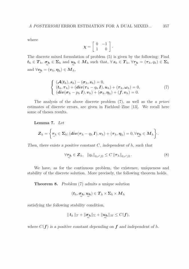
A POSTERIORI ERROR ESTIMATION FOR A DUAL MIXED... 357
where
χ =
[
0 −11 0
]
.
The discrete mixed formulation of problem (5) is given by the following: Findth ∈ T h, σh
As it was mentioned above, the upper bounds of the errors depend on theparameter r > 1. On the other hand, to distinguish the two models, we set:δ = 0 for power law and δ = 1 for Carreau law.
We first consider the case where the parameter r verify 1 < r < 2.
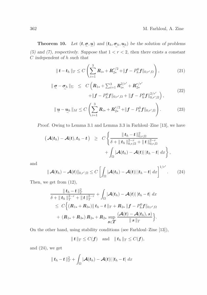
362 M. Farhloul, A. Zine
Theorem 10. Let (t,σ∼
,u∼
) and (th,σh∼
,uh∼
) be the solution of problems
(5) and (7), respectively. Suppose that 1 < r < 2, then there exists a constantC independent of h such that
‖ t− th ‖T ≤ C
(
3∑
i=1
Ri∗+Rr/22∗ +‖f − P 0
hf‖0,r′,Ω
)
, (21)
‖σ∼−σh
∼
‖Σ ≤ C(
R1∗ +∑3
i=1R2/r′
i∗ +Rr/r′
2∗
+‖f − P 0hf‖0,r′,Ω + ‖f − P 0
hf‖2/r′
0,r′,Ω
)
,(22)
‖u∼
−uh∼
‖M ≤ C
(
3∑
i=1
Ri∗+Rr/22∗ +‖f − P 0
hf‖0,r′,Ω
)
. (23)
Proof. Owing to Lemma 3.1 and Lemma 3.3 in Farhloul–Zine [13], we have
(
A(th)−A(t), th− t)
≥ C
‖ th− t ‖20,r,Ω
δ + ‖ th ‖2−r0,r,Ω + ‖ t ‖2−r
0,r,Ω
+
∫
Ω|A(th)−A(t)| |th− t| dx
,
and
‖A(th)−A(t)‖0,r′,Ω ≤ C
[∫
Ω|A(th)−A(t)| |th− t| dx
]1/r′
. (24)
Then, we get from (12),
‖ th− t ‖2T
δ + ‖ th ‖2−rT + ‖ t ‖2−r
T
+
∫
Ω|A(th)−A(t)| |th− t| dx
≤ C
(R1∗ +R3∗)‖ th− t ‖T +R2∗ ‖f − P 0hf‖0,r′,Ω
+ (R1∗ +R3∗)R2∗ +R2∗ sups∈T
(A(t)−A(th), s)
‖ s ‖T
.
On the other hand, using stability conditions (see Farhloul–Zine [13]),
‖ t ‖T ≤ C(f) and ‖ th ‖T ≤ C(f),
and (24), we get
‖ th− t ‖2T +
∫
Ω|A(th)−A(t)| |th− t| dx
A POSTERIORI ERROR ESTIMATION FOR A DUAL MIXED... 363
≤ C
(R1∗ +R3∗)‖ t− th ‖T +R2∗ ‖f − P 0hf‖0,r′,Ω
+R2∗(R1∗ +R3∗) +R2∗
[
∫
Ω|A(th)−A(t)| |th− t| dx
]1/r′
.
Now, using the Young inequality, we obtain, ∀ ε > 0 and ∀ ε > 0,
‖ th− t ‖2T +
∫
Ω|A(th)−A(t)| |th− t| dx
≤ C
ε−1(R1∗ +R3∗)2 + ε‖ t− th ‖
2T
+R2∗ ‖f − P 0hf‖0,r′,Ω +R2∗(R1∗ +R3∗)
+(ε)−r Rr2∗ +(ε)r
′
∫
Ω|A(t)−A(th)| |t− th| dx
.
Thus, for an adequate choice of ε and ε, we get
‖ th− t ‖2T +
∫
Ω|A(th)−A(t)| |th− t| dx ≤ C
(R1∗ +R3∗)2
+R2∗ ‖f − P 0hf‖0,r′,Ω +R2∗(R1∗ +R3∗) +Rr
2∗
.
This implies, in particular, the expected result in equation (21), namely:
‖ t− th ‖T ≤ C(
3∑
i=1
Ri∗ +Rr/22∗ +‖f − P 0
hf‖0,r′,Ω)
,
and∫
Ω |A(th)−A(t)| |t− th| dx
≤ C(
∑3i=1R
2i∗ +Rr
2∗ +‖f − P 0hf‖
20,r′,Ω
)
.(25)
Finally, to obtain the expected estimate (22), it suffices to use the inequalities(20), (24) and (25). And the estimate (23) is a direct consequence of (17) and(21).
After the study of the case 1 < r < 2, we will now consider the case r ≥ 2.
Theorem 11. Let (t,σ∼,u∼) and (th,σh
∼
,uh∼
) be the solution of problems
(5) and (7), respectively. Suppose that r ≥ 2, then there exists a constant C
independent of h such that
‖ t− th ‖T ≤ C(
∑3i=1R
r′/ri∗ +R2∗ +R
2/r2∗
+‖f − P 0hf‖0,r′,Ω
)
,(26)
364 M. Farhloul, A. Zine
‖σ∼
−σh∼
‖Σ ≤ C(
Rr′/21∗ +R
r′/23∗ +
∑3i=1 Ri∗
+‖f − P 0hf‖0,r′,Ω
)
,(27)
‖u∼
−uh∼
‖M ≤ C(
∑3i=1 R
r′/ri∗ +R2∗ +R
2/r2∗
+‖f − P 0hf‖0,r′,Ω
)
.(28)
Proof. Using Lemma 3.2 in Farhloul–Zine [13], we get
(
A(th)−A(t), th− t)
≥ C(
‖ th− t ‖r0,r,Ω
+
∫
Ω
(
δ + |th|r−2 + |t|r−2
)
|th− t|2 dx
)
and
‖A(th)−A(t)‖0,r′,Ω (29)
≤ C
[∫
Ω
(
δ + |th|r−2 + |t|r−2
)
|th− t|2 dx
]1/2
×[
δ + ‖th‖(r−2)/20,r,Ω + ‖t‖
(r−2)/20,r,Ω
]
.
To simplify the notations, we set
Λ = ‖ t− th ‖rT +
∫
Ω
(
δ + |th|r−2 + |t|r−2
)
|t− th|2 dx.
Then, from (12), we have
Λ ≤ C
(R1∗ +R3∗)(‖ th− t ‖T +R2∗) +R2∗ ‖f − P 0hf‖0,r′,Ω
+R2∗ ‖A(th)−A(t)‖0,r′,Ω
.
And then, from (29), we get
Λ ≤ C
(R1∗ +R3∗)(‖ th− t ‖T +R2∗) +R2∗ ‖f − P 0hf‖0,r′,Ω
+R2∗
[∫
Ω
(
δ + |th|r−2 + |t|r−2
)
|th− t|2 dx
]1/2
×(
δ + ‖th‖(r−2)/2T + ‖t‖
(r−2)/2T
)
.
A POSTERIORI ERROR ESTIMATION FOR A DUAL MIXED... 365
And again, using Young’s inequality with two parameters ε and ε, we get
Λ ≤ C
εr‖ th− t ‖rT + ε−r′(R1∗+R3∗)
r′ +R2∗ ‖f − P 0hf‖0,r′,Ω
+ (R1∗ +R3∗)R2∗ +ε
∫
Ω
(
δ + |th|r−2 + |t|r−2
)
|th− t|2 dx
+ (ε)−1 R22∗
(
δ + ‖th‖(r−2)/2T + ‖t‖
(r−2)/2T
)2
.
Thus, using the stability conditions ‖t‖T ≤ C(f) and ‖th‖T ≤ C(f), we obtain
Λ ≤ C
(R1∗ +R3∗)r′ +R2∗ ‖f − P 0
hf‖0,r′,Ω
+(R1∗ +R3∗)R2∗ +R22∗
.(30)
This last inequality leads in particular to
‖ t− th ‖rT ≤ C
(R1∗ +R3∗)r′ +Rr′
2∗ +‖f − P 0hf‖
r0,r′,Ω +Rr
2∗ +R22∗
.
And then,
‖ t− th ‖T ≤ C
3∑
i=1
Rr′/ri∗ +R2∗ +R
2/r2∗ +‖f − P 0
hf‖0,r′,Ω
,
which is precisely the expected estimate (26).
On the other hand, from (30), we deduce the following estimate
∫
Ω
(
δ + |th|r−2 + |t|r−2
)
|t− th|2 dx ≤ C
(R1∗ +R3∗)r′
+(R1∗ +R3∗)2 +R2
2∗ +‖f − P 0hf‖
20,r′,Ω
,
and then, using (20), (29) and the fact that ‖ t ‖T and ‖ th ‖T are bounded, weget
‖σ∼−σh
∼
‖Σ ≤ C
3∑
i=1
Ri∗+Rr′/21∗ +R
r′/23∗ +‖f − P 0
hf‖0,r′,Ω
,
which is the expected estimate (27).
Finally, the estimation (28) is a consequence of the estimates (17) and(26).
366 M. Farhloul, A. Zine
Finally, the previous results show that to have the a posteriori error esti-mates of our problem, it suffices to estimate Ri∗, i = 1, 2, 3. To this end, wefirst precise some notations: for a tensor field τ ∈ IR2×2 and for a vector fieldv = (v1, v2) ∈ IR2,
• tr(τ ) = τ11 + τ22, as(τ ) = τ21 − τ12,
• rot(τ ) =(
∂τ12∂x1
− ∂τ11∂x2
, ∂τ22∂x1− ∂τ21
∂x2
)
,
• Curl(v) =
(
∂v1∂x2
− ∂v1∂x1
∂v2∂x2
− ∂v2∂x1
)
,
• and[[
g]]
Estands for the jump of function g across an edge E.
We also recall the following Helmholtz decomposition of a tensor field in Σ.
Proposition 12. Let τ∼
∈ Σ. Then there exist z ∈[
W 2,r′(Ω)]2
and
ψ ∈[
W 1,r′(Ω)]2
such that
τ − q I = ∇z + Curlψ, (31)
with the estimate‖z‖2,r′,Ω + ‖ψ‖1,r′,Ω ≤ C ‖ τ
∼
‖Σ. (32)
Proof. To prove this result it is sufficient to apply Theorem 1.1 of Creuseet al. [8] to each row of the tensor τ −q I, i.e. the two vector fields (τ11−q, τ12)and (τ21, τ22 − q).
A POSTERIORI ERROR ESTIMATION FOR A DUAL MIXED... 367
• Icl(ψ) is the Clement interpolant of ψ (see Clement [7]),
• Eh denotes the set of all edges of the triangulation Th,
•[[
(th+ωh)t]]
Edenotes the tangential jump of th+ωh across the edge E,
• Πh(∇z) is the Brezzi-Douglas-Marini interpolant of the lowest degree of∇z (see Brezzi et al. [5]).
Proof. By (10), we get for every τ∼
∈ Σ,
< R2, τ∼>= (th+ωh, τ ) + (div(τ − q I),uh).
Then, using the Helmholtz decomposition (31), we get
< R2, τ∼
> = (th+ωh,∇z) + (th+ωh, q I)
+ (th+ωh, Curlψ) + (div(∇z),uh).(34)
On the other hand, using the properties of Πh(∇z), the Brezzi–Douglas–Mariniinterpolant, we get
(div(Πh(∇z)),vh) = (div(∇z),vh), ∀vh ∈[
∏
K∈Th
P0(K)]2.
Thus, using this last relation and the fact that tr(ωh) = 0, the equation (34)may be rewritten as follows:
< R2, τ∼> = (th+ωh,∇z) + (tr(th), q)
+ (th+ωh, Curlψ) + (div(Πh(∇z)),uh).(35)
Taking successively
τh∼
= (Πh(∇z), 0) ∈ Σh and τh∼
= (Curl(Icl(ψ)), 0) ∈ Σh
in the second equation of the discrete problem (7), we obtain
(th+ωh,Πh(∇z)) + (div(Πh(∇z)),uh) = 0
and
(th+ωh, Curl(Icl(ψ))) = 0.
368 M. Farhloul, A. Zine
Injecting these two last relations in the right-hand side of (35), we get
< R2, τ∼
> = (th+ωh,∇z −Πh(∇z)) + (tr(th), q)
+ (th+ωh, Curl(ψ − Icl(ψ))).
Thus, using Green’s formula, we obtain
< R2, τ∼
>=(th+ωh,∇z −Πh(∇z)) + (tr(th), q)
+∑
K∈Th
[(rot(th+ωh),ψ − Icl(ψ))]
−∑
K∈Th
[⟨
(th+ωh)t,ψ − Icl(ψ)⟩
∂K
]
=∑
K∈Th
[
(th+ωh,∇z −Πh(∇z)) + (tr(th), q)]
+∑
K∈Th
[
(rot(th+ωh),ψ − Icl(ψ))]
−∑
E∈Eh
<[[
(th+ωh)t]]
E,ψ − Icl(ψ) >E .
Remark 14. The summation∑
E∈Eh
<[[
(th+ωh)t]]
E,ψ − Icl(ψ) >E
appearing in the right-hand side of formula (33) contains the terms
<[[
(th+ωh)t]]
E,ψ − Icl(ψ) >E,
where E is an edge of the triangulation Th contained in the boundary of Ω; inthis case it must be understood that (th+ωh)t is 0 outside of Ω.
We are now able to give upper bounds of R1∗,R2∗ and R3∗. These upperbounds will be functions of the error indicators η1, η2 and η3. More precisely,we have the following results.
Theorem 15. There exists a constant C independent of h such that
R1∗ ≤(
∑
K∈Th
η1(K)r′
)1/r′
, (36)
A POSTERIORI ERROR ESTIMATION FOR A DUAL MIXED... 369
R2∗ ≤ C(
∑
K∈Th
η2(K)r)1/r
, (37)
R3∗ ≤ C(
∑
K∈Th
η3(K)r′
)1/r′
, (38)
where η1(K), η2(K) and η3(K) are the local estimators given by
η1(K)r′
= ‖A(th)− σh‖r′
0,r′,K ,
η2(K)r = hrK[
‖ th+ωh‖r0,r,K + ‖ rot(th+ωh)‖
r0,r,K
]
+ ‖tr(th)‖r0,r,K +
∑
E∈∂K
hE‖[[
th+ωh)t]]
E‖r0,r,E,
η3(K)r′
= ‖f − P 0hf‖
r′
0,r′,K + ‖as(σh)‖r′
0,r′,K.
Proof. It follows from (9) that for every s ∈ T ,
|< R1, s >| ≤(
∑
K∈Th
‖A(th)− σh‖r′
0,r′,K
)1/r′
‖ s ‖0,r,Ω
and then,
sups∈T
|< R1, s >|
‖ s ‖T≤(
∑
K∈Th
‖A(th)− σh‖r′
0,r′,K
)1/r′
.
Which is precisely the estimate (36). To show the estimate (37), we will use(33) obtained in Lemma 13. This inequality leads, for every τ
∼
∈ Σ, to
| < R2, τ∼> | ≤
∑
K∈Th‖ th+ωh‖0,r,K‖∇z −Πh(∇z)‖0,r′,K
+∑
K∈Th‖tr(th)‖0,r,K‖q‖0,r′,K
+∑
K∈Th‖ rot(th+ωh)‖0,r,K‖ψ − Icl(ψ)‖0,r′,K
+∑
E∈Eh
∥
∥
[[
(th+ωh)t]]
E
∥
∥
0,r,E‖ψ − Icl(ψ)‖0,r′,E.
(39)
Now, by Lemma 3.1 in Verfurth [20], we have
‖ψ − Icl(ψ)‖0,r′,K ≤ ChK |ψ|1,r′,ωK
and
‖ψ − Icl(ψ)‖0,r′,E ≤ Ch1/rE |ψ|1,r′,ωE
,
370 M. Farhloul, A. Zine
where ωK denotes the union of K with all the triangles from the triangulationTh adjacent to the triangle K, ωE denotes the union of at most two trianglesof Th admitting E as a common edge and | · |1,r′,ω, the semi-norm of W 1,r′(ω).
Thus, using these two last estimates and the fact that
‖∇z −Πh(∇z)‖0,r′,K ≤ ChK |∇z|1,r′,K ,
the above inequality (39) yields
| < R2, τ∼
> | ≤ C∑
K∈Th
hK‖ th+ωh‖0,r,K |∇z|1,r′,K
+ C∑
K∈Th
‖tr(th)‖0,r,K‖q‖0,r′,K
+ C∑
K∈Th
hK‖ rot(th+ωh)‖0,r,K |ψ|1,r′,ωK
+ C∑
E∈Eh
h1/rE ‖
[[
(th+ωh)t]]
E‖0,r,E |ψ|1,r′,ωE
≤ C(∑
K∈Th
hrK‖ th+ωh‖r0,r,K)1/r|∇z|1,r′,Ω
+ C(∑
K∈Th
‖tr(th)‖r0,r,K)1/r‖q‖0,r′,Ω
+ C(∑
K∈Th
hrK‖ rot(th+ωh)‖r0,r,K)1/r|ψ|1,r′,Ω
+ C(∑
E∈Eh
hE∥
∥
[[
(th+ωh)t]]
E
∥
∥
r
0,r,E)1/r|ψ|1,r′,Ω
and so
| < R2, τ∼
> | ≤ C
∑
K∈Th
(hrK‖ th+ωh‖r0,r,K + ‖tr(th)‖
r0,r,K
+ hrK‖ rot(th+ωh)‖r0,r,K +
∑
E⊂∂K
hE‖[[
(th+ωh)t]]
E‖r0,r,E)
1/r
×
|∇z|r′
1,r′,Ω + ‖q‖r′
0,r′,Ω + |ψ|r′
1,r′,Ω
1/r′
.
Therefore, using (32), we obtain
| < R2, τ∼
> | ≤ C(
∑
K∈Th
η2(K)r)1/r
‖ τ∼
‖Σ
A POSTERIORI ERROR ESTIMATION FOR A DUAL MIXED... 371
and (37) follows immediately.It remains to prove (38). By (11), we have for every v
∼
∈M ,
| < R3, v∼
> | ≤(
∑
K∈Th
‖div(σh − ph I) + f‖r′
0,r′,K
)1/r′
‖v‖0,r,Ω
+ C(
∑
K∈Th
‖as(σh)‖r′
0,r′,K
)1/r′
‖η‖0,r,Ω
≤ C(
∑
K∈Th
‖div(σh − ph I) + f‖r′
0,r′,K
+ ‖as(σh)‖r′
0,r′,K
)1/r′
(‖v‖r0,r,Ω + ‖η‖r0,r,Ω)1/r.
On the other hand, following the second equation of the discrete problem (7),we have
div(σh − ph I) = −P 0hf .
Therefore, for every v∼
∈M ,
| < R3, v∼> | ≤ C(
∑
K∈Th
‖f − P 0hf‖
r′
0,r′,K + ‖as(σh)‖r′
0,r′,K)1/r′
‖ v∼‖M
which implies R3∗ ≤ Cη3, and the proof is completed.
4. Conclusion
In this work, we have developed and analyzed a new a posteriori error esti-mator for a dual mixed finite element approximation of non-Newtonian fluidflow problems. Our mixed method allows to treat, in a unified approach, boththe power law and the Carreau law. The estimator justifies an adaptive finiteelement scheme which refines a given grid only in regions where the error isrelatively large. Furthermore, this estimator generalizes the one that we haveobtained in the particular case of power law (see, Farhloul and Zine [12]).
References
[1] J. Baranger and K. Najib, Analyse numerique des ecoulements quasi–newtoniens dont la viscosite obeit a la loi puissance ou la loi de Carreau,Numer. Math., 58 (1990), 35–49.
372 M. Farhloul, A. Zine
[2] J.W. Barrett and W.B. Liu, Finite element error analysis of a quasi–Newtonian flow obeying the Carreau or power law, Numer. Math., 64
(1993), 433–453.
[3] J.W. Barrett andW.B. Liu, Quasi–norm error bounds for the finite elementapproximation of a non–Newtonian flow, Numer. Math., 68 (1994), 437–456.
[4] R.B. Bird, Robert C. Armstrong and Ole Hassager, Eds., Dynamics of
Polymeric Liquids. Volume I : Fluid Mechanics, John Wiley & Sons, Inc.,New York, 2nd ed., 1987.
[5] F. Brezzi, J. Douglas, and L.D. Marini, Two families of mixed finite ele-ments for second order elliptic problems, Numer. Math., 47 (1985), 217–235.
[6] P.G. Ciarlet, The Finite Element Methods for Elliptic Problems, NorthHolland, 1978.
[7] P. Clement, Approximation by finite element functions using local regular-ization, RAIRO Anal. Numer., 2 (1975), 77–84.
[8] E. Creuse, M. Farhloul, and L. Paquet, A posteriori error estimation forthe dual mixed finite element method for the p-Laplacian in a polygonaldomain, Comput. Methods Appl. Mech. Engrg., 196 (2007), 2570–2582.
[9] V.J. Ervin, J.S. Howell, I. Stanculescu, A dual-mixed approximationmethod for a three-field model of a nonlinear generalized Stokes problem,Comput. Methods Appl. Mech. Engrg., 197 (2008), 2886–2900.
[10] M. Farhloul, A.M. Zine, A mixed finite element method for a Ladyzhen-skaya model, Comput. Methods Appl. Mech. Engrg., 191 (2002), 4497–4510.
[11] M. Farhloul and A.M. Zine, A mixed finite element method for a quasi–Newtonian fluid flow, Numer. Methods Partial Differential Eq., 20 (2004),803–819.
[12] M. Farhloul, A.M. Zine, A posteriori error estimation for a dual mixedfinite element approximation of non-Newtonian fluid flow problems, Int.J. Numer. Anal. Model., 5 (2008), 320–330.
A POSTERIORI ERROR ESTIMATION FOR A DUAL MIXED... 373
[13] M. Farhloul and A.M. Zine, A dual–mixed finite element method for quasi–Newtonian flows whose viscosity obeys a power law or the Carreau law,Math. Comput. Simulation 141 (2017), 83–95.
[14] G.P. Galdi, An Introduction to the Mathematical Theory of the Navier-
Stokes Equations, Vol. I, Springer-Verlag, Berlin, 1994.
[15] G.N. Gatica, M. Gonzalez, S. Meddahi, A low-order mixed finite elementmethod for a class of quasi-Newtonian Stokes flows. Part I: a priori erroranalysis, Comput. Methods Appl. Mech. Engrg., 193 (2004), 881–892.
[16] G.N. Gatica, M. Gonzalez, S. Meddahi, A low-order mixed finite elementmethod for a class of quasi-Newtonian Stokes flows. Part II: a posteriorierror analysis, Comput. Methods Appl. Mech. Engrg., 193 (2004), 893–911.
[17] O.A. Ladyzhenskaya, New equations for the description of the viscousincompressible fluids and solvability in the large of the boundary valueproblems for them, Boundary Value Problems of Mathematical Physics V,Providence, RI: American Mathematical Society, 1970.
[18] H. Manouzi and M. Farhloul, Mixed finite element analysis of a non-linearthree-fields Stokes model, IMA J. Numer. Anal., 21 (2001), 143–164.
[19] D. Sandri, Sur l’approximation numerique des ecoulements quasi-Newtoniens dont la viscosite suit la loi puissance ou la loi de Carreau,M2AN, 27 (1993), 131–155.
[20] R. Verfurth, A Review of a Posteriori Error Estimation and Adaptive Mesh-