A PRACTICAL GUIDE TO TRADE POLICY ANALYSIS A Case Study on Pakistan Institute of Business Administration, Karachi University Road, Karach-75270 Pakistan Email address: [email protected]Aadil Nakhoda November 2016
Trade over GDP measure ...................................................................................................................................... 4
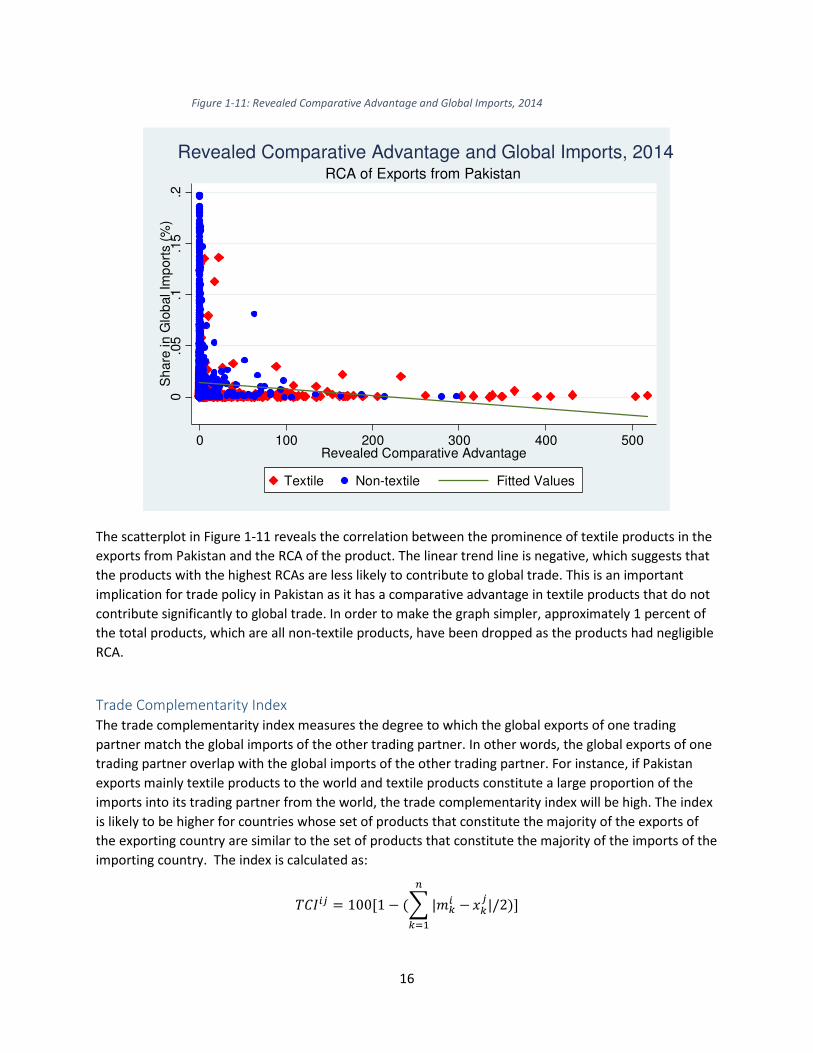
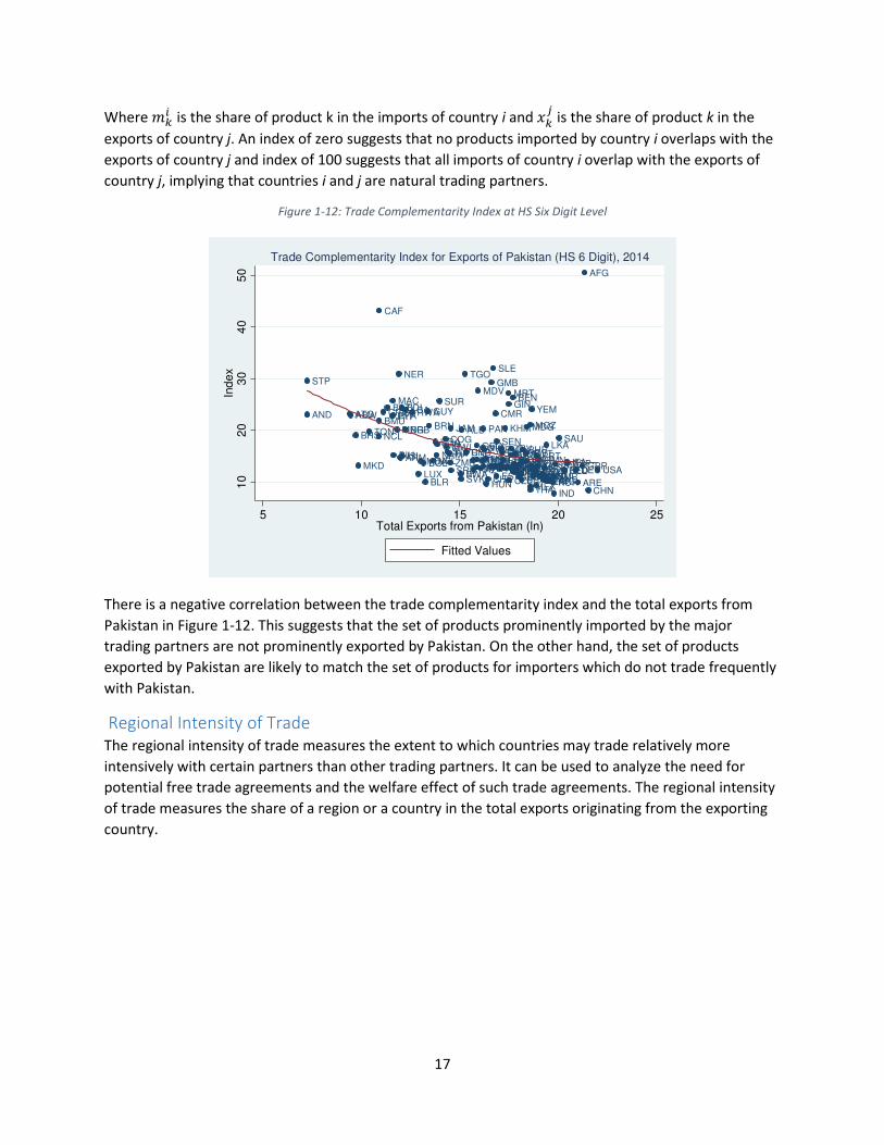
Trade Complementarity Index ............................................................................................................................. 16
Regional Intensity of Trade ...................................................................................................................................... 17
Other Important Concepts....................................................................................................................................... 19
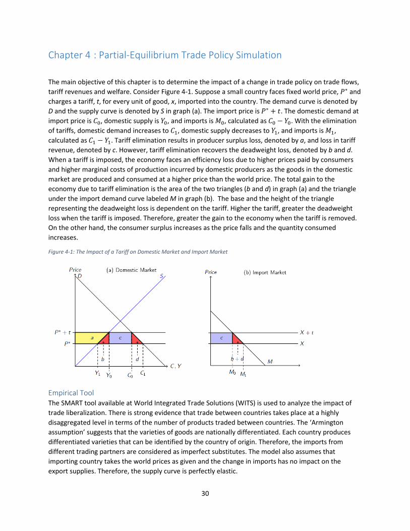
Theoretical Model ............................................................................................................................................... 31
Downloading the Data ........................................................................................................................................ 34
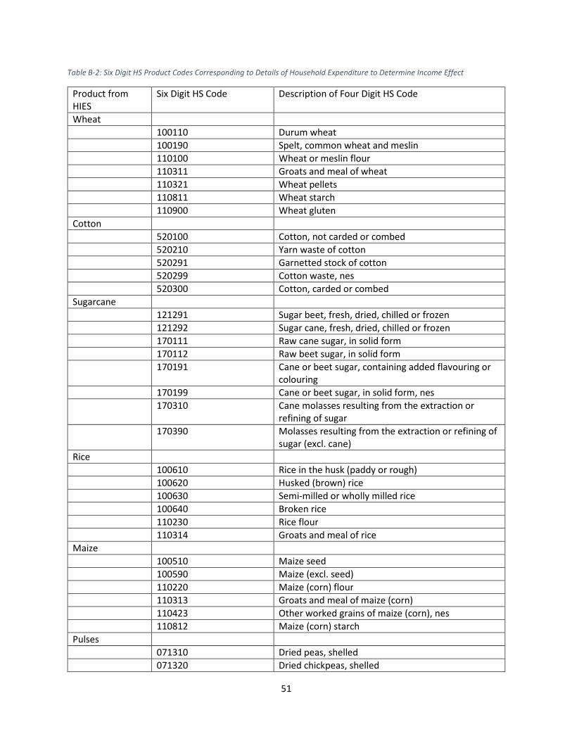
Table B-2: Six Digit HS Product Codes Corresponding to Details of Household Expenditure to Determine
Income Effect .............................................................................................................................................. 51
Figures:
Figure 1-1: Exports, Imports and Trade Openness of Pakistan ..................................................................... 4
Figure 1-2: Percentage Change in Openness and GDP per Capita, 2004-2014 ............................................. 5
Figure 1-3: Exports, Imports and Trade Openness of Pakistan, South Asian Countries and World as a
Percentage of GDP ........................................................................................................................................ 6
Figure 1-4: Percentage of Total Exports from Pakistan to its Top Ten Export Destinations in 2014 ............ 7
Figure 1-5: Percentage of Total Exports from Pakistan in Top Ten HS Sections in 2014 .............................. 8
Figure 1-6: Total Exports from Pakistan and Global Imports (By Destination) ............................................. 9
Figure 1-7: Geographical Orientation of Exports from Pakistan in 2014 ...................................................... 9
Figure 1-8: Product Orientation of Exports from Pakistan in 2014 at HS Six Digit-Level (Textile Products vs
Product Orientation of Exports from Pakistan at HS Six Digit-Level
1
23
4
5
67
8
9 1011
12
13
14
1516
17
18
19 20
21
22
05
10
15
CA
GR
in Im
port
s 2
004
-20
14
(%
)
-10 -5 0 5% Share in Total Exports (ln), 2014
Fitted Values
By HS Section
Product Orientation of Exports from Pakistan
11
The product orientation of exports from Pakistan is plotted in Figure 1-8, comparing textile to non-
textile products5. The regression line is flat, which suggests that there is no relationship between import
growth between 2004 and 2014 and the share of products in the total exports from Pakistan in 2014.
The growth rates are calculated for products that report positive exports in 2004 and 2014, while the
percentage share of exports is calculated for products that report positive exports in 2014. As expected,
majority of the products with larger share of total exports are textile products. However, when the
relationship is studied at the sectoral-level, the results in Figure 1-9 suggest a positive relationship
between the share of sectors in total exports from Pakistan and the growth in total imports between
2004 and 2014. Mineral products, vegetable products and precious metals reported the highest growth
rates in their trading values. These growth rates were likely driven by their price-levels as several
commodities reached their historical peak between 2004 and 2014.
Intra-industry Trade
The United States not only exports cars to Germany but also imports car parts from Germany. This is an
example of intra-industry trade. A large proportion of global trade takes place within the same industry,
when two countries may trade in the same product in both directions. Intra-industry trade is more likely
between countries that produce as well as consume a greater number of varieties, such as countries
with higher levels of GDP and GDP per capita. In addition, intra-industry trade is more likely between
trading partners that trade more frequently.
In order to determine the degree of intra-industry trade, the total value of products traded in both
directions (the sum of imports and exports of products that are both exported as well imported by the
two trading partners) is divided by the sum of total exports and imports between the two countries. This
formula indicates the trade overlap between two countries as it determines the ratio of bilateral trade
that flows in both directions to total bilateral trade. For instance, if Pakistan exports $100 million of
cotton yarn and imports $ 100 million of cotton yarn from China as well as imports $ 200 million of
mobile phones from China but does not export any mobile phones to China, the trade overlap will be (�������)����������� = 0.5. The numerator is the sum of products that are exported to China as well as imported
into Pakistan (two-way trade) and the denominator is the sum of total exports and imports between
Pakistan and China. The products are considered at HS six digit-level.
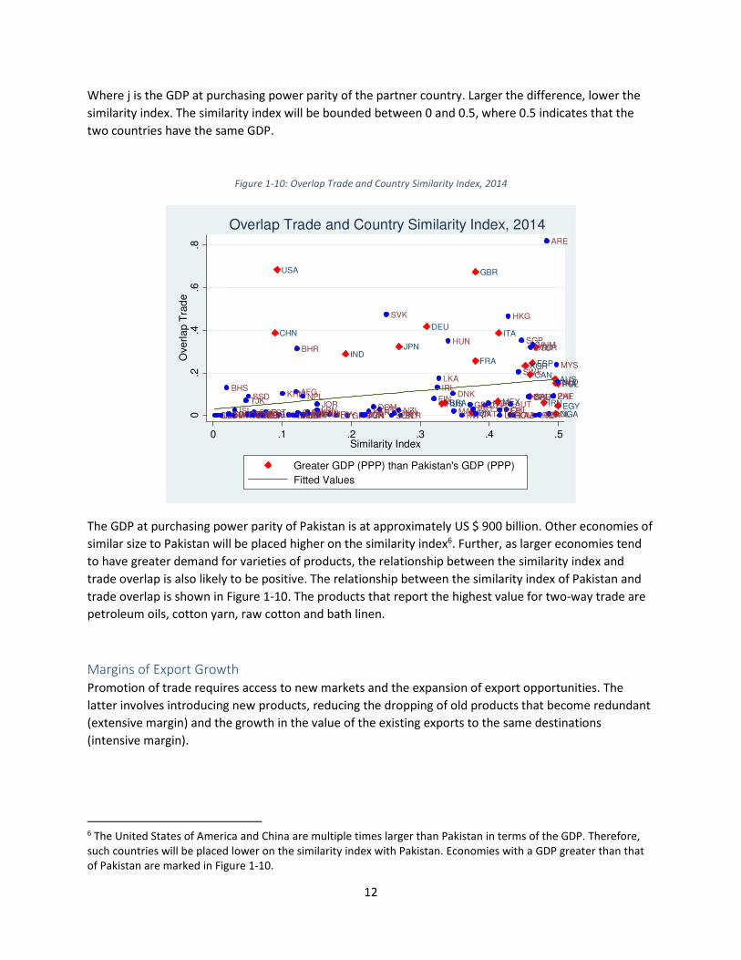
The similarity index, which is calculated as the lack of difference in the GDP between the reporting
country and the partner country, is likely to play an important role in influencing the overlapping trade
between two countries. The similarity index can be written as:
� = 1 − ������������ + �����
�− ���������� + �����
�
5 Section numbers and short title in brackets: 1 (Live Animals), 2 (Vegetable Products), 3 (Animal Fats), 4 (Prepared
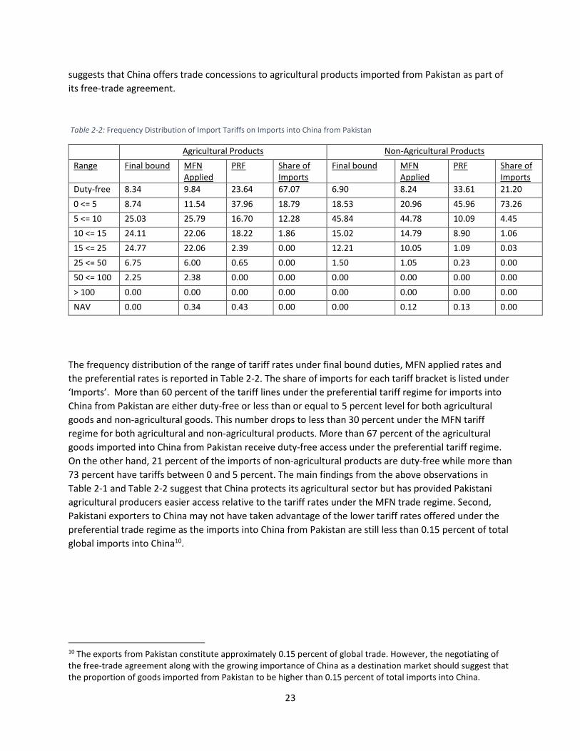
The section-wise breakup of final bound duties, MFN applied rates and preferential rates on imports
into China from Pakistan are reported in Table 2-3. The ‘duty-free share’ is the percentage of tariff lines
25
that are provided duty-free access under the respective trade regime11. The share of imports is
calculated as the percentage share of total imports into China from Pakistan in each section. The duty-
free share of imports indicates the percentage of imports that are imported into China from Pakistan
duty-free under the preferential trade regime12. China provides significant benefits to Pakistani
exporters as the share of duty-free tariffs under the preferential tariff regime is higher than the share of
duty-free tariffs under the MFN regime for majority of the HS sections.
11 The number of products reported under MFN tariffs differ from the number of products reported under PRF.
Therefore, this may give rise to the discrepancy between the percentages of tariff lines that are duty-free under
the respective trade regime. 12 More than 90 percent of the imports into China from Pakistan in mineral products, wood, and base metals is
already duty-free under the MFN applied tariff regime.
26
Chapter 3 : Analyzing Bilateral Trade Using the Gravity Equation
Gravity Equation:
The size of the bilateral flow between two countries can be estimated by the “gravity equation”.
Analogous to the Newtonian law of gravity, countries are likely to trade in proportion to their sizes and
proximity to each other. The simple gravity equation can be formulized in the following terms13:
�(� ��(4�∅(�
Where �(� is the total exports from i to j, �( comprises of exporter characteristics, 4� comprises of
importer characteristics and ∅(� represents the degree of access of exporter i into the market of
importer j.
Source:
The bilateral export flow from Pakistan to the respective trading partners is borrowed from UN
COMTRADE. The total number of export destinations with positive flows ranged from 183 in 2009 to 190
in 2014. The time period considered is from 2004 to 2014. Pakistan signed free trade agreements with
multiple trading partners as well as witnessed a doubling of its total exports during this time period. The
GDP per capita at PPP (current international dollars) and GDP at PPP (current international dollars) for
the importers are borrowed from World Development Indicators. Distance between Pakistan and the
trading partner, the dummy variables on border with Pakistan, common official language, colonizer,
common colonizer and whether the importing country is landlocked is borrowed from CEPII. Pakistan
has signed trade agreements with Sri Lanka (2005), other SAFTA countries (2006), China (2007) and
Malaysia (2008)14.
Empirical Equation:
The gravity equation can be represented by taking the natural logarithms of the variables. The exports
can be estimated using the following logarithmic equation:
67�(� 67� � 67�( � 674� � 67∅(�
The monetary value of exports, GDP of the respective countries and distance can be converted to
natural logarithmic values. However, some of the variables included are taken as dummy variables, such
as border, common official language, colonizer, common colonizer, and regional trade agreements.
These variables are included in the binary form (0 or 1). The aforementioned dummy variables tend to
lower the search costs between businesses across countries as presence in countries sharing borders,
having historical linkages and engaging in trade agreements are likely to lower their costs of business.
The regression analysis below estimates the exports from Pakistan to its trading partners based on
independent variables such as GDP of the importing country, GDP per capita of the importing country,
whether the importing county is land locked (dummy variable) and bilateral variables, such as distance,
13 Several additions to the simple gravity model have been introduced. One such addition adjusts the trade costs
between two countries using land and border characteristics such as whether countries are either landlocked or an
island or whether the two countries share a contiguous border, a common language or colonial linkages. 14 SAFTA countries include Afghanistan (acceded in 2011), Bangladesh, Bhutan, India, Maldives, Nepal, Pakistan
and Sri Lanka. The information on RTAs is available at World Trade Organization’s http://rtais.wto.org/
27
common border, common official language, trading partner as colonizer, common colonizer and the
enforcing of a regional trade agreement. Except for distance, all bilateral variables are binary dummy
variables with a value of either 1 if true or 0 if false. The analysis is conducted using simple ordinary least
squares estimation as well as Tobit and Poisson estimations.
There are several countries that do not trade with each other in a given year. The bilateral exports from
Pakistan to the trading partner will not be reported for such instances. The natural logarithmic value for
such either missing values or zeros is undefined. The values can be dropped if zeros are randomly
distributed and that the presence of zero trade flow is not informative. However, trade theory suggests
that there is substantial costs involved to participate in international trading activities and that zero
trade can indicate either or all of the following: prohibitive transportation costs, low returns to
investments in costs related to trade or relatively small size of the trading partner. Therefore, the
observation of zero trade flow is informative and the value should be included in the estimations. The
Tobit and Poisson estimations are introduced in order to account for the zero values.
The Tobit estimation is a standard method to estimate equations in which the dependent variable is
likely to consist of a larger number of zeros. As Tobit model requires some observations to be censored,
it is a plausible assumption for measuring trade flow for countries in which data may not be accurate. If
the data is accurate, the Tobit estimation may however eliminate crucial information necessary to
determine the trading patterns. The Poisson estimation avoids dropping zeros and is used to model
count data. The Poisson distribution involves a skewed, discrete distribution that includes non-negative
numbers only. The Poisson estimator determines the probability that trade occurs between the trading
partners.
The OLS is estimated using export values where zero trade values are treated as missing values after log
transformation15. However, all trade values (including zeros) are scaled by adding one before the log
transformation for the Tobit estimations. The log of trade values between countries that do not report
any trade are treated as zero in the Tobit estimations and the estimation is left-censored. As the Poisson
estimation is a count model for the number of times an event occurs, the zero trade values are included
in the estimations.
15 Approximately 6.5 percent of the observations reported for the export value are zero trade values.
28
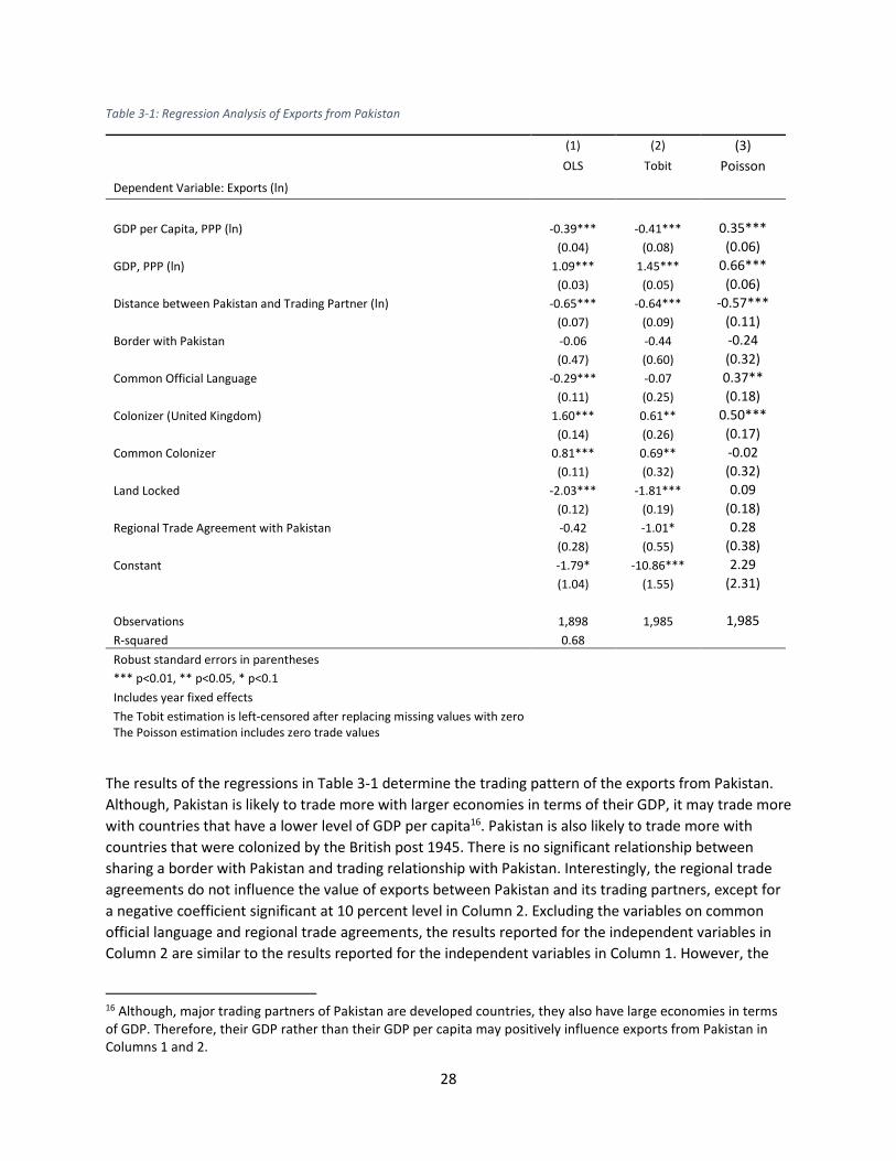
Table 3-1: Regression Analysis of Exports from Pakistan
(1) (2) (3)
OLS Tobit Poisson
Dependent Variable: Exports (ln)
GDP per Capita, PPP (ln) -0.39*** -0.41*** 0.35***
(0.04) (0.08) (0.06)
GDP, PPP (ln) 1.09*** 1.45*** 0.66***
(0.03) (0.05) (0.06)
Distance between Pakistan and Trading Partner (ln) -0.65*** -0.64*** -0.57***
(0.07) (0.09) (0.11)
Border with Pakistan -0.06 -0.44 -0.24
(0.47) (0.60) (0.32)
Common Official Language -0.29*** -0.07 0.37**
(0.11) (0.25) (0.18)
Colonizer (United Kingdom) 1.60*** 0.61** 0.50***
(0.14) (0.26) (0.17)
Common Colonizer 0.81*** 0.69** -0.02
(0.11) (0.32) (0.32)
Land Locked -2.03*** -1.81*** 0.09
(0.12) (0.19) (0.18)
Regional Trade Agreement with Pakistan -0.42 -1.01* 0.28
(0.28) (0.55) (0.38)
Constant -1.79* -10.86*** 2.29
(1.04) (1.55) (2.31)
Observations 1,898 1,985 1,985
R-squared 0.68
Robust standard errors in parentheses *** p<0.01, ** p<0.05, * p<0.1 Includes year fixed effects
The Tobit estimation is left-censored after replacing missing values with zero
The Poisson estimation includes zero trade values
The results of the regressions in Table 3-1 determine the trading pattern of the exports from Pakistan.
Although, Pakistan is likely to trade more with larger economies in terms of their GDP, it may trade more
with countries that have a lower level of GDP per capita16. Pakistan is also likely to trade more with
countries that were colonized by the British post 1945. There is no significant relationship between
sharing a border with Pakistan and trading relationship with Pakistan. Interestingly, the regional trade
agreements do not influence the value of exports between Pakistan and its trading partners, except for
a negative coefficient significant at 10 percent level in Column 2. Excluding the variables on common
official language and regional trade agreements, the results reported for the independent variables in
Column 2 are similar to the results reported for the independent variables in Column 1. However, the
16 Although, major trading partners of Pakistan are developed countries, they also have large economies in terms
of GDP. Therefore, their GDP rather than their GDP per capita may positively influence exports from Pakistan in
Columns 1 and 2.
29
Poisson estimations in Column 3 reveal certain differences. As the Poisson estimation is a count model it
estimates the impact on the count of the dependent variable due to changes in the independent
variable. The expected increase in log count of trading relationships between Pakistan and its trading
partner with an increase in one-unit of the independent variable is determined by the coefficient. As
reported in Column 3, Pakistan is more likely to report trading relationships with larger economies and
countries with higher GDP per capita as well countries with common official language and with United
Kingdom, its colonizer. It is less likely to report trading relationships with countries located at a further
distance. The Poisson distribution may seem more realistic as the effect of GDP per capita and the
common official language are positive. This is more consistent to the theoretical aspects of the gravity
Where ki is the labor income generated by the household, \i�̂ is the share of income generated by
selling tradable goods, \iJ� is the share of income generated by selling non-tradable goods, \i^l is the
share of expenditure in consumption of tradable goods and \iJl is the share of expenditure in
consumption of non-tradable goods. <\i�̂ � \i^l @ and <\iJ� � \iJl @ are the exposure of households to
changes in prices of tradable goods and non-tradable goods respectively. Larger the difference, greater
the impact of changes in prices of the respective goods and consequently, the total effect. An increase in
the tariff rates will result in ∆]^j > 0 and a decrease in the tariff rates will result in ∆]^j < 0. For
simplicity, it is assumed that the change in tariff rates has no impact on ∆]Jj and ∆[j.
Source
The data is borrowed from the Household Integrated Economic Survey (HIES) 2010-11. The HIES is a
component of the Pakistan Social and Living Standard Measurement (PSLM) Project by the Pakistan
Bureau of Statistics. The HIES collects information on several social and economic indicators of
households across provinces in Pakistan. The primary purpose of the HIES is to collect information on
39
the income and consumption patterns of households. Household characteristics such as size of family
and the employment status of household member amongst others are also collected.
Although, the data collected from the surveys is extensive and across both urban and rural areas, this
study is limited to households in the rural areas as the purpose of this study focuses on the income and
consumption effects of a change in tariff on food products. Rural households are more likely than urban
households to be consumers as well as producers of food products. The households are surveyed on
their bi-weekly expenditure on food items and the income generated from the cultivation of crops. The
per capita expenditure is calculated to measure the purchasing power of the households.
The tariff data is borrowed from World Integrated Trade Solution (WITS) available at
http://wits.worldbank.org. World average tariff rates on the imports of goods into Pakistan for 2004 and
2011 is downloaded from WITS18. The data is downloaded at six digit HS code. The HS codes are
matched to the list of products specified in HIES, provided in Appendix B, in order to determine the tariff
rates necessary to calculate the consumption effect and the income effect. The products listed in
household expenditures sheet is matched with the tariff data available from WITS at four digit HS codes
and the products listed in the household income sheet is matched with the tariff data available from
WITS at six digit HS codes.
Background on Trade Liberalization in Pakistan between 2004 and 2011
Pakistan adopted trade liberalization policies in early 2000s. The policies to lower import tariffs increase
the import of food items such as sugar, livestock and vegetables along with other commodities.
According to COMTRADE, the imports increased from US $18 billion in 2004 to US $25 billion in 2005, an
increase of almost 50 percent in one year. The imports reached US $43.5 billion in 2011. The imports of
food items included in the household expenditure survey increased from US $453 million in 2004 to US
$1.47 billion in 2011. The simple average tariff rate for all imports in 2004 was 16.64 percent and the
weighted average tariff rate was 13.01 percent. The simple average tariff rate for all imports in 2011 was
12.34 percent and the weighted average tariff rate was 9.02 percent. This suggests a drop in the tariff
rates between 2004 and 2011. Pakistan undertook policies to lower import tariffs on several goods
including food items. The income effect and the consumption effect of rural households will reflect the
results of such policies. During this period, Pakistan also negotiated and signed free trade agreements
with China, Sri Lanka and Malaysia signifying the adoption of trade liberalization in Pakistan.
Empirics
Downloading the Tariff Data and Matching with the HIES Survey Data
First, the tariff data is downloaded from WITS to calculate the changes in the import tariffs between
2004 and 2011. The tariff data is downloaded at six digit HS codes, converted to four digits HS code to
match the product codes of food items in the expenditure survey. As the import tariffs are listed at six
18 Although, it is possible that the majority of the change in the price levels between 2004 and 2011 may have
occurred in the earlier years rather than the latter years. This exercise does not discount for such a scenario. The
purpose of the exercise is to determine the simple percentage price change between 2004 and 2011. Please refer
to the section on the background for a summary analysis of import flow into Pakistan between 2004 and 2011 and
the change in tariff rates.
40
digit HS code, the tariffs are weighted at the six-digit level using import data and then summed up to the
respective product-level category in the HIES.
The HS codes are maintained at six digit-level to match the products listed in the income survey and
subsequently calculate the income effect. The trade-weighted import tariffs for each product code
reported in HIES are calculated using the collapse function in STATA by assigning import values as
weights for the respective tariffs.
Calculating the Change in Weighted Tariff Rates
Next, the weighted tariffs for 2004 and 2011 are used to calculate the change in price levels19. The
following formula is used to calculate the change in tariff rates, ∆`(,����p����, ∆ �̀,����p����:20
∆`(,����p���� = 100 + `(,����100 + `(,���� − 1
∆ �̀,����p���� = 100 + �̀,����100 + �̀,���� − 1
where each product group in the household bi-weekly expenditure survey is denoted by i, and each
product group in the household income survey is denoted by j21. `(,���� is the weighted average tariff
rates for the products listed in the household surveys in 2004 and `(,���� is the weighted average tariff
rates for the products listed in the household surveys in 2011.
The level of expenditure incurred and the level of income earned in 2004 for the consumption and the
production respectively of the same bundle of goods as in 2011 will be higher if the prices of the
tradable goods decrease between 2004 and 2011. The consumption effect is the impact of trade policies
on household expenditures through the prices of goods consumed by the household. The income effect
is the impact of trade policies on household income through the prices of goods produced by the
household. Theoretically, a reduction in the prices of goods will lead to a positive consumption effect
and a negative income effect.
The change in weighted average tariff is multiplied by the share in expenditure of each product group in
total expenditure on food products22. The resultant value is the change in the share in expenditure of
each product group. Therefore, an increase in the total share implies that the households are incurring
greater expenditure on food products in order to remain at the same utility level in the base year, 2011.
This is the case if the prices of a product are higher in 2004 than in 2011, our base year for the survey
19 The household surveys were conducted in 2011. Therefore, all percentage changes have been calculated taking
2011 as the base year. A lower tariff rate in 2011 than 2004 will imply a fall in prices between 2004 and 2011.
Therefore, the consumption effect will be positive and the income effect will be negative for a tariff rate that is
lower in 2011 than in 2004. 20 As the product groups are classified differently in the household expenditure sheet and the household income
sheet, different notations have been adopted to denote the product groups across the two sheets. 21 Bi-weekly expenditures can be scaled up to annual expenditures. The shares in bi-weekly expenditures will be
the same as in annual expenditures. 22 For simplicity, only the food products are classified as tradable goods. All the remaining products are classified as
non-tradable goods.
41
data. The summation of this across all product groups will provide the value of the consumption effect.
Tariff liberalization will have a positive impact on the consumption effect. A similar inference can be
made for the income effect.
Calculating the Consumption Effect
The change in share of expenditure on food products at the household-level between 2004 and 2011, \i(,����lq/r , is calculated by multiplying the change in weighted tariff between 2004 and 2011, as
formulated above, with the share of expenditure on food items incurred for each of the nine product
groups of tradable goods listed in the bi-weekly household expenditure sheet in 2011:
\i(,����lq/r = ∆`(,����p���� ∗ (\i(,����l ) The consumption effect at the household level is then calculated as the summation of the change in share
of all food products purchased between 2004 and 2011, where i=1,2,……,T:
\i^,����lq/r = ∑ \i(,����lq/r(̂0�
The total consumption effect in the economy across all households in the rural areas is the summation
of all the values calculated at the household level.
Calculating the Income Effect
After calculating the consumption effect, the next step is to determine the income effect. The change in
share of income generated by cultivating and selling tradable products between 2004 and 2011, \i�,�����jqR
, is the income share of that product sold in 2011 multiplied by the change in weighted tariff for the
respective product between 2004 and 2011.
\i�,�����jqR = ∆ �̀,����p���� ∗ (\i�,����
� )
The income effect at the household level is calculated as the summation of the change in share of all
tradable products sold between 2004 and 2011, where where j=1,2,……,T: :
\i^,�����jqR = ∑ \i�,�����jqR�̂0�
The total effect for a household from a reduction in price of tradable goods between 2004 and 2011 is:
\i^,����^qT \i^,����lq/r � \i^,�����jqR
where the consumption effect and the income effect have opposite signs.
The per capita annual expenditure is calculated as the total annual expenditure incurred by a household
divided by the total number of individuals in the households. The consumption effect and the income
effect are plotted against per capita annual expenditure incurred by a household in order to capture the
42
purchasing power of a household with respect to the number of individuals belonging to a household. A
richer household will have a greater purchasing power. If government policies favorably redistribute
income, the consumption effect of a decrease in price should be higher for the poorer households and
the income effect of a decrease in price should be smaller for poorer households.
As the number of households surveyed is substantially lower than the number of households actually
present within each primary sampling unit, a sampling weight is assigned to each primary sampling unit
in order to determine the actual size of the primary sampling unit with respect to the number of
households surveyed. The weight determines the probability that the household will be selected. If the
household has a high probability of being selected, then the household will be over-represented in the
survey, and a lower weight will be assigned to a household. The weights used in the study are provided
in the HIES data.
43
Results
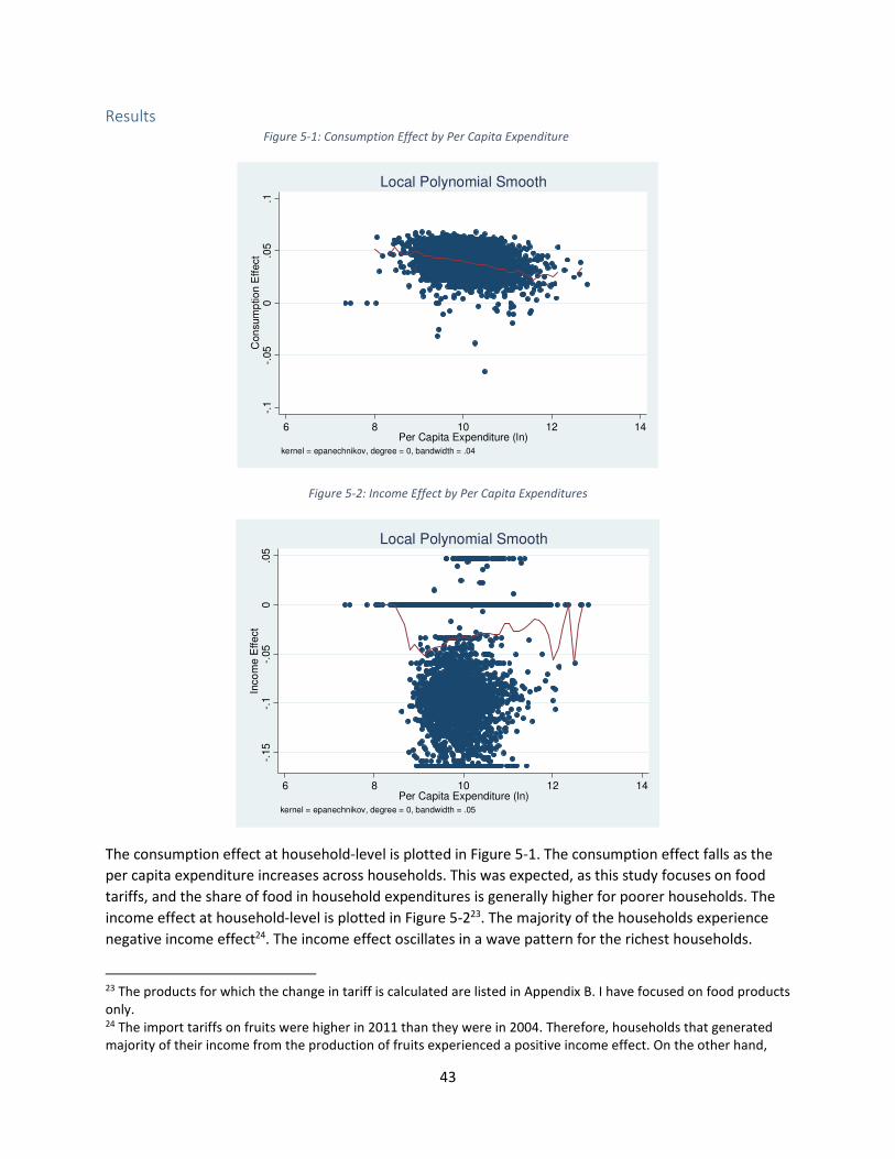
Figure 5-1: Consumption Effect by Per Capita Expenditure
Figure 5-2: Income Effect by Per Capita Expenditures
The consumption effect at household-level is plotted in Figure 5-1. The consumption effect falls as the
per capita expenditure increases across households. This was expected, as this study focuses on food
tariffs, and the share of food in household expenditures is generally higher for poorer households. The
income effect at household-level is plotted in Figure 5-223. The majority of the households experience
negative income effect24. The income effect oscillates in a wave pattern for the richest households.
23 The products for which the change in tariff is calculated are listed in Appendix B. I have focused on food products
only. 24 The import tariffs on fruits were higher in 2011 than they were in 2004. Therefore, households that generated
majority of their income from the production of fruits experienced a positive income effect. On the other hand,
The weighted average tariff rates on the product group defined as fruits is greater in 2011 than in 2004.
Therefore, the prices of fruits has increased during the time period. This suggests a positive income
effect for households that earn a larger proportion of their income by cultivating fruits.
Table 5-1: Income, Consumption and Overall Effects by Deciles
Decile Income Effect Consumption
Effect
Total Effect
1 -0.044 0.045 0.001
2 -0.043 0.043 0.000
3 -0.033 0.042 0.009
4 -0.036 0.041 0.005
5 -0.034 0.041 0.007
6 -0.031 0.040 0.009
7 -0.035 0.039 0.004
8 -0.032 0.038 0.006
9 -0.028 0.036 0.007
10 -0.026 0.032 0.006
The total effect by decile of per capita expenditure is listed in Table 5-1. The poorest households in the
rural areas experience the smallest total effect as the larger positive consumption effect is canceled by
the negative income effect, which is similar in magnitude. The consumption effect falls as the level of
per capita expenditure by households increase. However, the income effect is oscillatory across the per
capita expenditure incurred by households. Although, the poorest households face lower total effect
than the richest households in the rural areas, the households belonging to the middle deciles of per
capita expenditure levels benefit the most in terms of total effect than the households in the two
extremes of per capita expenditure levels.
wheat reported the highest change in tariff rates between 2004 and 2011. Households concentrated towards the
bottom of the graph, below -0.15, are likely to generate income predominantly from wheat.
45
Figure 5-3: Total Effect by Provinces
The box plot for the total effects by provinces is shown in Figure 5-3. The lower and the upper edges of
the boxes display the 25th and the 75th percentile of the rural households respectively, the horizontal line
within the box displays the 50th percentile and the upper horizontal line above the boxes display the 95th
and below the boxes display the 5th percentile of the rural households in the respective provinces. The
outliers are represented by dots. The box plot shows that more than 50 percent of the rural households
will gain from trade liberalization across all provinces. Only the outliers will lose in Balochistan due to
trade liberalization, suggesting that only an insignificant proportion of households in the province lose
from trade liberalization. It is also interesting to note that the gap between the respective percentile
identifiers is spread out for the lower percentiles than for the upper percentiles. This suggests that there
is lower dispersion in the total effect amongst households that report higher levels of gain in total
effect25.
In order to determine whether the removal of a tariff has a progressive or a ‘pro-poor’ bias, that is it
benefits the poor households more than the richer households, it is important to quantify the impact of
tariffs and tariff changes on different income levels based on either the quantiles, deciles or centiles of
income. This can be achieved by performing the Locally Weighted Scatterplot Smoothing (LOWESS
estimation in STATA).
25 A deeper analysis, for instance using population weights and GDP weights for provinces, is necessary to obtain a
better understanding of the distribution of the total effect across provinces. Such an exercise is beyond the scope
of this project.
-.15
-.1
-.05
0.0
5.1
Tota
l E
ffe
ct
Balochistan KP (NWFP) Punjab Sindh
46
Figure 5-4: Tariff and Change in Tariff Sorted on Income Distribution
The consumption-weighted average tariffs and average change in tariffs are calculated on the basis of
the weight of the products (food items) consumed by the households. The total income earned by the
households is distributed based on centiles. Sampling weights provided in the survey data are used. The
lowess smoother curves are plotted in Figure 5-4. The richer households faced higher tariff rates than
the poorer households. Further, the reduction in the tariff rates between 2004 and 2011 was ‘pro-poor’
as the change had a greater impact on the consumption bundle of the poorer households than the
richer households.
78
910
11
12
(Mean)
Tariff, 2011
0 20 40 60 80 100100 quantiles of income
bandwidth = .8
Lowess smoother
3.5
44.5
55.5
(Mean)
Perc
enta
ge C
hange in T
ari
ff, 2004-2
011
0 20 40 60 80 100100 quantiles of income
bandwidth = .8
Lowess smoother
47
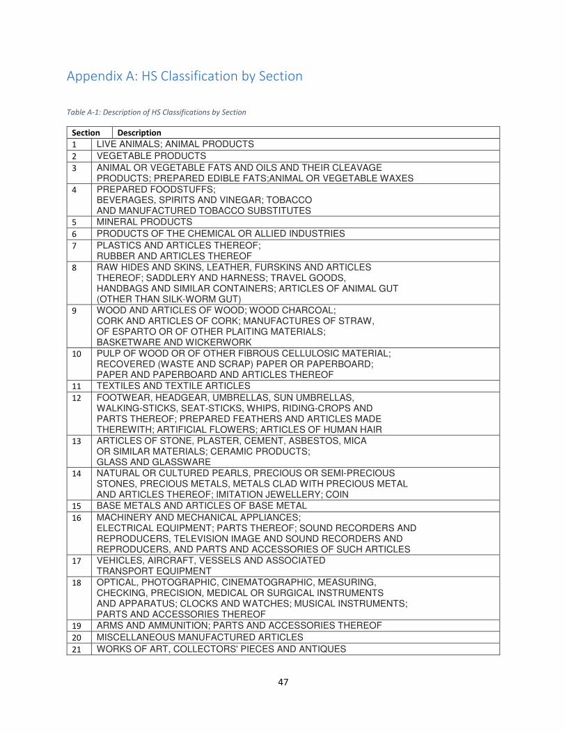
Appendix A: HS Classification by Section
Table A-1: Description of HS Classifications by Section
Section Description
1 LIVE ANIMALS; ANIMAL PRODUCTS
2 VEGETABLE PRODUCTS
3 ANIMAL OR VEGETABLE FATS AND OILS AND THEIR CLEAVAGE PRODUCTS; PREPARED EDIBLE FATS;ANIMAL OR VEGETABLE WAXES
4 PREPARED FOODSTUFFS; BEVERAGES, SPIRITS AND VINEGAR; TOBACCO AND MANUFACTURED TOBACCO SUBSTITUTES
5 MINERAL PRODUCTS
6 PRODUCTS OF THE CHEMICAL OR ALLIED INDUSTRIES
7 PLASTICS AND ARTICLES THEREOF; RUBBER AND ARTICLES THEREOF
8 RAW HIDES AND SKINS, LEATHER, FURSKINS AND ARTICLES THEREOF; SADDLERY AND HARNESS; TRAVEL GOODS, HANDBAGS AND SIMILAR CONTAINERS; ARTICLES OF ANIMAL GUT (OTHER THAN SILK-WORM GUT)
9 WOOD AND ARTICLES OF WOOD; WOOD CHARCOAL; CORK AND ARTICLES OF CORK; MANUFACTURES OF STRAW, OF ESPARTO OR OF OTHER PLAITING MATERIALS; BASKETWARE AND WICKERWORK
10 PULP OF WOOD OR OF OTHER FIBROUS CELLULOSIC MATERIAL; RECOVERED (WASTE AND SCRAP) PAPER OR PAPERBOARD; PAPER AND PAPERBOARD AND ARTICLES THEREOF
11 TEXTILES AND TEXTILE ARTICLES
12 FOOTWEAR, HEADGEAR, UMBRELLAS, SUN UMBRELLAS, WALKING-STICKS, SEAT-STICKS, WHIPS, RIDING-CROPS AND PARTS THEREOF; PREPARED FEATHERS AND ARTICLES MADE THEREWITH; ARTIFICIAL FLOWERS; ARTICLES OF HUMAN HAIR
13 ARTICLES OF STONE, PLASTER, CEMENT, ASBESTOS, MICA OR SIMILAR MATERIALS; CERAMIC PRODUCTS; GLASS AND GLASSWARE
14 NATURAL OR CULTURED PEARLS, PRECIOUS OR SEMI-PRECIOUS STONES, PRECIOUS METALS, METALS CLAD WITH PRECIOUS METAL AND ARTICLES THEREOF; IMITATION JEWELLERY; COIN
15 BASE METALS AND ARTICLES OF BASE METAL
16 MACHINERY AND MECHANICAL APPLIANCES; ELECTRICAL EQUIPMENT; PARTS THEREOF; SOUND RECORDERS AND REPRODUCERS, TELEVISION IMAGE AND SOUND RECORDERS AND REPRODUCERS, AND PARTS AND ACCESSORIES OF SUCH ARTICLES
17 VEHICLES, AIRCRAFT, VESSELS AND ASSOCIATED TRANSPORT EQUIPMENT
18 OPTICAL, PHOTOGRAPHIC, CINEMATOGRAPHIC, MEASURING, CHECKING, PRECISION, MEDICAL OR SURGICAL INSTRUMENTS AND APPARATUS; CLOCKS AND WATCHES; MUSICAL INSTRUMENTS; PARTS AND ACCESSORIES THEREOF
19 ARMS AND AMMUNITION; PARTS AND ACCESSORIES THEREOF
20 MISCELLANEOUS MANUFACTURED ARTICLES
21 WORKS OF ART, COLLECTORS' PIECES AND ANTIQUES
48
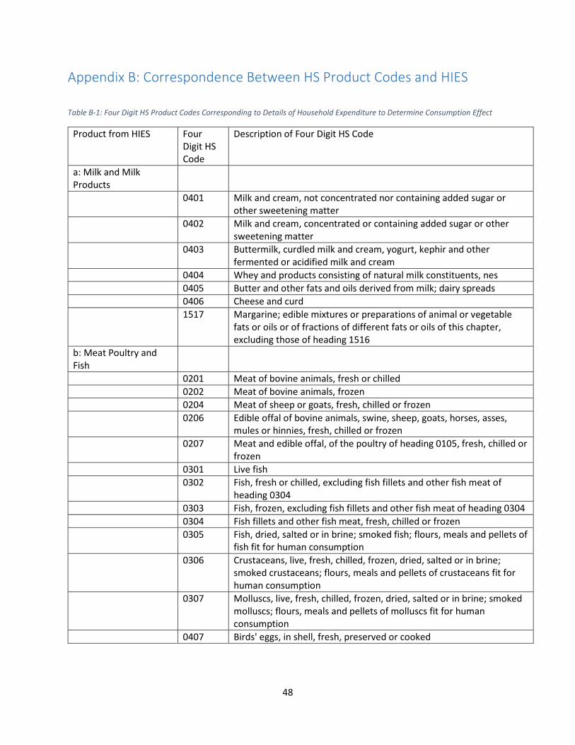
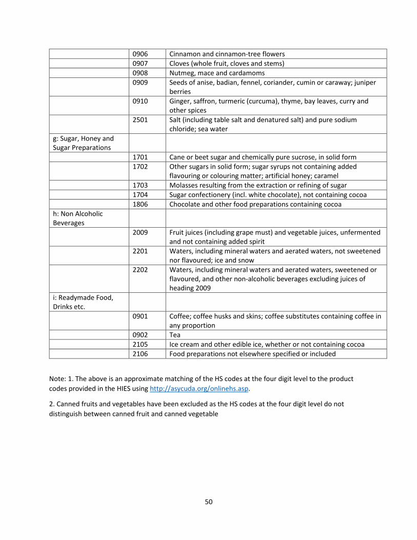
Appendix B: Correspondence Between HS Product Codes and HIES
Table B-1: Four Digit HS Product Codes Corresponding to Details of Household Expenditure to Determine Consumption Effect
Product from HIES Four
Digit HS
Code
Description of Four Digit HS Code
a: Milk and Milk
Products
0401 Milk and cream, not concentrated nor containing added sugar or
other sweetening matter
0402 Milk and cream, concentrated or containing added sugar or other
sweetening matter
0403 Buttermilk, curdled milk and cream, yogurt, kephir and other
fermented or acidified milk and cream
0404 Whey and products consisting of natural milk constituents, nes
0405 Butter and other fats and oils derived from milk; dairy spreads
0406 Cheese and curd
1517 Margarine; edible mixtures or preparations of animal or vegetable
fats or oils or of fractions of different fats or oils of this chapter,
excluding those of heading 1516
b: Meat Poultry and
Fish
0201 Meat of bovine animals, fresh or chilled
0202 Meat of bovine animals, frozen
0204 Meat of sheep or goats, fresh, chilled or frozen


![JD Edwards EnterpriseOne Applications Localizations for … · 2020-06-11 · [1]JD Edwards EnterpriseOne Applications Localizations for Australia and Singapore Implementation Guide](https://static.documents.pub/doc/80x56/5f3196ce7cc95632a0421491/jd-edwards-enterpriseone-applications-localizations-for-2020-06-11-1jd-edwards.jpg)


![JD Edwards EnterpriseOne Applications Localizations for ... · [1]JD Edwards EnterpriseOne Applications Localizations for Portugal Implementation Guide Release 9.1 E23360-09 February](https://static.documents.pub/doc/80x56/5e5ae6c17374176a324da0df/jd-edwards-enterpriseone-applications-localizations-for-1jd-edwards-enterpriseone.jpg)


