A Practical Quantum Instruction Set Architecture Robert S. Smith, Michael J. Curtis, William J. Zeng Rigetti Computing 775 Heinz Ave. Berkeley, California 94710 Email: {robert, spike, will}@rigetti.com Copyright c 2016 Rigetti & Co., Inc.—v2.0.20170217 Abstract —We introduce an abstract machine archi- tecture for classical/quantum computations—including compilation—along with a quantum instruction lan- guage called Quil for explicitly writing these computa- tions. With this formalism, we discuss concrete imple- mentations of the machine and non-trivial algorithms targeting them. The introduction of this machine dove- tails with ongoing development of quantum computing technology, and makes possible portable descriptions of recent classical/quantum algorithms. Keywords— quantum computing, software architecture Contents I Introduction 1 II The Quantum Abstract Machine 2 II-A Qubit Semantics ............ 2 II-B Quantum Gate Semantics ....... 3 II-C Measurement Semantics ........ 4 III Quil: a Quantum Instruction Language 5 III-A Classical Addresses and Qubits .... 5 III-B Numerical Interpretation of Classical Memory Segments ........... 5 III-C Static and Parametric Gates ..... 5 III-D Gate Definitions ............ 6 III-E Circuits ................. 6 III-F Measurement .............. 6 III-G Program Control ............ 7 III-H Zeroing the Quantum State ...... 7 III-I Classical/Quantum Synchronization . 7 III-J Classical Instructions ......... 7 III-J1 Classical Unary Instructions 8 III-J2 Classical Binary Instructions 8 III-K The No-Operation Instruction .... 8 III-L File Inclusion Semantics ....... 8 III-M Pragma Support ............ 8 III-N The Standard Gates .......... 9 IV Quil Examples 9 IV-A Quantum Fourier Transform ..... 9 IV-B Variational Quantum Eigensolver .. 9 IV-B1 Static Implementation . . . 9 IV-B2 Dynamic Implementation . 10 V Forest: A Quantum Programming Toolkit 10 V-A Overview ................ 10 V-B Applications and Tools ........ 11 V-C Quil Manipulation ........... 11 V-D Compilation .............. 11 V-E Instruction Parallelism ........ 12 V-F Rigetti Quantum Virtual Machine . . 12 VI Conclusion 13 VII Acknowledgements 13 Appendix 13 A The Standard Gate Set ........ 13 B Prior Work ............... 13 B1 Embedded Domain- Specific Languages ..... 13 B2 High-Level QPLs ...... 13 B3 Low-Level Quantum Inter- mediate Representations . . 14 I. Introduction The underlying hardware for quantum computing has advanced rapidly in recent years. Superconducting chips with 4–9 qubits have been demonstrated with the perfor- mance required to run quantum simulation algorithms [1, 2, 3], quantum machine learning [4], and quantum error correction benchmarks [5, 6, 7]. Hybrid classical/quantum algorithms—including vari- ational quantum eigensolvers [8, 9, 10], correlated mate- rial simulations [11], and approximate optimization [12]— have much promise in reducing the overhead required arXiv:1608.03355v2 [quant-ph] 17 Feb 2017
Transcript
A Practical Quantum Instruction Set Architecture
Robert S. Smith, Michael J. Curtis, William J. ZengRigetti Computing
Abstract—We introduce an abstract machine archi-tecture for classical/quantum computations—includingcompilation—along with a quantum instruction lan-guage called Quil for explicitly writing these computa-tions. With this formalism, we discuss concrete imple-mentations of the machine and non-trivial algorithmstargeting them. The introduction of this machine dove-tails with ongoing development of quantum computingtechnology, and makes possible portable descriptionsof recent classical/quantum algorithms. Keywords—quantum computing, software architecture
The underlying hardware for quantum computing hasadvanced rapidly in recent years. Superconducting chipswith 4–9 qubits have been demonstrated with the perfor-mance required to run quantum simulation algorithms [1,2, 3], quantum machine learning [4], and quantum errorcorrection benchmarks [5, 6, 7].
Hybrid classical/quantum algorithms—including vari-ational quantum eigensolvers [8, 9, 10], correlated mate-rial simulations [11], and approximate optimization [12]—have much promise in reducing the overhead required
arX
iv:1
608.
0335
5v2
[qu
ant-
ph]
17
Feb
2017
Classical Computation Quantum Computation
Clas
sica
l Dat
a
Fig. 1. A classical/quantum feedback loop.
for valuable applications. In machine learning and quan-tum simulation, particularly for catalysts [13] and high-temperature superconductivity [9], scalable quantum com-puters promise performance unrivaled by classical super-computers.
The promise of hardware and applications must bematched with advances in programming architectures. Thedemands of practical algorithm design, as well as theshift to hybrid classical/quantum algorithms, necessitatean update to the quantum Turing machine model [14].We need new frameworks for quantum program compila-tion [15, 16, 17, 18, 19] and emulation [20, 21]. For moredetails on prior work and its relationship to the topicsintroduced here, we refer the reader to Appendix B.
These classical/quantum algorithms require a classicalcomputer and quantum computer to communicate andwork cooperatively, as in Figure 1. Within the presentedframework, classical information is fed back via a definedmemory model, which can be implemented efficiently inboth hardware and software.
In this paper, we describe an abstract machine whichserves as a model for hybrid classical/quantum computa-tion. Alongside this, we describe an instruction languagefor this machine called Quil and its suitability for programanalysis and compilation. Together these form a quantuminstruction set architecture (ISA). Lastly, we givevarious examples of algorithms in Quil, and discuss anexecutable implementation.
II. The Quantum Abstract Machine
Turing machines provide a vehicle for studying impor-tant concepts in computer science such as complexity andcomputational equivalence. While theoretically important,they do not provide a foundation for the constructionof practical computing machines. Instead, specialized ab-stract machines are designed to accomplish real-worldtasks, like arithmetic, efficiently while maintaining Turingcompleteness. These machines are often specified in theform of an instruction set architecture. Quantum Turingmachines lie in the same vein as its classical counterpart,and we follow a similar approach in the creation of apractical quantum analog.
The Quantum Abstract Machine (QAM) is an ab-stract representation of a general-purpose quantum com-puting device. It includes support for manipulating bothclassical and quantum state. The QAM executes programsrepresented in a quantum instruction language called Quil,which has well-defined semantics in the context of theQAM.
The state of the QAM is specified by the followingelements:
• A fixed but arbitrary number of qubits Nq indexedfrom 0 to Nq − 1. The kth qubit is written Qk. Thestate of these qubits is written |Ψ〉 and is initializedto |00 . . . 0〉. The semantics of the qubits are describedin Section II-A.
• A classical memory C of Nc bits, initialized to zeroand indexed from 0 to Nc − 1. The kth bit is writtenC[k].
• A fixed but arbitrary list of static gates G, and a fixedbut arbitrary list of parametric gates G′. These termsare defined in Section III-C.
• A fixed but arbitrary sequence of Quil instructions P .These instructions will be described in Section III.
• An integer program counter 0 ≤ κ ≤ |P | indicatingposition of the next instruction to execute when κ 6=|P | or a halted program when κ = |P |.
The 6-tuple (|Ψ〉 , C,G,G′, P, κ) summarizes the state ofthe QAM.
The QAM may be implemented either classically or onquantum hardware. A classical implementation is called aQuantum Virtual Machine (QVM). We describe onesuch implementation in Section V-F. An implementationon quantum hardware is called a Quantum ProcessingUnit (QPU).
The semantics of the quantum state and operationson it are described in the language of tensor products ofHilbert spaces and linear maps between them. The follow-ing subsections give these semantics in meticulous detail.Readers with intuition about these topics are encouragedto skip to Section III for a description of Quil.
A. Qubit Semantics
A finite-dimensional Hilbert space over the complexnumbers C is denoted by H . The state space of a qubit isa two-dimensional Hilbert space over C and is denoted byB. Each of these Hilbert spaces is equipped with a chosenorthonormal basis and indexing map on that basis. Anindexing map is a bijective function that maps elementsof a finite set Σ to the set of non-negative integers below|Σ|, denoted [|Σ|]. For a Hilbert space spanned by {|u〉 , |v〉}with an indexing map defined by |u〉 7→ 0 and |v〉 7→ 1, wewrite |0〉 := |u〉 and |1〉 := |v〉.
In the context of the QAM, each qubit Qk in isolationhas a state space Bk spanned by an orthonormal basis{|0〉k , |1〉k} called the computational basis. Since qubitscan entangle, the state space of the system of all qubits isnot a direct product of each constituent space, but rathera rightward tensor product
|Ψ〉 ∈H :=Nq−1⊗k=0
BNq−k−1. (1)
The meaning of the tensor product is as follows. Let |p〉i bethe pth basis vector of Hi according to its indexing map.
The tensor product of two Hilbert spaces is then
Hi⊗Hj :={ ∑p∈[dim Hi]q∈[dim Hj ]
Cp,q |p〉i ⊗ |q〉j︸ ︷︷ ︸basis element
: C ∈ Cdim Hi×dim Hj
}.
(2)The resulting basis elements are ordered by way of thelexicographic indexing map
|p〉i ⊗ |q〉j 7→ q + p dim Hj . (3)
Having the basis elements of the Hilbert space Hi “domi-nate” the indexing map is a convention due to the standarddefinition of the Kronecker product, in which for matricesA and B, A ⊗ B is a block matrix (A ⊗ B)i,j = Ai,jB.This convention, while standard, somewhat muddles thesemantics below with busy-looking variable indexes whichcount down, not up.
A basis element of H
|bNq−1〉Nq−1 ⊗ · · · ⊗ |b1〉1 ⊗ |b0〉0
can be written shorthand in bit string notation
|bNq−1 . . . b1b0〉 .
This has the particularly useful property that the bit stringcorresponds to the binary representation of the index ofthat basis element. For clarity, however, we will not usethis notation elsewhere in this paper.Example 1. A two-qubit system in the Hilbert space B2⊗B1 has the lexicographic indexing map defined by
The standard Bell state in this system is represented by theelement in the tensor space with the matrix
C = 1√2
(1 00 1
).
Eqs. (1) and (2) imply that dim H = 2Nq , and as such,|Ψ〉 can be represented as a complex vector of that length.
B. Quantum Gate Semantics
The quantum state of the system evolves by applying asequence of operators called quantum gates. Most gener-ally, these are complex unitary matrices of size 2Nq × 2Nq ,written succinctly as U(2Nq ). However, quantum gatesare typically abbreviated as one- or two-qubit unitarymatrices, and go through a process of “tensoring up” beforeapplication to the quantum state.Example 2. The Hadamard gate on Qk is defined as
H := 1√2
(1 11 −1
): Bk → Bk.
This is unitary because HH† = Ik is the identity map onBk.
The controlled-X or controlled-not gate with controlqubit Qj and target qubit Qk is defined as
CNOT :=
1 0 0 00 1 0 00 0 0 10 0 1 0
: Bj ⊗Bk → Bj ⊗Bk.
This gate is common for constructing entanglement in aquantum system.
It turns out that many different sets of these one-and two-qubit gates are sufficient for universal quantumcomputation, i.e., a discrete set of gates can be usedto approximate any unitary matrix to arbitrary accu-racy [22, 23]. In fact almost any two-qubit quantum gatecan be shown to be universal [24]. Delving into differentuniversal gate sets is beyond the scope of this work andwe refer the reader to [23] as a general reference.
We now wish to provide a constructive method forinterpreting operators on a portion of a Hilbert space asoperators on the Hilbert space itself. In the simplest case,we have a one-qubit gate U acting on qubit Qk, whichinduces an operator U on H by tensor-multiplying withthe identity map a total of Nq − 1 times:
U = INq−1 ⊗ · · · ⊗ U︸︷︷︸(Nq − k − 1)th position (zero-based)
⊗ · · · ⊗ I1 ⊗ I0. (4)
We refer to this process as lifting and reserve the tildeover the operator name to indicate such.Example 3. Consider a system of four qubits and con-sider a Hadamard gate acting on Q2. Lifting this operatoraccording to (4) gives
H = I3 ⊗ H⊗ I1 ⊗ I0.
A two-qubit gate acting on adjacent Hilbert spaces isjust as simple. An operator U : Bk ⊗Bk−1 → Bk ⊗Bk−1is lifted as
U = INq−1 ⊗ · · · ⊗ U ⊗ · · · ⊗ I1 ⊗ I0︸ ︷︷ ︸Nq − 1 factors, U at position Nq − k − 1
. (5)
However, when the Hilbert spaces are not adjacent, lift-ing involves a bit more bookkeeping because there is noobvious place to tensor-multiply the identity maps of theHilbert spaces indexed between j and k. We can resolvethis by suitably rearranging the space. We need two tools:a method to “reorganize” an operator’s action on a tensorproduct of Hilbert spaces and isomorphisms between theseHilbert spaces. The general principle to be employed isto find some operator π : H → H which acts as apermutation operator on H , and to compute π−1U ′π,where U ′ is isomorphic to U . Simply speaking, π is atemporary re-indexing of basis vectors and U ′ is just atrivial reinterpretation of U .
To reorganize, we use the fact that any permutation canbe decomposed into adjacent transpositions. For swapping
two qubits, consider the gate
SWAPj,k :=
1 0 0 00 0 1 00 1 0 00 0 0 1
: Bj ⊗Bk → Bj ⊗Bk. (6)
This is a permutation matrix which maps the basis ele-ments according to
and mapping the others identically. For adjacent transpo-sitions in the full Hilbert space, this can be trivially lifted:
τi := SWAPi,i+1 lifted by way of (5). (7)
We will use a sequence of these operators to arrange forBj and Bk to be adjacent by moving one of them nextto the other. There are two cases we need to be concernedabout: j > k and j < k.
For the j > k case, we want to map the state of Bk toBj−1. This is accomplished with the operator1
πj,k :=j−2∏i=k
τj+k−i−2,
where the product right-multiplies and is empty when k ≥j − 1.
For the j < k case, we want to map the state of Bj toBk−1, and then swap Bk−1 with Bk. We can do this withthe π operator succinctly:
π′j,k := τk−1πk,j .
Note the order of j and k in the π factor.Lastly, for the purpose of correctness, we need to
construct a trivial isomorphism
f : Bj ⊗Bk → Bj ⊗Bj−1, (8)
which is defined as the bijection between basis vectors withthe same index.
Now we may consider two-qubit gates in their fullgenerality. Let U : Bj ⊗Bk → Bj ⊗Bk be the gate underconsideration. Perform a “change of coordinates” on U todefine
V := fUf−1 : Bj ⊗Bj−1 → Bj ⊗Bj−1,
and lift V to V : H →H by way of (5). Then the liftedU can be constructed as follows:
U ={π−1j,k V πj,k if j > k, and
(π′j,k)−1V π′j,k if j < k.(9)
Since the π operators are essentially compositions of invo-lutive SWAP gates, their inverses are just reversals.
With care, the essence of this method generalizesaccordingly for gates acting on an arbitrary number ofqubits.
1This is an example of the effects of following the Kroneckerconvention. This product is really just “τi in reverse.”
We end this section with an example of a universalQAM.Example 4. Define all possible liftings of U within H as
L(U) := {U lifted for all qubit permutations}.
Define the gates S := ( 1 00 i ) and T :=
( 1 00 eiπ/4
). A QAM
with2
G = L(H) ∪ L(S) ∪ L(T) ∪ L(CNOT) and G′ = {}
can compute to arbitrary accuracy the action of any Nq-qubit gate, possibly with P exponential in length. See [23,§4.5] for details.
C. Measurement Semantics
Measurement is a surjective-only operation and is non-deterministic. In the space of a single qubit Qk, thereare two outcomes to a measurement. The outcomes aredetermined by lifting and applying—up to a scalar factor—either of the measurement operators3
Mk0 := |0〉k 〈0|k and Mk
1 := |1〉k 〈1|k
to the quantum state. These can be interpreted as projec-tions onto either of the basis elements of the Hilbert space.More generally, in any finite Hilbert space H , we have theset of measurement operators
M(H ) :={|v〉 〈v| : |v〉 ∈ basis H
}.
In the QAM, when a qubit is measured, a particularmeasurement operator µ is selected and applied accordingto the probability
P (µ) := P (µ is applied during meas.) = 〈Ψ| µ†µ |Ψ〉 .(10)
Upon selection of an operator, the quantum state trans-forms according to
|Ψ〉 ← 1P (µ) µ |Ψ〉 . (11)
This irreversible operation is called collapse of the wave-function.
In quantum mechanics, measurement is much moregeneral than the description given above. In fact, anyHermitian operator can correspond to measurement. Suchoperators are called observables, and the quantum stateof a system can be seen as a superposition of vectors in theobservable’s eigenbasis. The eigenvalues of the observableare the outcomes of the measurement, and the correspond-ing eigenvectors are what the quantum state collapses to.For additional details on measurement and its quantummechanical interpretation, we refer the interested readerto [23] and [25].
2When the context is clear, G is sometimes abbreviated to just bethe set of unlifted gates, but it should be understood that it’s actuallyevery lifted combination. See Section III-C.
3In Dirac notation, 〈v| lies in the dual space of |v〉.
III. Quil: a Quantum Instruction LanguageQuil is an instruction-based language for represent-
ing quantum computations with classical feedback andcontrol. In its textual format—as presented below—it isline-based and assembly-like. It can be written directlyfor the purpose of quantum programming, used as anintermediate format within classical programs, or used asa compilation target for quantum programming languages.Most importantly, however, Quil defines what can be donewith the QAM. Quil has support for:
complex matrices,• Defining quantum circuits as sequences of other
gates and circuits, which can be bit- and qubit-parameterized,
• Expanding quantum circuits,• Measuring qubits and recording the measurements
into classical memory,• Synchronizing execution of classical and quantum al-
gorithms,• Branching unconditionally or conditionally on the
value of bits in classical memory, and• Including files as modular Quil libraries such as the
standard gate library (see Appendix A).
By virtue of being instruction-based, Quil code effectstransitions of the QAM as a state machine. In the nextsubsections, we will describe the various elements of Quil,using the syntax and conventions outlined in Section II.
A. Classical Addresses and QubitsThe central atomic objects on which various operations
act are qubits, classical bits designated by an address, andclassical memory segments.
Qubit A qubit is referred to by its integer index. Forexample, Q5 is referred to by 5.
Classical memory address A classical memory ad-dress is referred to by an integer index in squarebrackets. For example, the address 7 pointing to thebit C[7] is referred to as [7].
Classical memory segment A classical memory seg-ment is a contiguous range of addresses from a tob inclusive with a ≤ b. These are written in squarebrackets as well, with a hyphen separating the range’sendpoints. For example, the bits between 0 and 63 areaddressed by [0-63] and represent the concatenationof bits
C[63]C[62] . . . C[1]C[0],
written in the usual MSB-to-LSB order.
B. Numerical Interpretation of Classical Memory Seg-ments
Classical memory segments can be interpreted as anumerical value for the purpose of controlling parametricgates. In particular, a 64-bit classical memory segmentrefers to an IEEE-754 double-precision floating point num-ber [26]. A 128-bit classical memory segment [x-(x+127)]
refers to a double-precision complex number a+ ib wherea is the 64-bit interpretation of [x-(x + 63)], the firsthalf of the segment, and b is the 64-bit interpretation of[(x+ 64)-(x+ 127)], the second half of the segment. Theuse of these numbers can be found in Section III-C andsome practical consequences of their use can be found inSection IV-B2.
C. Static and Parametric GatesThere are two gate-related concepts in the QAM: static
and parametric gates. A static gate is an operator inU(2Nq ), and a parametric gate is a function4 Cn →U(2Nq ), where the n complex numbers are called param-eters. The implication is that operators in G and G′ arealways lifted to the Hilbert space of the QAM. This is aformalism, however, and Quil abstracts away the necessityto be mindful of lifting gates.
In Quil, every gate is defined separately from its invoca-tion. Each unlifted gate is identified by a symbolic name5,and is invoked with a fixed number of qubit arguments.The invocation of a static (resp. parametric) gate whoselifting is not a part of the QAM’s G (resp. G′) is undefined.
A static two-qubit gate named NAME acting on Q2 andQ5, which is an operator lifted from B2⊗B5, is written inQuil as the name of the gate followed by the qubit indexesit acts on, as in
NAME 2 5
Example 5. The Bell state on qubits Q0 and Q1 can beconstructed with the following Quil code:
H 0CNOT 0 1
A parametric three-qubit gate named PNAME with asingle parameter e−iπ/7 acting on Q1, Q0, and Q4, whichis an operator lifted from B1⊗B0⊗B4, is written in Quilas
PNAME(0.9009688679-0.4338837391i) 1 0 4
When a parametric gate is provided with a constantparameter, one could either consider the resulting gate onthe specified qubits to be a part of G, or the parametricgate itself on said qubits to be a part of G′.
Parametric gates can take a “dynamic parameter”,as specified by a classical memory segment. Suppose aparameter is stored in [8-71]. Then we can invoke theaforementioned gate with that parameter via
PNAME([8-71]) 1 0 4
In some cases, using dynamic parameters can be expensiveor infeasible, as discussed in Section IV-B2. Gates whichuse dynamic parameters are elements of G′.
4Calling a parametric gate a “gate” is somewhat of a misnomer.The quantum gate is actually the image of a point in Cn.
5To be precise, the symbolic name actually represents the equiva-lence class of operators under all trivial isomorphisms, as in (8).
D. Gate DefinitionsStatic gates are defined by their real or complex matrix
entries in the basis described in Section II-A. Matrix en-tries can be written literally with scientific E-notation (e.g.,real -1.2e2 or complex 0.3-4.1e-4i = 0.3−0.00041i), orbuilt up from constant arithmetic expressions. These are:
• Constants: pi (= pi), i (= 1.0i), and• Functions: sin, cos, sqrt, exp, cis6.
The gate is declared using the DEFGATE directive followedby comma-separated lists of matrix entries indented byexactly four spaces. Matrices that are not unitary (up tonoise or precision) have undefined7 execution semantics.Example 6. The Hadamard gate can be defined by
This gate is included in the collection of standard gates, butunder the name H.
Parametric gates are the same, except for the allowanceof formal parameters, which are names prepended with a‘%’ symbol. Comma-separated formal parameters are listedin parentheses following the gate name, as is usual.Example 7. The rotation gate Rx can be defined by
This gate is also included in the collection of standard gates.
Defining several gates or circuits with the same nameis undefined.
E. CircuitsSometimes it is convenient to name and parameterize
a particular sequence of Quil instructions for use as asubroutine to other quantum programs. This can be donewith the DEFCIRCUIT directive. Similar to the DEFGATEdirective, the body of a circuit definition must be indentedexactly four spaces. Critically, it specifies a list of formalarguments which can be substituted with either classicaladdresses or qubits.Example 8. In example 5, we constructed a Bell state onQ0 and Q1. We can generalize this for arbitrary qubits Qmand Qn by defining a circuit.
DEFCIRCUIT BELL Qm Qn:H QmCNOT Qm Qn
6cis θ := cos θ + i sin θ = exp iθ7Software processing Quil is encouraged to warn or error on such
matrices.
With this, Example 5 is replicated by just a single line:
BELL 0 1
Similar to parametric gates, DEFCIRCUIT can optionallyspecify a list of parameters, specified as a comma-separatedlist in parentheses following the circuit name, as the fol-lowing example shows.Example 9. Using the x-y-z convention, an extrinsicEuler rotation by (α, β, γ) of the state of qubit q on theBloch sphere is codified by the following circuit:
Within circuits, labels are renamed uniquely per expan-sion. As a consequence, it is possible to expand the samecircuit multiple times, but it is not possible to jump intoa circuit.
Circuits are intended to be used more as macros thanas specifications for general quantum circuits. Indeed,DEFCIRCUIT is very limited in its expressiveness, onlyperforming argument and parameter substitution. It isincluded mainly to help with the debugging and humanreadability of Quil code. More advanced constructs areintended to be written on top of Quil, as in Section V-B.
F. MeasurementMeasurement provides the “side effects” of quantum
programming, and is an essential part of most prac-tical quantum algorithms (e.g., phase estimation andteleportation). Quil provides two forms of measurement:measurement-for-effect, and measurement-for-record.
Measurement-for-effect is a measurement performed ona single qubit used solely for changing the state of thequantum system. This is done with a MEASURE instructionof a single argument. Performing a measurement on Q5 iswritten as
MEASURE 5
More useful, however, is measurement-for-record.Measurement-for-record is a measurement performedand recorded in classical memory. This form of theMEASURE instruction takes two arguments, the qubit andthe classical memory address. To measure Q7 and depositthe result at address 8 is written
MEASURE 7 [8]
The semantics of the measurement operation are describedin Section II-C.Example 10. Producing a random number between 0 and3 inclusive can be accomplished with the following program:
H 0H 1
MEASURE 0 [0]MEASURE 1 [1]
The memory segment [0-1] is now representative of thenumber in binary.
G. Program ControlProgram control is determined by the state of the
program counter. The program counter κ determines if theprogram has halted, and if not, it determines the locationof the next instruction to be executed. Every instruction,except for the following, has the effect of incrementing κ.The exceptions are:
• Conditional and unconditional jumps.• The halt instruction HALT which terminates execution
and assigns κ← |P |.• The last instruction in the program, which—after its
execution—implicitly terminates execution as if byHALT.
Locations within the instruction sequence are denoted bylabels, which are names that are prepended with an ‘@’symbol, like @start. The declaration of a new label withinthe instruction sequence is called a jump target, and iswritten with the LABEL directive.
Unconditional jumps are executed by the JUMP instruc-tion which sets κ to the index of a given jump target.
Conditional jumps are executed by the JUMP-WHEN(resp. JUMP-UNLESS) instruction, which set κ to the indexof a given jump target if the bit at a classical memoryaddress is 1 (resp. 0), and to κ + 1 otherwise. This is acritical and differentiating element of Quil; it allows fastclassical feedback.Example 11. Consider the following C-like pseudocode ofan if-statement branching on the bit contained at addressx:
if (*x) {// instrA...
} else {// instrB...
}
This can be translated into Quil in the following way:
Lines starting with the # character are comments and areignored.
Labels that are declared within the body of aDEFCIRCUIT are unique to that circuit. While it is possibleto jump out of a DEFCIRCUIT to a globally declared label,it is not possible to jump inside of one.
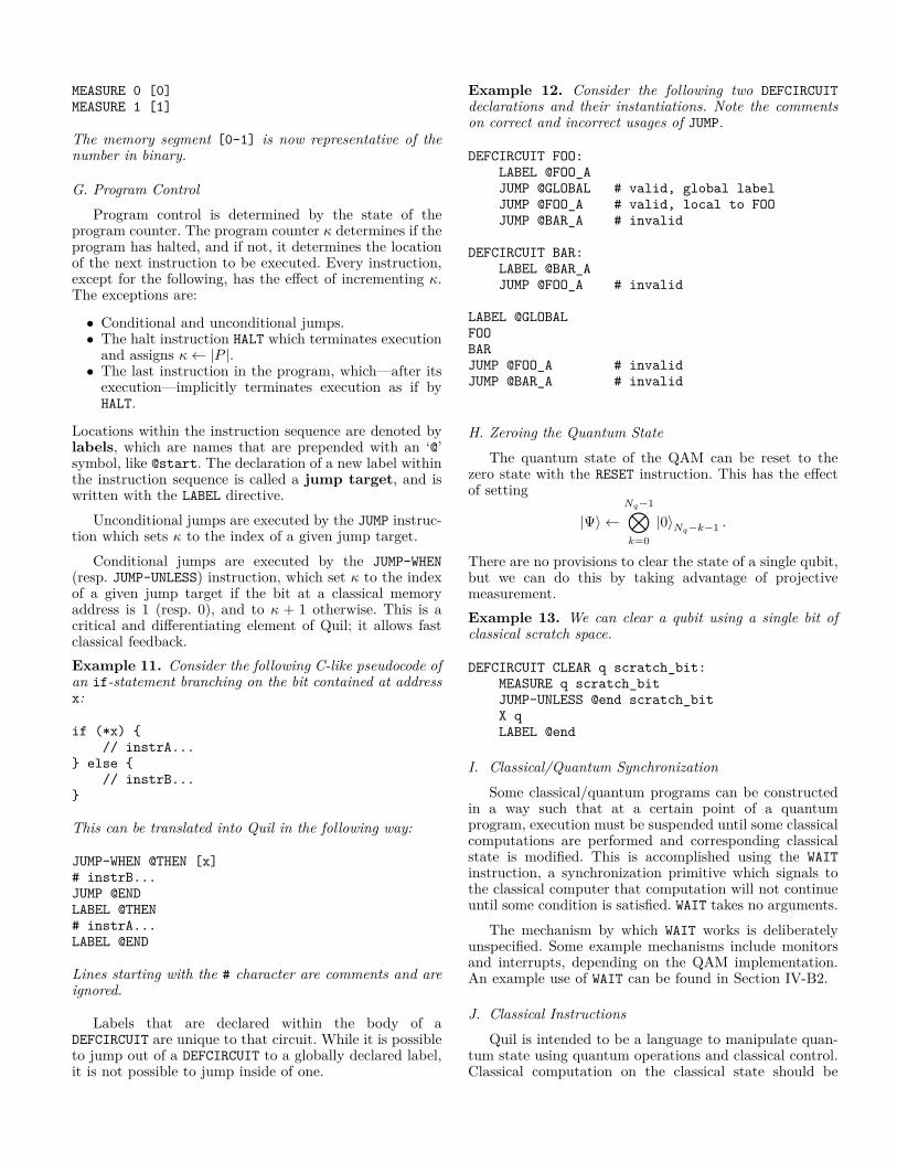
Example 12. Consider the following two DEFCIRCUITdeclarations and their instantiations. Note the commentson correct and incorrect usages of JUMP.
DEFCIRCUIT FOO:LABEL @FOO_AJUMP @GLOBAL # valid, global labelJUMP @FOO_A # valid, local to FOOJUMP @BAR_A # invalid
The quantum state of the QAM can be reset to thezero state with the RESET instruction. This has the effectof setting
|Ψ〉 ←Nq−1⊗k=0|0〉Nq−k−1 .
There are no provisions to clear the state of a single qubit,but we can do this by taking advantage of projectivemeasurement.Example 13. We can clear a qubit using a single bit ofclassical scratch space.
Some classical/quantum programs can be constructedin a way such that at a certain point of a quantumprogram, execution must be suspended until some classicalcomputations are performed and corresponding classicalstate is modified. This is accomplished using the WAITinstruction, a synchronization primitive which signals tothe classical computer that computation will not continueuntil some condition is satisfied. WAIT takes no arguments.
The mechanism by which WAIT works is deliberatelyunspecified. Some example mechanisms include monitorsand interrupts, depending on the QAM implementation.An example use of WAIT can be found in Section IV-B2.
J. Classical Instructions
Quil is intended to be a language to manipulate quan-tum state using quantum operations and classical control.Classical computation on the classical state should be
done as much as possible with a classical computer, andusing Quil’s classical/quantum synchronization to mediatethe hand-off of classical data between the classical andquantum processors. However, a few instructions for ma-nipulating the classical state are provided for convenience,with emphasis on making control flow easier.
1) Classical Unary Instructions: The classical unaryinstructions are instructions that take a single classicaladdress as an argument and modify the bit at that addressaccordingly. In each of the following, let a be the addressprovided as the sole argument. The three instructions are:
Constant False FALSE, which has the effect C[a]← 0;Constant True TRUE, which has the effect C[a]← 1; andNegation NOT, which has the effect C[a]← 1− C[a].
2) Classical Binary Instructions: The classical binaryinstructions are instructions that take two classical ad-dresses as arguments, and modify the bits at those ad-dresses accordingly. In all of the following, let a be thefirst address and b be the second address provided asarguments. The four instructions are:
Conjunction AND, which has the effect C[b]← C[a]C[b];Disjunction OR, which has the effect
C[b]← 1− (1− C[a])(1− C[b]);
Copy MOVE, which has the effect C[b]← C[a]; andExchange EXCHANGE, which has the effect of swapping the
bits at a and b: C[a]↔ C[b].Example 14. Exclusive disjunction r ← a+ b mod 2 canbe implemented with the following circuit:
DEFCIRCUIT XOR a b r:# Uses (a | b) & (˜a | ˜b)MOVE b rOR a r # r = a | bJUMP-UNLESS @end r # short-circuitMOVE b rNOT aNOT rOR a r # r = ˜a | ˜bNOT a # undo change to aLABEL @end
Note that r has to be distinct from a and b.
K. The No-Operation InstructionThe no-operation, no-op, or NOP instruction does
not affect the state of the QAM except in the way de-scribed in Section III-G, i.e., by incrementing the programcounter. This instruction may appear useless, especially ona machine with no notion of alignment or dynamic jumps.However, it has purpose when the QAM is used as thefoundation for hardware emulation. For example, considera QAM with some associated gate noise model. If onewere to use an identity gate in place of a no-op, then theidentity gate would be interpreted as noisy while the no-opwould not. Moreover, the no-op has no qubit dependencies,which would otherwise affect program analysis. RigettiComputing has used the no-op instruction as a way to
force a break in instruction parallelization, described inSection V-E.
L. File Inclusion SemanticsFile inclusion is done via the INCLUDE directive. For
example, the library of standard gates—described in Ap-pendix A—can be included with
INCLUDE "stdgates.quil"
File inclusion is not simple token substitution as it is inlanguages like the C preprocessor. Instead, the includedfile is parsed into a set of circuit definitions, gate defini-tions, and instruction code. Instruction code is substitutedverbatim, but definitions will be recorded as if they wereoriginally placed at the top of the file.
Generally, best practice is to include files containingonly contain gate or circuit definitions (in which case thefile is called a library), or only executable code, and notboth. However, this is not enforced.
M. Pragma SupportPrograms that process Quil code may want to take
advantage of extra information provided by the program-mer. This is especially true when targeting QPUs whereadditional information about the machine’s characteristicsaffect how the program will be processed. Quil supports aPRAGMA directive to include extra information in a programwhich does not otherwise affect execution semantics. Thesyntax of PRAGMA is as follows:
PRAGMA <identifier>+ <string>?
where + indicates one or more instances and ? indicateszero or one instance.Example 15. The QAM does not have any notion ofinstruction parallelism, but programs are generally par-allelized before execution on a QPU. (See Section V-E.)Programs processing Quil may wish to enforce boundariesacross which parallelization may not occur. An implemen-tation may opt to support a parallelization barrier pragma.Despite the fact that the X-gates below are commuting, animplementation may opt to treat the instructions sequen-tially.
X 0PRAGMA parallelization_barrierX 1
Note that this does not change the semantics of Quil vis-a-vis the QAM.Example 16. On modern superconducting qubit architec-tures, applications of different gates take different times.This can affect how instructions get scheduled for execution.Programs processing Quil may wish to allow the physicaltime it takes to perform a gate to be defined with a pragma,like so:
PRAGMA gate_time H "50 ns"
PRAGMA gate_time CNOT "150 ns"H 0CNOT 0 1
N. The Standard GatesQuil provides a collection of standard one-, two-,
and three-qubit gates, which are fully defined in Ap-pendix A. The standard gates can be used by includingstdgates.quil.
IV. Quil ExamplesA. Quantum Fourier Transform
In the context of the QAM’s quantum state |Ψ〉 ∈H ,the quantum Fourier transform (QFT) [23, §5.1] is aunitary operator F : H →H defined by the matrix
Fj,k := 1√2Nq
ωjk, 0 ≤ j, k < dim H = 2Nq (12)
with ω := exp(2πi/2Nq ) the complex primitive root ofunity. It can be shown that this operator acts on the basisvectors (up to permutation) via the map
Nq−1⊗k=0
k′:=Nq−k−1
|bk′〉k′ 7→1√2Nq
Nq−1⊗k=0
[|0〉k + φ(k) |1〉k] , (13)
where φ(k) =k∏j=0
exp(2πibNq−j−1/2j+1) .
Here, b is the bit string representation of the basis vectors,as in Section II-A.
The first thing to notice is that the basis elements getreversed in this factorization. This is easily fixed via aproduct of SWAP gates. In the context of classical fastFourier transforms [27], this is called bit reversal.
The second and more important thing to notice is thateach factor of the
⊗can be seen as an operation on
the qubit Qk. The factors of φ(k) indicate the operationsare two-qubit controlled-phase or CPHASE gates with Qkas the target, and each previous qubit as the control. Inthe degenerate one-qubit case, this is a Hadamard gate.Further details on this algorithm can be found in [23].
The core QFT logic can be implemented as a straight-forward recursive function QFT’. We write it as one whichtransforms qubits Qk for l ≤ k < r. The base case is theaction on a single qubit—a Hadamard. In the general case,we do a sequence of CPHASE gates targeted on the currentqubit Ql and controlled by all qubits before it, topped offby a Hadamard. In the Python-like pseudocode below, wegenerate Quil code for this algorithm. We prepend lines ofQuil code to be generated with two colons ‘::’.
def QFT’(l, r):n = r - l # num qubitsif n == 1: # base case
:: H lelse: # general case
QFT’(l + 1, r)
for i in range(1, n):q = l + n - ialpha = pi / 2 ** (n - i):: CPHASE(alpha) l q
:: H l
The bit reversal routine can be implemented straightfor-wardly as exactly bNq/2c SWAP gates.
def revbin(Nq):for i in range(Nq / 2):
:: SWAP i (Nq - i - 1)
All of this is put together in a final QFT routine.
is a classical/quantum algorithm for finding eigenvalues ofa Hamiltonian H variationally. The quantum subroutinehas two fundamental steps.
1) Prepare the quantum state |Ψ(~θ)〉, often called theansatz.
2) Measure the expectation value 〈Ψ(~θ) |H | Ψ(~θ) 〉.
The classical portion of the computation is an optimizationloop.
1) Use a classical non-linear optimizer to minimize theexpectation value by varying ansatz parameters ~θ.
2) Iterate until convergence.
We refer to given references for details on the algorithm.Practically, the quantum subroutine of VQE amounts
to preparing a state based off of a set of parameters ~θ andperforming a series of measurements in the appropriatebasis. Using the QAM, these measurements will end upin classical memory. Doing this iteratively followed by asmall amount of postprocessing, one may compute a realexpectation value for the classical optimizer to use.
This algorithm can be implemented in at least twodistinct styles which impose different requirements on aquantum computer. These two styles can serve as proto-typical examples for programming a QAM with Quil.
1) Static Implementation: One simple implementationof VQE is to generate a new Quil listing for every iterationof ~θ. Before calling out to the quantum subroutine, a newQuil program is generated for the next desired ~θ and loadedonto the quantum computer for immediate execution. Fora parameter θ = 0.00724 . . ., one such program might looklike
This technique poses no issue from the perspective ofcoherence time, but adds a time penalty to each iterationof the classical optimizer.
A static implementation of VQE was written usingRigetti Computing’s pyQuil library and the Rigetti QVM,both of which are mentioned in Sections V-B and V-Frespectively.
2) Dynamic Implementation: Perhaps the most encap-sulated implementation of VQE would be to use dynamicparameters. Without loss of generality, let’s assume asingle parameter θ. We can define a circuit which takesour single θ parameter and prepares |Ψ〉.
This program has the advantage that the quantumportion of the algorithm is completely encapsulated. It isnot necessary to dynamically reload Quil code for eachnewly varied parameter.
The main disadvantage of this approach is its im-plementation difficulty in hardware. This is because ofthe diminished potential for program analysis to occurbefore execution. The actual gates that get applied willnot be known until the runtime of the algorithm (hencethe “dynamic” name). This may limit opportunities for
Fig. 2. Outline of Forest, Rigetti Computing’s quantum program-ming toolkit, described in Section V.
optimization and poses particular issues for current quan-tum computing architectures which have limited naturalgate sets and limited high-speed dynamic tune-up of newgates or their approximations.
V. Forest: A Quantum Programming Toolkit
A. Overview
Quantum computers, and specifically QAM-conformingQPUs, are not yet widely available. Despite this, softwarecan make use of the the QAM and Quil to (a) studypractical quantum algorithmic performance in a spiritsimilar to MMIX [28], (b) prepare a suite of softwarewhich will be able to be run on QPUs, and (c) providea uniform interface to physical and virtualized QAMs.Rigetti Computing has built a toolkit called Forest foraccomplishing these tasks.
The hierarchy of software roughly falls into four layers,as in figure 2. Descending in abstraction, we have
Applications & Tools Software written to accomplishreal-world tasks (e.g., study electronic structure prob-lems), and software to assist quantum programming.
Quil The language described in this document and asso-ciated software for processing Quil. It acts as an inter-mediate representation of general quantum programs.
Compiler Software to convert arbitrary Quil to simplerQuil (or some other representation) for execution ona QPU or QVM.
Execution Units A QPU, a QVM, or a hardware emu-lator. Software written at this level will typically in-corporate noise models intrinsic to a particular QPU.
We will briefly describe each of these components of thetoolkit in the following sections.
B. Applications and ToolsQuil is an assembly-like language that is intended to
be both human readable and writable. However, moreexpressive power comes from being able to manipulateQuil programs programmatically. Rigetti Computing hasdeveloped a Python library called pyQuil [29] which allowsthe construction of Quil programs by treating them as first-class objects. Using pyQuil along with scientific librariessuch SciPy [30], Rigetti Computing has implemented non-trivial algorithms such as VQE using the abstractions ofthe QAM.
C. Quil ManipulationQuil, as a language in its own right, is amenable
to processing and computation independent of any par-ticular (real or virtual) machine for execution. RigettiComputing has written a reusable static analyzer andparser application for Quil, that allows Quil to easilybe interchanged between programs. For example, RigettiComputing’s quil-json program converts Quil into astructured JSON [31] format:
Note the two instances of “unresolved application”.These were generated because of a simple static analysisdetermining that these gates were not otherwise definedin the Quil file. (This could be ameliorated by includingstdgates.quil.)
D. CompilationIn the context of quantum computation, compilation
is the process of converting a sequence of gates into anapproximately equivalent sequence of gates executable ona quantum computer with a particular qubit topology. Thisrequires two separate kinds of processing: gate approxima-tion and routing.
Since Quil is specified as a symbolic language, it isamenable to symbolic analysis. Quil programs can be
decomposed into control flow graphs (CFGs) [32] whosenodes are basic blocks of straight-line Quil instructions, asis typical in compiler theory. Arrows between basic blocksindicate transfers of control. For example, consider thefollowing Quil program:
Roughly speaking, each segment of straight-line controlmakes up a basic block. Figure 3 depicts the control flowgraph of this program, with jump instructions elided.
*END798*Y 0MEASURE 0 [0]MEASURE 1 [1]
*EXIT-BLK-794*
*BLK-796*H 0H 1CNOT 1 0
*START795*H 0MEASURE 0 [0]
*ENTRY-BLK-793*
Fig. 3. The control flow graph of a Quil program.
Many of these basic blocks will be composed of gatesand measurements, which themselves can be symbolicallyand algebraically manipulated. Gates can go throughapproximation to reduce a general set of gates to asequence of gates native to the particular architecture, andthen routing so that these simpler gates are arrangedto act on neighboring qubits in a physical architecture.Another example of a transformation on basic blocks isparallelization, talked about in the next section.
Both approximation and routing can be formalizedas transformations between QAMs. In this first example,we show how we can formally describe a transformationbetween a QAM to another one with a smaller but com-putationally equivalent gate set.Example 17 (Compiling). Let M = (|Ψ〉 , C,GM, G
′, P, κ)be a one-qubit QAM with
GM = {H,Rx(θ),Rz(θ)}
for some fixed θ ∈ R, and let M′ be a QAM with
GM′ = {H,Rz(θ)}.
Because Rx = HRzH, we can define a compilation functionM 7→M′ specifically transforming8 ι ∈ P according to
f(ι) ={
(H,Rz(θ),H) if ι = Rx(θ),(ι) otherwise.
In this next example, we show how qubit connectivitycan be encoded in a QAM, and how one can route instruc-tions to give the illusion of a fully connected topology.Example 18 (Routing). Let M = (|Ψ〉 , C,GM, G
′, P, κ)be a three-qubit QAM with
GM = L(H) ∪ L(CNOT) ∪ L(SWAP),
where L was defined in Example 4. Consider a three-qubitQPU with the qubits arranged in a line
Q0—Q1—Q2
so that two-qubit gates can only be applied on adjacentqubits. Then this QPU can be modeled by another three-qubit QAM M′ with the lifted gates
GM′ ={ H0,H1,H2,
CNOT01,CNOT10,CNOT12,CNOT21,SWAP01,SWAP12
}.
Because of the qubit topology, there are no gates that acton B2 ⊗B0. However, we can reason about transformingbetween M and M′ in either direction. We can transformfrom M to M′ by way of a transformation f similar to thatin the last example, namely
f(ι) =
(SWAP01,SWAP12,SWAP01) if ι = SWAP02,(SWAP01,CNOT12,SWAP01) if ι = CNOT02,(SWAP01,CNOT21,SWAP01) if ι = CNOT20,(ι) otherwise.
Similarly, we can transform from M′ to M by adding threeadditional gates to GM′ , namely those implied by f .
Many other classes of useful transformations on QAMsexist, such as G-preserving algebraic simplifications of P ,an analog of peephole optimization in compiler theory [33].
E. Instruction Parallelism
Instruction parallelism, the ability to apply com-muting operations to a quantum state in parallel, is oneof the many benefits of quantum computation. Quil codeas written is linear and serial, but can be interpretedas an instruction-parallel program. In particular, manysubsequences of Quil instructions may be executed inparallel. Such sequences include:
• Commuting gate applications and measurements, and• Measurements with non-overlapping memory ad-
dresses.8In the parlance of functional programming, f is applied to P via
a concatmap operation.
In general, parallelization cannot occur over jumps, resets,waits, and measurements and dynamic gate applicationswith overlapping address ranges. We suggest that NOP isused as a way to force a parallelization break.
If a control flow graph is constructed as in Section V-D,then parallelization can be done over each basic block. Aparallelized basic block is called a parallelization sched-ule. See Figure 4 for an example of quantum parallelizationwithin a CFG.
*END804*{ Y 0 MEASURE 1 [1]}{ MEASURE 0 [0]}
*EXIT-BLK-800*
*BLK-802*{ H 0 H 1}{ CNOT 1 0}
*START801*{ H 0}{ MEASURE 0 [0]}
*ENTRY-BLK-799*
Fig. 4. The parallelized version of Figure 3. Instruction sequenceswhich can be executed in parallel are surrounded in curly braces ‘{}’.
F. Rigetti Quantum Virtual Machine
Rigetti Computing has implemented a QVM in ANSICommon Lisp [34] called the Rigetti QVM. It is a high-performance9, programmable simulator for the QAM andemulator for noisy quantum computers. The Rigetti QVMexposes two interfaces for executing quantum programs:execution of Quil files directly with POSIX-style sharedmemory (“local execution”), and execution of Quil fromHTTP server requests (“remote execution”).
Local execution is useful for high-speed testing ofsmall-to-medium sized instances of classical/quantum al-gorithms. It also provides convenient ways of debuggingquantum programs, such as allowing direct inspection ofthe quantum state at any point in the execution process, aswell as limited quantum hardware emulation with tunablenoise models.
Remote execution is used for distributed, cloud accessto QVM instances. HTTP libraries exist in nearly allmodern programming languages, and allow programs in
9The Rigetti QVM has optimized vectorized and parallelized nu-merics, and has no theoretical limit for the number of qubits it cansimulate. It has been demonstrated to simulate 36 qubits.
these languages to make connections. Rigetti Computinghas built in to pyQuil the ability to send the first-classQuil program objects to a local or secured remote RigettiQVM instance using the Forest API.
VI. ConclusionWe have introduced a practical abstract machine for
reasoning about and executing quantum programs. Fur-thermore, we have described a notation for such programson this machine, which is amenable to analysis, compila-tion, and execution. Finally, we have described a pragmatictoolkit for quantum program construction and executionbuilt atop these ideas.
VII. AcknowledgementsThe authors would like to thank their colleagues at
Rigetti Computing for their support, especially Nick Ru-bin. We are also grateful to Erik Davis, Jarrod McClean,Bill Millar, and Eric Peterson for their helpful discussionsand valuable suggestions provided throughout the devel-opment of this work.
AppendixA. The Standard Gate Set
The following static and parametric gates are definedin stdgates.quil. Many of these gates are standard gatesused in theoretical quantum computation [23], and someof them find their origin in the theory of superconductingqubits [35].
There exists much literature on abstract models, syn-taxes, and semantics of quantum computing. Most ofthem are in the form of quantum programming languages(QPLs) and simulators, which achieve various levels of ex-pressiveness. Languages roughly fall into three categories:
In addition, work has been done on designing larger toolchains for quantum programming [18, 19, 36].
In the following subsections, we provide a non-exhaustive account of some previous work within the abovecategories, and describe how they relate to the design ofour quantum ISA.
1) Embedded Domain-Specific Languages: An embed-ded domain-specific language (EDSL) is a languageto express concepts and problems from within anotherprogramming language. Within the context of quantumprogramming, two prominent examples are Quipper [16],which is embedded in Haskell [37], and LIQUi|〉 [15],which is embedded in F# [38]. Representation of quantumprograms (and, in particular, the subclass of quantumprograms called quantum circuits) is expressed with datastructures in the host language. Feedback of classicalinformation is achieved through an interface with the hostlanguage.
Quantum programs written in an EDSL are not directlyexecutable on a quantum computer, due to the require-ment of being present in the host language’s runtime.However, since quantum programs are represented as first-class objects, these objects are amenable to processing andcompilation to a quantum computer’s natively executableinstruction set. Quil is one such target for compilation.
2) High-Level QPLs: High-level QPLs are the quantumanalog of languages like C [39] in the imperative case orML [40] in the functional case. They provide a plethora ofclassical and quantum data types, as well as control flowconstructs. In the case of functional quantum languages,the lambda calculus for quantum computation with classi-cal control by Selinger and Valiron can act as a theoreticalbasis for their semantics of such a language10 [42].
10This is similar to how the classical untyped lambda calculusformed the basis for LISP in 1958 [41].
One prominent example of a high-level QPL is Bern-hard Omer’s QCL [43]. It is a C-like language with clas-sical control and quantum data. Among the many thatexist, two important—and indeed somewhat dual—datatypes are int and qureg. The following example showsa Hadamard initialization on eight qubits, and measuringthe first four of those qubits into an integer variable.
// Allocate classical and quantum dataqureg q[8];int m;// Hadamard initializeH(q);// Measure four qubits into mmeasure q[0..3], m;// Print m, which will be anywhere from 0 to 15.print m;
Omer defines the semantics of this language in detail inhis PhD thesis, and presents an implementation of a QCLinterpreter written in C++ [44]. However, a compilation orexecution strategy on quantum hardware is not presented.Similar to EDSLs, QPLs such as QCL can be compiledinto a lower-level quantum instruction set such as Quil.
3) Low-Level Quantum Intermediate Representations:In the context of compiler theory, an intermediate rep-resentation (IR) is some representation of a languagewhich is amenable to further processing. IR can be higherlevel (as with abstract syntax trees), or lower level (aswith linear bytecodes). Low-level IRs often act as compila-tion targets for classical programming languages, and areused for analysis and program optimization. For example,LLVM IR [45] is used as an intermediate compilation targetfor the Clang C compiler [46].
The most well-known example of a low-level quantumIR is QASM [47]. This was originally a language to describethe quantum circuits for LATEX output in [23], and hence,not an IR in that form. However, the syntax was adaptedfor executable use in [48]. QASM, however, does not haveany notion of classical control within the language, actingsolely as a quantum circuit description language.
Quil is considered a low-level quantum IR with classicalcontrol.
References
[1] P. J. J. O’Malley, R. Babbush, I. D. Kivlichan,J. Romero, J. R. McClean, R. Barends, J. Kelly,P. Roushan, A. Tranter, N. Ding, B. Campbell,Y. Chen, Z. Chen, B. Chiaro, A. Dunsworth,A. G. Fowler, E. Jeffrey, E. Lucero, A. Megrant,J. Y. Mutus, M. Neeley, C. Neill, C. Quintana,D. Sank, A. Vainsencher, J. Wenner, T. C. White,P. V. Coveney, P. J. Love, H. Neven, A. Aspuru-Guzik, and J. M. Martinis, “Scalable quantumsimulation of molecular energies,” Phys. Rev. X,vol. 6, p. 031007, Jul 2016. [Online]. Available:http://link.aps.org/doi/10.1103/PhysRevX.6.031007
[2] M. R. Geller, J. M. Martinis, A. T. Sornborger, P. C.Stancil, E. J. Pritchett, H. You, and A. Galiautdi-
nov, “Universal quantum simulation with prethresh-old superconducting qubits: Single-excitation sub-space method,” Physical Review A, vol. 91, no. 6, p.062309, 2015.
[3] R. Barends, A. Shabani, L. Lamata, J. Kelly, A. Mez-zacapo, U. Las Heras, R. Babbush, A. Fowler,B. Campbell, Y. Chen et al., “Digitized adiabaticquantum computing with a superconducting circuit,”Nature, vol. 534, no. 7606, pp. 222–226, 2016.
[4] D. Riste, M. P. da Silva, C. A. Ryan, A. W. Cross,J. A. Smolin, J. M. Gambetta, J. M. Chow, and B. R.Johnson, “Demonstration of quantum advantage inmachine learning,” arXiv preprint arXiv:1512.06069,2015.
[5] J. M. Chow, S. J. Srinivasan, E. Magesan, A. Corcoles,D. W. Abraham, J. M. Gambetta, and M. Steffen,“Characterizing a four-qubit planar lattice for arbi-trary error detection,” in SPIE Sensing Technology+Applications. International Society for Optics andPhotonics, 2015, pp. 95 001G–95 001G.
[6] J. Kelly, R. Barends, A. Fowler, A. Megrant, E. Jef-frey, T. White, D. Sank, J. Mutus, B. Campbell,Y. Chen et al., “State preservation by repetitive er-ror detection in a superconducting quantum circuit,”Nature, vol. 519, no. 7541, pp. 66–69, 2015.
[7] D. Riste, S. Poletto, M.-Z. Huang, A. Bruno,V. Vesterinen, O.-P. Saira, and L. DiCarlo, “Detect-ing bit-flip errors in a logical qubit using stabilizermeasurements,” Nature communications, vol. 6, 2015.
[8] A. Peruzzo, J. McClean, P. Shadbolt, M.-H. Yung,X.-Q. Zhou, P. J. Love, A. Aspuru-Guzik, and J. L.O’Brien, “A variational eigenvalue solver on a pho-tonic quantum processor,” Nature communications,vol. 5, 2014.
[9] D. Wecker, M. B. Hastings, and M. Troyer, “Progresstowards practical quantum variational algorithms,”Physical Review A, vol. 92, no. 4, p. 042303, 2015.
[10] J. R. McClean, J. Romero, R. Babbush, andA. Aspuru-Guzik, “The theory of variational hy-brid quantum-classical algorithms,” New Journal ofPhysics, vol. 18, no. 2, p. 023023, 2016.
[11] B. Bauer, D. Wecker, A. J. Millis, M. B. Hast-ings, and M. Troyer, “Hybrid quantum-classicalapproach to correlated materials,” arXiv preprintarXiv:1510.03859, 2015.
[12] E. Farhi, J. Goldstone, and S. Gutmann, “A quantumapproximate optimization algorithm,” arXiv preprintarXiv:1411.4028, 2014.
[13] M. Reiher, N. Wiebe, K. M. Svore, D. Wecker, andM. Troyer, “Elucidating reaction mechanismson quantum computers,” arXiv preprintarXiv:1605.03590, 2016.
[14] D. Deutsch, “Quantum Theory, the Church–TuringPrinciple and the Universal Quantum Computer,”Proceedings of the Royal Society of London A: Mathe-matical, Physical and Engineering Sciences, vol. 400,no. 1818, pp. 97–117, 1985.
[15] D. Wecker and K. M. Svore, “LIQUi|〉: A SoftwareDesign Architecture and Domain-Specific Languagefor Quantum Computing,” 2014. [Online]. Available:arXiv:1402.4467v1
[16] A. S. Green, P. L. Lumsdaine, N. J. Ross, P. Selinger,
and B. Valiron, “Quipper: A scalable quantumprogramming language,” SIGPLAN Not., vol. 48,no. 6, pp. 333–342, Jun. 2013. [Online]. Available:http://doi.acm.org/10.1145/2499370.2462177
[17] T. Haner, D. S. Steiger, K. Svore, and M. Troyer,“A software methodology for compiling quantum pro-grams,” arXiv preprint arXiv:1604.01401, 2016.
[18] K. M. Svore, A. V. Aho, A. W. Cross, I. Chuang,and I. L. Markov, “A layered software architecture forquantum computing design tools,” IEEE Computer,vol. 39, no. 1, pp. 74–83, 2006.
[19] A. JavadiAbhari, S. Patil, D. Kudrow, J. Heckey,A. Lvov, F. T. Chong, and M. Martonosi, “Scaffcc:Scalable compilation and analysis of quantum pro-grams,” Parallel Computing, vol. 45, pp. 2–17, 2015.
[20] T. Haner, D. S. Steiger, M. Smelyanskiy, andM. Troyer, “High performance emulation of quantumcircuits,” arXiv preprint arXiv:1604.06460, 2016.
[21] M. Smelyanskiy, N. P. Sawaya, and A. Aspuru-Guzik, “qhipster: the quantum high performancesoftware testing environment,” arXiv preprintarXiv:1601.07195, 2016.
[22] A. Barenco, C. H. Bennett, R. Cleve, D. P. DiVin-cenzo, N. Margolus, P. Shor, T. Sleator, J. A. Smolin,and H. Weinfurter, “Elementary gates for quantumcomputation,” Physical review A, vol. 52, no. 5, p.3457, 1995.
[23] M. A. Nielsen and I. L. Chuang, Quantum computa-tion and quantum information. Cambridge UniversityPress, 2010.
[24] D. Deutsch, A. Barenco, and A. Ekert, “Universalityin quantum computation,” in Proceedings of the RoyalSociety of London A: Mathematical, Physical andEngineering Sciences, vol. 449, no. 1937. The RoyalSociety, 1995, pp. 669–677.
[25] S. Aaronson, Quantum computing since Democritus.Cambridge University Press, 2013.
[26] IEEE standard for binary floating-point arithmetic,New York, 1985, note: Standard 754–1985.
[27] J. W. Cooley and J. W. Tukey, “An algorithm forthe machine calculation of complex fourier series,”Mathematics of computation, vol. 19, no. 90, pp. 297–301, 1965.
[28] D. E. Knuth, The Art of Computer Programming,Volume 1, Fascicle 1: MMIX – A RISC Computer forthe New Millennium (Art of Computer Programming).Addison-Wesley Professional, 2005.
[30] E. Jones, T. Oliphant, P. Peterson et al., “SciPy:Open source scientific tools for Python,” 2001–2016, accessed: 2016-06-21. [Online]. Available: http://www.scipy.org/
[31] The JSON Data Interchange For-mat, 1st ed., October 2013. [On-line]. Available: http://www.ecma-international.org/publications/files/ECMA-ST/ECMA-404.pdf
[32] F. E. Allen, “Control flow analysis,” SIGPLAN Not.,vol. 5, no. 7, pp. 1–19, Jul. 1970. [Online]. Available:http://doi.acm.org/10.1145/390013.808479
[34] American National Standards Institute and Informa-tion Technology Industry Council, American NationalStandard for Information Technology: programminglanguage — Common LISP, American National Stan-dards Institute, 1430 Broadway, New York, NY 10018,USA, 1996, approved December 8, 1994.
[35] J. M. Chow, “Quantum information processing withsuperconducting qubits,” Ph.D. dissertation, YaleUniversity, 2010.
[36] A. J. Abhari, A. Faruque, M. J. Dousti, L. Svec,O. Catu, A. Chakrabati, C.-F. Chiang, S. Vanderwilt,J. Black, and F. Chong, “Scaffold: Quantum program-ming language,” DTIC Document, Tech. Rep., 2012.
[37] S. Marlow, “Haskell 2010 Language Report,” https://www.haskell.org/definition/haskell2010.pdf, 2010, ac-cessed: 2016-06-21.
[38] D. Syme et al., “The F# 4.0 Language Specifi-cation,” http://fsharp.org/specs/language-spec/4.0/FSharpSpec-4.0-latest.pdf, 2016, accessed: 2016-06-21.
[39] B. W. Kernighan, The C Programming Language,2nd ed., D. M. Ritchie, Ed. Prentice Hall ProfessionalTechnical Reference, 1988.
[40] R. Milner, M. Tofte, and D. Macqueen, The Definitionof Standard ML. Cambridge, MA, USA: MIT Press,1997.
[41] J. McCarthy, “Recursive functions of symbolic ex-pressions and their computation by machine, part i,”Communications of the ACM, vol. 3, no. 4, pp. 184–195, 1960.
[42] P. Selinger and B. Valiron, “A lambda calculus forquantum computation with classical control,” Math-ematical Structures in Computer Science, vol. 16,no. 03, pp. 527–552, 2006.
[43] B. Omer, “Structured quantum programming,” Ph.D.dissertation, Technical University of Vienna, 2003.[Online]. Available: http://tph.tuwien.ac.at/∼oemer/doc/structquprog.pdf
[44] ——, “QCL - A Programming Language for Quan-tum Computers,” http://tph.tuwien.ac.at/∼oemer/qcl.html, 2014, accessed: 2016-06-30.
[45] C. Lattner and V. Adve, “LLVM: A CompilationFramework for Lifelong Program Analysis & Trans-formation,” in Proceedings of the 2004 InternationalSymposium on Code Generation and Optimization(CGO’04), Palo Alto, California, Mar 2004.
[46] Clang developers, “clang: a C language family fron-tend for LLVM,” http://clang.llvm.org/, accessed:2016-06-30.
[47] MIT Quanta Group, “Quantum circuit viewer:qasm2circ,” http://www.media.mit.edu/quanta/qasm2circ/, accessed: 2016-06-30.