HAL Id: hal-00908965 https://hal.archives-ouvertes.fr/hal-00908965v1 Submitted on 25 Nov 2013 (v1), last revised 15 Jun 2016 (v2) HAL is a multi-disciplinary open access archive for the deposit and dissemination of sci- entific research documents, whether they are pub- lished or not. The documents may come from teaching and research institutions in France or abroad, or from public or private research centers. L’archive ouverte pluridisciplinaire HAL, est destinée au dépôt et à la diffusion de documents scientifiques de niveau recherche, publiés ou non, émanant des établissements d’enseignement et de recherche français ou étrangers, des laboratoires publics ou privés. A pressurized model for compressible pipe flow. Mehmet Ersoy To cite this version: Mehmet Ersoy. A pressurized model for compressible pipe flow.. 2013. <hal-00908965v1>
Transcript
HAL Id: hal-00908965https://hal.archives-ouvertes.fr/hal-00908965v1
Submitted on 25 Nov 2013 (v1), last revised 15 Jun 2016 (v2)
HAL is a multi-disciplinary open accessarchive for the deposit and dissemination of sci-entific research documents, whether they are pub-lished or not. The documents may come fromteaching and research institutions in France orabroad, or from public or private research centers.
L’archive ouverte pluridisciplinaire HAL, estdestinée au dépôt et à la diffusion de documentsscientifiques de niveau recherche, publiés ou non,émanant des établissements d’enseignement et derecherche français ou étrangers, des laboratoirespublics ou privés.
A pressurized model for compressible pipe flow.Mehmet Ersoy
To cite this version:
Mehmet Ersoy. A pressurized model for compressible pipe flow.. 2013. <hal-00908965v1>
1Universite de Toulon, IMATH, EA 2134, 83957 La Garde, France.
Abstract
We present the full derivation of a compressible model in a thin closed water pipe including friction,changes of section and slope variation. Starting from the compressible 3D Navier-Stokes equation under”thin layer” assumptions with well-suited boundary conditions, we justify the 1D reduced model calledpressurized model (also named the P-model). It was introduced in the general framework of unsteadymixed flows in closed water pipes. This model describes the evolution of a compressible flow close to gasdynamics equations in a nozzle. We also propose a class of averaged low Oser compressible models of ageneral barotropic law p(ρ) = ρ
Simulation of pressurized flows (i.e. the pipe is full) as well as free surface (i.e. only a part of the pipe isfilled) in closed water pipe plays an important role in many engineering applications such as storm sewers,waste or supply pipes in hydroelectric installations . . . . The transition phenomenon between the two typesof flows occurs in many situations and it can be induced by sudden change in the boundary conditions asfailure pumping. During this process, in particular for pressurized flows, the pressure can reach severe valuesand may cause irreversible damage. Accurate mathematical and numerical models are required to predictand to avoid such a situation.
From a numerical viewpoint, the use of the full 3D Navier-Stokes equations lead to time-consumingsimulations. Introducing reduced models preserving some of the main physical features is one of the mostchallenging issues that we address with the obvious consequence to decrease the computational time. Dur-ing these last years, a great amount of works was devoted to the modeling and the simulation of such aphenomenon (see for instance [18, 25, 24, 10, 9, 16], [8, 3, 2, 11, 4, 5] and the reference therein).
The classical shallow water equations, commonly used to describe free surface flows in open channels,are also used in the study of pressurized flows with the artifice of the Preissman (see for example [9, 28])assuming a narrow slot to exist in the upper part of the pipe. The width of the slot is calibrated toprovide the correct sonic speed. Nevertheless, as pointed out by several authors (see [25] for instance),the pressurizing phenomenon is a dynamic shock requiring a full dynamic treatment even if the inflowsand other boundary conditions change slowly. Moreover, the Preissman slot artefact is unable to take intoaccount the depressurisation phenomenon (i.e. sub-atmospheric flows) which occurs during a water hammer.On the other hand the commonly used model to describe pressurized flows in closed water pipes are theAllievi equations which are derived by neglecting some acceleration terms. As a consequence, the resultingfirst order system is not written under a conservative form and thus it is not well adapted to a natural
coupling with a shallow water model which describes the evolution of free surface flows in closed waterpipes. Thus, the pressurized model was formally introduced by the author in [11, 5] as an extension of thework by Bourdarias and Gerbi [8]. The obtained 1D equations for pressurized flows was derived from the3D isentropic compressible Euler equations to take into account sub-atmospheric flows with a formulationclosed to the Saint-Venant equations for free surface flows. As a consequence, the free surface model and thepressurized model was coupled to construct a ”unified” model for unsteady mixed water flows. The formalderivation of this model, called PFS-model (see [11, 5]), as well as a finite volume discretization have beenpreviously proposed by Bourdarias and Gerbi [8]. This works was extended by the author [5] in the case ofnon uniform section and a new VFRoe solver [3] as well as a new kinetic solver [2, 4] have been proposed.
Although, all of these models was formally derived, numerical experiment versus laboratory experimentwas presented [3, 2, 4]) and the proposed schemes for the P-model, as well as for the PFS-model, produceresults that are in a very good agreement. Under the hypothesis
u ≈ u and ρu ≈ ρ u
the P-model is an accurate approximation of the Euler equations in a ”thin-layer” framework. The so-calledpressurized model is:
∂tA+ ∂xQ = 0,
∂tQ+ ∂x
(
Q2
A+ c2(A− S)
)
= −gA sin θ + c2(
A
S− 1
)
dS
dx
(1)
where ρ is the mean density of the water, A = ρS is the equivalent wet area, u is the mean water velocity,Q = Au is the equivalent discharge, S is the section of the pipe, c is the sonic speed and sin θ is the ”slopevariation”. To take into account the friction, a quadratic term −ρgCfu|u| was added to the system (1). Thefriction factor Cf is defined by
Cf =1
K2sRh(S(x))4/3
,
where Ks is the Strickler coefficient of roughness depending on the material, Rh(S) = S/Pm is the hydraulicradius and Pm is the perimeter of the pipe’s section.
We propose here to justify the pressurized model as an approximation at order O(ε) of the full 3Dcompressible Navier-Stokes system where ε is the aspect ratio assumed to be small
ε =D
L≪ 1 ,
as recently done by Ersoy [12] for the 3D-1D reduced free surface model in open channel and closed waterpipe. In particular, we show that the ”motion by slices” assumption,
u ≈ u and ρu ≈ ρ u
used to formally derive the pressurized model, are exact at first order and
u = u+O(ε), ρu = ρ u+O(ε) .
These results are obtained with well suited boundary conditions including friction and the pressure law ischosen as a linear one p(ρ) = c2(ρ−ρ0). It allows to take into account sub-atmospheric and sup-atmosphericflows where ρ0 stands for the density of the water at atmospheric pressure.
Moreover, assuming that the Oser number, the ratio between the Mach number and the Froude number,is small, we derive a class of averaged compressible models in a closed water pipe with a general pressurelaw p(ρ) = ργ for γ > 1. In particular, we show that at first order
ργ = ργ
which is wrong in general if the Oser number is not small enough.
2
The paper is organized as follows. In Section 2, we recall the compressible Navier-Stokes equations withsuitable boundary conditions including friction and we fix the notations. In Section 3, we first deduce theso-called motion by slices and other assumptions required to derive the pressurized model under thin-layerassumptions from the hydrostatic approximation of the compressible Navier-Stokes equations. Then, theseequations are integrated following the section orthogonal to the main flow direction and the 1D pressurizedmodel is obtained. Finally, we end with Section 4 where we discuss about a class of averaged low Osercompressible models in a thin-layer domain.
2 The compressible Navier-Stokes equations and its closure
In this section, we fix the notations of the geometrical quantities involved to describe the thin closed do-main representing a pipe. Then, we recall the compressible Navier-Stokes system written in the Cartesiancoordinates with a gravity. We define the wall-law boundary conditions to include a general friction lawcompleted with a no penetration condition. For the sake of simplicity, we do not deal with the deformationof the domain induced by the change of pressure. For the case of deformation of the pipe due to the changeof pressure, we refer to the work by Bourdarias and Gerbi [8] where a Hooke’s law is used. We will consideronly an infinitely rigid pipe with circular sections.
2.1 Notations and settings
Let us consider a compressible fluid confined in a three dimensional domain P , a pipe of length L orientedfollowing the i vector,
P :=
(x, y, z) ∈ R3; x ∈ [0, L], (y, z) ∈ Ω(x)
where the section Ω(x), x ∈ [0, L], is
Ω(x) = (y, z) ∈ R2; y ∈ [α(x, z), β(x, z)], z ∈ [−R(x), R(x)]
as displayed on figure 1(a).The main flow direction is supposed to be in the i direction. Thus the section Ω(x), x ∈ [0, L], is assumed
to be orthogonal to the main flow direction.Here R(x) stands for the radius of the pipe section S(x) = πR2(x), α(x, z) (resp. β(x, z)) is the left
(resp. the right) boundary point at elevation −R(x) 6 z 6 R(x).In the Ω-plane, we define the coordinate of a point m ∈ ∂Ω(x), x ∈ [0, L], by (y, ϕ(x, y)) where ϕ(x, y) =
√
R(x)2 − y2 for y > 0 and ϕ(x, y) = −√
R(x)2 − y2 for y < 0. The point m stands for the vector ωm
where w(x, 0, b(x)) defines the main slope elevation of the pipe with b′(x) = sin θ(x). Then, we note n =m
|m|the outward unit vector at the point m ∈ ∂Ω(x), x ∈ [0, L] as represented on figure 1(b).
(a) Configuration (b) Ω-plane
Figure 1: Geometric characteristics of the pipe
3
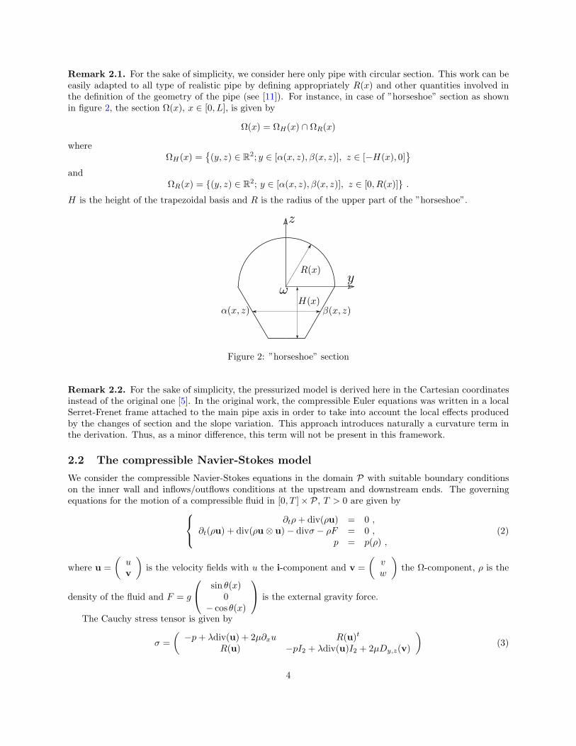
Remark 2.1. For the sake of simplicity, we consider here only pipe with circular section. This work can beeasily adapted to all type of realistic pipe by defining appropriately R(x) and other quantities involved inthe definition of the geometry of the pipe (see [11]). For instance, in case of ”horseshoe” section as shownin figure 2, the section Ω(x), x ∈ [0, L], is given by
Ω(x) = ΩH(x) ∩ ΩR(x)
whereΩH(x) =
(y, z) ∈ R2; y ∈ [α(x, z), β(x, z)], z ∈ [−H(x), 0]
andΩR(x) = (y, z) ∈ R2; y ∈ [α(x, z), β(x, z)], z ∈ [0, R(x)] .
H is the height of the trapezoidal basis and R is the radius of the upper part of the ”horseshoe”.
Figure 2: ”horseshoe” section
Remark 2.2. For the sake of simplicity, the pressurized model is derived here in the Cartesian coordinatesinstead of the original one [5]. In the original work, the compressible Euler equations was written in a localSerret-Frenet frame attached to the main pipe axis in order to take into account the local effects producedby the changes of section and the slope variation. This approach introduces naturally a curvature term inthe derivation. Thus, as a minor difference, this term will not be present in this framework.
2.2 The compressible Navier-Stokes model
We consider the compressible Navier-Stokes equations in the domain P with suitable boundary conditionson the inner wall and inflows/outflows conditions at the upstream and downstream ends. The governingequations for the motion of a compressible fluid in [0, T ]× P , T > 0 are given by
is the velocity fields with u the i-component and v =
(
vw
)
the Ω-component, ρ is the
density of the fluid and F = g
sin θ(x)0
− cos θ(x)
is the external gravity force.
The Cauchy stress tensor is given by
σ =
(
−p+ λdiv(u) + 2µ∂xu R(u)t
R(u) −pI2 + λdiv(u)I2 + 2µDy,z(v)
)
(3)
4
where I2 is the identity matrix, µ is the dynamical viscosity and R(u) is defined by R(u) = µ (∇y,zu+ ∂xv).
Here, ∇y,zu =
(
∂yu∂zu
)
is the gradient of u with respect to (y, z). Noting ·t the transpose of ·, we define
the strain tensor Dy,z(v) with respect to the variable (y, z):
2Dy,z(u) = ∇y,zv+∇ty,zv .
The last term λdiv(u) is the classical normal stress tensor which plays an important role when the fluid israpidly compressed or expanded, such as in shock waves. The quantity λ is the volume viscosity, often calledsecond viscosity, is usually assumed to be of the same order of magnitude as the dynamical viscosity µ (see[20]).
Remark 2.3. In the literature, there exists several approach to define the stress tensor in order to set aprivileged flow direction.For incompressible fluids, one has for instance,
• Gerbeau and Perthame [17] use an isotropic stress tensor with constant viscosity to derive the Saint-Venant equations from the 2D incompressible Navier-Stokes equations,
• Marche [21] or Ferrari and Saleri [15], in a similar way, derive a two dimensional shallow water equationsfrom the 3D incompressible Navier-Stokes equations.
In the case of compressible fluids, Ersoy et al [14, 13] (based on the work by Kochin [19]) use the followinganisotropic total stress tensor:
σ = −pI3 + 2Σ.D(u) + λdiv(u) I3
to set a privileged horizontal flow direction in the context of atmosphere modeling. The term Σ.D(u) isdefined as:
(
2µDx(u) µ2R(u)t
µ3R(u) 2µ3∂yv
)
where I3 is the identity matrix and Σ = Σ(t, x, y) is the anisotropic viscous tensor:
In their case, they obtain a viscous hydrostatic approximation called Compressible Primitive Equations.In no instance, up to our knowledge, there are now works (except the free surface model by Ersoy [12])
which justify a 1D model from a 3D model in a thin-layer framework.
Finally, the pressure law is given by the following equation of state:
p(ρ) = c2ρ (4)
where c is the sonic speed.
Remark 2.4. In practice, c =1√β0ρ0
≈ 1400m2/s where β0 ≈ 5.0 10−10m2/N is the inverse of the bulk
modulus of compression of the water and ρ0 is the volumetric mass of water.
Remark 2.5. In practical applications, we set
p(ρ) = pa + c2(ρ− ρ0)
which has the advantage to show clearly overpressure state and depression state. Indeed, the overpressurestate corresponds to ρ > ρ0 while ρ < ρ0 represents a depression state. The case ρ = ρ0 is a critic one and abifurcation point in the context of unsteady mixed flows (see [11, 5] for further details).
5
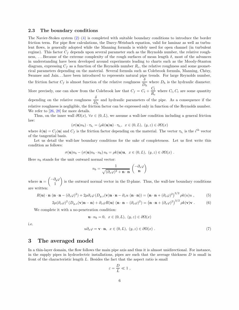
2.3 The boundary conditions
The Navier-Stokes system (2)–(4) is completed with suitable boundary conditions to introduce the borderfriction term. For pipe flow calculations, the Darcy-Weisbach equation, valid for laminar as well as turbu-lent flows, is generally adopted while the Manning formula is widely used for open channel (in turbulentregime). This factor Cf depends upon several parameter such as the Reynolds number, the relative rough-ness, . . . Because of the extreme complexity of the rough surfaces of mean length δ, most of the advancesin understanding have been developed around experiments leading to charts such as the Moody-Stantondiagram, expressing Cf as a function of the Reynolds number Re, the relative roughness and some geomet-rical parameters depending on the material. Several formula such as Colebrook formula, Manning, Chezy,Swamee and Jain. . . have been introduced to represents natural pipe trends. For large Reynolds number,
the friction factor Cf is almost function of the relative roughnessδ
Dhwhere Dh is the hydraulic diameter.
More precisely, one can show from the Colebrook law that Cf = Ct +Cl
Rewhere Cl, Ct are some quantity
depending on the relative roughnessδ
Dhand hydraulic parameters of the pipe. As a consequence if the
relative roughness is negligible, the friction factor can be expressed only in function of the Reynolds number.We refer to [26, 28] for more details.
Thus, on the inner wall ∂Ω(x), ∀x ∈ (0, L), we assume a wall-law condition including a general frictionlaw:
i.e.u∂xϕ = v · n, x ∈ (0, L), (y, z) ∈ ∂Ω(x) . (7)
3 The averaged model
In a thin-layer domain, the flow follows the main pipe axis and thus it is almost unidirectional. For instance,in the supply pipes in hydroelectric installations, pipes are such that the average thickness D is small infront of the characteristic length L. Besides the fact that the aspect ratio is small
ε =D
L≪ 1 ,
6
we should assume that the characteristic speed in the Ω-plane V = (V,W ) is small compared to the horizontalone U :
W
U≈ V
U≪ 1
in order to get a unidirectional flow. These physical considerations define the so-called ”thin-layer” assump-tions.
3.1 The adimensionnalised Navier-Stokes equations
Thus, in the sequel we adimensionnalise the Navier-Stokes system using the ”thin-layer” assumptions byintroducing a ”small” parameter
ε =D
L=W
U=V
U≪ 1.
We then introduce a characteristic time T such that T =L
Uand we note ρ0 a characteristic density of
the water. The dimensionless quantities of time t, coordinate (x, y, z), velocity field (u, v, w) and of density
ρ, noted temporarily by a ·, are defined by x =x
X. Thus, one has
t =t
T, (x, y, z) =
( x
L,y
D,z
D
)
, (u, v, w) =( u
U,v
W,w
W
)
, ρ =ρ
ρ0.
We finally define the modified friction factor Cf/U that we write Cf .We introduce the non-dimensional numbers:
Fr Froude number following the Ω-plane : Fr =U√gD
,
FL Froude number following the i-direction : FL =U√gL
,
Rµ Reynolds numbers with respect to µ : Rµ =ρ0UL
µ,
Rλ Reynolds numbers with respect to λ : Rλ =ρ0UL
λ,
Ma Mach number : Ma =U
c,
C Oser number : C =Ma
Fr=
√gD
c
where the dimensionless number C is often referred as the Oser number. It determines whether the gravityshould have an influence or not in the model. Let us note that the Oser number may have influence forlaw temperature model. In such cases, the gravity effect can be considerable (we refer to Section 4.1 fornumerical illustration).
Remark 3.1. In view of Remark 2.4, in practice, the Oser number is C ≈ 1
1000. Thus, this parameter
indicates that the fluid is slightly influenced by the effects of the gravity in the present modeling problem.
Dropping the ·, the non-dimensional compressible Navier-Stokes system becomes:
∂tρ+ ∂x(ρu) + divy,z(ρv) = 0 ,
∂t(ρu) + ∂x(ρu2) + divy,z(ρuv) + ∂x
ρ
M2a
= Gρu ,
ε2 (∂t(ρv) + ∂x(ρuv) + divy,z(ρv⊗ v)) +∇y,zρ
M2a
= Gρv ,
(8)
7
where the source terms are
Gρu = −ρ sin θ(x)F 2L
+ ∂x(
2R−1µ ∂xu+R−1
λ div(u))
+ divy,z
(
Rε(u)
ε
)
,
Gρv =
0
−ρ cos θ(x)F 2r
+ ∂x (εRε(u)) + divy,z(
R−1λ div(u) + 2R−1
µ Dy,z(v))
,
with the notations
divy,zU = ∂yU + ∂zU, divU = ∂xU + divy,zU and Rε(u) = R−1µ
(
1
ε∇y,zu+ ε∂xv
)
.
The non-dimensional boundary conditions (5)-(6) are:
Rε(u) · n (n · n− ε2(∂xϕ)2) + 2εR−1
µ ∂xϕ (Dy,z(v)n · n− ∂xu (n · n)) =(
n · n+ ε2(∂xϕ)2)3/2
ρk(u)
Uu , (9)
2ε2R−1µ ∂xϕ
2 (Dy,z(v)n− n) + ∂xϕRε(u) (n · n− ε2(∂xϕ)2) = ε
(
n · n+ ε2(∂xϕ)2)3/2
ρk(v)
Uv (10)
while the no-penetration condition (7) is not modified in its dimensionless form.The unit outward normal vector is now
nb =1
√
n · n+ ε2∂xϕ
(
−ε∂xϕn
)
.
To go further in the derivation of the pressurized model, we rearrange the terms with respect to ε tobring out the so-called hydrostatic approximation of System (8):
∂tρ+ ∂x(ρu) + divy,z(ρv) = 0 , (11)
∂t(ρu) + ∂x(ρu2) + divy,z(ρuv) +
1
M2a
∂xρ = −ρ sin θ(x)F 2L
+ divy,z
(
R−1µ
ε2∇y,zu
)
+Rε,1(u) , (12)
1
M2a
∇y,zρ =
0
−ρ cos θ(x)F 2r
+Rε,2(u) , (13)
where the source terms are written
Rε,1(u) = R−1µ
(
∂x
(
2∂xu+R−1
λ
R−1µ
div(u)
)
+ divy,z (∂xv)
)
= O(R−1µ ) ,
assuming that Rλ is of the same order of Rµ as said before, and
Rε,2(u) = R−1µ
(
∂x(
∇y,zu+ ε2∂xv)
+ divy,z
(
R−1λ
R−1µ
div(u) + 2Dy,z(v)
))
−ε2 (∂t(ρv) + ∂x(ρuv) + divy,z(ρv⊗ v))
= R−1µ
(
∂x (∇y,zu) + divy,z
(
R−1λ
R−1µ
div(u) + 2Dy,z(v)
))
+O(ε2)
= O(R−1µ ) +O(ε2) .
The first component of the wall-law boundary condition (9) becomes:
R−1µ
ε∇y,zu · n =
(
n · n+ ε2(∂xϕ)2)3/2
ρk(u)U u
(n · n− ε2(∂xϕ)2)− εR−1
µ
(
2∂xϕ (Dy,z(v)n · n− ∂xu (n · n))(n · n− ε2(∂xϕ)2)
+ ∂xv · n)
= ρ√n · nk(u)
Uu+O(ε2) +O(εR−1
µ )
= ρK(u) +O(ε2) +O(εR−1µ ) .
(14)
8
where we make use of the notations
K(u) =√n · nk(u)
Uu and ∇y,zu · n := ∂nu
which are respectively the friction term and the normal derivative of u in the Ω-plane.In the same way, one can write the condition (10) as follows:
R−1µ ∇y,zu =
ε2(
n · n+ ε2(∂xϕ)2)3/2
ρk(v)U v
∂xϕ(n · n− ε2(∂xϕ)2)−
2ε3R−1µ ∂xϕ
2 (Dy,z(v)n− n)
∂xϕ(n · n− ε2(∂xϕ)2)− ε2∂xv · n
= O(ε2) +O(ε3R−1µ ) .
(15)
Whenever the relative roughness is smaller than the characteristic height of the viscous boundary layer,one can always assume the friction factor as a linear function of the Reynolds number Re. In a generalway, under physical considerations (see Section 2.3) and geometrical properties of the pipe (see for instance
[26, 22, 28]), one can always assume that Cf =C0
Refor some function C0 depending on the material. Moreover,
keeping in mind that the volume viscosity is of same order of the dynamic viscosity as said above, we shallassume the following asymptotic regime
R−1λ = ελ0, R−1
µ = εµ0, K = εK0 . (16)
3.2 First order approximation
Assuming thin-layer assumptions, the nearly unidirectional flow induces small vertical accelerations that theArchimedes principle is applicable. As a consequence, one can drop all terms of order O(ε2) in equations(11)–(13). Moreover, in view of the asymptotic assumption (16), taking the formal limit as ε vanishes, wededuce the hydrostatic approximation
∂tρε + ∂x(ρεuε) + divy,z(ρεvε) = 0 (17)
∂t(ρεuε) + ∂x(ρεu2ε) + divy,z(ρεuεvε) +
1
M2a
∂xρε = −ρεsin θ(x)
F 2L
+ divy,z
(µ0
ε∇y,zuε
)
+O(ε) (18)
1
M2a
∇y,zρε =
0
−ρε cos θ(x)F 2r
+O(ε) (19)
Let us emphasize that even if this system results from a formal limit of Equations (11)–(13) as ε goes to 0,we note its solution (ρε, uε,vε) due to the explicit dependency on ε. Indeed, notice that we cannot neglect
the terms1
εin Equation (18) since we are interested in computing a result at zeroth order.
Keeping in mind the above remark, the boundary conditions (14) and (15) become
µ0
ε∇y,zuε · n = ρεK0(u) +O(ε) and µ0∇y,zuε = O(ε), x ∈ (0, L), (y, z) ∈ ∂Ω(x) . (20)
Thus, from (18) and (20), the so-called ”motion by slices” is obtained by solving the Neumann problemfor x ∈ (0, L)
divy,z
(µ0
ε∇y,zuε
)
= O(ε) , (y, z) ∈ Ω(x)
µ0∂nuε = O(ε) , (y, z) ∈ ∂Ω(x).
Thus, we get at first orderuε(t, x, y, z) = uε(t, x)
sinceuε(t, x, y, z) = uε(t, x) +O(ε) . (21)
9
Consequently, at first order, we getu2ε = uε
2 . (22)
Moreover, from Equations (19), we obtain at first order
ρε(t, x, y, z) = ξε(t, x) exp(
−C2 cos θ(x)z)
for some positive function ξε since
ρε(t, x, y, z) = ξε(t, x) exp(
−C2 cos θ(x)z)
+O(ε) . (23)
Noting,
Ψ(x) =
∫
Ω(x)
exp(−C2 cos θ(x)z) dy dz =
∫ R(x)
−R(x)
exp(−C2 cos θ(x)z)σ(x, z) dz ,
one can therefore write at first order
ρεuε =1
S
∫
Ω
uερε dydz = uεξεΨ
S= ρε uε
and deduceρεu2ε = ρε uε
2 (24)
since
ρε(t, x) =ξε(t, x)Ψ(x)
S(x). (25)
In these equations S(x) stands for the physical section of water
S(x) =
∫
Ω(t,x)
dydz =
∫ R(x)
−R(x)
σ(x, z) dz .
Remark 3.2. At first order, one can deduce the vector vε from Equation (17).
Remark 3.3. Let us note that one of the key point in the derivation of the pressurized model is the stratifiedstructure of the density. Following Remark 2.3, dropping all terms of order ε and setting R−1
µ = O(ε2), Ersoyet al [14, 13] obtained a two dimensional viscous ”hydrostatic approximation”, called compressible primitiveequations, which is very close to the equation (17)–(19). Let us emphasize that the stratified structure wasalready used as a key point in the proof of an existence and a stability result in the context of atmospheremodeling.
3.3 The pressurized model
Let us first recall that m = (y, ϕ(x, y)) ∈ ∂Ω(x) stands for the vector ωm and n =m
|m| for the outward unit
normal vector to the boundary ∂Ω(x) at the point m in the Ω-plane (as displayed on figure 1(b)).Then, dropping all terms of order O(ε) and integrating Equations (17)–(19) over the cross-section Ω, we
obtain
∂t(ρεS) + ∂x(ρεSuε) =
∫
∂Ω(x)
ρε (uε∂xm− vε) · n ds
∂t(ρεSuε) + ∂x
(
ρεSuε2 +
1
M2a
ρεS
)
= −ρεSsin θ(x)
F 2L
+1
M2a
ρεdS
dx
+
∫
∂Ω(x)
ρεuε (uε∂xm− v) · n ds
−∫
∂Ω(x)
µ0
ε∇y,zuε · n ds
. (26)
10
Next, using the no-penetration condition (7), the following boundary integrals vanish:
∫
∂Ω(x)
ρε (uε∂xm− vε) · n ds =∫
∂Ω(x)
ρεuε (uε∂xm− vε) · n ds = 0 .
Using the boundary conditions (20), the stratified structure of ρε (23) and the ”motion by slices” (21), thelast boundary integral becomes
∫
∂Ω(x)
µ0
ε∇y,zuε · n ds =
∫
∂Ω(x)
ρεK0(uε) ds = S
(
ξεΨ(x)
S
)(
K0(uε)ψ(x)
Ψ(x)
)
= ρεK(x, uε)
with
K(x, uε) = K0(uε)ψ(x)
Ψ(x)
where ψ stands for the curvilinear integral of z → exp(−C2 cos θ(x)z) along ∂Ω(x).
Remark 3.4. Keeping in mind Remark 2.4, the term exp(−C2 cos θ(x)z) can be approximated by 1. As a
consequence the quantity ψ is nothing else than the wet perimeter of the section Ω and thus
(
ψ(x)
Ψ(x)
)
−1
is
the so-called hydraulic radius. This quantity was introduce by engineers as a length scale for non-circularducts in order to use the analysis derived for the circular pipes (see for instance [26, 27]). Let us outline thatthis factor is naturally obtained in the derivation of the averaged model.
Finally multiplying Equations (26) byρ0DU
2
Land setting
A = ρεS and Q = Auε
which are respectively the wet area and the discharge, we obtain the pressurized model (1) including afriction term:
∂t(A) + ∂x(Q) = 0
∂t(Q) + ∂x
(
Q2
A+ c2A
)
= −gA sin θ(x) + c2A
S
dS
dx− gAK(x,Q/A)
. (27)
This model takes into account the slope variation, change of section and the friction due to roughness onthe inner wall of the pipe. This system was formally introduced by the author in [11] and [5] in the contextof unsteady mixed flows in closed water pipes assuming the motion by slices that we have justified here.
We have proposed a Finite volume discretisation of the pressurized model introducing a new kinetic solverin [2] based on the kinetic scheme of Perthame and Simeoni [23]. We have also proposed a new well-balancedVFRoe scheme. These numerical scheme have been validated in [2] and [3] in a quasi-frictionless cone-shaped(expanding and contracting) with a numerical confrontation with the equivalent pipe method used by theengineers (see [1]) in the case of an immediate flow shut down. The case of pipe with uniform section hasbeen also considered in a code to code comparison with the so-called belier code. This code is based onthe method of characteristics to solve the Allievi equations. In any case, the obtained results are in a verygood agreement. We also have proposed several test cases in the context of unsteady mixed flows in [7].
4 Concluding remarks
In this note, we have performed an asymptotic analysis of the 3D compressible Navier-Stokes equationwith wall-law and no-penetration conditions in the thin-layer limit. We have considered the compressiblehydrostatic approximation with friction boundary conditions and we have integrated these equations alongthe Ω sections to get the pressurized model. In particular, we have shown that the pressurized model (27)
11
is an approximation of O(ε) of the hydrostatic approximation (17)–(19) and therefore of the compressibleNavier-Stokes equations (8).
We numerically investigate the paraboloid correction on (y, z) in the expansion of uε(t, x, y, z) and weshow in particular the influence of the gravity through the Oser number. We finally end the paper bydiscussing the generalization of this work to gas/fluid flow governed by the Compressible Navier-Stokesequations with a barotropic pressure law
p(ρ) = c2ργ with γ > 1
at low Oser.
4.1 Second order approximation
One can also formally increase the order of accuracy by determining the first order correction on (y, z) inthe expansion of uε(t, x, y, z). It corresponds to a paraboloid correction. To do so, let us come back to theequation (12) and write:
divy,z
(µ0
ε∇y,zuε
)
= ∂t(ρεuε) + ∂x(ρεu2ε) + divy,z(ρεuεvε) +
1
M2a
∂xρε + ρεsin θ(x)
F 2L
+O(ε)
= ρε (∂t(uε) + uε · ∇(uε)) +1
M2a
∂xρε + ρεsin θ(x)
F 2L
+O(ε)
= ρε
(
∂t(uε) + uε∂x(uε) +sin θ(x)
F 2L
)
+1
M2a
∂xρε +O(ε)
We deduce from the relation (25) and the conservation of the momentum equation (27):
ξε
(
∂t(uε) + uε∂x(uε) +sin θ(x)
F 2L
)
+1
M2a
∂xξε = −ξε(
K(x, uε) +∂xΨ(x)
Ψ(x)
)
.
Thus, one can obtain the paraboloid correction in the asymptotic expansion of uε by solving the followingPoisson equation
−divy,z
(µ0
ε∇y,zuε
)
= Ft,x(z) +O(ε), x ∈ (0, L), (y, z) ∈ Ω(x)
with the boundary condition
µ0∇y,zuε = O(ε), x ∈ (0, L), (y, z) ∈ ∂Ω(x)
where the right hand side reads
Ft,x(z) = ξε exp(−C2 cos θ(x)z)
(
K(x, uε) +∂xΨ(x)
Ψ(x)
)
.
Let us numerically illustrate the paraboloid correction of uε. In particular, let us focus on the influence
of the Oser number C =Ma
Fr. We consider three type of geometry (section): circular, rectangular and
”horseshoe” (see figure 2). We consider the following settings
ε = 10−3, uε = 0, cos θ = 1 and ξε
(
K(x, uε) +∂xΨ(x)
Ψ(x)
)
= 1.
Then we compute the numerical solution of the Poisson equation by fixing the Oser number to C = 1and C = 10−3 for each type of geometry.
The first test case C = 1 represents the situation when the gravity effects are important while in the secondone we neglect its influence. The gravity may have a non negligible contribution under thermodynamical
12
considerations. For instance, the more the fluid is compressible and the more the sound speed decay c, i.e.C becomes large, as in two phase flows.
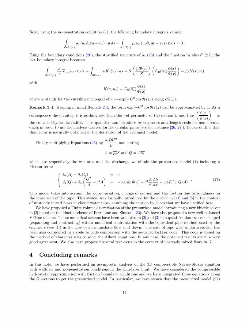
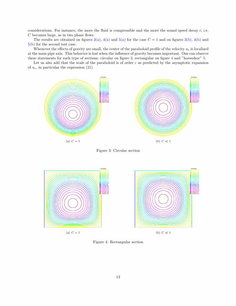
The results are obtained on figures 3(a), 4(a) and 5(a) for the case C = 1 and on figures 3(b), 4(b) and5(b) for the second test case.
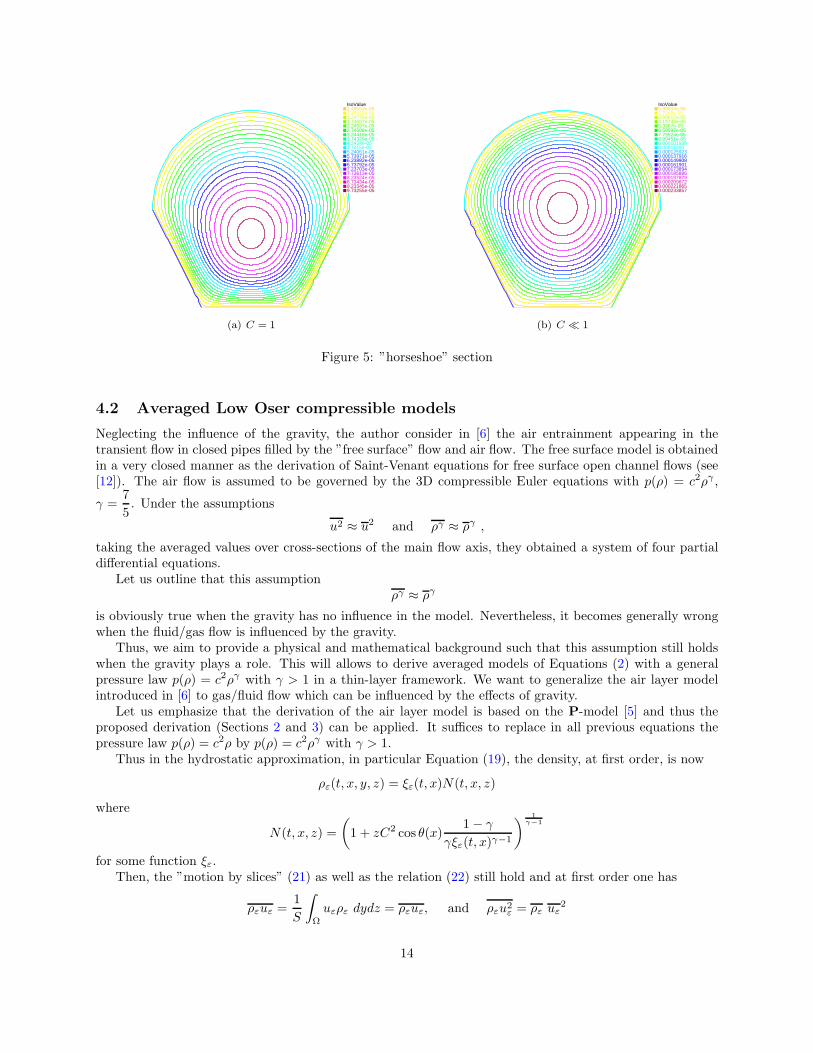
Whenever the effects of gravity are small, the center of the paraboloid profile of the velocity uε is localizedat the main pipe axis. This behavior is lost when the influence of gravity becomes important. One can observethese statements for each type of sections: circular on figure 3, rectangular on figure 4 and ”horseshoe” 5.
Let us also add that the scale of the paraboloid is of order ε as predicted by the asymptotic expansionof uε, in particular the expression (21).
Neglecting the influence of the gravity, the author consider in [6] the air entrainment appearing in thetransient flow in closed pipes filled by the ”free surface” flow and air flow. The free surface model is obtainedin a very closed manner as the derivation of Saint-Venant equations for free surface open channel flows (see[12]). The air flow is assumed to be governed by the 3D compressible Euler equations with p(ρ) = c2ργ ,
γ =7
5. Under the assumptions
u2 ≈ u2 and ργ ≈ ργ ,
taking the averaged values over cross-sections of the main flow axis, they obtained a system of four partialdifferential equations.
Let us outline that this assumptionργ ≈ ργ
is obviously true when the gravity has no influence in the model. Nevertheless, it becomes generally wrongwhen the fluid/gas flow is influenced by the gravity.
Thus, we aim to provide a physical and mathematical background such that this assumption still holdswhen the gravity plays a role. This will allows to derive averaged models of Equations (2) with a generalpressure law p(ρ) = c2ργ with γ > 1 in a thin-layer framework. We want to generalize the air layer modelintroduced in [6] to gas/fluid flow which can be influenced by the effects of gravity.
Let us emphasize that the derivation of the air layer model is based on the P-model [5] and thus theproposed derivation (Sections 2 and 3) can be applied. It suffices to replace in all previous equations thepressure law p(ρ) = c2ρ by p(ρ) = c2ργ with γ > 1.
Thus in the hydrostatic approximation, in particular Equation (19), the density, at first order, is now
ρε(t, x, y, z) = ξε(t, x)N(t, x, z)
where
N(t, x, z) =
(
1 + zC2 cos θ(x)1− γ
γξε(t, x)γ−1
)1
γ−1
for some function ξε.Then, the ”motion by slices” (21) as well as the relation (22) still hold and at first order one has
ρεuε =1
S
∫
Ω
uερε dydz = ρεuε, and ρεu2ε = ρε uε2
14
sinceρε(t, x) = ξε(t, x)N (t, x)
where
N(t, x) =1
S(x)
∫
Ω(x)
N(t, x, z) dy dz .
To go further in the derivation, if we integrate ργ along a section Ω we found that, even in the case γ = 2,at first order,
ρεγ ≇ ργε
Following Section 3 and keeping ργ , the resulting averaged model is
∂t(ρεS) + ∂x(ρεSuε) = 0
∂t(ρεSuε) + ∂x
(
ρεSuε2 +
1
M2a
ργεS
)
= −ρεSsin θ(x)
F 2L
+1
M2a
ργεdS
dx− ρεK(x, uε)
. (28)
This model is useless since it is a priori ill-posed due to the term ργε which cannot be determined from ρε.To make it usable one has to add an extra assumption in the asymptotic assumptions (16) concerning theOser number. Namely, if we assume that
C = O(εp) with p >1
2,
then, one hasN(t, x, z) = 1 +O(C2) = 1 +O(ε2p) .
Thus, the density is now approximated by
ρε = ξε +O(C2) = ξε +O(ε2p)
and we finally deduceργε = ξγε +O(C2) = ξγε +O(ε2p)
Thus, we obtain a class of averaged low Oser compressible models with γ > 1:
∂t(ξεS) + ∂x(ξεSu) = 0
∂t(ξεSuε) + ∂x
(
ξεSuε2 +
1
M2a
ξγε S
)
= −ξεSsin θ(x)
F 2L
+1
M2a
ξγεdS
dx− ξεK(x, uε)
(29)
as an approximation of order O(ε) of the Compressible Navier-Stokes equation (8) with wall-law and no-penetration boundary conditions. One can also consider the model (29) as an approximation of order O(C2)of the model (28). In view of Remark 3.1, let us note that this result also holds for γ = 1.
References
[1] A. Adamkowski, Analysis of transient flow in pipes with expanding or contracting sections, ASME J.of Fluid Engineering, 125 (2003), pp. 716–722.
[2] C. Bourdarias, M. Ersoy, and S. Gerbi, A kinetic scheme for pressurised flows in non uniform
closed water pipes, in Maths and water, Monogr. Real Acad. Ci. Exact. Fıs.-Quım. Nat. Zaragoza, 31,Real Acad. Ci. Exact., Fıs. Quım. Nat. Zar, Zaragoza, 2009, pp. 1–20.
[3] , A model for unsteady mixed flows in non uniform closed water pipes and a well-balanced finite
volume scheme, Int. J. Finite Vol., 6 (2009), p. 47.
15
[4] , A kinetic scheme for transient mixed flows in non uniform closed pipes: a global manner to
upwind all the source terms, J. Sci. Comput., 48 (2011), pp. 89–104.
[5] , A mathematical model for unsteady mixed flows in closed water pipes, Sci. China Math., 55 (2012),pp. 221–244.
[6] , Air entrainment in transient flows in closed water pipes: a two-layer approach, ESAIM Math.Model. Numer. Anal., 47 (2013), pp. 507–538.
[7] , A model for unsteady mixed flows in non uniform closed water pipes: a Full Kinetic Approach,Accepted in Numer. Math., (2014), p. 40.
[8] C. Bourdarias and S. Gerbi, A finite volume scheme for a model coupling free surface and pressurised
flows in pipes, J. Comp. Appl. Math., 209 (2007), pp. 109–131.
[9] H. Capart, X. Sillen, and Y. Zech, Numerical and experimental water transients in sewer pipes,Journal of Hydraulic Research, 35 (1997), pp. 659–672.
[10] N. T. Dong, Sur une methode numerique de calcul des ecoulements non permanents soit a surface
libre, soit en charge, soit partiellement a surface libre et partiellement en charge, La Houille Blanche, 2(1990), pp. 149–158.
[11] M. Ersoy, Modelisation, analyse mathematique et numerique de divers ecoulements compress-
ibles ou incompressibles en couche mince, PhD thesis, Universite de Savoie, 2010. available athttp://tel.archives-ouvertes.fr/tel-00529392.
[12] , A free surface model for incompressible pipe and open channel flow, (2013).
[13] M. Ersoy and T. Ngom, Existence of a global weak solution to compressible primitive equations, C.R. Math. Acad. Sci. Paris, 350 (2012), pp. 379–382.
[14] M. Ersoy, T. Ngom, and M. Sy, Compressible primitive equations: formal derivation and stability
of weak solutions, Nonlinearity, 24 (2011), pp. 79–96.
[15] S. Ferrari and F. Saleri, A new two-dimensional shallow water model including pressure effects and
[18] M. Hamam and A. McCorquodale, Transient conditions in the transition from gravity to surcharged
sewer flow, Can. J. Civ. Eng., 9 (1982), pp. 189–196.
[19] N. E. Kochin, On simplification of the equations of hydromechanics in the case of the general circulation
of the atmosphere, Trudy Glavn. Geofiz. Observator., 4 (1936), pp. 21–45.
[20] L. D. Landau and E. M. Lifshitz, Fluid mechanics, Translated from the Russian by J. B. Sykes andW. H. Reid. Course of Theoretical Physics, Vol. 6, Pergamon Press, London, 1959.
[21] F. Marche, Derivation of a new two-dimensional viscous shallow water model with varying topography,
bottom friction and capillary effects, European Journal of Mechanic. B, Fluids, 26 (2007), pp. 49–63.
[22] P. H. Oosthuizen and W. E. Carscallen, Compressible fluid flow, McGraw-Hill, New York, 1997.
[23] B. Perthame and C. Simeoni, A kinetic scheme for the Saint-Venant system with a source term,Calcolo, 38 (2001), pp. 201–231.
[24] P. Roe, Some contributions to the modelling of discontinuous flow, in Large-scale computations in fluidmechanics. Part 2. Proceedings of the fifteenth AMS-SIAM summer seminar on applied mathematicsheld at Scripps Institution of Oceanography, La Jolla, Calif., June 27-July 8, 1983, B. E. Engquist, S. Os-her, and R. C. J. Somerville, eds., vol. 22 of Lectures in Applied Mathematics, American MathematicalSociety, 1985, pp. 163–193.
[25] C. Song, J. Cardle, and K. Leung, Transient mixed-flow models for storm sewers, Journal ofHydraulic Engineering, ASCE, 109 (1983), pp. 1487–1503.
[26] V. Streeter and E. Wylie, Fluid Transients, McGraw-Hill, New York, 1978.