Available online at www.sciencedirect.com

ScienceDirect

Comput. Methods Appl. Mech. Engrg. 286 (2015) 1–21www.elsevier.com/locate/cma

A priori error estimation for the stochastic perturbation method

Xiang-Yu Wanga,b, Song Cena,d,e, C.F. Lib,c,∗, D.R.J. Owenb

a Department of Engineering Mechanics, School of Aerospace Engineering, Tsinghua University, Beijing 100084, Chinab Zienkiewicz Centre for Computational Engineering, College of Engineering, Swansea University, Swansea SA2 8PP, UK

c Energy Safety Research Institute, College of Engineering, Swansea University, Swansea SA2 8PP, UKd High Performance Computing Centre, School of Aerospace Engineering, Tsinghua University, Beijing 100084, Chinae Key Laboratory of Applied Mechanics, School of Aerospace Engineering, Tsinghua University, Beijing 100084, China

Received 30 June 2014; received in revised form 24 September 2014; accepted 28 November 2014Available online 16 December 2014

Abstract

The perturbation method has been among the most popular stochastic finite element methods due to its simplicity and efficiency.The error estimation for the perturbation method is well established for deterministic problems, but until now there has notbeen an error estimation developed in the probabilistic context. This paper presents a priori error estimation for the perturbationmethod in solving stochastic partial differential equations. The physical problems investigated here come from linear elasticity ofheterogeneous materials, where the material parameters are represented by stochastic fields. After applying the finite elementdiscretization to the physical problem, a stochastic linear algebraic equation system is formed with a random matrix on theleft hand side. Such systems have been efficiently solved by using the stochastic perturbation approach, without knowing howaccurate/inaccurate the perturbation solution is. In this paper, we propose a priori error estimation to directly link the error of thesolution vector with the variation of the source stochastic field. A group of examples are presented to demonstrate the effectivenessof the proposed error estimation.c⃝ 2014 Elsevier B.V. All rights reserved.

Keywords: Error estimation; Stochastic finite element methods; The perturbation method

1. Introduction

Over the past few decades, Stochastic Finite Element Methods (SFEM) have been developed for numerical analysisof uncertainty propagation in various engineering applications, in which the random factors can arise from thegeometry, the material properties or the boundary conditions. Unlike the conventional finite element method whichhas a well established theoretical framework, the SFEM has many different formulations, and these include the MonteCarlo method [1–4], the perturbation method [5–7], the Neumann expansion method [8,9], the polynomial chaosexpansion method [10–13], and the joint diagonalization method [14–16], among others. Despite these developments,little work has been done to address the error estimation of SFEMs. This work focuses on the error estimation of the

∗ Correspondence to: College of Engineering, Swansea University, Swansea SA2 8PP, UK.E-mail address: c.f.li@swansea.ac.uk (C.F. Li).

http://dx.doi.org/10.1016/j.cma.2014.11.0440045-7825/ c⃝ 2014 Elsevier B.V. All rights reserved.

2 X.-Y. Wang et al. / Comput. Methods Appl. Mech. Engrg. 286 (2015) 1–21

stochastic perturbation method. The basic idea and the development of the stochastic perturbation method is brieflyrecapped below. We also summarize the Monte Carlo method, which is taken as the reference for the error estimation.

The Monte Carlo method [1–4,17–19] generates samples for the source random variables involved, and corre-sponding to each sample a deterministic problem is solved to obtain the sample response, after which the statisticalevaluation is conducted on the whole set of sample responses. Among all SFEM approaches, the Monte Carlo ap-proach is the simplest and also the most versatile method. However, its computational cost is usually high and inmany cases, becomes unmanageable due to the limited computing resources available.

The basic idea of the stochastic perturbation method [5–7,20–22] is to expand the stochastic quantities by a Taylorexpansion, equate the items with the same order and calculate the responses. Due to the simplicity and efficiency of theperturbation method, it has been widely used in statics, thermodynamics, structural optimization, dynamics, etc. Changet al. [23] investigated the stochastic responses of geometrically nonlinear beams and frames, which have uncertainmaterial and geometric properties and are subjected to random excitations both spatially and temporally. Zhanget al. [24] analyzed the effects of random material properties on the elastic stability of structural members and frames.Lee et al. [25] presented an optimal design method to include the structural uncertainty. Kaminski et al. [26] appliedsecond order perturbation to homogenization problems. Lei et al. [27] presented an approach to analyze structureswith stochastic parameters under random excitation. Doltsinis et al. [28] discussed the robust design of structureswith stochastic parameters. Onkar et al. [29] proposed a method for the buckling analysis of both homogeneousand laminated plates with random material properties. Cavdar et al. [30] demonstrated an example of predicting theperformance of structural systems with uncertainties. Fan et al. [31] studied the robust optimization of large-scalespace structures under thermal loads. Guedri et al. [32] investigated uncertainty propagation for viscoelastic systems.Lepage et al. [33] applied the perturbation stochastic finite element method to the homogenization of polycrystallinematerials. Kaminski et al. [34] employed the perturbation-based stochastic finite elements to analyze compositematerials with stochastic interface defects, and later they [35] applied the generalized stochastic perturbation methodto thermal stresses and deformation analysis of spatial steel structures exposed to fire. In order to achieve betteraccuracy in the stochastic perturbation approach, Kaminski et al. [36,37] applied higher-order Taylor expansion andtested the procedure on simple problems with analytical solutions. Falsone et al. [38–40] developed a perturbation-like procedure for static and dynamic analysis of FE discretized structures with uncertainties, which overcomes thedrawbacks related to the standard perturbation approach.

Despite the wide use in various applications [25,26,28–35], the perturbation method does not have a rigorous errorestimation. Instead, the solution errors are usually examined by comparing with the Monte Carlo method. Purely basedon experience, some papers [6,22,36,41] suggested an applicable variation range of ten percent. Without rigorousproof, it is generally agreed that the perturbation method has very good efficiency and accuracy for small randomfluctuations, but the solution accuracy will decrease dramatically as the variation gets larger.

For error estimation, Oden et al. [42] provided a general error estimation for the error of the mathematical model,the error of numerical approximation, and the error of random fluctuation of the parameters, in which the variation ofthe parameters was approximated with the first order perturbation. A posteriori error estimation was derived. Babuskaet al. [43] studied the issues involved in the solution of linear ordinary differential equations with random parameters,and proved the existence of a rigorous error estimation for the perturbation method. However, the proposed errorestimation contains unknown constants which cannot be estimated either a priori or a posteriori. A similar work forlinear elliptic problems with random parameters was presented in [44], where the existence of the error estimationwas proved without providing a priori or a posteriori evaluation.

This work addresses the a priori error estimation for the stochastic partial differential equations commonlyencountered in stochastic finite element methods. The relative error is directly evaluated from the variation of thesource stochastic field. Section 2 explains the problem description and the general setup of a priori error estimation.In Sections 3 and 4, some preliminary theorems are first introduced, after which the detailed a priori estimation isderived. A series of numerical examples are given in Section 5 to demonstrate the effectiveness of the error estimation.Conclusions are given in Section 6.

2. Problem description

Using a stochastic finite element approach to solve problems associated with heterogeneous materials, the randommaterial property is usually described by a stochastic field which is modeled with the spectral representation [45,46],

X.-Y. Wang et al. / Comput. Methods Appl. Mech. Engrg. 286 (2015) 1–21 3

the Karhunen–Loeve (K–L) expansion [47,48] or the Fourier–Karhunen–Loeve (F–K–L) expansion [49,50]. Then,after applying the finite element discretization to the material domain, a set of linear stochastic equations can beconstructed with the following general form [6,15,16,44,47,51–54]:

(A0 + A1α1 + A2α2 + · · · + Amαm) u (ω) = f (ω)

(A0 + 1A) u (ω) = f (ω) ,(1)

where A0 is a n × n symmetric positive definite deterministic matrix, A1, . . . , Am are n × n symmetric deterministicmatrices, 1A = A1α1 + · · · + Amαm , ω denotes a random event, u (ω) is the unknown stochastic vector, f (ω) is aknown stochastic vector, and αi = αi (ω) are random variables, which can be correlated or uncorrelated. The exactsolution of Eq. (1) can be expressed as

u (ω) =

I +

i

αi A−10 Ai

−1

A−10 f (ω) = (I + B)−1 A−1

0 f (ω) , (2)

where B =

i αi A−10 Ai = A−1

0 1A.The above solution can then be approximated by using the perturbation method or the Neumann expansion method

[8,9]. It has been shown that the perturbation method and the Neumann expansion are essentially equivalent [44,55],because both methods can be derived from Taylor expansion. Corresponding to the kth order perturbation or Neumannexpansion, the approximate solution of Eq. (1) is

u (ω) =

I − B + B2

+ · · · + (−1)k Bk

A−10 f (ω) . (3)

In order to evaluate the error between the solution vectors u (ω) and u (ω), a vector norm is defined as follows:

∥u∥ ,

uTA0u =

uTC2u = ∥Cu∥2 (4)

where A0 = C2 and ∥·∥2 denotes the standard L2 norm for vectors. The corresponding matrix norm is defined as

∥S∥ ,CSCT

2, (5)

where S ∈ Rn×n . For consistency, the eigenvalues of A0 should be greater than 1. The new vector norm and the matrixnorm are verified in the Appendix.

From Eqs. (2) and (3), the following expressions hold with respect to the transformation matrix C:

Cu (ω) =

I +

i

αi C−1Ai C−1

−1

C−1f (ω) = (I + D)−1 C−1f (ω) (6)

Cu (ω) =

I − D + D2

+ · · · + (−1)k Dk

C−1f (ω) (7)

where D =

i αi C−1Ai C−1 is a symmetric matrix.Following Eqs. (2) and (3), the absolute error of the approximate solution is measured asu (ω) − u (ω)

=Cu (ω) − Cu (ω)

2

=

(I + D)−1−

I − D + D2

+ · · · + (−1)k Dk

C−1f (ω)

2

=

Dk+1 (I + D)−1 C−1f (ω)

2

=

Dk+1Cu (ω)

2

≤

Dk+1

2∥Cu (ω)∥2 =

Bk+1

2∥Cu (ω)∥2 = ρk+1

B ∥u (ω)∥ (8)

where ρB is the spectral radius of B. The relative error of the approximate solution is

RE =

u (ω) − u (ω)

∥u (ω)∥≤ ρk+1

B . (9)

4 X.-Y. Wang et al. / Comput. Methods Appl. Mech. Engrg. 286 (2015) 1–21

It should be noted that Eqs. (8) and (9) hold for any probabilistic distribution of random variables α1, α2, . . . , αm ,while ρB , the spectral radius of the random matrix B, varies corresponding to each sample.

3. Summary of related matrix algebra

The error estimation described in Eqs. (8) and (9) relies on ρB , the spectral radius of a random matrix, whichcannot be directly estimated. To make this more tractable, we will link ρB directly to the variation of the sourcerandom variables. We will show how this is achieved in Section 4, after introducing some preliminary theorems inthis section. The mathematical conclusions to be derived below are primarily based on the interlacing eigenvaluetheorem [56], which estimates the changes of eigenvalues of a symmetric matrix subjected to a perturbation.

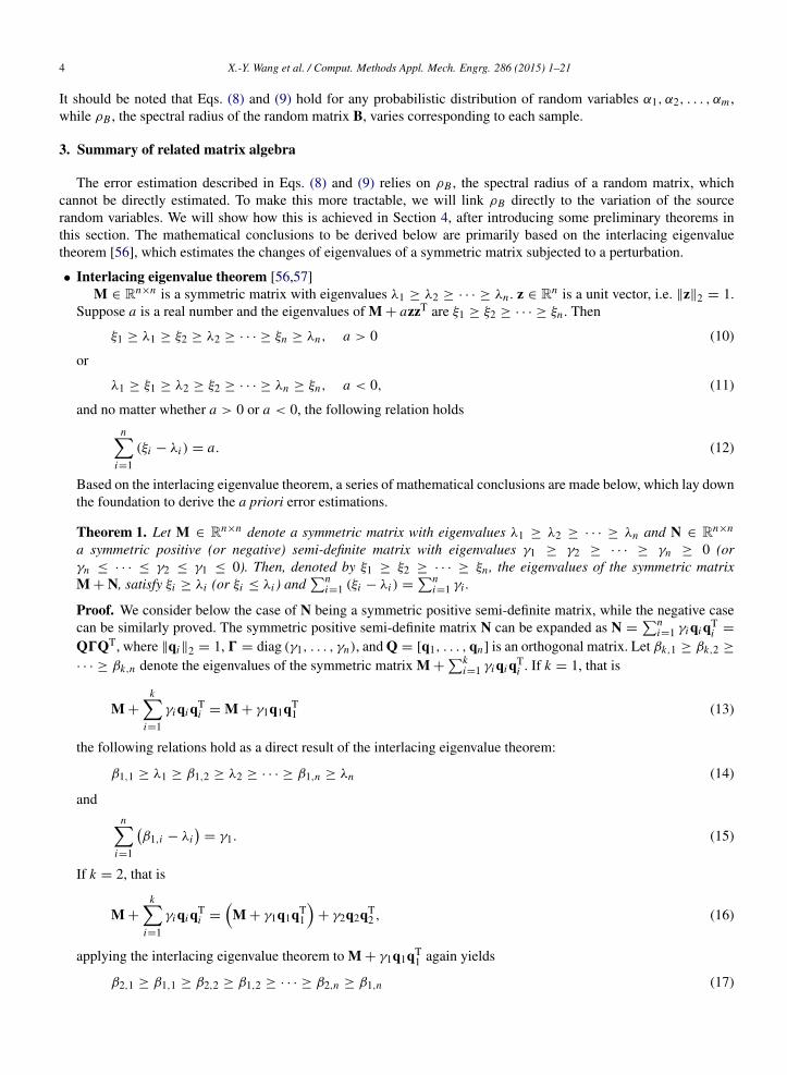
• Interlacing eigenvalue theorem [56,57]M ∈ Rn×n is a symmetric matrix with eigenvalues λ1 ≥ λ2 ≥ · · · ≥ λn . z ∈ Rn is a unit vector, i.e. ∥z∥2 = 1.

Suppose a is a real number and the eigenvalues of M + azzT are ξ1 ≥ ξ2 ≥ · · · ≥ ξn . Then

ξ1 ≥ λ1 ≥ ξ2 ≥ λ2 ≥ · · · ≥ ξn ≥ λn, a > 0 (10)

or

λ1 ≥ ξ1 ≥ λ2 ≥ ξ2 ≥ · · · ≥ λn ≥ ξn, a < 0, (11)

and no matter whether a > 0 or a < 0, the following relation holds

ni=1

(ξi − λi ) = a. (12)

Based on the interlacing eigenvalue theorem, a series of mathematical conclusions are made below, which lay downthe foundation to derive the a priori error estimations.

Theorem 1. Let M ∈ Rn×n denote a symmetric matrix with eigenvalues λ1 ≥ λ2 ≥ · · · ≥ λn and N ∈ Rn×n

a symmetric positive (or negative) semi-definite matrix with eigenvalues γ1 ≥ γ2 ≥ · · · ≥ γn ≥ 0 (orγn ≤ · · · ≤ γ2 ≤ γ1 ≤ 0). Then, denoted by ξ1 ≥ ξ2 ≥ · · · ≥ ξn , the eigenvalues of the symmetric matrixM + N, satisfy ξi ≥ λi (or ξi ≤ λi ) and

ni=1 (ξi − λi ) =

ni=1 γi .

Proof. We consider below the case of N being a symmetric positive semi-definite matrix, while the negative casecan be similarly proved. The symmetric positive semi-definite matrix N can be expanded as N =

ni=1 γi qi qT

i =

Q0QT, where ∥qi∥2 = 1, 0 = diag (γ1, . . . , γn), and Q = [q1, . . . , qn] is an orthogonal matrix. Let βk,1 ≥ βk,2 ≥

· · · ≥ βk,n denote the eigenvalues of the symmetric matrix M +k

i=1 γi qi qTi . If k = 1, that is

M +

ki=1

γi qi qTi = M + γ1q1qT

1 (13)

the following relations hold as a direct result of the interlacing eigenvalue theorem:

β1,1 ≥ λ1 ≥ β1,2 ≥ λ2 ≥ · · · ≥ β1,n ≥ λn (14)

andn

i=1

β1,i − λi

= γ1. (15)

If k = 2, that is

M +

ki=1

γi qi qTi =

M + γ1q1qT

1

+ γ2q2qT

2 , (16)

applying the interlacing eigenvalue theorem to M + γ1q1qT1 again yields

β2,1 ≥ β1,1 ≥ β2,2 ≥ β1,2 ≥ · · · ≥ β2,n ≥ β1,n (17)

X.-Y. Wang et al. / Comput. Methods Appl. Mech. Engrg. 286 (2015) 1–21 5

andn

i=1

β2,i − β1,i

= γ2. (18)

Repeating the above procedure yields

βk,1 ≥ βk−1,1 ≥ βk,2 ≥ βk−1,2 ≥ · · · ≥ βk,n ≥ βk−1,n (19)

andn

i=1

βk,i − βk−1,i

= γk . (20)

Then, it is straightforward to conclude

βn,1 ≥ βn−1,1 ≥ · · · ≥ β2,1 ≥ β1,1 ≥ λ1

βn,2 ≥ βn−1,2 ≥ · · · ≥ β2,2 ≥ β1,2 ≥ λ2

...

βn,n ≥ βn−1,n ≥ · · · ≥ β2,n ≥ β1,n ≥ λn

(21)

andn

i=1

βn,i − βn−1,i

+ · · · +

ni=1

β2,i − β1,i

+

ni=1

β1,i − λi

=

ni=1

βn,i − λi

=

ni=1

(ξi − λi )

=

ni=1

γi . (22)

When N is a symmetric negative semi-definite matrix, the corresponding conclusion can be similarly proved.

As the spectral radius is the maximum absolute value of eigenvalues, an inference is deduced from Theorem 1.

Inference 1. If M ∈ Rn×n is a symmetric matrix and its eigenvalues are arranged as λ1 ≥ λ2 ≥ · · · ≥ λn and|λ1| ≥ |λn| (or |λ1| ≤ |λn|), and N ∈ Rn×n is a symmetric positive (or negative) semi-definite matrix, thenρ (M + N) ≥ ρ (M) (or ρ (M + N) ≤ ρ (M)), where ρ (·) represents the spectral radius of a matrix.

Proof. We first consider N being a symmetric positive semi-definite matrix, with eigenvalues λ1 ≥ λ2 ≥ · · · ≥ λnand |λ1| ≥ |λn|. Following the same proof procedure as Theorem 1, it is easy to verify that

ρ (M + N) = βn,1 ≥ λ1 = max (|λ1| , |λn|) = ρ (M) . (23)

When N is a symmetric negative semi-definite matrix, the corresponding conclusion can be similarly proved.

Lemma 1. If H ∈ Rn×n is symmetric positive definite and H = S2, N ∈ Rn×n is positive (negative) semi-definite,then the eigenvalues of HN, SNS, NH are the same and SNS is positive (negative) semi-definite.

Proof. The following properties hold for a symmetric positive definite matrix H

H = P32PT= P3PTP3PT

= S2,

S = P3PT= ST

H−1= P3−1PTP3−1PT

= S−2,

(24)

where 3 is a diagonal matrix with positive entries.The eigenvalues of HN are defined as

det (HN − λI) = det

S2N − λI

= 0. (25)

6 X.-Y. Wang et al. / Comput. Methods Appl. Mech. Engrg. 286 (2015) 1–21

As S is positive definite, detS−1

and det (S) are nonzero. Eq. (25) can be written as

det

S−1

det

S2N − λI

det (S) = det (SNS − λI) = 0. (26)

Therefore, the eigenvalues of HN and SNS are the same. Similarly the eigenvalues of NH and SNS are the same.Let x denote an arbitrary nonzero vector. As S is positive definite, y = Sx is a nonzero vector. Therefore

xTSNSx =

STx

TN (Sx) = yTNy ≥ 0 (or ≤ 0) , (27)

i.e. SNS is positive (negative) semi-definite.

According to Lemma 1, the conclusions from Theorem 1 can be put in more generalized cases as describedbelow.

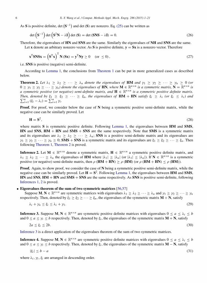
Theorem 2. Let λ1 ≥ λ2 ≥ · · · ≥ λn denote the eigenvalues of HM and γ1 ≥ γ2 ≥ · · · ≥ γn ≥ 0 (or0 ≥ γ1 ≥ γ2 ≥ · · · ≥ γn) denote the eigenvalues of HN, where M ∈ Rn×n is a symmetric matrix, N = Rn×n isa symmetric positive (or negative) semi-definite matrix, and H ∈ Rn×n is a symmetric positive definite matrix.Then, denoted by ξ1 ≥ ξ2 ≥ · · · ≥ ξn , the eigenvalues of HM + HN satisfy ξi ≥ λi (or ξi ≤ λi ) andn

i=1 (ξi − λi ) =n

i=1 γi .

Proof. For proof, we consider below the case of N being a symmetric positive semi-definite matrix, while thenegative case can be similarly proved. Let

H = S2, (28)

where matrix S is symmetric positive definite. Following Lemma 1, the eigenvalues between HM and SMS,HN and SNS, HM + HN and SMS + SNS are the same respectively. Note that SMS is a symmetric matrixand its eigenvalues are λ1 ≥ λ2 ≥ · · · ≥ λn ; SNS is a positive semi-definite matrix and its eigenvalues areγ1 ≥ γ2 ≥ · · · ≥ γn ≥ 0; SMS + SNS is a symmetric matrix and its eigenvalues are ξ1 ≥ ξ2 ≥ · · · ≥ ξn . Thenfollowing Theorem 1, Theorem 2 is proved.

Inference 2. Let M ∈ Rn×n denote a symmetric matrix, H ∈ Rn×n a symmetric positive definite matrix, andλ1 ≥ λ2 ≥ · · · ≥ λn the eigenvalues of HM where |λ1| ≥ |λn| (or |λ1| ≤ |λn|). If N ∈ Rn×n is a symmetricpositive (or negative) semi-definite matrix, then ρ (HM + HN) ≥ ρ (HM) (or ρ (HM + HN) ≤ ρ (HM)).

Proof. Again, to show proof, we consider the case of N being a symmetric positive semi-definite matrix, while thenegative case can be similarly proved. Let H = S2. Following Lemma 1, the eigenvalues between HM and SMS,HN and SNS, HM + HN and SMS + SNS are the same respectively. As SNS is positive semi-definite, followingInferences 1, 2 is proved.

• Eigenvalues theorem of the sum of two symmetric matrices [56,57]Suppose M, N ∈ Rn×n are symmetric matrices with eigenvalues λ1 ≥ λ2 ≥ · · · ≥ λn and γ1 ≥ γ2 ≥ · · · ≥ γn

respectively. Then, denoted by ξ1 ≥ ξ2 ≥ · · · ≥ ξn , the eigenvalues of the symmetric matrix M + N, satisfy

λi + γn ≤ ξi ≤ λi + γ1. (29)

Inference 3. Suppose M, N ∈ Rn×n are symmetric positive definite matrices with eigenvalues 0 ≤ a ≤ λi ≤ band 0 ≤ a ≤ γi ≤ b respectively. Then, denoted by ξi , the eigenvalues of the symmetric matrix M + N, satisfy

2a ≤ ξi ≤ 2b. (30)

Inference 3 is a direct application of the eigenvalues theorem of the sum of two symmetric matrices.

Inference 4. Suppose M, N ∈ Rn×n are symmetric positive definite matrices with eigenvalues 0 ≤ a ≤ λi ≤ band 0 ≤ a ≤ γi ≤ b respectively. Then, denoted by ξi , the eigenvalues of the symmetric matrix M − N, satisfy

|ξi | ≤ b − a (31)

where λi , γi , ξi are arranged in descending order.

X.-Y. Wang et al. / Comput. Methods Appl. Mech. Engrg. 286 (2015) 1–21 7

Proof. As the eigenvalues of N satisfy 0 ≤ a ≤ γi ≤ b, the eigenvalues of −N are −b ≤ γi ≤ −a ≤ 0. Accordingto the eigenvalues theorem of the sum of two symmetric matrices, the following relation holds

λi − b ≤ ξi ≤ λi − a. (32)

Then

b − b = λ1 − b ≤ ξ1 ≤ λ1 − a = b − a

a − b = λn − b ≤ ξn ≤ λn − a = a − a.(33)

Since ξ1 ≥ ξ2 ≥ · · · ≥ ξn , it can be concluded that |ξi | ≤ b − a.

Inference 5. Suppose M (ω) ∈ Rn×n is a random symmetric positive definite matrix with random eigenvalues0 ≤ a ≤ λi (ω) ≤ b. Then, denoted by ξi , the eigenvalues of the expectation matrix E (M (ω)), satisfy

a ≤ ξi ≤ b. (34)

Inference 5 is the random extension of Inference 3.

• The property of matrix eigenvaluesSuppose M ∈ Rn×n is a symmetric positive definite matrix, the corresponding eigenvalues are λ1 ≥ λ2 ≥ · · · ≥

λn > 0. Let e ∈ Rn denote a unit vector (∥e∥2 = 1), then

λn ∥e∥2 ≤ ∥Me∥2 ≤ λ1 ∥e∥2 . (35)

4. A priori error estimation

Based on the mathematical conclusions explained in the previous section, we derive below the a priori errorestimations for Eq. (1). Specifically, the unknown spectral radius ρB will be linked to the variation of source randomvariables, which can be directly estimated a priori.

4.1. Spectral radius of the stiffness matrix for random media

In continuum mechanics, the material properties are, in the most general case, represented by a 4-th order tensor,the constitutive tensor. This is also true for random media whose material properties are represented by stochasticfields. For the sake of simplicity, an elastostatic problem with a random elastic modulus E (x, ω) is considered hereto illustrate the formulation, while the general concept applies to other types of problems and the general constitutivetensor as well. No matter how the stochastic field E (x, ω) is quantified, i.e. by the spectral representation [45,46], theK–L expansion [47,48] or the F–K–L expansion [49,50], its general form is

E (x, ω) = E0 (x) + 1E (x, ω) , (36)

where E0 (x) is the expectation of the elastic modulus, and 1E (x, ω) denotes its random part. Following a finiteelement discretization, the stiffness matrices A0 and 1A in Eq. (1) can be expressed as

A0 =

i

E0 (x) Kei , (37)

1A =

i

1Ei (x, ω) Kei , (38)

where Kei denotes the i th element stiffness matrix without inclusion of the elastic modulus.

Theorem 3 describes the relation between the variation range of the stochastic field and the spectral radius ρBdefined in Eq. (8).

Theorem 3 (Spectral Radius Theorem for Random Stiffness Matrix). Define

maxE =max (|1E (x, ω)|)

min (E0 (x))=

max (|E (x, ω) − E0 (x)|)

min (E0 (x)), (39)

8 X.-Y. Wang et al. / Comput. Methods Appl. Mech. Engrg. 286 (2015) 1–21

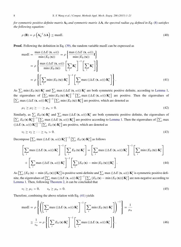
for symmetric positive definite matrix A0 and symmetric matrix 1A, the spectral radius ρB defined in Eq. (8) satisfiesthe following equation:

ρ (B) = ρ

A−10 1A

≤ maxE. (40)

Proof. Following the definition in Eq. (39), the random variable maxE can be expressed as

maxE =max (|1E (x, ω)|)

min (E0 (x))= ρ

max (|1E (x, ω)|)

min (E0 (x))I

= ρ

max (|1E (x, ω)|)

min (E0 (x))

i

Kei

−1 i

Kei

= ρ

i

min (E0 (x)) Kei

−1 i

max (|1E (x, ω)|) Kei

. (41)

As

i min (E0 (x)) Kei and

i max (|1E (x, ω)|) Ke

i are both symmetric positive definite, according to Lemma 1,

the eigenvalues of

i min (E0 (x)) Kei

−1 i max (|1E (x, ω)|) Ke

i

are positive. Then the eigenvalues of

i max (|1E (x, ω)|) Kei

−1 i min (E0 (x)) Ke

i

are positive, which are denoted as

µ1 ≥ µ2 ≥ · · · ≥ µn > 0. (42)

Similarly, as

i E0 (x) Kei and

i max (|1E (x, ω)|) Ke

i are both symmetric positive definite, the eigenvalues ofi E0 (x) Ke

i

−1 i max (|1E (x, ω)|) Ke

i

are positive according to Lemma 1. Then the eigenvalues of

i max

(|1E (x, ω)|) Kei

−1 i E0 (x) Ke

i

are positive, which are denoted as

ν1 ≥ ν2 ≥ · · · ≥ νn > 0. (43)

Decompose

i max (|1E (x, ω)|) Kei

−1 i E0 (x) Ke

i

as follows

i

max (|1E (x, ω)|) Kei

−1 i

E0 (x) Kei

=

i

max (|1E (x, ω)|) Kei

−1 i

min (E0 (x)) Kei

+

i

max (|1E (x, ω)|) Kei

−1 i

[E0 (x) − min (E0 (x))] Kei

. (44)

As

i [E0 (x) − min (E0 (x))] Kei

is positive semi-definite and

i max (|1E (x, ω)|) Ke

i is symmetric positive defi-

nite, the eigenvalues of

i max (|1E (x, ω)|) Kei

−1 i [E0 (x) − min (E0 (x))] Ke

i

are non-negative according to

Lemma 1. Then, following Theorem 2, it can be concluded that

ν1 ≥ µ1 > 0, νn ≥ µn > 0. (45)

Therefore, combining the above relation with Eq. (41) yields

maxE = ρ

i

max (|1E (x, ω)|) Kei

−1 i

min (E0 (x)) Kei

−1 =

1µn

≥1νn

= ρ

i

E0 (x) Kei

−1 i

max (|1E (x, ω)|) Kei

. (46)

X.-Y. Wang et al. / Comput. Methods Appl. Mech. Engrg. 286 (2015) 1–21 9

As

i E0 (x) Kei and

i max (|1E (x, ω)|) Ke

i are both positive definite, the eigenvalues of

i E0 (x) Kei

−1i max (|1E (x, ω)|) Ke

i

are non-negative according to Lemma 1, which are denoted as

maxE ≥ ξ1 ≥ ξ2 ≥ · · · ≥ ξn ≥ 0. (47)

Decompose

i E0 (x) Kei

−1 i max (|1E (x, ω)|) Ke

i

as follows

i

E0 (x) Kei

−1 i

max (|1E (x, ω)|) Kei

=

i

E0 (x) Kei

−1 i

1Ei (x, ω) Kei

+

i

E0 (x) Kei

−1 i

[max (|1E (x, ω)|) − 1Ei (x, ω)] Kei

. (48)

As

i [max (|1E (x, ω)|) − 1Ei (x, ω)] Kei is positive semi-definite and

i E0 (x) Ke

i is positive definite, the eigen-

values of

i E0 (x) Kei

−1 i [max (|1E (x)|) − 1Ei (x)] Ke

i

are non-negative according to Lemma 1. Let

λ1 ≥ λ2 ≥ · · · ≥ λn (49)

denote the eigenvalues of

i E0 (x) Kei

−1 i 1Ei (x, ω) Ke

i

. Following Theorem 2, it can be concluded that

maxE ≥ ξ1 ≥ λ1, maxE ≥ ξn ≥ λn . (50)

Now we decompose

i E0 (x) Kei

−1 i 1Ei (x, ω) Ke

i

into

i

E0 (x) Kei

−1 i

1Ei (x, ω) Kei

= −

i

E0 (x) Kei

−1 i

max (|1E (x, ω)|) Kei

+

i

E0 (x) Kei

−1 i

[max (|1E (x, ω)|) + 1Ei (x, ω)] Kei

. (51)

As

i [max (|1E (x, ω)|) + 1Ei (x, ω)] Kei is positive semi-definite and

i E0 (x) Ke

i is positive definite, the eigen-

values of

i E0 (x) Kei

−1 i [max (|1E (x, ω)|) + 1Ei (x, ω)] Ke

i

are non-negative according to Lemma 1. Fol-

lowing Eq. (47), the eigenvalues of −

i E0 (x) Kei

−1 i max (|1E (x, ω)|) Ke

i

are

0 ≥ −ξn ≥ · · · ≥ −ξ2 ≥ −ξ1 ≥ −maxE. (52)

Applying Theorem 2 to Eq. (51) yields

λ1 ≥ −ξn ≥ −maxE, λn ≥ −ξ1 ≥ −maxE. (53)

Combining Eqs. (50) and (53) yields

maxE ≥ ξ1 ≥ λ1 ≥ −ξn ≥ −maxE

maxE ≥ ξn ≥ λn ≥ −ξ1 ≥ −maxE.(54)

Therefore,

ρ (B) = ρ

A−10 1A

= ρ

i

E0 (x) Kei

−1 i

1Ei (x, ω) Kei

= max (|λ1| , |λn|) ≤ maxE. (55)

Remark of Theorem 3. It should be noted that the stochastic parameter in Theorem 3 must have a linear relation withthe “element stiffness matrix”, such as the elastic modulus or the thermal conductivity. Meanwhile the deterministicpart or the expectation part of the overall “stiffness matrix” needs to be positive definite. However, the elastic modulusor the thermal conductivity itself can be nonlinear. Theorem 3 does not hold for stochastic parameters that arenonlinear with respect to the element stiffness matrix, e.g. Poisson’s ratio. In these cases, it may be possible to

10 X.-Y. Wang et al. / Comput. Methods Appl. Mech. Engrg. 286 (2015) 1–21

introduce a transformation to the relevant material parameter such that a similar conclusion can still hold, but thisis outside the scope of the current work.

4.2. A priori error estimation for the stochastic perturbation method

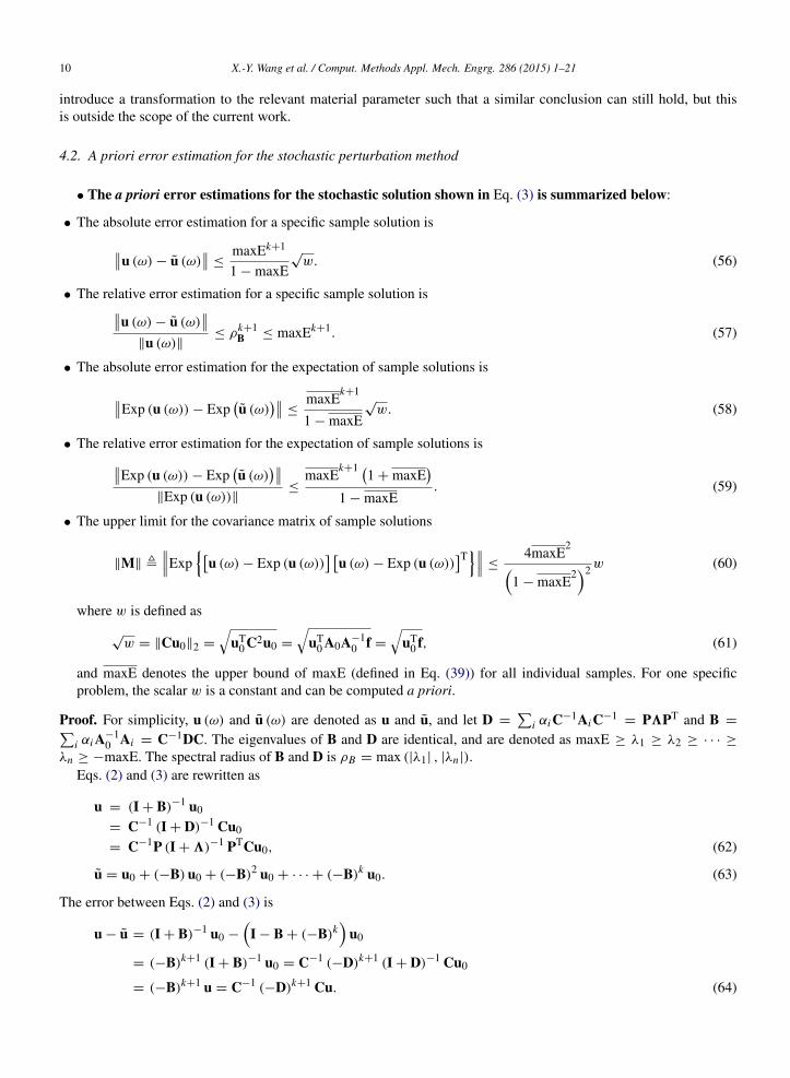
• The a priori error estimations for the stochastic solution shown in Eq. (3) is summarized below:

• The absolute error estimation for a specific sample solution isu (ω) − u (ω) ≤

maxEk+1

1 − maxE

√w. (56)

• The relative error estimation for a specific sample solution isu (ω) − u (ω)

∥u (ω)∥≤ ρk+1

B ≤ maxEk+1. (57)

• The absolute error estimation for the expectation of sample solutions is

Exp (u (ω)) − Expu (ω)

≤maxE

k+1

1 − maxE

√w. (58)

• The relative error estimation for the expectation of sample solutions isExp (u (ω)) − Expu (ω)

∥Exp (u (ω))∥

≤maxE

k+1 1 + maxE

1 − maxE

. (59)

• The upper limit for the covariance matrix of sample solutions

∥M∥ ,Exp

u (ω) − Exp (u (ω))

u (ω) − Exp (u (ω))

T ≤4maxE

21 − maxE

22 w (60)

where w is defined as

√w = ∥Cu0∥2 =

uT

0 C2u0 =

uT

0 A0A−10 f =

uT

0 f, (61)

and maxE denotes the upper bound of maxE (defined in Eq. (39)) for all individual samples. For one specificproblem, the scalar w is a constant and can be computed a priori.

Proof. For simplicity, u (ω) and u (ω) are denoted as u and u, and let D =

i αi C−1Ai C−1= P3PT and B =

i αi A−10 Ai = C−1DC. The eigenvalues of B and D are identical, and are denoted as maxE ≥ λ1 ≥ λ2 ≥ · · · ≥

λn ≥ −maxE. The spectral radius of B and D is ρB = max (|λ1| , |λn|).Eqs. (2) and (3) are rewritten as

u = (I + B)−1 u0

= C−1 (I + D)−1 Cu0

= C−1P (I + 3)−1 PTCu0, (62)

u = u0 + (−B) u0 + (−B)2 u0 + · · · + (−B)k u0. (63)

The error between Eqs. (2) and (3) is

u − u = (I + B)−1 u0 −

I − B + (−B)k

u0

= (−B)k+1 (I + B)−1 u0 = C−1 (−D)k+1 (I + D)−1 Cu0

= (−B)k+1 u = C−1 (−D)k+1 Cu. (64)

X.-Y. Wang et al. / Comput. Methods Appl. Mech. Engrg. 286 (2015) 1–21 11

• The absolute error estimation for a specific sample solutionu − u =

C−1 (−D)k+1 (I + D)−1 Cu0

=

(−D)k+1 (I + D)−1 Cu0

2. (65)

As the vector norm and matrix norm defined in Eqs. (4) and (5) are consistent, the following relation holds:u − u ≤

Dk+1 (I + D)−1

2∥Cu0∥2 =

3k+1 (I + 3)−1

2∥Cu0∥2

= max λi

1 + λi

√w =

maxEk+1

1 − maxE

√w. (66)

• The relative error estimation for a specific sample solutionu − u

∥u∥=

C−1 (−D)k+1 Cu

∥u∥=

(−D)k+1 Cu

2

∥Cu∥2

≤

(−D)k+1

2 ∥Cu∥2

∥Cu∥2=

(−D)k+1

2

= ρk+1B ≤ maxEk+1. (67)

• The absolute error estimation for the expectation of sample solutionsFollowing Eq. (93), the following relation holdsExp (u) − Exp

u =

Expu − u

≤ Expu − u

, (68)

where Exp ( ) denotes the mathematical expectation. Substituting Eq. (66) into Eq. (68) yields

Exp (u) − Expu ≤ Exp

maxE

k+1

1 − maxE

√w

=

maxEk+1

1 − maxE

√w. (69)

• The relative error estimation for the expectation of sample solutionsThe relative error estimation for the expectation of sample solutions isExp (u) − Exp

u

∥Exp (u)∥=

Expu − u

∥Exp (u)∥

=

ExpC−1 (−D)k+1 (I + D)−1 Cu0

ExpC−1 (I + D)−1 Cu0

=

Exp(−D)k+1 (I + D)−1 Cu0

2Exp

(I + D)−1 Cu0

2

=

Exp(−D)k+1 (I + D)−1 (Cu0)

2Exp

(I + D)−1 (Cu0)

2

. (70)

Denoted by λ(I+D)−1 and λ(I+3)−1 , the eigenvalues of (I + D)−1 and (I + 3)−1 satisfy

11 + maxE

≤ λ(I+D)−1 = λ(I+3)−1 ≤1

1 − maxE. (71)

According to Inference 5, the following relation holds

1

1 + maxE≤ λExp(I+D)−1 ≤

1

1 − maxE. (72)

Let y , Cu0 = ∥y∥2 ey, thenExp(I + D)−1

(Cu0)

2

=

Exp(I + D)−1

∥y∥2 ey

2

= ∥y∥2

Exp(I + D)−1

ey

2. (73)

Applying Eq. (35) to the above equation yieldsExp(I + D)−1

(Cu0)

2

≥ ∥y∥2

ey

2 min λExp(I+D)−1 . (74)

12 X.-Y. Wang et al. / Comput. Methods Appl. Mech. Engrg. 286 (2015) 1–21

Then, according to Eq. (72), the denominator of Eq. (70) satisfies the following lower boundExp(I + D)−1

(Cu0)

2

≥1

1 + maxE∥y∥2 =

1

1 + maxE∥Cu0∥2 . (75)

For the nominator in Eq. (70), the following relation holdsExp(−D)k+1 (I + D)−1

(Cu0)

2

≤

Exp(−D)k+1 (I + D)−1

2∥Cu0∥2

≤ Exp(−D)k+1 (I + D)−1

2

∥Cu0∥2

= Exp(−3)k+1 (I + 3)−1

2

∥Cu0∥2

= Exp

max λk+1

1 + λ

∥Cu0∥2

=maxE

k+1

1 − maxE∥Cu0∥2 . (76)

Substituting Eqs. (75) and (76) into Eq. (70) yieldsExp (u) − Expu

∥Exp (u)∥≤

maxEk+1

1−maxE∥Cu0∥2

11+maxE

∥Cu0∥2=

maxEk+1

1 + maxE

1 − maxE. (77)

• The upper limit for the covariance matrix of sample solutionsThe covariance matrix of sample solutions is

∥M∥ =

Exp

u − Exp (u)

u − Exp (u)T . (78)

Following Eq. (93), the following relation holds

∥M∥ ≤ Expu − Exp (u)

u − Exp (u)

T ≤ Expu − Exp (u)

2

= ExpC−1 (I + D)−1 Cu0 − Exp

C−1 (I + D)−1 Cu0

2

= Exp(I + D)−1 Cu0 − Exp

(I + D)−1 Cu0

2

2

≤ Exp(I + D)−1

− Exp (I + D)−12

2

∥Cu0∥

22

≤ max(I + D)−1

− Exp (I + D)−12

2

∥Cu0∥

22 . (79)

Then, according to Eqs. (71), (72) and Inference 4, the upper bound of the covariance matrix can be estimated as

∥M∥ ≤ max

max λ(I+D)−1 − min λExp(I+D)−1

2

∥Cu0∥22

= max

1

1 − maxE−

1

1 + maxE

2

∥Cu0∥22

=4maxE

21 − maxE

22 w. (80)

Remark. Eq. (57) can be applied to estimate the relative errors of the stochastic perturbation method, no matterwhether the right hand side is stochastic or not. If the zero order perturbation is applied, that is, the stochastic field

X.-Y. Wang et al. / Comput. Methods Appl. Mech. Engrg. 286 (2015) 1–21 13

Fig. 1. Stretching of a bar with random elastic modulus.

is approximated by its expectation, then RE =∥u−u∥

∥u∥≤ ρB ≤ maxE. This means that if heterogeneous materials

are treated as homogeneous ones, of which the relative variation magnitude is maxE, then the relative error of thesolution is maxE. Note that the zero order perturbation is the same as the homogenization procedure of heterogeneousmaterials in this case.

5. Numerical examples

The error estimation derived above is mathematically rigorous. Some illustrative examples are presented in thissection to demonstrate the use of the a priori error estimation.

Let RE =∥u(ω)−u(ω)∥

∥u(ω)∥, then Eq. (57) can be rewritten as follows

ln (RE) ≤ (k + 1) ln (maxE) . (81)

Eq. (81) represents the relation between the relative error of a specific sample solution and the maximum variationrange of the random elastic modulus. In all examples presented in this section, the third order perturbation solution isadopted. Therefore, Eq. (81) becomes

ln (RE) ≤ 4 ln (maxE) . (82)

To show the statistics of the error, 5000 sample solutions are calculated for each example case. Gaussian and uniformvariables are taken as examples. Note that Gaussian random variables take values in the entire real number set,but the elastic modulus of any practical material can only vary in a specific range. Therefore, when the Gaussiandistribution with standard deviation σ and expectation E0 is used to approximate the real-world elastic modulus, weset maxE = 3σ , which confines the elastic modulus to the interval [E0 − 3σ E0, E0 + 3σ E0] with the probabilityof 97.3%. In the uniform distribution case, the standard deviation and expectation of the material elastic modulusare σ/

√3 and E0 respectively. Therefore the variation range of the elastic modulus is [E0 − σ E0, E0 + σ E0], and

maxE = σ .

Example 1. As Fig. 1 shows, a straight bar has ten consecutive sections with the same geometry (length and crosssection) but different elastic moduli. The length of the whole bar is 1.0 m, and the cross section area is 4.0 × 10−4 m2.The bar is fixed at the left end and stretched at the right end. The elastic moduli of these bar sections are modeled asindependent random variables with Gaussian or uniform distribution, whose expectation is 2.0 × 1011 Pa. In the finiteelement discretization, each bar section is represented by one element so that there are ten elements along the totallength.

Case 1: The ten elastic moduli are assumed to be Gaussian random variables, with a standard deviation of σ = 1/30or equally the variation range [0.9E0, 1.1E0]. The relation between the relative error and the maximum variation rangeis shown in Fig. 2.

Case 2: The ten elastic moduli are assumed to be uniformly distributed with a standard deviation of σ = 0.1/√

3 orequally the variation range [0.9E0, 1.1E0]. The relation between the relative error and the maximum variation rangeis shown in Fig. 3.

Case 3: The ten elastic moduli are assumed to be uniformly distributed with a standard deviation of σ = 0.4/√

3 orequally the variation range [0.6E0, 1.4E0]. The relation between the relative error and the maximum variation rangeis shown in Fig. 4.

The results shown in Figs. 2–4 all confirm that the error estimation is correct. Moreover, Figs. 2 and 3 show thatthe error estimation is effective regardless of the distributions of source random variables. The results shown in Figs. 3

14 X.-Y. Wang et al. / Comput. Methods Appl. Mech. Engrg. 286 (2015) 1–21

-5

-10

-15

-20

-25-22 -20 -18 -16 -14 -12 -10 -8 -6

Fig. 2. The relation between the relative error and the variation range (Case 1).

-6

-8

-10

-14

-12

-16-16 -15 -14 -13 -12 -11 -10 -8-9 -7

Fig. 3. The relation between the relative error and the variation range (Case 2).

Fig. 4. The relation between the relative error and the variation range (Case 3).

and 4 confirm that the error estimation applies to both small and large variations. With these results, the followingexamples will only use Gaussian distributions for conciseness.

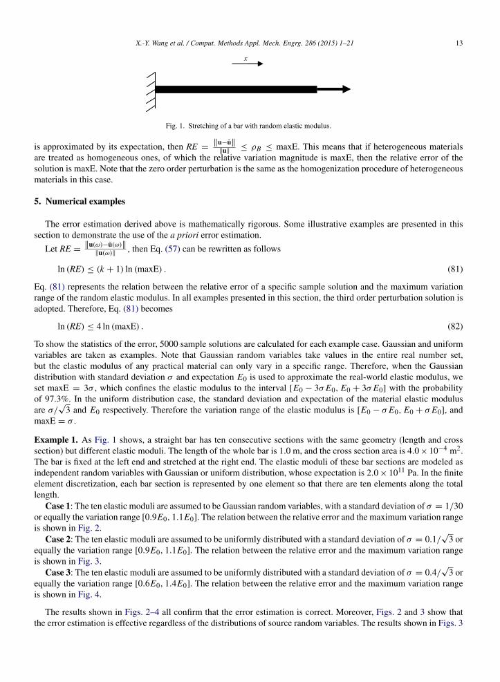
Example 2. A truss system is analyzed as depicted in Fig. 5. The length of each truss member is 1.0 m, and thecross section area is 4.0 × 10−4 m2. Each truss member is discretized as one element and the elastic modulus of each

X.-Y. Wang et al. / Comput. Methods Appl. Mech. Engrg. 286 (2015) 1–21 15

Fig. 5. A truss structure with random elastic modulus for each truss member.

Fig. 6. The relation between the relative error and the variation range.

member is an independent Gaussian random variable with the expectation of 2.0 × 1011 Pa and the standard deviationof σ = 1/10 or equally the variation range [0.7E0, 1.3E0]. The relation between the relative error and the maximumvariation range is shown in Fig. 6, which also confirms the correctness of the error estimation.

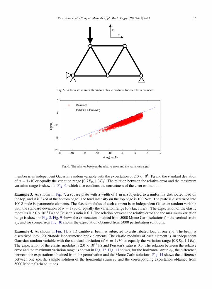
Example 3. As shown in Fig. 7, a square plate with a width of 1 m is subjected to a uniformly distributed load onthe top, and it is fixed at the bottom edge. The load intensity on the top edge is 100 N/m. The plate is discretized into100 8-node isoparametric elements. The elastic modulus of each element is an independent Gaussian random variablewith the standard deviation of σ = 1/30 or equally the variation range [0.9E0, 1.1E0]. The expectation of the elasticmodulus is 2.0×1011 Pa and Poisson’s ratio is 0.3. The relation between the relative error and the maximum variationrange is shown in Fig. 8. Fig. 9 shows the expectation obtained from 5000 Monte Carlo solutions for the vertical strainεy , and for comparison Fig. 10 shows the expectation obtained from 5000 perturbation solutions.

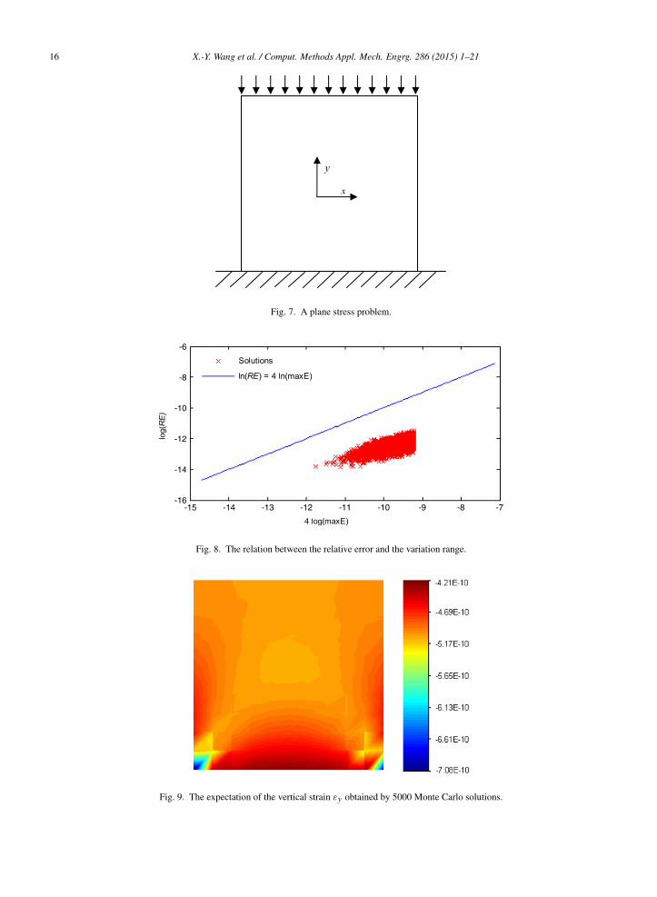
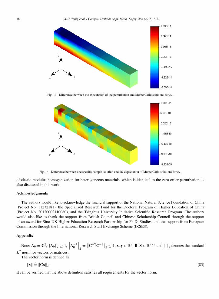
Example 4. As shown in Fig. 11, a 3D cantilever beam is subjected to a distributed load at one end. The beam isdiscretized into 120 20-node isoparametric brick elements. The elastic modulus of each element is an independentGaussian random variable with the standard deviation of σ = 1/30 or equally the variation range [0.9E0, 1.1E0].The expectation of the elastic modulus is 2.0 × 1011 Pa and Poisson’s ratio is 0.3. The relation between the relativeerror and the maximum variation range is shown in Fig. 12. Fig. 13 shows, for the horizontal strain εx , the differencebetween the expectations obtained from the perturbation and the Monte Carlo solutions. Fig. 14 shows the differencebetween one specific sample solution of the horizontal strain εx and the corresponding expectation obtained from5000 Monte Carlo solutions.

16 X.-Y. Wang et al. / Comput. Methods Appl. Mech. Engrg. 286 (2015) 1–21

Fig. 7. A plane stress problem.

-6

-8

-10

-14

-12

-16-15 -14 -13 -12 -11 -10 -8-9 -7

Fig. 8. The relation between the relative error and the variation range.

Fig. 9. The expectation of the vertical strain εy obtained by 5000 Monte Carlo solutions.

X.-Y. Wang et al. / Comput. Methods Appl. Mech. Engrg. 286 (2015) 1–21 17

Fig. 10. The expectation of the vertical strain εy obtained by 5000 perturbation solutions.

Fig. 11. A 3D cantilever beam.

-6

-8

-10

-14

-12

-16-15 -14 -13 -12 -11 -10 -8-9 -7

Fig. 12. The relation between the relative error and the variation range.

6. Conclusions

For the first time, a priori error estimation is established for the stochastic perturbation method. The mathematicallyrigorous result is derived for the linear stochastic equations commonly encountered in stochastic finite elementmethods. Specifically, the error of the solution vector is directly linked to the variation range of the source stochasticfields, which can be computed a priori. Although the result is presented for examples with random elastic modulus,the concept is applicable to other more general cases, where the material parameter is linear with respect to the elementstiffness matrix and the deterministic part (i.e. the expectation part) of the stiffness matrix is positive definite. The error

18 X.-Y. Wang et al. / Comput. Methods Appl. Mech. Engrg. 286 (2015) 1–21

Fig. 13. Difference between the expectation of the perturbation and Monte Carlo solutions for εx .

Fig. 14. Difference between one specific sample solution and the expectation of Monte Carlo solutions for εx .

of elastic-modulus homogenization for heterogeneous materials, which is identical to the zero order perturbation, isalso discussed in this work.

Acknowledgments

The authors would like to acknowledge the financial support of the National Natural Science Foundation of China(Project No. 11272181), the Specialized Research Fund for the Doctoral Program of Higher Education of China(Project No. 20120002110080), and the Tsinghua University Initiative Scientific Research Program. The authorswould also like to thank the support from British Council and Chinese Scholarship Council through the supportof an award for Sino-UK Higher Education Research Partnership for Ph.D. Studies, and the support from EuropeanCommission through the International Research Staff Exchange Scheme (IRSES).

Appendix

Note: A0 = C2, ∥A0∥2 ≥ 1,A−1

0

2

=C−TC−1

2 ≤ 1, x, y ∈ Rn , R, S ∈ Rn×n and ∥·∥2 denotes the standard

L2 norm for vectors or matrices.The vector norm is defined as

∥x∥ , ∥Cx∥2 . (83)

It can be verified that the above definition satisfies all requirements for the vector norm:

X.-Y. Wang et al. / Comput. Methods Appl. Mech. Engrg. 286 (2015) 1–21 19

1. The positive property

∥x∥ = ∥Cx∥2 ≥ 0. (84)

2. The linear property

∥ax∥ = ∥aCx∥2 = a ∥Cx∥2 = a ∥x∥ , a > 0. (85)

3. The inequality of sum

∥x + y∥ = ∥C (x + y)∥2 = ∥Cx + Cy∥2 ≤ ∥Cx∥2 + ∥Cy∥2 = ∥x∥ + ∥y∥ . (86)

The matrix norm is defined as

∥S∥ ,CSCT

2. (87)

It can be verified that the above definition satisfies all requirements for the matrix norm:

1. The positive property

∥S∥ =

CSCT

2≥ 0. (88)

2. The linear property

∥aS∥ =

aCSCT

2= a

CSCT

2= a ∥S∥ , a > 0. (89)

3. The inequality of sum

∥R + S∥ =

C (R + S) CT

2=

CRCT+ CSCT

2

≤

CRCT

2+

CSCT

2= ∥R∥ + ∥S∥ . (90)

4. The inequality of product

∥RS∥ =

CRSCT

2=

CRCTC−TC−1CSCT

2

≤

CRCT

2

C−TC−1

2

CSCT

2≤ ∥R∥ ∥S∥ . (91)

5. Consistence of vector norm and matrix norm

∥Sx∥ = ∥CSx∥2 =

CSCTC−TC−1Cx

2

≤

CSCT

2

C−TC−1

2∥Cx∥2

≤ ∥S∥ ∥x∥ . (92)

It is straightforward to confirm that the expectations of the norms defined in Eqs. (83) and (88) satisfy

∥Exp (x)∥ =

n

i=1x

n

=1n

ni=1

x

≤1n

ni=1

∥x∥ = Exp (∥x∥)

∥Exp (S)∥ =

n

i=1S

n

=1n

ni=1

S

≤1n

ni=1

∥S∥ = Exp (∥S∥) .

(93)

20 X.-Y. Wang et al. / Comput. Methods Appl. Mech. Engrg. 286 (2015) 1–21

References

[1] M. Shinozuka, Structural response variability, J. Eng. Mech. 113 (1987) 825–842.[2] S.K. Au, J.L. Beck, Estimation of small failure probabilities in high dimensions by subset simulation, Probab. Eng. Mech. 16 (2001) 263–277.[3] S. Au, J. Beck, Subset simulation and its application to seismic risk based on dynamic analysis, J. Eng. Mech. 129 (2003) 901–917.[4] G.I. Schueller, H.J. Pradlwarter, P.S. Koutsourelakis, A critical appraisal of reliability estimation procedures for high dimensions, Probab.

Eng. Mech. 19 (2004) 463–474.[5] E. Vanmarcke, M. Grigoriu, Stochastic finite element analysis of simple beams, J. Eng. Mech. 109 (1983) 1203–1214.[6] W.K. Liu, T. Belytschko, A. Mani, Random field finite-elements, Internat. J. Numer. Methods Engrg. 23 (1986) 1831–1845.[7] W.K. Liu, T. Belytschko, A. Mani, Probabilistic finite elements for nonlinear structural dynamics, Comput. Methods Appl. Mech. Engrg. 56

(1986) 61–81.[8] M. Shinozuka, G. Deodatis, Response variability of stochastic finite-element systems, J. Eng. Mech.—ASCE 114 (1988) 499–519.[9] F. Yamazaki, M. Shinozuka, G. Dasgupta, Neumann expansion for stochastic finite-element analysis, J. Eng. Mech.—ASCE 114 (1988)

1335–1354.[10] T. Crestaux, O. Le Maitre, J.M. Martinez, Polynomial chaos expansion for sensitivity analysis, Reliab. Eng. Syst. Saf. 94 (2009) 1161–1172.[11] R.V. Field, M. Grigoriu, On the accuracy of the polynomial chaos approximation, Probab. Eng. Mech. 19 (2004) 65–80.[12] B.J. Debusschere, H.N. Najm, P.P. Pebay, O.M. Knio, R.G. Ghanem, O.P. Le Maitre, Numerical challenges in the use of polynomial chaos

representations for stochastic processes, SIAM J. Sci. Comput. 26 (2004) 698–719.[13] D.B. Xiu, G.E. Karniadakis, The Wiener–Askey polynomial chaos for stochastic differential equations, SIAM J. Sci. Comput. 24 (2002)

619–644.[14] F. Wang, C. Li, J. Feng, S. Cen, D.R.J. Owen, A novel joint diagonalization approach for linear stochastic systems and reliability analysis,

Eng. Comput. 29 (2012) 221–244.[15] C.F. Li, S. Adhikari, S. Cen, Y.T. Feng, D.R.J. Owen, A joint diagonalisation approach for linear stochastic systems, Comput. Struct. 88

(2010) 1137–1148.[16] C.F. Li, Y.T. Feng, D.R.J. Owen, Explicit solution to the stochastic system of linear algebraic equations (α1 A1 +α2 A2 +· · ·+αm Am )x = b,

Comput. Methods Appl. Mech. Engrg. 195 (2006) 6560–6576.[17] G. Schueller, Developments in stochastic structural mechanics, Arch. Appl. Mech. 75 (2006) 755–773.[18] M. Papadrakakis, A. Kotsopulos, Parallel solution methods for stochastic finite element analysis using Monte Carlo simulation, Comput.

Methods Appl. Mech. Eng. 168 (1999) 305–320.[19] G. Stefanou, M. Papadrakakis, Stochastic finite element analysis of shells with combined random material and geometric properties, Comput.

Methods Appl. Mech. Eng. 193 (2004) 139–160.[20] H.G. Matthies, C.E. Brenner, C.G. Bucher, C. Guedes Soares, Uncertainties in probabilistic numerical analysis of structures and solids-

stochastic finite elements, Struct. Saf. 19 (1997) 283–336.[21] C. Papadimitriou, L. Katafygiotis, J. Beck, Approximate analysis of response variability of uncertain linear systems, Probab. Eng. Mech. 10

(1995) 251–264.[22] M. Kleiber, T.D. Hien, The Stochastic Finite Element Method: Basic Perturbation Technique and Computer Implementation, Wiley, 1992.[23] C.C. Chang, H.T.Y. Yang, Random vibration of flexible, uncertain beam element, J. Eng. Mech.—ASCE 117 (1991) 2329–2350.[24] J. Zhang, B. Ellingwood, Effects of uncertain material properties on structural stability, J. Struct. Eng.—ASCE 121 (1995) 705–716.[25] B.W. Lee, O.K. Lim, Application of stochastic finite element method to optimal design of structures, Comput. Struct. 68 (1998) 491–497.[26] M. Kaminski, M. Kleiber, Perturbation based stochastic finite element method for homogenization of two-phase elastic composites, Comput.

Struct. 78 (2000) 811–826.[27] Z. Lei, C. Qiu, Neumann dynamic stochastic finite element method of vibration for structures with stochastic parameters to random excitation,

Comput. Struct. 77 (2000) 651–657.[28] I. Doltsinis, Z. Kang, Robust design of structures using optimization methods, Comput. Methods Appl. Mech. Engrg. 193 (2004) 2221–2237.[29] A.K. Onkar, C.S. Upadhyay, D. Yadav, Generalized buckling analysis of laminated plates with random material properties using stochastic

finite elements, Int. J. Mech. Sci. 48 (2006) 780–798.[30] O. Cavdar, A. Bayraktar, A. Cavdar, S. Adanur, Perturbation based stochastic finite element analysis of the structural systems with composite

sections under earthquake forces, Steel Compos. Struct. 8 (2008) 129–144.[31] L. Fan, Z. Xiang, M. Xue, Z. Cen, The robust optimization for large-scale space structures subjected to thermal loadings, J. Thermal Stresses

33 (2010) 202–225.[32] M. Guedri, A.M.G. Lima, N. Bouhaddi, D.A. Rade, Robust design of viscoelastic structures based on stochastic finite element models, Mech.

Syst. Signal Process. 24 (2010) 59–77.[33] S. Lepage, F.V. Stump, I.H. Kim, P.H. Geubelle, Perturbation stochastic finite element-based homogenization of polycrystalline materials,

J. Mech. Mater. Struct. 6 (2011) 1153–1170.[34] M. Kaminski, J. Szafran, Perturbation-based stochastic finite element analysis of the interface defects in composites via Response Function

Method, Compos. Struct. 97 (2013) 269–276.[35] M.M. Kaminski, M.T. Strakowski, On the least squares stochastic finite element analysis of the steel skeletal towers exposed to fire, Arch.

Civ. Mech. Eng. 13 (2013) 242–253.[36] M. Kaminski, On generalized stochastic perturbation-based finite element method, Comm. Numer. Methods Engrg. 22 (2006) 23–31.[37] M. Kaminski, Generalized stochastic perturbation technique in engineering computations, Math. Comput. Modelling 51 (2010) 272–285.[38] G. Falsone, N. Impollonia, A new approach for the stochastic analysis of finite element modelled structures with uncertain parameters,

Comput. Methods Appl. Mech. Engrg. 191 (2002) 5067–5085.

X.-Y. Wang et al. / Comput. Methods Appl. Mech. Engrg. 286 (2015) 1–21 21

[39] G. Falsone, N. Impollonia, About the accuracy of a novel response surface method for the analysis of finite element modeled uncertainstructures, Probab. Eng. Mech. 19 (2004) 53–63.

[40] G. Falsone, G. Ferro, An exact solution for the static and dynamic analysis of FE discretized uncertain structures, Comput. Methods Appl.Mech. Eng. 196 (2007) 2390–2400.

[41] M. Kaminski, Generalized perturbation-based stochastic finite element method in elastostatics, Comput. Struct. 85 (2007) 586–594.[42] J.T. Oden, I. Babuska, F. Nobile, Y.S. Feng, R. Tempone, Theory and methodology for estimation and control of errors due to modeling,

approximation, and uncertainty, Comput. Methods Appl. Mech. Engrg. 194 (2005) 195–204.[43] I. Babuska, K.M. Liu, On solving stochastic initial-value differential equations, Math. Models Methods Appl. Sci. 13 (2003) 715–745.[44] I. Babuska, R. Tempone, G.E. Zouraris, Solving elliptic boundary value problems with uncertain coefficients by the finite element method:

the stochastic formulation, Comput. Methods Appl. Mech. Engrg. 194 (2005) 1251–1294.[45] M. Shinozuka, G. Deodatis, Simulation of stochastic processes by spectral representation, Appl. Mech. Rev. 44 (1991) 191–204.[46] M. Shinozuka, G. Deodatis, Simulation of multi-dimensional Gaussian stochastic fields by spectral representation, Appl. Mech. Rev. 49

(1996) 29–53.[47] R.G. Ghanem, P.D. Spanos, Spectral techniques for stochastic finite elements, Arch. Comput. Methods Eng. 4 (1997) 63–100.[48] R.G. Ghanem, P.D. Spanos, Stochastic Finite Elements: A Spectral Approach, Dover Publications Inc., New York, 2003, Courier Dover

Publications.[49] C.F. Li, Y.T. Feng, D.R.J. Owen, I.M. Davies, Fourier representation of random media fields in stochastic finite element modelling, Eng.

Comput. 23 (2006) 794–817.[50] C.F. Li, Y.T. Feng, D.R.J. Owen, D.F. Li, I.M. Davis, A Fourier–Karhunen–Loeve discretization scheme for stationary random material

properties in SFEM, Internat. J. Numer. Methods Engrg. 73 (2008) 1942–1965.[51] R. Ghanem, Ingredients for a general purpose stochastic finite elements implementation, Comput. Methods Appl. Mech. Eng. 168 (1999)

19–34.[52] R.G. Ghanem, R.M. Kruger, Numerical solution of spectral stochastic finite element systems, Comput. Methods Appl. Mech. Engrg. 129

(1996) 289–303.[53] M.F. Pellissetti, R.G. Ghanem, Iterative solution of systems of linear equations arising in the context of stochastic finite elements, Adv. Eng.

Softw. 31 (2000) 607–616.[54] G. Stefanou, The stochastic finite element method: past, present and future, Comput. Methods Appl. Mech. Eng. 198 (2009) 1031–1051.[55] X. Wang, S. Cen, C. Li, Generalized Neumann expansion and its application in stochastic finite element methods, Math. Probl. Eng. 2013

(2013).[56] G.H. Golub, C.F. Van Loan, Matrix Computations, Johns Hopkins University Press, Baltimore, London, 1996.[57] J.H. Wilkinson, The Algebraic Eigenvalue Problem, Oxford University Press, New York, 1965.