A PROBABILITY BASED FAILURE MODEL FOR

COMPONENTS FABRICATED FROM ANISOTROPIC

GRAPHTIE

CHENGFENG XIAO

Bachelor of Science

Sun Yat-Seng University, Guangzhou, China

Master of Mechanical Engineering

Sun Yat-Seng University, Guangzhou, China

Submitted in partial fulfillment of the requirements for the degree

DOCTOR OF PHILOSOPHY IN CIVIL ENGINEERING

At the

CLEVELAND STATE UNIVERSITY

i

April 2014

ii

ACKNOWLEDGMENTS

iii

A PROBABILITY BASED FAILURE MODEL FOR

COMPONENTS FABRACATED FROM ANISOTROPIC

GRAPHTIE

CHENGFENG XIAO

ABSTRACT

The life prediction of graphite components in the researching Generation IV

nuclear power plants under complex loads has been studied in the past decade. The stress

tests of graphite H-451 samples show different strength in tension and in compression

and slight anisotropic material property. An appropriate failure criterion model

describing material behavior appropriately and an available reliability assessment

technique have been explored.

This work provides review of property of a graphite material and failure criterion

models applied widely. The failure criterions models selected, from simple Von Mises

failure criterion model with one parameter to complex Green-Mkrtichian failure criterion

iii

model with three parameters, are recorded. To accomplish the convenient formulation

the invariant theory and Cauchy-Hamilton theory are utilized. Compared with other

failure functions the quadratic form of the original isotropic Green-Mkrtichian failure

function is relatively easily extended to an anisotropic formulation. The new integrity

base is created through using a material unit vector. The new model has six strength

parameters, including four uniaxial strength and two multiaxial strength ones.

Comparison with the Burchell’s data shows that the anisotropic formulation of Green-

Mkrtichian failure criterion describes the material behavior of graphite successfully.

The work also transforms the deterministic failure model to a probabilistic failure

model through considering the strength variables as random variables. The graphite is

characterized by Weibull distribution. The direct integration of the reliability function is

tough to obtain a closed form with the complex anisotropic Green-Mkrtichian failure

function. For this reason the reliability index is introduced to calculate the failure

probability. In order to obtain the First Order Reliability Method (FORM) is

considered here. Some optimization methods are utilized to determine the most probable

point (MPP) that corresponds to . The Rackwitz-Fiessler method transforms Weibull-

variables to normal-variables. And the failure function expands with the first order

Taylor set. The failure probability of unit graphite volume is easily calculated with the

reliability index . The Monte Carlo simulation with Importance Sampling is used to

increase the accuracy of the failure probability results by . The simulation is working in

iv

a vanity area around MPP. The important samples are created with the sampling density

function selected. All of the programs run in MATLAB environment. The uniaxial

results are compared with the theoretical line by the Weibull reliability formulation. And

the different curves with three failure probability, 5%, 50% and 95, are shown on the

stress plane can compared. Importance conclusions are obtained.

v

TABLE OF CONTENTS

A PROBABILITY BASED FAILURE MODEL FOR COMPONENTS FABRICATED

FROM ANISOTROPIC GRAPHTIE...................................................................................i

ACKNOWLEDGMENTS...................................................................................................ii

ABSTRACT.......................................................................................................................iii

CHAPTER I GRAPHITE COMPONENTS IN NUCLEAR REACTORS.........................3

CHAPTER II STRENGTH BASED FAILURE DATA.....................................................8

2.1 Integrity Basis..................................................................................................9

2.2 Invariants of the Cauchy and Deviatoric Stress Tensors...............................12

2.3 Graphite Failure Data....................................................................................17

2.4 One-Parameter Model: the von Mises Failure Criterion...............................17

CHAPTER III TWO AND THREE PARAMETER FAILURE CRITERIA....................27

3.1 Two-Parameter Model: the Drucker-Prager Failure Criterion......................27

3.2 Three-Parameter Model: Willam-Warnke Failure Criterion.........................43

CHAPTER IV ISOTROPIC GREEN-MKRTICHIAN.....................................................56

4.1 Integrity Basis and General Functional Form................................................57

1

4.2 Functions and Associated Gradients by Stress Region..................................58

4.3 Defining Relationships Between Functional Constants.................................66

4.4 Functional Constants in Terms of Strength Parameters.................................74

CHAPTER V ANISOTROPIC GREEN-MKRTICHIAN MODEL.................................83

5.1 Integrity Base for Anisotropy........................................................................84

5.2 Functions and Associated Gradients by Stress Region..................................85

5.3 Defining Relationships Between Functional Constants.................................92

5.4 Functional Constants in Terms of Strength Parameters...............................116

CHAPTER VI MONTE CARLO METHODS USING IMPORTANCE SAMPLING. .144

6.1 Monte Carlo Simulation - Concept..............................................................147

6.2 The Concept of Importance Sampling Simulation......................................149

6.3 Application to the Green-Mkrtichian Limit State Function.........................154

6.4 Uniaxial Strength and Reliability...................Error! Bookmark not defined.

6.5 Contours of Equal Reliability......................................................................164

CHAPTER VII SUMMARY AND SOLUTIONS..........................................................169

2

CHAPTER I

GRAPHITE COMPONENTS IN NUCLEAR REACTORS

As discussed by Saito (2010) nuclear energy plays an important role as a means to

secure a consistent and reliable source of electricity that can easily help utilities meet

system demand for the nation’s power grid and do so in a way that positively impacts

global warming issues. Proposed system designs for nuclear power plants, e.g., the

Generation IV Very High Temperature Reactors (VHTR) among others, will generate

sustainable, safe and reliable energy. The nuclear moderator and major structural

components for VHTRs are constructed from graphite. During operations the graphite

components are subjected to complex stress states arising from structural loads, thermal

gradients, neutron irradiation damage, and seismic events, any and/or all of which can

lead to failure. As discussed by Burchell, et. al. (2007) failure theories that predict

reliability of graphite components for a given stress state are important.

Graphite is often described as a brittle or quasi-brittle material. Tabeddor (1979)

and Vijayakumar, et al. (1987, 1990) emphasize the anisotropic effect the elongated grain

graphite structure has on the stress-strain relationship for graphite. These authors also

discuss the aspect that the material behaves differently in tension and in compression.

These two properties, i.e., material anisotropy and different behavior in tension and

compression, make formulating a failure model challenging.

3

Classical brittle material failure criteria can include phenomenological failure

criteria, as well as fracture mechanics based models. The approach taken in linear elastic

fracture mechanics involves estimating the amount of energy needed to grow a pre-

existing crack. The earliest fracture mechanics approach for unstable crack growth was

proposed by Griffiths (1920). Li (2001) points out that the strain energy release rate

approach has proven to be quite useful for metal alloys. However, linear elastic fracture

mechanics is difficult to apply to anisotropic materials with a microstructure that makes it

difficult to identify a “critical” flaw. An alternative approach can be found in the

numerous phenomenological failure criteria identified in the engineering literature.

Popular phenomenological failure criteria for brittle materials tend to build on the

one parameter Tresca model (1865), and the two parameters Mohr-Coulomb failure

criterion (1776) that has been utilized for cohesive-frictional solids. Included with these

fundamental model is the von Mises criterion (1913) (a one-parameter model) and the

two parameter Drucker-Prager failure criterion (1952) for pressure-dependent solids. In

the past these models have been used to capture failure due to ductile yielding. Paul

(1968) developed a generalized pyramidal criterion model which he proposed for use

with brittle material. In Paul’s work, an assumption that the yield criteria surface is

piecewise linear is utilized which is similar to Tresca’s model. The Willam and Warnke

(1975) model is a three-parameter model that captures different behavior in tension and

4

compression exhibited by concrete. Willam and Warnke’s model is composed of

piecewise continuous functions that maintain smooth transitions across the boundaries of

the functions. The proposed work here will focus extensively on models similar to

Willam and Warnke’s efforts.

With regards to phenomenological models that account for anisotropic behavior

the classic Tsai and Wu (1971) failure criterion is a seminal effort. Presented in the

context of invariant based stress tensors for fiber-reinforced composites, the Tsai-Wu

criterion is widely used in engineering for different types of anisotropic materials. In

addition, Boehler and Sawczuk (1977) as well as Boehler (1987, 1994) developed yield

criterion utilizing the framework of anisotropic invariant theory. Yield functions can

easily serve as the framework for failure models. Subsequent work by Nova and

Zaninetti (1990) developed an anisotropic failure criterion for materials with failure

behavior different in tension and compression. Theocaris (1991) proposed an elliptic

paraboloid failure criterion that accounts for different behavior in tension and

compression. An invariant formulation of a failure criterion for transversely isotropic

solids was proposed by Cazacu et al. (1998, 1999). Cazacu’s criterion reduces to the

Mises-Schleicher criterion (1926), which captured different behavior in tension and

compression for isotropic conditions. Green and Mkrtichian (1977) also proposed

5

functional forms account for different behavior in tension and compression. Their work

will be focused on later in this effort.

In addition to anisotropy and different behavior in tension and compression,

failure of components fabricated from graphite is also governed by the scatter in strength.

When material strength varies, it is desirable to be able to predict the probability of

failure for a component given a stress state. Weibull (1951) first introduced a method for

quantifying variability in failure strength and the size effect in brittle material. His

approach was based on the weakest link theory. The work by Batdorf and Crose (1974)

represented the first attempt at extending fracture mechanics to reliability analysis in a

consistent and rational manner. Work by Gyekenyesi (1986), Cooper, et al. (1986, 1988)

and Lamon (1990) are representative of the reliability design philosophy used in

analyzing structural components fabricated from monolithic ceramic. Duffy et al. (1986,

1989, 1990, 1991, 1992) presented an array of failure models to predict reliability of

ceramic components that have isotropic, transversely isotropic, or orthotropic material

symmetry. All of these models were based on developing an appropriate integrity basis

for each type of anisotropy.

Given the discussion above establishing a single form invariant probabilistic

based failure model for components fabricated from graphite is the motivation behind this

dissertation. The probabilistic failure model must reflect the material behavior of

6

graphite. Through the application of invariant theory and the Cayley-Hamilton theorem

as outlined in Spencer (1984), an integrity basis with a finite number of stress invariants

will be formulated that reflects the material behavior of graphite. The integrity basis,

when posed properly, spans the functional space for the failure model. A model based on

a linear combination of stress invariants will capture the material behavior in a

mathematically convenient manner. This effort begins by proposing a deterministic

failure criterion that reflects relevant material behavior. When the model parameters are

treated as random variables, a deterministic model can be transformed into a probabilistic

failure model. Monte Carlo simulation with importance sampling will be used to

compute component failure probabilities. Throughout the dissertation the classical

models and the proposed failure criterion will be compared with the experiment results

obtained from Burchell (2007).

7

CHAPTER II

STRENGTH BASED FAILURE DATA

A function associated with a phenomenological failure criterion based on multi-

axial stress for isotropic materials will have the basic form

g = g (σ ij )(2.1)

This function is dependent on the Cauchy stress tensor, ij, which is a second order

tensor, and parameters associated with material strength. Given a change in reference

coordinates, e.g., a rotation of coordinate axes, the components of the stress tensor

change. The intent here is to formulate a scalar valued failure function such that it is not

affected when components of the stress tensors change under a simple orthogonal

transformation of coordinate axes. A convenient way of formulating a failure function to

accomplish this is utilizing the invariants of stress. The development below follows the

method outlined by Duffy (1987) and serves as a brief discussion on the invariants that

comprise an integrity basis.

8

2.1 Integrity Basis

Assume a scalar valued function exists that is dependent upon several second

order tensors, i.e.,

g = g ( A , B , C )(2.1.1)

Here the uppercase letters A, B and C are matrices representing second order tensor

quantities. One way of constructing an invariant formulation for this function is to

express g as a polynomial in all possible traces of the A, B and C, i.e.,

tr ( A ), tr ( A2 )

,tr ( A3 )

, … (2.1.2)

tr ( AB ), tr ( AC )

, tr (BC )

, tr ( A2 B )

… (2.1.3)

tr ( ABC ), tr ( A2 BC )

, tr ( A3 BC )

, … (2.1.4)

tr ( AB2C ),

tr ( AB3C ), … (2.1.5)

tr ( ABC 2 ),

)( 3ABCtr, … (2.1.6)

tr ( A2B2 C ),

)( 23 CBAtr, … (2.1.7)

where using index notation

tr( A ) = Aii

⋮(2.1.8)

9

tr( AB) = A ij B ji

⋮(2.1.9)

tr( ABC ) = A ij B jk Cki

⋮(2.1.10)

These are all scalar invariants of the second order tensors represented by the matrices A,

B and C. Construction of a polynomial in terms of all possible traces of the three second

order tensors is analogous to expanding the function in terms of an infinite Fourier series.

However a polynomial with an infinite number of terms is clearly intractable. On

the other hand if it is possible to express a number of the above traces in terms of any of

the remaining traces, then the former can be eliminated. Systematically culling the list of

all possible traces to an irreducible set leaves a finite number of scalar quantities

(invariants) that form what is known as an integrity basis. This set is conceptually similar

to the set of unit vectors that span Cartesian three spaces.

The approach to systematically eliminate members from the infinite list can best

be illustrated with a simple example. Consider

g = g ( A )(2.1.11)

By the Cayley-Hamilton theorem, the second order tensor A will satisfy its own

characteristic polynomial, i.e.,

A3 + k1 A2 + k2 A + k3[ I ] = [ 0 ](2.1.12)

10

where

k1 = −tr ( A )(2.1.13)

k 2 =( tr ( A ))2 − tr( A2)

2(2.1.14)

k 3 =−( tr ( A ))3 − (3) tr( A ) tr ( A2) + (2) tr( A3 )

6(2.1.15)

[ 0 ] = null tensor(2.1.16)

and

[ I ] = identity tensor(2.1.17)

Multiplying the characteristic polynomial equation by A gives

A4 + k1 A3 + k2 A2 + k3 A = [ 0 ](2.1.18)

Taking the trace of this last expression yields

tr ( A4 ) = − [ k1 tr ( A3) + k2 tr ( A2) + k3 tr ( A )](2.1.19)

and this shows that since k1, k2 and k3 are functions of tr(A), tr(A2), and tr(A3), then

tr ( A4 ) = g [tr ( A3) , tr ( A2 ) , tr ( A ) ](2.1.20)

11

Is a function of only these three invariants as well. Indeed repeated applications of the

preceding argument would demonstrate that tr(A5), tr(A6), … , can be written in terms of

a linear combination of the first three traces of A. Therefore, by induction

tr ( A p ) = g [tr ( A ) , tr ( A2 ) , tr ( A3) ](2.1.21)

for any

p > 3

Furthermore, any scalar function that is dependent on A can be formulated as a linear

combination of these three traces. That is if

g = g ( A )(2.1.22)

then the following polynomial form is possible

g = (k1 ) tr( A3 ) + ( k2 )tr ( A2 ) + (k3 ) tr ( A )(2.1.23)

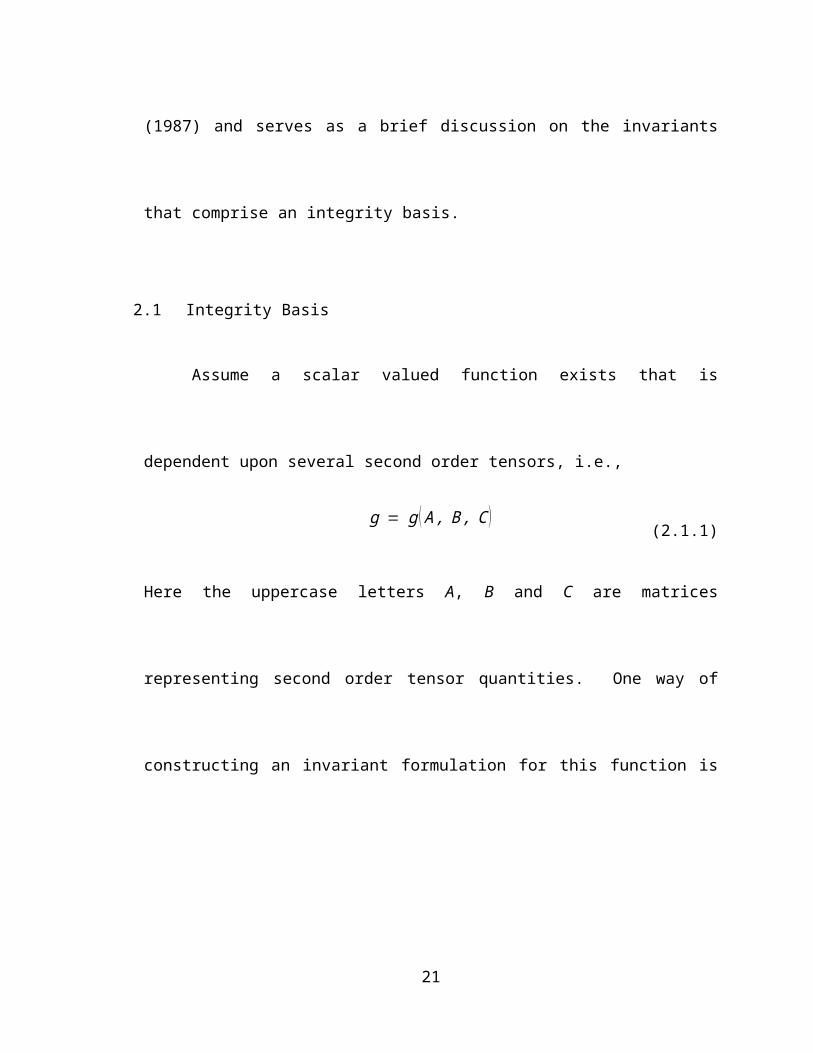
and the expression for f is form invariant. The invariants tr(A3), tr(A2), tr(A) constitute

the integrity basis for the function f. In general the results hold for the dependence on

any number of tensors. If the second order tensor represented by A is the Cauchy stress

tensor, then this infers the first three invariants of the Cauchy stress tensor span the

functional space for scalar functions dependent onij.

12

2.2 Useful Invariants of the Cauchy and Deviatoric Stress Tensors

If one accepts the premise from the previous section for a single second order

tensor, and if this tensor is the Cauchy stress tensor ij, then

g(σ ij) = g ( I 1 , I 2 , I 3)(2.2.1)

where

I 1 = σ ii (2.2.2)

I 2 = (12 ) ( (σ ii )2 − σ jk σ kj )

(2.2.3)

and

I 3 = ( 16 ) [ (2 ) (σ ij σ jk σ ki ) − (3 ) (σ ii ) (σ jk σ kj ) + ( σ ii )3 ]

(2.2.4)

are the first three invariants of the Cauchy stress. Since the invariants are functions of

principle stresses

I 1 = σ1 + σ 2 + σ 3 (2.2.5)

I 2 = σ1 σ 2 + σ 2 σ3 + σ1 σ3 (2.2.6)

and

I 3 = σ1 σ 2 σ3 (2.2.7)

then

13

g (σ ij ) = g ( I 1 , I 2 , I 3)¿ g (σ1 , σ2 , σ3 )

(2.2.8)

Furthermore, the stress tensor ij can be decomposed into a hydrostatic stress component

and a deviatoric component in the following manner. Take

Sij = σ ij − ( 13 )σ kk δij

(2.2.9)

If we look for the eigenvalues for the second order deviatoric stress tensor (Sij) using the

following determinant

|Sij − Sδij| = 0(2.2.10)

then the resultant characteristic polynomial is

S3 − J 1S2 − J 2 S − J3 = 0(2.2.11)

The coefficients J1, J2 and J3 are the invariants of Sij and are defined as

J1 = S ii = 0(2.2.12)

J2 = (12 )S ij S ji

¿ (13 ) I12 − I2

(2.2.13)

and

14

N

1

2

3

O

d

),,( 321 P

rComponentDevatoric

ComponentcHydrostati

J3 = (13 ) Sij S jk Ski

¿ (227 ) I13 − (13 ) I 1 I 2 + I3

(2.2.14)

These deviatoric invariants will be utilized as needed in the discussions that follow.

Figure 2.3.1 Decomposition of stress in the Haigh-Westergaard (principal) stress space

2.3 Graphical Representation of Stress

In the Haigh-Westergaard stress space a given stress state (1, 2, 3) can be

graphically decomposed into hydrostatic and deviatoric components. This decomposition

is depicted graphically in Figure 2.3.1. Line d in figure 2.3.1 represents the hydrostatic

axis where 1 = 2 = 3 such that the line makes equal angles to the coordinate axes. We

define the planes normal to the hydrostatic stress line as deviatoric planes. As a special

15

case the deviatoric plane passing through the origin is called the plane, or the

principal deviatoric plane. Point P (1, 2 , 3) in this stress space represents an arbitrary

state of stress. The vector NP represents the deviatoric component of the arbitrary stress

state, and the vector ON represents the hydrostatic component. The unit vector e in the

direction of the hydrostatic stress line d is

e = 1√3

[ 1 1 1](2.2.15)

The length of ON, which is identified as , is

ξ = (OP ) e

= [σ1 σ2 σ3 ] 1√3

¿ [ 1¿ ] [ 1¿ ]¿¿

¿

¿

¿

(2.2.16)

The length of NP, which is identified as a radial distance (r) in a deviatoric plane, is

r = O P − O N

= [ σ1 σ2 σ3 ] − (I 1

√3 ) [1 1 1 ]

¿ [S1 S2 S3 ] (2.2.17)

From this we obtain

| r | = r2

¿ S12 + S

22 + S32

¿ 2J 2 (2.2.18)

16

such that

r = √2 J 2 (2.2.19)

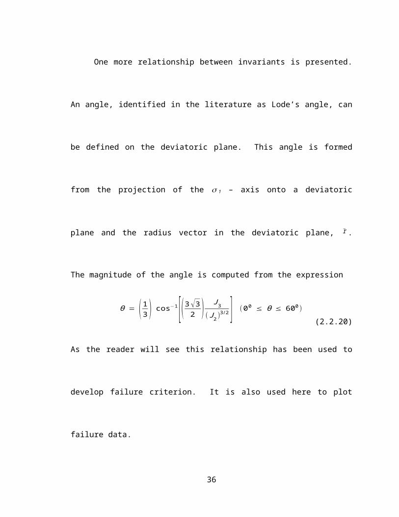
One more relationship between invariants is presented. An angle, identified in the

literature as Lode’s angle, can be defined on the deviatoric plane. This angle is formed

from the projection of the 1 – axis onto a deviatoric plane and the radius vector in the

deviatoric plane, r . The magnitude of the angle is computed from the expression

θ = ( 13 ) cos−1[( 3√3

2 ) J3

(J 2)3 /2 ] (00 ≤ θ ≤ 600 )

(2.2.20)

As the reader will see this relationship has been used to develop failure criterion. It is

also used here to plot failure data.

We now have several graphical schemes to present functions that are defined by

various failure criterions. They are

a principle stress plane (e.g., the 1 - 2 plane);

the use of a deviatoric plane presented in the Haigh-Westergaard stress

space; or

meridians along failure surfaces presented in the Haigh-Westergaard stress

space that are projected onto a plane defined by the coordinate axes (

ξ−r ).

17

Each presentation method will be utilized in turn to highlight aspects of the failure

criterion discussed herein. We begin with one parameter phenomenological models and

then discuss progressively more complex models.

2.4 Graphite Failure Data

In the following section several common failure criterion models will be

introduced and the constants for the models are characterized using biaxial failure data

generated by Burchell (2007). For the simpler models Burchell’s (2007) data has more

information than is necessary. For some models all the constants cannot be approximated

because there is not enough appropriate data for that particular model. These issues are

identified for each failure model. Burchell’s specimens were fabricated from grade H-

451 graphite. There were nine load cases presented, including two uniaxial tensile load

paths along two different material directions (data suggests that the material is

anisotropic), one uniaxial compression load path, and six biaxial stress load paths. The

test data is summarized in Table 2.1. The mean values of the normal stress components

for each load path from Burchell’s (2007) data are presented in Table 2.2. In addition,

corresponding invariants are calculated and presented in Table 2.2 along with Lode’s

angle. All the load paths (#B-1 through #B-9) are identified in Figure 2.4.1.

18

2.5 The von Mises Failure Criterion (One Parameter)

The von Mises criterion (1913) is based on failure defined by the octahedral

shearing stress reaching a critical value. Failure occurs along octahedral planes and the

basic formulation for the criterion is

19

Table 2.1 Grade H-451 Graphite: Load Paths and Corresponding Failure Data

Data Set

Ratio

Failure Stresses

(MPa）

# B-1 1 : 0

10.97 0

9.90 0

9.08 0

9.22 0

12.19 0

11.51 0

# B-2 0 : 1

0 15.87

0 12.83

0 18.06

0 20.29

0 14.32

0 14.22

# B-3 0 : - 1

0 -47.55

0 -50.63

0 -59.72

0 -56.22

0 -48.19

0 -51.54

# B-4 1 : - 19.01 -8.94

7.68 -7.68

14.34 -14.16

8.93 -8.78

13.23 -13.14

9.21 -9.11

Data Set

Ratio

Failure Stresses

(MPa）

# B-5 2 : 1

7.81 3.57

8.54 3.89

11.2 5.6

13.00 6.42

11.54 5.76

12.12 6.03

# B-6 1 : 2

6.36 12.67

6.42 12.86

6.74 13.42

7.69 15.36

6.46 12.95

7.17 14.36

# B-7 1 : - 2

7.98 -15.99

5.50 -10.96

6.69 -13.37

10.49 -21.01

9.18 -18.30

11.31 -22.61

Data Set

Ratio

Failure Stresses

(MPa）

# B-8 1 : 1.5

6.69 10.03

6.51 9.78

8.07 12.11

9.13 13.74

6.11 9.19

9.24 13.91

9.93 14.93

8.93 13.41

7.20 10.79

# B-9 1 : - 5 6.35 -31.61

8.69 -43.44

7.40 -36.86

20

7.09 -35.30

5.94 -29.50

6.83 -32.83

8.06 -40.21

7.75 -38.58

21

)(11 MPa

)(22 MPa

#B-2 #B-6#B-8

#B-5

#B-1

#B-4

#B-7

#B-9

#B-3

Figure 2.4.1 Burchell’s (2007) Load Paths Plotted in a 1 – 2 Stress SpaceTable 2.2 Invariants of the Average Failure Strengths for All 9 Load Paths

Data Set (1)ave (MPa) (2)ave (MPa) (MPa) r (MPa)

# B-1 10.48 0 6.05 8.56 0.00o

# B-2 0 15.93 9.20 13.01 0.00 o

# B-3 0 -52.93 -30.56 43.22 60.00 o

# B-4 10.4 -10.3 0.06 14.64 29.84 o

# B-5 10.7 5.21 9.19 7.57 29.13 o

# B-6 6.81 13.6 11.78 9.62 30.05o

# B-7 8.53 -17.04 -4.91 18.41 40.88 o

# B-8 7.98 11.99 11.53 8.63 40.82 o

# B-9 7.26 -36.04 -16.62 32.79 50.99 o

22

1x

2x

3x

T

T

g (σ ij ) = g ( J2 )¿ AJ2 − 1¿ 0 (2.5.1)

To determine the constant A consider the following stress state at failure

σ ij = ¿ [ 0 0 0 ¿ ] [0 σ T 0 ¿ ] ¿¿

¿(2.5.2)

here is the tensile strength of the material, and for this uniaxial load case

J2 = ( 13 )σ

T2

(2.5.3)

Substitution of the value of the invariant J2 into the failure function expressed in (2.5.1)

yields

A = 3σ

T2(2.5.4)

So the failure function for von Mises criterion takes the form

g (σ ij ) = ( 3σ

T2 )J2 − 1

(2.5.5)

As mentioned previously we have several means to graphically present the von

Mises criterion. The von Mises failure function is a right circular cylinder in the Haigh-

23

1

1I2

3

Westergaard stress space shown as Figure 2.5.1. The axis of the cylinder is coincident

with the hydrostatic stress line. The right circular cylinder is open along the hydrostatic

stress line (i.e., no end caps) in either the tensile or compressive direction. Thus a

hydrostatic state of stress cannot lead to failure.

Figure 2.5.1 von Mises failure in Haigh-Westergaard stress space

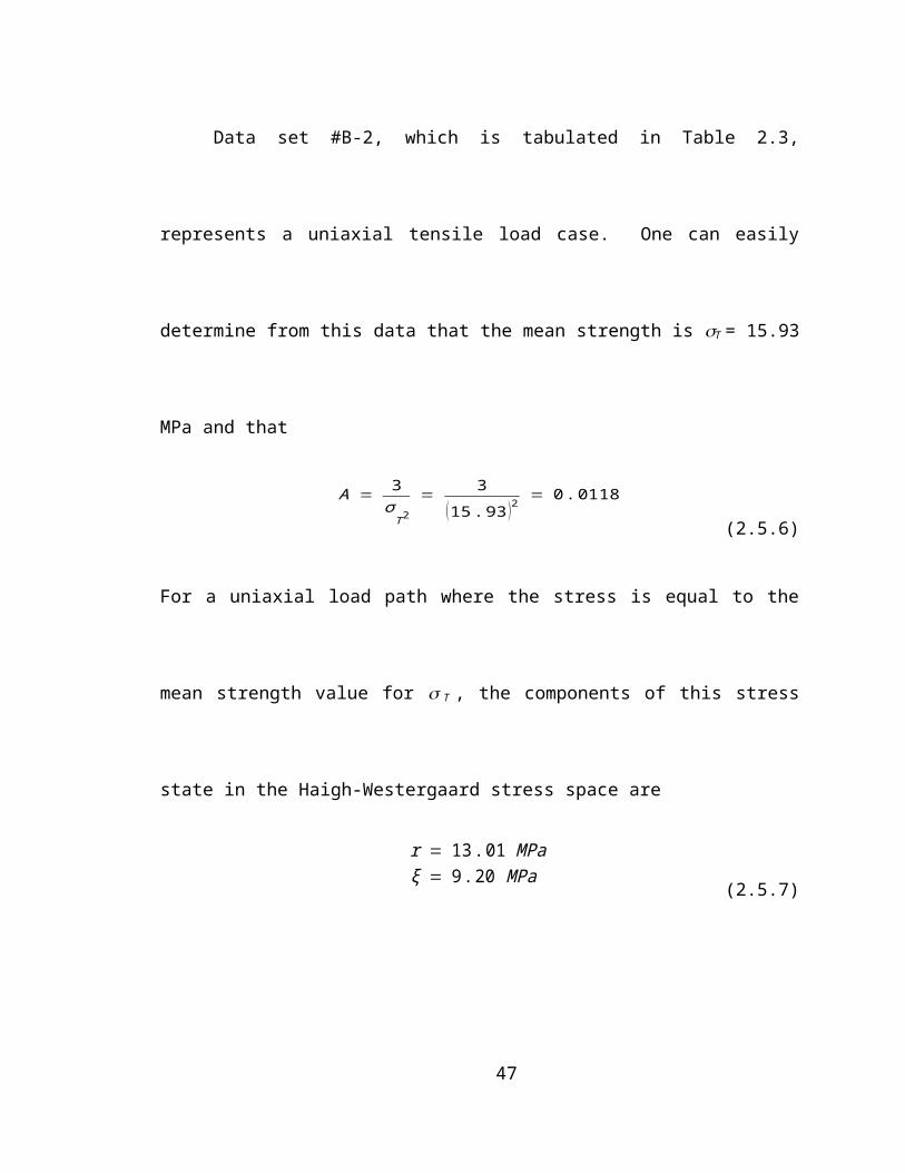
Data set #B-2, which is tabulated in Table 2.3, represents a uniaxial tensile load

case. One can easily determine from this data that the mean strength is T = 15.93 MPa

and that

A = 3σ

T2= 3

(15.93 )2= 0 .0118

(2.5.6)

For a uniaxial load path where the stress is equal to the mean strength value for T , the

components of this stress state in the Haigh-Westergaard stress space are

24

r = 13. 01 MPaξ = 9 .20 MPa

(2.5.7)

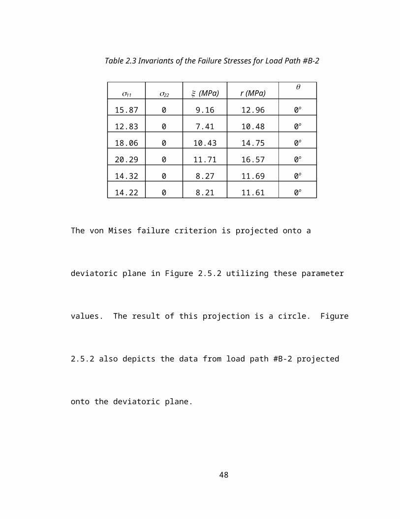
Table 2.3 Invariants of the Failure Stresses for Load Path #B-2

11

(MPa)

22

(MPa)

(MPa) r (MPa)

15.87 0 9.16 12.96 0o

12.83 0 7.41 10.48 0o

18.06 0 10.43 14.75 0o

20.29 0 11.71 16.57 0o

14.32 0 8.27 11.69 0o

14.22 0 8.21 11.61 0o

The von Mises failure criterion is projected onto a deviatoric plane in Figure 2.5.2

utilizing these parameter values. The result of this projection is a circle. Figure 2.5.2

also depicts the data from load path #B-2 projected onto the deviatoric plane.

25

3

11

2

3

o0

o60o120

o180

o240o330

)01.13,20.9(

,MPaMPa

r

MPa5

MPa15

MPa20

MPa10

2

Figure 2.5.2 The von Mises criterion is projected onto a deviatoric plane (ξ=9. 20 MPa ) parallel to the deviatoric plan with T = 15.93 MPa

The von Mises failure criterion is also projected onto a 1 - 2 stress plane in

Figure 2.5.3. A right circular cylinder projected onto this plane presents as an ellipse.

An aspect of the von Mises failure model is that tensile and compressive failure strengths

are equal which is clearly evident in Figure 2.5.3. Obviously the Burchell (2007) data,

which is also depicted in Figure 2.5.3, strongly suggests that tensile strength is not equal

to the compressive strength for this graphite material.

26

)(11 MPa

)(22 MPa

)93.15,0(, 2211 MPa

Figure 2.5.3 The Von Mises criterion characterized with (T = 15.93 MPa) projected onto the 1 -2 principle stress plane depicting failure stress values for all load paths

The third type of graphic presentation is a projection of the von Mises failure

criterion onto the coordinate plane identified by the axes (- r). As noted above the von

Mises criterion is a right circular cylinder in the principal stress space. The function

depicted in Figure 2.5.4 results from a cutting plane that contains the hydrostatic line

coinciding with the axis of the right circular cylinder. The axis of the cylinder is

coincident with the – axis and all meridians will be parallel to the – axis. Thus all

meridians along the surface of the right circular cylinder representing the von Mises

27

)(MPar

)(MPa

0

1322

Jf

Tij

MPaMPar 01.13,02.9,

failure criterion are identical, i.e., the slope of all meridians is zero and the intercepts

along the r-axis are the same value. This is not the case for subsequent failure criterion

presented below.

Figure 2.5.4 The Von Mises criterion projected onto a meridian plane (T = 15.93 MPa)

Using the average normal strength values for the nine data sets from Burchell

(2007) nine sets of invariants are tabulated in Table 2.2. This information is used to plot

the average strength data Figure 2.5.4. As can be seen in the figure most of the averaged

Burchell (2007) data does not match well with the von Mises criterion characterized with

28

T = 15.93 MPa. The depiction in Figure 2.5.4 strongly suggests that , or I1, should be

considered in developing the failure function, i.e., something more than the J2 should be

used to construct the model. Since nuclear graphite is not fully dense, we will assume

that the hydrostatic component of the stress state contributes to failure. In addition, the

von Mises criterion does not allow different strength in tension and compression. When

other formulations are considered in the next chapter their dependence will have a well-

defined dependence on I1. This invariant will permit different strengths in tension and

compression, e.g., the classic the Drucker–Prager (1952) failure criterion outlined in the

next section.

As a final note on the one parameter models, the Tresca (1865) could have been

considered here. However, Tresca’s (1865) criterion, although based on the concept that

failure occurs when a maximum shear strength of a material is attained, is a piecewise

continuous failure criterion. Although later criterion considered here are similarly

piecewise continuous, the Tresca (1865) failure criterion does not mandate continuous

gradients at the boundaries of various regions of the stress space. This condition will be

imposed on the failure criterion considered later.

29

CHAPTER III

TWO AND THREE PARAMETER FAILURE CRITERIA

In the previous chapter Burchell’s (2007) failure data was presented in terms of a

familiar one parameter failure criterion, i.e., the von Mises criterion. The von Mises

failure criterion can be characterized through a single strength parameter – the shear

strength on the octahedral stress plane. In this chapter the view is expanded and details

of two and three parameter failure criterion are presented in terms of how well the

criterion perform relative to the mean strength of various load directions from Burchell’s

work (2007).

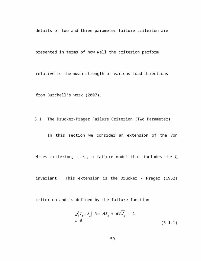
3.1 The Drucker-Prager Failure Criterion (Two Parameter)

In this section we consider an extension of the Von Mises criterion, i.e., a failure

model that includes the I1 invariant. This extension is the Drucker – Prager (1952)

criterion and is defined by the failure function

30

1x

2x

3x

T

T

g ( I 1 , J 2) = AI 1 + B √J2 − 1¿ 0 (3.1.1)

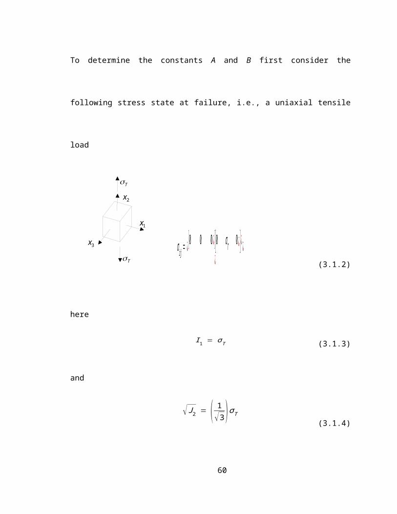
To determine the constants A and B first consider the following stress state at failure, i.e.,

a uniaxial tensile load

σ ij = ¿ [ 0 0 0 ¿ ] [0 σ T 0 ¿ ] ¿¿

¿(3.1.2)

here

I 1 = σT(3.1.3)

and

√J 2 = ( 1√3 )σT

(3.1.4)

Substitution of these invariants into the failure function (3.1.1) yields

A σ T + ( 1√3 ) BσT− 1 = 0

(3.1.5)

or

31

1x

2x

3x

C

C

A + ( 1√3 )B = 1

σT (3.1.6)

Next, consider the following stress state at failure under a uniaxial compression

load

σ ij=[0 0 00 −σ C 00 0 0 ]

(3.1.7)

where

I 1 = −σ C(3.1.8)

and

√J 2 = ( 1√3 )(σC )

(3.1.9)

Substitution of these invariants into the failure function (3.1.1) yields

A (−σC ) + ( 1√3 ) B σC − 1 = 0

(3.1.10)

or

32

−A + ( 1√3 ) B = 1

σ C (3.1.11)

Simultaneous solution of equations (3.1.6) and (3.1.11) yields

A = ( 12 ) ( 1

σ T−

1σC )

(3.1.12)

B = (√32 ) ( 1

σT+ 1

σC )(3.1.13)

Using the Burchell (2007) data from load path #B-2, the average tensile strength is

σ T = 15 . 93 MPa(3.1.14)

In a similar manner, using the load path #B-3, the average compressive strength is

σ C = 52. 93 MPa(3.1.15)

with these values of T and C the parameters A and B are

A = (12 ) (115 . 93− 1

52. 93 )= 0. 02194 MPa−1

(3.1.16)

and

B = (√32 ) (115 .93

+ 152.93 )

= 0.07073 MPa−1(3.1.17)

33

The Drucker-Prager (1952) failure criterion is projected onto the deviatoric plane

defined by

ξ = 9 . 20 MPa(3.1.18)

in Figure 3.1.1. There are an infinite number of deviatoric planes parallel to the -

plane. For the Drucker-Prager (1952) failure criterion each projection will represent a

circle with a different diameter on a different deviatoric plane. The graphical depiction

of the Drucker-Prager (1952) failure criterion on the deviatoric plane defined by

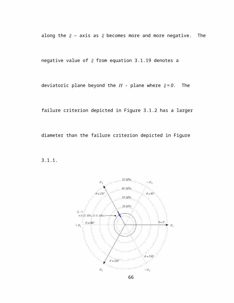
ξ = −30 .2 MPa(3.1.19)

also captures Burchell’s (2007) compressive data and is depicted in Figure 3.1.2. This

value of is obtained from averaging the compressive strength data along load path #B-

3. The invariants associated with the average strength from load path #B-3 are in Table

2.2. The invariants for all the failure strength data along load path #B-3 are presented in

Table 3.1. The Drucker-Prager (1952) failure criterion can be thought of as a right

circular cone with the tip of the cone located along the positive – axis. The cone opens

up along the – axis as becomes more and more negative. The negative value of

from equation 3.1.19 denotes a deviatoric plane beyond the - plane where = 0. The

failure criterion depicted in Figure 3.1.2 has a larger diameter than the failure criterion

depicted in Figure 3.1.1.

34

Figure 3.1.1 The Drucker-Prager (1952) criterion projected onto a deviatoric plane

(ξ=9. 20 Mpa) parallel to the -plane with T = 15.93 MPa, C =52.93 MPa

35

Figure 3.1.2 The Drucker-Prager (1952) criterion projected onto a deviatoric plane

(ξ=9. 20 Mpa) parallel to the -plane with T = 15.93 MPa, C = 52.93 MPa

Table 3.1 Invariants of the Failure Stresses for Load Path #B-3

11(MPa) 22(MPa) (MPa) r (MPa)

0 -47.55 -27.45 38.82 0o

0 -50.63 -29.23 41.34 0o

0 -59.72 -34.48 48.76 0o

0 -56.22 -32.46 45.90 0o

0 -48.19 -27.82 39.35 0o

0 -51.54 -29.76 42.08 0o

In Figure 3.1.3 the failure criterion is projected onto the 1 -2 stress plane and

compared with the entire data base from Burchell (2007). The right circular cone

typically projects as an elongated ellipse in this stress space. However, when the

Drucker-Prager (1952) failure criterion matches the mean failure stress along the 2 -

tensile load path (load path #B-2) and the 2 – compressive load path (load path #B-3) the

1 -2 stress plane slices through the right circular cone and produces a parabolic curve.

Note that the criterion does not match the Burchell (2007) data along the 2 tensile load

path (load path #B-1). The H-451 graphite Burchell (2007) tested is slightly anisotropic.

Moreover, the failure data from the biaxial stress load paths, #B-4 through #B-8 (the

36

exception is load path #B-9), are not captured at all since the failure curve is parabolic

and open along the equal biaxial compression load path. Anisotropic behavior and

parabolic failure curves (instead of elliptical curves) indicate a need for improvements

beyond the capabilities of the Drucker-Prager model in order to phenomenologically

capture the biaxial failure data.

37

)(11 MPa

)(22 MPa

)93.15,0(, 2211 MPa

)93.52,0(, 2211 MPa

Figure 3.1.3 The Drucker-Prager (1952) criterion projected onto the 1 -2 principle

stress plane (T = 15.93 MPa, C = 52.93 MPa)

The need for more flexibility is also evident when the Drucker-Prager (1952)

failure criterion is projected onto the stress space defined by the - r coordinate axes.

This projection is shown in Fig. 3.1.4 along with projections of the average strength

values from all nine load paths. As in the von Mises (1913) failure criterion, there is a

38

single meridian. The meridian for the Drucker-Prager (1952) failure criterion has a slope,

where the meridian for the von Mises (1913) failure criterion was parallel to the - axis.

As can be seen in Figure 3.1.4 three out of the nine average strength values align well

with the failure meridian projected into this figure based on the parameter values T =

15.93 MPa, and C = -52.93 MPa. These two parameters define the slope of the

meridian, and the meridian passes through the corresponding - r values, as it should.

The other six average strength values do not map closely to this single meridian for the

Drucker-Prager (1952) criterion. Keep in mind that the projection in Figure 3.1.4 is a

result of a cutting plane through the right circular cone and contains the hydrostatic stress

line. The data indicates that the failure function meridians should exhibit a dependence

on - defined by equation 2.2.20 and depicted in Figure 2.4.2. This can be accomplished

by including a dependence on the J3 invariant, and this is discussed in the next section.

39

)17.42,2.30(

,MPaMPa

r

)01.13,20.9(

,MPaMPa

r

)(MPar

)(MPa

Figure 3.1.4 The Drucker-Prager criterion projected onto the meridian plane(T = 15.93 MPa, C =52.93 MPa)

As noted above and depicted in Figure 3.1.3 the Drucker-Prager failure curve is

open along the equal biaxial compression load path. The following derivation will

demonstrate the transition from a parabolic (open) curve to an elliptic (closed) curve

based on the strength ratio C T. Consider the equal biaxial compression stress state

with BC < 0

σ ij = [−σBC 0 00 −σBC 00 0 0 ]

(3.1.20)

40

The corresponding deviatoric stress tensor is

Sij = [−σ BC

30 0

0 −σ BC

30

0 02σ BC

3]

(3.1.21)

The stress invariants of this state of stress are

I 1 = −2σ BC (3.1.22)

and

√J 2 = ( 1√3 )σ BC

(3.1.23)

Substitution of these invariants into the failure function (3.1.1) yields

A(−2σ BC) + B ( 1√3 ) σ BC− 1 = 0

(3.1.24)

or

σ BC = 1

−2 A + ( 1√3 ) B

(3.1.25)

Since BC > 0, then

σ BC = 1

−2 A + ( 1√3 ) B

> 0

(3.1.26)

41

which infers

2 A < ( 1√3 )B

(3.1.27)

This leads to

2( 12 ) ( 1

σ T− 1

σC ) < ( 1√3 )(√3

2 ) ( 1σT

+ 1σ C )

(3.1.28)

or

1σT

< 3σC

(3.1.29)

Thus

σC

σT< 3

(3.1.30)

When the ratio of compressive strength and tensile strength (C T) < 3, the Drucker-

Prager failure criterion projects an elliptical (closed) curve in the 1 -2 stress plane.

Consider the following biaxial state of stress

σ ij = [σ x 0 00 σ y 00 0 0 ]

(3.1.31)

The corresponding deviatoric stress tensor is

42

Sij = [2σ x−σ y

30 0

02 σ y−σ x

30

0 0 −σ x+σ y

3]

(3.1.33)

The stress invariants for this state of stress are

I 1 = σ x + σ y(3.1.32)

and

√J 2 = √( 13 )( σ

x2−σ x σ y+σy2)

(3.1.34)

Substitution of these invariants into equation (3.1.1) yields

f ( I 1 , J2 ) = A (σ x + σ y )

+ B√(13 ) (σ x2 − σ x σ y + σy2 ) − 1

¿ 0 (3.1.35)

or

√( 13 ) (σ x2 − σ x σ y + σ

y2 ) =1 − A (σ x + σ y )

B(3.1.36)

Squaring both sides yields

( B2−3 A )σx2 + (B2−3 A )σ y + (6 A−B2 )σ x σ

y2

+ 6 Aσ x + 6 Aσ y − 3 = 0 (3.1.37)

43

The shape of the failure criterion defined by equation (3.1.37) is determined by the values

of the two parameters A and B. Using Burchell’s (2007) tensile data where T = 15.93

MPa and a ratio of compressive strength to tensile strength of (C T) = 2, then C =-

31.86 MPa and the parameters A and B are

A = (12 ) (115 . 93− 1

31.86 )= 0. 01569 MPa−1

(3.1.38)

and

B = (√32 ) (115 . 93

+ 131 .86 )

= 0.08155 MPa−1(3.1.39 )

Equation (3.1.37) becomes

(0 . 0059 ) σx2 + ( 0. 0059 ) σ

y2 − (0 .0081 ) σ x σ y

+ (0 .0942 ) σx + (0. 0942 ) σ y = 3 (3.1.40 )

This expression is plotted in the 11 – 22 stress plane depicted in Figure 3.1.5

44

)(22 MPa

)(11 MPa

T 2,0, 2211

0,93.15, 2211 MPa

Figure 3.1.5 The Drucker-Prager (1952) criterion projected onto the 1 -2 principle

stress plane (T = 15.93 MPa, C = 31.86 MPa) and compared with the Burchell’s data

This combination of strength parameters leads to a biaxial strength of well over 900 MPa.

If Burchell’s (2007) compressive strength of C = 52.93 MPa is utilized from

along with a stress ratio (C T = 2), then the tensile strength is T =26.465 MPa. The

parameters A and B are

45

A = (12 ) (126 . 465− 1

52 . 93 )= 0. 009446 MPa−1

(3.1.41)

and

B = (√32 ) (126 . 465

+ 152 . 93 )

= 0.0490855 MPa−1(3.1.42)

Now

(0 .0021 ) σx2 + (0 . 0021 ) σ

y2 − (0.0029 ) σ x σ y

+ (0 .0567 ) σ x + (0 .0567 ) σ y = 3 (3.1.44)

This expression is plotted in the 11 – 22 stress plane depicted in Figure 3.1.6

NEED A THIRD FIGURE, 3.1.7 WHERE A NUMBER OF ELLIPSES ARE

SUPERIMPOSED IN THE SAME FIGURE. EACH ELLIPSE WOULD HAVE A

DIFFERENT STRENGTH RATIO OF C T RANGING FROM 1.0 TO 3.0 IN

INCREMENTS OF 0.25 OR 0.50.

46

47

MPa93.52,0, 2211

)(22 MPa

)(11 MPa

0,2/, 2211 C

Figure 3.1.6 The Drucker-Prager (1952) criterion projected onto the 1 -2 principle

stress plane (T = 18.25 MPa, C = -52.93 MPa) and compared with the Burchell’s data

Here the biaxial compressive strength is somewhat less than 1,100 MPa. In both figures,

i.e., Figure 3.1.5 and 3.1.6, closed ellipses are obtained which are important since all load

paths in this stress space eventually lead to failure. In Figure 3.1.3 the equal biaxial

compression load path was not bounded by the failure criterion given the strength

parameters from Burchell’s data. For all failure criterion considered, only those with

closed failure surfaces are relevant for consideration.

48

3.2 Willam-Warnke Failure Criterion (Three Parameter)

Willam and Warnke (1975) proposed a three-parameters failure criterion that

takes the shape of a pyramid with a triangular base in the Haigh-Westergaard (1 - 2 -

3) stress space. In a manner similar to the Drucker-Prager (1952) failure criterion, linear

meridians are assumed. However, the slopes of the meridians vary around the pyramidal

failure surface. The model is linear in stress through the use of I1 and √J 2 , which is

evident in the following expression

g ( I 1 , J 2 , J 3) = AI 1 + [ B(J 2 , J 3)] √J2 − 1¿ 0 (3.2.1)

Given the formulation above, in the Haigh-Westergaard stress space the Willam-

Warnke (1975) failure criterion is piecewise continuous with a threefold symmetry. This

symmetry is depicted in Figure 3.2.1 where the criterion is projected onto an arbitrary

deviatoric plane. The segment associated with 0o ≤ θ ≤ 60o

is presented. The

failure function is symmetric with respect to each tensile and compressive principle stress

axis projected onto the plane.

49

Figure 3.2.1 The Willam-Warnke (1975) criterion projected onto the deviatoric plane (

0o ≤ θ ≤ 60o)

As the deviatoric plane of the projection moves up the hydrostatic stress line in

the positive direction, the projection of the failure criterion shrinks. As the deviatoric

plane of projection moves down the hydrostatic line in the negative direction, the

projection of the failure criterion increases in size.

Willam and Warnke (1975) defined the parameter B from equation 3.2.1 in the

following manner

B = 1r (θ)

(3.2.2)

where r is a radial vector located in a plane parallel to the -plane. Willam and Warnke

(1975) assumed that when the failure surface was projected onto a deviatoric plane that a

50

1x

2x

3x

C

C

segment of this projection could be defined as a segment of an elliptic curve with the

following formulation

r (θ ) =2 rc(r

c2 − rt2)cosθ + r c(2 r t − rc )[ 4 ((r

c2 − rt2

)cos2 θ + 5 rt2 − 4 rt r c ]

1/2

4 ((rc2 − r

t2)cos2θ + (rc − 2 rt )2

(3.2.3)

Here is Lode’s angle, where once again

θ = ( 13 ) cos−1[( 3√3

2 ) (J 3)3

(J 2)3 ] (00 ≤ θ ≤ 600 )

(3.2.4)

When θ=0o, B=BT , r=rT and

rT = 1BT

(3.2.5)

Similarly, with θ=60o, B=BC , r=rC and

rC = 1BC

(3.2.6)

In order to determine the constants BT and BC consider the following stress state

σ ij = ¿ [ 0 0 0 ¿ ] [0 σ T 0 ¿ ] ¿¿

¿(3.2.7)

51

1x

2x

C

The deviatoric stress tensor is

Sij = ¿[− 13

0 0 ¿ ][ 0 23

0 ¿ ]¿¿

¿

(3.2.8)

and Lode’s angle as wells as the three invariants obtained are expressed as

( I1 , √J 2 , 3√J 3) = (σT , √33

σT ,3√23

σ T)(3.2.9)

θ = 00 (00 ≤ θ ≤ 600 )(3.2.10)

Substitution of the values of invariants into failure function given by equation (3.2.1)

yields

A( σT ) + (√33

BT )(σ T ) − 1 = 0(3.2.11)

or

A + ( √33 )BT = 1

σ T (3.2.12)

Next consider a uniaxial compressive stress state characterized by the following

stress tensor.

52

σ ij=[0 0 00 −σ C 00 0 0 ]

(3.2.13)

then

Sij = ¿[ 13

0 0 ¿][ 0 - 23

0 ¿]¿¿

¿

(3.2.14)

and

( I1 , √J 2 , 3√J 3) = (−σC , √33

σC ,3√23

σC )(3.2.15)

θ = 600

(3.2.16)

Substitution of these the values for the invariants into the Willam-Warnke (1975) failure

function yields

A(−σ C ) + (√33

BC)(σ C ) − 1 = 0(3.2.17)

−A + (√33 )BC = 1

σC (3.2.18)

53

1x

2x

3x

BC

BC

BCBC

At this point we have two equations (3.2.12 and 3.2.18) and three unknowns (A,

BT, and BC). In order to obtain a third equation consider an equal biaxial compressive

stress state characterized as

σ ij=[0 0 00 −σ BC 00 0 −σBC

](3.2.19)

Now the deviatoric stress tensor becomes

Sij = ¿[ 23

0 0 ¿] [ 0 - 13

0 ¿]¿¿

¿

(3.2.20)

and

( I1 , √J 2 , 3√J 3) = (−2 σBC , √33

σBC , −3√23

σBC)(3.2.21)

θ = 0o

(3.2.22)

Substitution of these invariants into failure function defined by equation (3.2.1) yields

(2 A ) (−σ BC) + (√33

BT ) (σ BC) − 1 = 0(3.2.23)

54

or

−2 A + (√33 )BT = 1

σBC (3.2.24)

We now have three equations, i.e., (3.2.12), (3.2.18) and (3.2.24), in three

unknowns A, Bt and Bc. Solution of this system of equations leads to the following three

expressions for the unknowns model parameters

A = ( 13 )( 1

σ T−

1σ C )

(3.2.25)

and

BT = (√33 )( 2

σT+ 1

σ BC )(3.2.26)

and

BC = (√3 ) [ 1σC

+ ( 13 )( 1

σT− 1

σ BC )](3.2.27)

In order to characterize to characterize the Willam and Warnke (1975) model in a

straight forward manner one would need failure data from a uniaxial load path, a uniaxial

compressive load path, and an equal biaxial compression load path. Unfortunately,

Burchell (2007) did not conduct biaxial compression stress tests. It must be pointed out

that these tests are extremely difficult to perform. Here we arbitrarily assume the

55

magnitude of the biaxial compression stress at failure is 1.16 times the uniaxial

compression stress at failure. Thus the three sets of strength parameters obtained from

the Burchell (2007) data are

T = 15.93 MPa (3.2.28)

for tension,

C = 52.93 MPa (3.2.29)

for compression and

BC = 61.40 MPa (3.2.30)

for the biaxial compression material strength. The important thing is that with the three

parameter Willam-Warnke (1975) criterion the biaxial compression strength is a direct

model input. Biaxial compression strength could be controlled indirectly in the Drucker-

Prager model (1952). The additional strength parameter in the Willam-Warnke (1975)

model brings additional flexibility and the criterion represents an increased flexibility in

modeling material behavior relative to the Drucker-Prager (1952) criterion in a manner

similar to a comparison of the Drucker-Prager (1952) model to the von Mises model

(1913). However, the additional flexibility is not enough to capture the anisotropic

behavior exhibited by Burchell’s (2007) graphite data.

This is evident in Figure 3.2.2 where the Willam-Warnke (1975) criterion and all

of Burchell’s (2007) test data are projected onto the principal stress plane defined by the

1 - 2 coordinate axes. The criterion seems to capture the biaxial failure data along load

56

path #B-8. However, there is an increasing loss of fidelity with load paths #B-7 and #B-

6. Load path #B-5 represents anisotropic strength behavior and the Willam and Warnke

(1975) model was constructed based on the assumption of an isotropic material. The

same behavior can be seen in biaxial load paths #B-4, #B-3 and #B-2. As we move away

from the load paths used to characterize the model parameters we encounter the loss in

fidelity and here we attribute the loss to material anisotropy. This anisotropic phenomena

will drive the research proposed for this effort.

IDENTIFY THE LOAD PATHS IN FIGURE 3.2.2 JUST LIKE FIGURE 2.4.1

57

MPa93.15,0

, 2211

MPaMPa 40.61,40.61

, 2211

MPa93.52,0

, 2211

1

1

)(11 MPa

)(22 MPa

Figure 3.2.2 The Willam-Warnke(1975) criterion projected onto the 1 -2 principle stress plane (T = 15.93 MPa, C = 52.93 MPa, BC = 61.40 MPa)

Varying the biaxial compressive strength of the material does not help in

matching the criterion with the data from biaxial load paths #B-2 through #B-4 and load

paths #B-6 as well as #B-7. This is evident in Figure 3.2.3 where the biaxial strength is

varied from 0.96 of the uniaxial compression strength to 1.16 times the uniaxial

58

)(11 MPa

)(22 MPa

compressive strength. The various projections based on differing values of BC did not

improve the criterion’s ability to match the data from the load paths just mentioned.

Figure 3.2.3 The Willam-Warnke(1975) criterion projected onto the 1 -2 principle stress plane for multiple T = 15.93 MPa, C = 52.93 MPa, and BC = 56.11MPa, 61.40

MPa, 66.69Mpa

In Figures 3.2.4 and 3.2.5 the Willam-Warnke (1975) model is projected onto

deviatoric planes. In Figure 3.2.4

ξ = 9 . 20 MPa (3.2.31)

and in Figure 3.2.5

59

ξ = −30 .2 MPa(3.2.32)

In these figures the Willam-Warnke (1975) criterion presents as slices through a right

triangular pyramid.

Figure 3.2.4 The Willam-Warnke criterion projected onto a deviatoric plane

(ξ=6 . 05 Mpa) parallel to the -plane with T = 15.93 MPa, C = 52.93 MPa,

BC = 61.40 MPa

60

)(MPa

)(MPar

o30

o60

o0

)0,13.50,9.70(),,( oBC MPaMPar

)60,33.43,56.30(),,( oC MPaMPar

)0,01.13,02.9(),,( oT MPaMPar

Figure 3.2.5 The Willam-Warnke criterion projected onto a deviatoric plane

(ξ1=−30 . 2 MPa) parallel to the -plane with T = 15.93 MPa, C = 52.93 MPa,

BC =61.40 MPa

Figure 3.2.6 The Willam-Warnke criterion projected onto the meridian plane for a material strength parameter of T = 15.93 MPa, C = 52.93 MPa,

BC = 61.40 MPa

The meridian lines associated with the Willam-Warnke (1975) failure criterion for

Lode angle values of θ=0oandθ=60o

are depicted on Figure 3.2.6. The meridians for

each Lode angle are distinct from one another since one is a tensile meridian and passes

through the tensile strength parameter along a principle stress axis. The other is a

61

compressive meridian and intercepts a principle stress axis at the value of the

compressive strength parameter. The θ=0omeridian line goes through point (r = 9.02

MPa, = 13.01 MPa) and the θ=60omeridian line goes through point (r = 30.56 MPa,

= 43.22 MPa) as they should since these data values were used to characterize the

model. The point (r = 6.05 MPa, = 8.56 MPa) represents the average strength for load

path #B-5, a uniaxial load path that was not used to characterize the model. The data

from load path #B-5 represents anisotropic strength behavior and one should not expect

this data to match well with the isotropic Willam-Warnke (1975) model.

Up to this point it has been noted several times that Burchell’s data (2007)

exhibits anisotropic behavior. As part of this effort many attempts were made to extend

the Willam-Warnke (1975) model in order to capture anisotropic behavior through the

use of tensor based stress invariants. The primary difficulty with extending the Willam-

Warnke (1975) failure criterion to anisotropy is the fact that the function is linear in stress

and based on a trial and error approach, the belief here is that at least a quadratic

dependence is needed in order to capture anisotropic behavior through stress invariants.

The next section presents a failure criterion analogous to the Willam-Warnke (1975)

failure model that is quadratic in stress.

62

CHAPTER IV

ISOTROPIC GREEN-MKRTICHIAN FAILURE CRITERION

The next phenomenological failure criterion considered in this effort was

proposed by Green and Mkrtichian (1977) and has the basic form

g = g (σ ij , a i )(4.1)

Green and Mkrtichian (1977) track the principle stress direction vectors, identified here

as ai. Utilizing the eigenvectors of the principal stresses enables the identification of

tensile and compressive principle stress directions. The authors of this model consider

different behavior in tension and compression as a type of material anisotropy. Utilizing

first order tensors (the eigenvectors) as directional tensors is an accepted approach in

modeling anisotropy through the use of invariants. Spencer (1984) pointed out the

mathematics that underlies the concept. This model produces results very similar to the

Willam-Warnke (1975) failure criterion. The utility of the isotropic form of the Green-

Mkrtichian (1977) model is that this failure criterion is quadratic in stress whereas the

63

Willam-Warnke (1975) failure criterion was linear in stress. Being quadratic in stress

makes the Willam-Warnke (1975) model more amenable to including anisotropic

behavior, which is discussed in the next chapter. This chapter outlines fundamental

aspects of the Willam-Warnke (1975) failure criterion in preparation for the extension to

anisotropy.

4.1 Integrity Basis and Functional Dependence

The integrity basis for the a function with a dependence specified in equation

(4.1) is

iiI 1(4.1.1)

I 2 = σ ij σ ji (4.1.2)

I 3 = σ ij σ jk σki (4.1.3)

I 4 = ai a j σ ij (4.1.4)

and

I 5 = ai a j σ jk σki (4.1.5)

These invariants (with the exception of I3, which can be derived from I1 and I2) constitute

an integrity basis and span the space of possible stress invariants that can be utilized to

64

compose scalar valued functions that are dependent on stress. Thus the dependence of

the Green and Mkrtichian (1977) failure criterion can be characterized in general as

g (σ ij ) = g ( I 1 , I 2 , I 4 , I 5)(4.1.6)

One possible polynomial formulation for g in terms of the integrity basis is

g (σ ij ) = A ( I1 )2 + B I 2 + C I 1 I 4 + D I 5 − 1(4.1.7)

This functional form is quadratic in stress which, as is seen in the next section, is

convenient when extending this formulation to include anisotropy. The invariants I4 and

I5 are associated with the directional tensor ai, and we note that Green and Mkrtichian

(1977) utilized these invariants in the functional dependence very judiciously. They

partitioned the Haigh-Westergaard stress space and offered four forms for the failure

functions.

4.2 Functional Forms and Associated Gradients by Stress Region

By definition the principal stresses are identified such that

σ 1 ≥ σ 2 ≥ σ3(4.2.1)

The four functions proposed by Green and Mkrtichian (1977) span the stress space which

is partitioned as follows:

Region #1: σ 1 ≥ σ 2 ≥ σ3 ≥ 0 – all principal stresses are tensile

65

Region #2: σ 1 ≥ σ 2 ≥ 0 ≥ σ3 – one principal stress is compressive, the

others are tensile

Region #3: σ 1 ≥ 0 ≥σ2 ≥ σ3 – one principal stress is tensile, the others are

compressive

Region #4: 0 ≥ σ1 ≥ σ2 ≥ σ3 – all principal stresses are compressive.

Thus the Green and Mkrtichian (1977) criterion has a specific formulation for the case of

all tensile principle stresses, and a different formulation for all compressive principle

stresses (see derivation below). For these two formulations there is no need to track

principle stress orientations and thus for Regions #1 and #4 the Green and Mkrtichian

(1977) failure criterion did not include the terms associated with I4 and I5, both of which

contain information regarding the directional tensor. A third and fourth formulation

exists for Regions #3 and #4 where two principle stresses are tensile and when two

principle stresses are compressive, respectively and the failure behavior depends on the

direction of the principal tensile and compressive stresses. For these regions of the stress

space for the Green and Mkrtichian (1977) failure criterion includes the invariants I4 and

I5.

The functional values of the four formulations g1, g2, g3 and g4 must match along

their common boundaries. In addition, the tangents associated with the failure surfaces

66

along the common boundaries must be single valued. This will provide a smooth

transition from one region to the next. To insure this, the gradients to the failure surfaces

along each boundary are equated. The specifics of equating the formulations and

equating the gradients at common boundaries are presented below. Relationships are

developed for the constants associated with each term of the failure function for the four

different regions.

Region #1: (σ1 ≥ σ2 ≥ σ3 ≥0 ) Green and Mkrtichian (1977) assumed

the failure function for this region of the stress space is

g1 = 1 − [( 12 ) A1 I

12 + B 1 I 2 ](4.2.2)

From equation (4.2.10) it is evident that there will be a group of constants for each region

of the stress space. Hence the subscripts for the constants associated with each invariant

as well as the failure function will run from one to four. Also note the absence of

invariants I4 and I5. The corresponding normal to the failure surface is

∂ g1

∂σ ij=

∂ g1

∂ I 1

∂ I 1

∂ σ ij+

∂ g1

∂ I 2

∂ I 2

∂ σ ij (4.2.3)

where

∂ g1

∂ I1= −A1 I 1

(4.2.4)

67

∂ g1

∂ I2= −B1

(4.2.5)

∂ I 1

∂σ ij= δij

(4.2.6)

and

∂ I 2

∂σ ij= 2 σ ij

(4.2.7)

Here ij is the Kronecker delta tensor. Substitution of equations (4.2.4) through (4.2.7)

into (4.2.3) leads to the following tensor expression

∂ g1

∂σ ij= −( A1 I 1 δij + 2 B1 σ ij )

(4.2.8)

or in a matrix format

∂ g1

∂ σ ij= [σ1+σ2+σ 3 0 0

0 σ 1+σ 2+σ 3 00 0 σ1+σ2+σ3

] (−A1)

+ [2 σ1 0 00 2σ2 00 0 2σ3

] (−B1 )

(4.2.9)

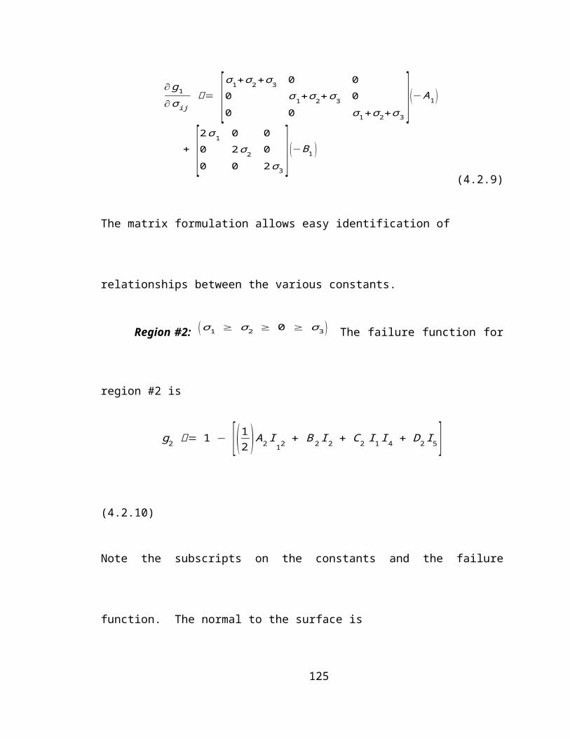
The matrix formulation allows easy identification of relationships between the various

constants.

Region #2: (σ1 ≥ σ2 ≥ 0 ≥ σ 3) The failure function for region #2 is

68

g2 = 1 − [( 12 ) A2 I

12 + B 2 I2 + C2 I 1 I 4 + D2 I 5 ] (4.2.10)

Note the subscripts on the constants and the failure function. The normal to the surface is

∂ g2

∂σ ij=

∂ g2

∂ I 1

∂ I 1

∂ σ ij+

∂ g2

∂ I2

∂ I 2

∂σ ij+

∂ g2

∂ I 4

∂ I 4

∂ σ ij+

∂ g2

∂ I 5

∂ I5

∂ σ ij (4.2.11)

Here

∂ g2

∂ I1= −( A2 I 1 + C2 I 4 )

(4.2.12)

∂ g2

∂ I 2= −B2

(4.2.13)

∂ g2

∂ I 4= −C2 I 1

(4.2.14)

∂ g2

∂ I5= −D2

(4.2.15)

∂ I 4

∂σ ij= ai a j

(4.2.16)

and

∂ I 5

∂σ ij= ak a i σ jk + a j ak σ ki

(4.2.17)

69

The principle stress direction of interest in this region of the stress space is the one

associated with the third principal stress. Assuming the Cartesian coordinate system is

aligned with the principal stress directions then the eigenvector associated with the third

principal stress is

a i = (0 , 0 , 1 )(4.2.18)

Thus for equation (4.2.16) and (4.2.17)

ak a i = a j ak = ai a j = [001 ] [0 0 1 ]

¿ [0 0 00 0 00 0 1 ]

(4.2.19)

Given the principle stress direction of interest the fourth and fifth invariants are

I 4 = σ 3(4.2.20)

and

I 5 = σ32

(4.2.21)

for this region of the stress space. Substitution of equations (4.2.12) through (4.2.21) into

(4.2.11) yields the following tensor expression for the normal to the failure surface

∂ g2

∂ σ ij= −[ A2 I1 δij + 2B2 σ ij + C2( σ3 δ ij + I1 ai ai )

+ D2 (ak ai σ jk + a j ak σ ki) ] (4.2.22)

70

The matrix form of equation (4.2.22) is

∂ g2

∂ σ ij= [σ1+σ2+σ 3 0 0

0 σ 1+σ 2+σ 3 00 0 σ1+σ2+σ3

] (−A2) + [2 σ1 0 00 2σ 2 00 0 2σ3

] (−B2)

+ [σ 3 0 00 σ 3 00 0 σ 1+σ 2+2 σ3

] (−C2 ) + [0 0 00 0 00 0 2 σ3

] (−D2)

(4.2.23)

Region #3:(σ1 ≥ 0 ≥σ2 ≥ σ 3) The failure function for this region of the

stress space is

g3 = 1 − [(12 ) A3 I

12 + B 3 I 2 + C3 I1 I 4 + D3 I 5] (4.2.24)

The normal to the surface is

∂ g3

∂σ ij=

∂ g3

∂ I 1

∂ I 1

∂σ ij+

∂ g3

∂ I 2

∂ I 2

∂ σ ij+

∂ g3

∂ I 4

∂ I 4

∂ σ ij+

∂ g3

∂ I5

∂ I 5

∂σ ij (4.2.25)

Here

∂ g3

∂ I 1= −( A3 I1 + C3 I 4 )

(4.2.26)

∂ g3

∂ I 2= −B3

(4.2.27)

∂ g3

∂ I 4= −C3 I1

(4.2.28)

71

and

∂ g3

∂ I5= −D3

(4.2.29)

The principle stress direction of interest for this stress state is the one associated with the

first principal stress, i.e.,

a i = (1 , 0 , 0 )(4.2.30)

Now

ak a i = a j ak = ai a j = [100 ] [1 0 0 ]

¿ [1 0 00 0 00 0 0 ]

(4.2.31)

The fourth and fifth invariants for this region of the stress space are

I 4 = σ1(4.2.32)

and

I 5 = σ12

(4.2.33)

Substitution of the quantities specified above into (4.2.25) yields the following tensor

expression

72

∂ g3

∂ σ ij= −[ A3 I1 δij + 2 B3 σ ij + C3 (σ1 δ ij + I 1 ai a j )

+ D3( ak a i σ jk + a j ak σki )] (4.2.34)

The matrix form of this equation is as follows

∂ g3

∂ σ ij= [σ1+σ2+σ 3 0 0

0 σ 1+σ 2+σ 3 00 0 σ1+σ2+σ3

] (−A3 ) + [2 σ1 0 00 2σ 2 00 0 2σ3

] (−B3)

+ [2 σ1+σ2+σ3 0 00 σ1 00 0 σ1

] (−C3) + [2 σ1 0 00 0 00 0 0 ](−D3)

(4.2.35)

Region #4: 0 ≥ σ1 ≥ σ2 ≥ σ3 The failure function for this region of the

stress space is

g4 = 1 − [( 12 ) A4 I

12 + B 4 I2 ](4.2.36)

The corresponding normal to the failure surface is

∂ g4

∂σ ij=

∂ g4

∂ I 1

∂ I1

∂ σ ij+

∂ g4

∂ I2

∂ I 2

∂ σ ij (4.2.37)

Here

∂ g4

∂ I 1= A4 I 1

(4.2.38)

and

73

∂ g4

∂ I 2= B4

(4.2.39)

Substitution of the equations above into (4.2.37) yields the following tensor expression

∂ g4

∂σ ij= 1 − ( A4 I 1 δij + 2 B4 σ ij )

(4.2.40)

The matrix format of this expression is

∂ g4

∂ σ ij= [σ1+σ2+σ3 0 0

0 σ1+σ2+σ 3 00 0 σ 1+σ 2+σ 3

](− A4)

+ [2 σ1 0 00 2 σ2 00 0 2σ 3

](−B4 )

(4.2.41)

4.3 Relationships Between Functional Constants

With the failure functions and the normals to those functions defined for each

region, attention is now turned to defining the constants. Consider the region of the

Haigh-Westergaard stress space where with andThe stress

state in a matrix format is

σ ij = ¿ [σ1 0 0 ¿ ] [0 σ2 0 ¿ ]¿¿

¿(4.3.1)

74

and this stress state lies along the boundary shared by region #1 and region #2. At this

boundary we impose

g1 = g2 (4.3.2)

and

∂ g1

∂σ ij=

∂ g2

∂ σ ij (4.3.3)

For this stress state the invariants I1 and I2 are

I 1 = σ1 + σ 2(4.3.4)

and

I 2 = σ12 + σ

22

(4.3.5)

for both g1 and g2. The invariants I4 and I5 for g2 are

I 4 = σ 3 = 0(4.3.6)

and

I 5 = (σ3 )2 = 0(4.3.7)

Substitution of equations (4.3.4) through (4.3.7) into equation (4.3.1) yields the following

matrix expression

75

[σ1+σ2+σ3 0 00 σ1+σ2+σ3 00 0 σ1+σ 2+σ 3

]A1 + ¿ [2 σ1 0 0 ¿ ] [0 2 σ2 0 ¿ ] ¿¿

¿

¿

¿

(4.3.8)

with

σ 3 = 0(4.3.9)

then

[σ1+σ2 0 00 σ1+σ2 00 0 σ1+σ 2

] A1 + ¿ [2σ1 0 0¿ ] [ 0 2σ2 0¿ ]¿¿

¿

¿

¿

(4.3.10)

The following three expressions can be extracted from equation (4.3.10)

(σ1+σ2 ) A1 + (2 σ 1)B1 = (σ1+σ2 ) A2 + (2 σ1 )B2(4.3.11)

(σ1+σ2 ) A1 + (2 σ 2) B1 = (σ1+σ2 ) A2 + (2 σ 2)B2(4.3.12)

76

1x

2x

3x

2

23

3

(σ1+σ2 ) A1 = (σ1+σ2 ) A2 + (σ1+σ2 )C2(4.3.13)

The constant D2 does not appear due to its multiplication with the null matrix. However,

C2 does appear in the third expression but in the first two immediately above. Focusing

on equation (4.3.11) and equation (4.3.12) which represents two equations in two

unknowns then

B1 = B2(4.3.14)

and

A1 = A2(4.3.15)

Substitution of equation (4.3.15) into equation (4.3.13) yields

C2 = 0(4.3.16)

and at this point D2 is indeterminate. Substitution of equations (4.3.4) through (4.3.7)

into equation (4.3.2) yields the following expression

Now consider the region of the Haigh-Westergaard stress space where

and The stress state in a matrix format is

σ ij = ¿ [σ1 0 0 ¿ ] [ 0 0 0 ¿ ]¿¿

¿(4.3.17)

77

and this stress state lies at the boundary shared by region #2 and region #4. At this

boundary we impose

g2 = g3(4.3.18)

and

∂ g2

∂σ ij=

∂ g3

∂ σ ij (4.3.19)

Under these conditions the invariants I1 and I2 are

I 1 = σ1 + σ 3(4.3.20)

and

I 2 = σ12 + σ

32(4.3.21)

Substitution of equation (4.3.20) and (4.3.21) into equation (4.3.19) yields

¿ [ σ1+σ 2+σ 3 0 0¿ ] [ 0 σ1+σ2+σ3 0¿ ]¿¿

¿

¿¿

(4.3.22)

78

with

σ 2 = 0(4.3.23)

then

¿ [ σ1+σ 3 0 0 ¿ ] [ 0 σ1+σ3 0¿ ] ¿¿

¿

¿¿

(4.3.24)

The following three expressions can be extracted from equation (4.3.24)

(σ1+σ3 ) A2 + (2 σ1) B2 + ( σ3 )C2

¿ (σ1+σ3 ) A3 + (2 σ1) B3 + ( 2σ1+σ 3)C3 + (2 σ1 ) D3 (4.3.25)

(σ1+σ3 ) A2 + ( σ3 )C2 = ( σ1+σ 3 ) A3 + (σ 1) C3(4.3.26)

and

(σ1+σ3 ) A2 + (2σ3) B2 + (σ1+2σ 3) C2 + (2σ3 ) D2

¿ (σ1+σ3) A3 + (2 σ3) B3 + (σ1 ) C3 (4.3.27)

Earlier it was determined that C2 = 0, so from equation (4.3.26) we obtain

79

A2 = A3 +σ3

(σ1+σ3 )C3

(4.3.28)

From equation (4.3.74) and equation (4.3.75) we obtain

B2 = B3 +(σ1+σ3)

2 σ1C3 + D3

(4.3.29)

In addition, from equation (4.3.27) and equation (4.3.26) we obtain

D2 = −(σ1+σ3 )

2 σ1C3 − D3

(4.3.30)

Consider the Region of the Haigh-Westergaard stress space where

and The stress state in a matrix format is

σ ij = ¿ [ 0 0 0 ¿ ] [0 σ 2 0¿ ]¿¿

¿(4.3.31)

and this stress state lies along the boundary shared by region #3 and region #4. At this

boundary we impose

g3 = g4(4.3.32)

and

∂ g3

∂σ ij=

∂ g4

∂ σ ij (4.3.33)

Under these conditions the invariants I1 and I2 are

80

I 1 = σ2 + σ 3(4.3.34)

and

I 2 = σ22 + σ

32(4.3.35)

Substitution of equations (4.3.34) and (4.3.35) into equation (4.3.32) yields

[σ1+σ2+σ3 0 00 σ1+σ 2+σ 3 00 0 σ 1+σ 2+σ3

]A3 + [2 σ 1 0 00 2σ2 00 0 2 σ 3

]B3

+ [2 σ1+σ2+σ3 0 00 0 00 0 0 ]C3 + [2 σ1 0 0

0 0 00 0 0 ] D3

¿ [σ1+σ2+σ3 0 00 σ1+σ2+σ3 00 0 σ1+σ2+σ 3

] A4

+ [2σ 1 0 00 2σ2 00 0 2σ 3

]B4

(4.3.36)

with

σ 1 = 0(4.3.37)

then

81

¿ [ σ2+σ 3 0 0 ¿ ] [ 0 σ2+σ3 0 ¿ ] ¿¿

¿

¿¿

(4.3.38)

The following three expressions can be extracted from equation (4.3.38)

(σ 2+σ3 ) A3 + (σ2+σ3 ) C3 = (σ2+σ3 ) A4(4.3.39)

(σ 2+σ3 ) A3 + (2 σ2) B3 = ( σ2+σ3 ) A4 + (2 σ2) B4(4.3.40)

and

(σ 2+σ3 ) A3 + (2 σ3 )B3 = (σ2+σ3 ) A4 + (2 σ3 )B4(4.3.41)

From equation (4.3.39) we discern that

A3 + C3 = A4(4.3.42)

From equation (4.3.40) and equation (4.3.41) we obtain

(2 σ 2−2 σ 3) B3 = (2 σ2−2 σ3 )B4(4.3.43)

or that

82

B3 = B4(4.3.44)

Substitution of equations (4.2.34) and (4.2.35) into equation (4.3.41) leads to

A3 = A4(4.3.45)

and

C3 = 0(4.3.46)

Substitution of equation (4.3.46) into equations (4.3.28), (4.3.29) and (4.3.30) yields

A2 = A3(4.3.47)

B2 = B3 + D3(4.3.48)

and

D2 = − D3(4.3.49)

So the relationships between the functional constants is as follows

A1 = A2 = A3 = A4(4.3.50)

B1 = B2= B3 − D2= B4 − D2(4.3.51)

C2 = C3 = 0(4.3.52)

and

D2 + D3 = 0(4.3.53)

83

1x

2x

3x

T

T

These relationships insure that the four functional forms for the failure function are

smooth and continuous along the boundaries of the four regions.

4.4 Functional Constants in Terms of Strength Parameters

Next we utilize specific load paths in order to define the constants defined above

in terms of stress values obtained at failure. Consider the following stress state at failure

under a uniaxial tensile load

σ ij = [0 0 00 σT 00 0 0 ]

(4.4.1)

This stress state lies on the boundary of region #1. The invariants for this stress state are

I 1 = σT(4.4.2)

and

I 2 = σT2

(4.4.3)

The failure function takes the form

g1 = 1 − [12 A1 (σT )2 + B1 (σT )2 ]¿ 0

(4.4.4)

84

1x

2x

3x

C

C

from which the following relationship is obtained

12

A1 + B1 = 1σ

T2(4.4.5)

Next a uniaxial compressive stress state is considered where

σ ij = [0 0 00 0 00 0 σ C

](4.4.6)

The principle stress direction for this stress state is

a i = (0 , 0 , 1 )(4.4.7)

thus

a i a j = [0 0 00 0 00 0 1 ]

(4.4.8)

The invariants are as follows

I 1 = −σ C(4.4.9)

I 2 = (−σC )2(4.4.10)

85

1x

2x

3x

BC

BC

BCBC

I 4 = σC(4.4.11)

and

I 5 = (−σC )2(4.4.12)

Thus

g2 = 12

A2 ( σC )2 + B2 (σC )2 + D2 (σC )2 −1

¿ 0(4.4.13)

which leads to

12

A2 + B2 + D2 = 1σ

C2(4.4.14)

Next consider an equal biaxial compressive stress state where

σ ij = [0 0 00 −σ BC 00 0 −σ BC

](4.4.15)

86

This stress state lies within region #4 and the invariants are as follows

I 1 = −2 σ BC(4.4.16)

and

I 2 = σBC 2

(4.4.17)

The failure function for this particular stress state is

f 4 = 12

A4 (2σ BC )2 + B4 (2 σBC2) − 1

¿ 0(4.4.18)

which leads to

A1 + B1 + D2 = 12 (σ BC )2

(4.4.19)

Solving equations (4.4.5), (4.4.4) and (4.4.19) using equations (4.3.50) through (4.3.53)

leads to

A1 = A2 = A3 = A4 = 1σ

BC2− 2

σC2

(4.4.20)

B1 = B2 = 1σ

T2− 1

2 σBC2

+ 1σ

C2(4.4.21)

B3 = B4 = 2σ

C2− 1

2 σBC 2

(4.4.22)

and

87

D2 = −D3 = 1σ

C2− 1

σT2

(4.4.23)

In order to visualize the isotropic version of the Green and Mkrtichian (1977)

failure criterion relative to Burchell’s (2007) failure data, values were computed for the

strength constants immediately above, i.e., T = 15.93 MPa for tension, C = 52.93 MPa

for compression and BC = 61.40 MPa for the biaxial compression. The values for T and

C and were obtained directly from Burchell’s (2007) data. The value for BC was

determined by a best fit approximation of the failure curve to the data in Figure 4.4.1.

Various projections of the isotropic Green and Mkrtichian (1977) failure criterion are

presented in the next several figures along with the Burchell (2007) data. The first is a

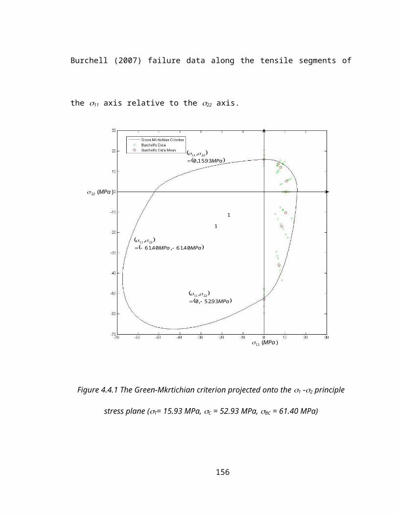
projection onto the 11 – 22 stress space which is depicted in Figure 4.4.1. As can be

seen in this figure the isotropic Green and Mkrtichian (1977) model captures the different

behavior in tension and compression exhibited by the Burchell (2007) data along the 22

axis. However, the Green and Mkrtichian (1977) failure criterion does not capture

material anisotropy which is clearly exhibited by the Burchell (2007) failure data along

the tensile segments of the 11 axis relative to the 22 axis.

88

MPa93.15,0

, 2211

MPaMPa 40.61,40.61

, 2211

MPa93.52,0

, 2211

1

1

)(11 MPa

)(22 MPa

Figure 4.4.1 The Green-Mkrtichian criterion projected onto the 1 -2 principle stress plane (T= 15.93 MPa, C = 52.93 MPa, BC = 61.40 MPa)

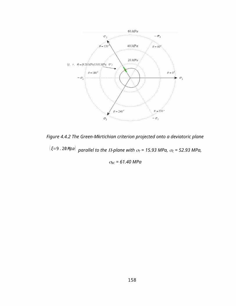
The isotropic Green and Mkrtichian (1977) failure criterion is projected onto the

deviatoric planes in Figures 4.4.2 and 4.4.3. Note that a cross section through the failure

function perpendicular to the hydrostatic axis transitions from a pyramidal shape (Figure

4.4.3) to a circular shape (Figure 4.4.2) with an increasing value of the stress invariant I1.

This suggests that the apex of the failure function presented in a full Haigh-Westergaard

stress space is blunt, i.e., quite rounded for the this particular criterion.

89

Figure 4.4.2 The Green-Mkrtichian criterion projected onto a deviatoric plane

(ξ=9. 20 Mpa) parallel to the -plane with T = 15.93 MPa, C = 52.93 MPa,

BC = 61.40 MPa

90

)(MPa

)(MParo30

o60

o0)0,13.50,9.70(),,( o

BC MPaMPar

)60,33.43,56.30(),,( oC MPaMPar

)0,01.13,02.9(),,( oT MPaMPar

Figure 4.4.3 The Green-Mkrtichian criterion projected onto a deviatoric plane

(ξ=−30 . 2MPa ) parallel to the -plane with T = 15.93 MPa, C = 52.93MPa,

BC = 61.40 MPa

The meridian lines of the isotropic Green-Mkrtichian (1977) failure surface

corresponding to θ=0oandθ=60o

are depicted on Figure 4.4.4. Obviously the

meridian lines are not linear. The θ=0omeridian line goes through point defined by

9.02 MPa and r = 13.01 MPa. The θ=60omeridian line goes through the point

defined by = 30.56 MPa and r = 43.22 MPa.

91

Figure 4.4.4 The Green-Mkrtichian criterion projected onto the meridian plane for a material strength parameter of T = 15.93 MPa, C = 52.93 MPa, BC = 61.40 MPa

As the value of the I1 stress invariant associated with the hydrostatic stress

increases in the negative direction, failure surfaces perpendicular to the hydrostatic stress

line become circular again. The model suggests that as hydrostatic compression stress

increases the difference between tensile strength and compressive strength diminishes

and approach each other asymptotically. This is a material behavior that should be

verified experimentally in a manner similar to Bridgman’s (1953) bend bar experiments

conducted in hyperbaric chambers on cast metal alloys. Balzer (1998) provides an

excellent overview of Bridgman’s experimental efforts, as well as others and their

accomplishments in the field of high pressure testing.

However, as indicated in Figure 4.4.1, the isotropic formulation of the Green-

Mkrtichian (1977) failure criterion does not capture the anisotropic behavior of

Burchell’s (2007) data. The isotropic formulation is extended to transverse isotropy in

the next chapter. Orthotropic behavior and other types of anisotropic behavior can be

captured through similar use of tensorial invariants.

92

CHAPTER V

ANISOTROPIC GREEN-MKRTICHIAN MODEL

As discussed in earlier sections the Burchell (2007) multiaxial failure data

strongly suggests that the graphite tested was anisotropic. Thus there is a need to extend

the isotropic failure model discussed in the previous section so that anisotropic failure

behavior is captured. This can be done again by utilizing stress based invariants where

the material anisotropy is captured through the use of a direction vector associated with

primary material directions. The concept is identical to the extension of the isotropic

inelastic constitutive model . The extension of a phenomenological failure criterion will

be made for a transversely isotropic material. Other material symmetries, e.g., an

orthotropic material symmetry, can be included as well. Duffy and Manderscheid

(1990b) as well as others have suggested an appropriate integrity basis for the orthotropic

material symmetry. Transversely isotropic materials have the same properties in one

plane and different properties in a direction normal to this plane. Orthotropic materials

have different properties in three mutually perpendicular directions.

93

5.1 Integrity Base for Anisotropy

The preferred material direction is designated through a second direction vector,

di. The dependence of the failure function is extended such that

g (σ ij , d i d j , a i a j ) = 0 (5.1.1)

The definition of the unit vector ai is the same as in earlier sections. Rivlin and

Smith (1969) as well as Spencer (1971) show that for a scalar valued function with

dependence stipulated by equation (5.1.1) the integrity basis is

I 1 = σkk (5.1.2)

I 2 = σ ij σ ji (5.1.3)

I 3 = σ ij σ jk σ ki (5.1.4)

I 4 = ai a j σ ij (5.1.5)

I 5 = ai a j σ jk σki (5.1.6)

I 6 = d i d j σ ji (5.1.7)

I 7 = d i d j σ jk σki (5.1.8)

I 8 = ai a j d j dk σ kj (5.1.9)

and

94

I 9 = ai a j d j dk σ km σ mi (5.1.10)

The invariant I3 is omitted again since this invariant is cubic in stress. As before those

invariants linear in stress enter the functional dependence as squared terms or as products

with another invariant linear in stress. Therefore the anisotropic failure function has the

following dependence

g (σ ij , d i d j , a i a j ) = g ( I 1 , I 2 , I 4 , I 5 , I6 , I7 , I 8 , I 9 )¿ 1 − [ (1/2 ) AI

12 + BI 2 + CI 1 I 4 + DI 5

+ EI 1 I 6 + FI7 + GI 1 I 8 + HI9 ] (5.1.11)

The form of the failure function was constructed as a polynomial in the invariants listed

above. The constants in this formulation (A, B, C, D, E, F, G, and H) are characterized

by adopting simple strength tests. The proposed failure function was incorporated into a

reliability model through the use of Monte Carlo simulation and importance sampling

techniques. This feature is discussed in a subsequent section.

5.2 Functional Forms and Associated Gradients by Stress Region

Similar to the approach adopted for anisotropic constitutive models, the

underlying concept is that the response of the material depends on the stress state, a

preferred material direction and whether the principal stresses are tensile or compressive.

The principle stress space is divided again into four regions. The regions and associated

95

failure functions are listed below. In the first region all of the principle stresses are

tensile, i.e.,

Region #1: (σ1 ≥ σ2 ≥ σ3 ≥0 )

g1 = 1 − [( 12 ) A1 I

12 + B 1 I 2 + E 1 I 1 I 6 + F 1 I 7] (5.2.1)

In Region #1 a direction vector associated with the principle stresses is unnecessary since

all principle stresses are tensile. The corresponding normal to the failure surface is

∂ g1

∂σ ij=

∂ g1

∂ I 1

∂ I 1

∂ σ ij+

∂ g1

∂ I 2

∂ I 2

∂ σ ij+

∂ g1

∂ I6

∂ I 6

∂σ ij+

∂ g1

∂ I7

∂ I 7

∂σ ij (5.2.2)

where

∂ g1

∂ I1= −A1 I 1 − E1 I 6

(5.2.3)

∂ g1

∂ I2= −B1

(5.2.4)

∂ g1

∂ I6= −E1 I 1

(5.2.5)

∂ g1

∂ I7= −F1

(5.2.6)

∂ I 1

∂σ ij= δij

(5.2.7)

96

∂ I 2

∂σ ij= 2 σ ij

(5.2.8)

∂ I 6

∂σ ij= di d j

(5.2.9)

and

∂ I 7

∂σ ij= dk d j σki + d i dk σ jk

(5.2.10)

Substitution of equations (5.2.3) through (5.2.10) into (5.2.2) leads to the following

tensor expression

∂ g1

∂ σ ij= −[ ( A1 I1 + E1 I6 ) δ ij + 2 B1 σ ij + E1 I 1 d i d j

+ F1(dk d i σ jk + d j d k σki ) ] (5.2.11)

or

∂ g1

∂ σ ij= −[ A1 I1 δij + 2 B1 σ ij + E1 ( I1 di d j + I 6 δ ij )

+ F1(dk d i σ jk + d j dk σki ) ] (5.2.12)

Region #2: (σ1 ≥ σ2 ≥ 0 ≥ σ 3)

g2 = 1 − [ (1/2 ) A2 I12 + B 2 I 2 + C2 I1 I4 + D2 I 5

+ E2 I 1 I 6 + F2 I7 + G2 I 1 I8 + H2 I9 ] (5.2.13)

97

In Region #2 the direction vector ai is associated with the compressive principle stress σ3.

Thus for this region

a i = (0 , 0 , 1 ) (5.2.14)

.The corresponding normal to the failure surface is

∂ g2

∂ σ ij=

∂ g2

∂ I 1

∂ I 1

∂σ ij+

∂ g2

∂ I 2

∂ I 2

∂ σ ij+

∂ g2

∂ I 4

∂ I 4

∂ σ ij+

∂ g2

∂ I 5

∂ I5

∂σ ij

+∂ g2

∂ I 6

∂ I 6

∂σ ij+

∂ g2

∂ I 7

∂ I 7

∂ σ ij+

∂ g2

∂ I 8

∂ I 8

∂ σ ij+

∂ g2

∂ I 9

∂ I 9

∂ σ ij (5.2.15)

where

∂ g2

∂ I1= −( A2 I 1 + C2 I 4 + E2 I 6 + G2 I8 )

(5.2.16)

∂ g2

∂ I 2= −B2

(5.2.17)

∂ g2

∂ I 4= −C2 I 1

(5.2.18)

∂ g2

∂ I5= −D2

(5.2.19)

∂ g2

∂ I6= −E2 I 1

(5.2.20)

∂ g2

∂ I7= −F2

(5.2.21)

98

∂ g2

∂ I8= −G2 I1

(5.2.22)

∂ g2

∂ I 9= −H2

(5.2.23)

∂ I 4

∂σ ij= ai a j

(5.2.24)

∂ I 5

∂σ ij= ak a i σ jk + a j ak σ ki

(5.2.25)

∂ I 8

∂σ ij= ai ak dk d j

(5.2.26)

and

∂ I 9

∂σ ij= ak a l d l d j σki + ai a l d l dk σ jk

(5.2.27)

Substitution of equations (5.2.7) through (5.2.10) and (5.2.16) through (5.2.27) into

(5.2.15) leads to the following tensor expression

99

∂ g2

∂ σ ij= −[ ( A2 I1 + C2 I 4 + E2 I 6 + G2 I 8) δij + 2 B2 σ ij

+ (C2 I 1) ai a j+ D2 (ak ai σ jk + a j ak σ ki )+ ( E2 I 1 ) d i d j + F2 (dk d j σki + d i dk σ jk )+ (G2 I 1 ) ai ak dk d j + H2 ( ak al d l d j σki + a i al d l dk σ jk ) ] (5.2.28)

then

∂ g2

∂ σ ij= −[ A2 I 1δ ij + 2 B2 σ ij + C2( I1 ai a j + I 4 δij )

+ D2 (ak ai σ jk + a j ak σki ) + E2 ( I 1 d i d j + I 6 δij )+ F2 (dk d j σ ki + d i dk σ jk )+ G2 ( I 1 ai ak dk d j + I 8δ ij )

+ H2 (ak a l d l d j σ ki + ai al dl dk σ jk ) ] (5.2.29)

Region #3: (σ1 ≥ 0 ≥σ2 ≥ σ 3)

The failure function for this region of the stress space is

g3 = 1 − [ (1/2 ) A3 I12 + B 3 I 2 + C3 I 1 I 4 + D3 I5 I 7

+ E3 I 1 I6 + F3 + G3 I1 I 8 + H 3 I 9 ] (5.2.30)

In Region #3 the direction vector ai is associated with the tensile principle stress direction

σ1. For this region

a i = (1 , 0 , 0 ) (5.2.31)

.The corresponding normal to the failure surface is

∂ g3

∂ σ ij=

∂ g3

∂ I 1

∂ I 1

∂ σ ij+

∂ g3

∂ I 2

∂ I 2

∂ σ ij+

∂ g3

∂ I 4

∂ I 4

∂σ ij+

∂ g3

∂ I 5

∂ I 5

∂ σ ij

+∂ g3

∂ I 6

∂ I 6

∂ σ ij+

∂ g3

∂ I 7

∂ I 7

∂ σ ij+

∂ g3

∂ I 8

∂ I 8

∂σ ij+

∂ g3

∂ I 9

∂ I 9

∂ σ ij (5.2.32)

100

where

∂ g3

∂ I 1= −( A3 I1 + C3 I 4 + E3 I 6 + G3 I 8 )

(5.2.33)

∂ g3

∂ I 2= −B3

(5.2.34)

∂ g3

∂ I 4= −C3 I1

(5.2.35)

∂ g3

∂ I5= −D3

(5.2.36)

∂ g3

∂ I6= −E3 I 1

(5.2.37)

∂ g3

∂ I7= −F3

(5.2.38)

∂ g3

∂ I 8= −G3 I 1

(5.2.39)

and

∂ g3

∂ I 9= −H3

(5.2.40)

Substitution of of equations (5.2.7) through (5.2.10), (5.2.16) through (5.2.27) and

(5.2.33) through (5.2.40) into (5.2.32) leads to the following tensor expression

101

∂ g3

∂ σ ij= −[ ( A3 I 1 + C3 I 4 + E3 I 6 + G3 I 8 ) δ ij + 2 B3 σ ij

+ (C3 I 1 )ai a j+ D3 (ak ai σ jk + a j ak σki )+ (E3 I1 ) d i d j + F3 (dk d j σ ki + di dk σ jk )+ (G3 I1 ) ai ak dk d j + H3 (ak al d l d j σ ki + ai al d l dk σ jk ) ] (5.2.41)

or

∂ g3

∂ σ ij= −[ A3 I 1 δij + 2 B3 σ ij + C3 ( I 1 ai a j + I 4 δij )

+ D3 (ak a i σ jk + a j ak σki ) + E3 ( I 1 d i d j + I6 δij )+ F3 (dk d j σ ki + d i dk σ jk )+ G3 ( I 1 ai ak dk d j + I 8 δ ij )

+ H3 ( ak a l d l d j σki + ai a l d l dk σ jk ) ] (5.2.42)

Region #4: 0 ≥ σ1 ≥ σ2 ≥ σ3

The failure function for this region of the stress space is

g4 = 1 − [ (1/2 ) A4 I12 + B4 I 2 + E4 I 1 I6 + F4 I 7]

(5.2.43)

and since all principle stresses are compressive a direction vector associated with the

principle stress direction is unnecessary. The corresponding normal to the failure surface

is

∂ g4

∂σ ij=

∂ g4

∂ I 1

∂ I1

∂ σ ij+

∂ g4

∂ I2

∂ I 2

∂ σ ij+

∂ g4

∂ I 6

∂ I 6

∂σ ij+

∂ g4

∂ I 7

∂ I 7

∂σ ij (5.2.44)

where

∂ g4

∂ I 1= − A4 I 1 + E4 I 6

(5.2.45)

102

∂ g4

∂ I 2= −B4

(5.2.46)

∂ g4

∂ I 6= −E4 I 1

(5.2.47)

∂ g4

∂ I 7= −F4

(5.2.48)

and

∂ g4

∂ I 7= −F4

(5.2.49)

Substitution of equations (5.2.7) through (5.2.10) and (5.2.45) through (5.2.49) into

(5.2.44) leads to the following tensor expression

∂ g4

∂ σ ij= −[ ( A1 I1 + E1 I6 ) δ ij + 2 B1 σ ij + E1 I 1 d i d j

+ F1(dk d i σ jk + d j d k σki ) ] (5.2.50)

or

∂ g4

∂ σ ij= −[ A1 I1 δij + 2 B1 σ ij + E1 ( I1 di d j + I 6 δ ij )

+ F1(dk d i σ jk + d j dk σki ) ] (5.2.51)

103

1x

2x

3x

YT

YT

id

5.3 Relationships the Between Functional Constants

With the failure functions and the normals to those functions defined in general

terms for each region, attention is now turned to establishing functional relationships

between the constants. Consider the following stress state at failure under a tensile load

in the preferred material direction with material direction di = (0, 1, 0), i.e.,

σ ij = [0 0 00 σYT 00 0 0 ]

(5.3.1)

The first stress subscript Y denotes a strength parameter associated with the strong

direction, and second subscript T denotes this quantity is a tensile strength

parameterThe principle stresses for this stress state are

(σ1 , σ2 , σ 3) = (σYT , 0 , 0 )(5.3.2)

and this stress state lies along the boundary shared by region #1 and region #2, as well as

the shared boundary along region #2 and region #3. At both boundaries we impose the

requirements that the gradients match, i.e.,

∂ g1

∂σ ij=

∂ g2

∂ σ ij (5.3.3)

104

∂ g2

∂σ ij=

∂ g3

∂ σ ij (5.3.4)

providing a smooth transition from one principle stress region to another. For this stress

state the first, second, sixth and seventh invariants of stress are

I 1 = σYT (5.3.5)

I 2 = σYT 2

(5.3.6)

I 6 = σYT (5.3.7)

and

I 7 = σYT 2

(5.3.8)

These stress invariants are common for stress region #1, #2 and #3. With these invariants

∂ g1

∂ σ ij= −[σYT 0 0

0 σYT 00 0 σYT

] A1 − [0 0 00 2σ YT 00 0 0 ]B1

− [σYT 0 00 2 σYT 00 0 σ YT

] E1 − [0 0 00 2 σYT 00 0 0 ]F1

(5.3.9)

For the stress state in region #2 given above the unit principle stress vector is

2 ai = (0 , 0 , 1 )(5.3.10)

The left superscript “2” denotes a vector associated the region #2. Thus

105

(2 ai ) ( 2 a j) = [0 0 00 0 00 0 1 ]

(5.3.11)

The stress invariants associated with this vector and the stress state given above are

2 I 4 = 0(5.3.12)

2 I5 = 0(5.3.13)

2 I 8 = 0(5.3.14)

and

2 I 9 = 0(5.3.15)

With these stress invariants and stress state the gradient along the boundary for stress

region #2 is

∂ g2

∂ σ ij= −[σYT 0 0

0 σ YT 00 0 σYT

] A2 − [0 0 00 2σ YT 00 0 0 ]B2 − [0 0 0

0 0 00 0 σYT

]C2

− [σYT 0 00 2σYT 00 0 σ YT

] E2 − [0 0 00 2σYT 00 0 0 ] F2

(5.3.16)

Utilizing equations (5.3.9) and (5.3.16) in equation (5.3.3) then at the boundary between

stress region #1 and stress region #2

106

[σYT 0 00 σYT 00 0 σYT

] A1 + [0 0 00 2σ YT 00 0 0 ]B1

+ [σYT 0 00 2 σYT 00 0 σ YT

] E1 + [0 0 00 2 σYT 00 0 0 ] F1

¿ [σ YT 0 00 σYT 00 0 σYT

] A2 + [0 0 00 2 σYT 00 0 0 ]B2

+ [0 0 00 0 00 0 σYT

]C2 + [σYT 0 00 2 σYT 00 0 σYT

] E2 + [0 0 00 2 σYT 00 0 0 ] F2

(5.3.17)

The following three expressions can be extracted from equation (5.3.19), i.e.,

A1 + E1 = A2 + E2 (5.3.18)

A1 + 2B1 + 2 E1 + 2 F1 = A2 + 2 B2 + 2 E2 + 2F2 (5.3.19)

and

A1 + E1 = A2 + C2 + E2 (5.3.20)

From equations (5.3.18) and (5.3.20) it is apparent that

C2 = 0(5.3.21)

From equations (5.3.19) and (5.3.18) it can be shown that

2 B1 + E1 + 2 F1 = 2B2 + E2 + 2 F2 (5.3.22)

For the stress state in region #3 given above the unit principle stress vector is

107

3 ai = (0 , 1 , 0 )(5.3.23)

Thus

(3 ai ) (3 a j) = [0 0 00 1 00 0 0 ]

(5.3.24)

The stress invariants associated with this unit vector and stress state are

3 I 4 = σYT (5.3.25)

3 I5 = σYT 2

(5.3.26)

3 I8 = σYT (5.3.27)

and

3 I 9 = σYT2

(5.3.28)

With these stress invariants and stress state the gradient along the boundary for stress

region #3 is

108

∂ g3

∂ σ ij= −[σYT 0 0

0 σYT 00 0 σYT

] A3 − [0 0 00 2 σYT 00 0 0 ]B3

− [σYT 0 00 2 σYT 00 0 σ YT

]C3 − [σYT 0 00 2 σYT 00 0 σYT

] E3

− [0 0 00 2σ YT 00 0 0 ]F3 − [σYT 0 0

0 2 σ YT 00 0 σYT

]G3

− [0 0 00 2 σYT 00 0 0 ]H3

(5.3.29)

Utilizing equations (5.3.16) and (5.3.29) in equation (5.3.4) then at the boundary between

stress region #2 and stress region #3

[σYT 0 00 σ YT 00 0 σYT

] A2 + [0 0 00 2 σYT 00 0 0 ] B2

+ [0 0 00 0 00 0 σYT

]C2 + [σYT 0 00 2 σYT 00 0 σYT

] E2 + [0 0 00 2 σYT 00 0 0 ] F2

¿ [σYT 0 00 σ YT 00 0 σYT

] A3 + [0 0 00 2 σYT 00 0 0 ] B3

+ [σYT 0 00 2 σYT 00 0 σ YT

]C3 + [0 0 00 2 σYT 00 0 0 ] D3 + [σYT 0 0

0 2 σYT 00 0 σ YT

]E3

+ [0 0 00 2 σYT 00 0 0 ] F3 + [σYT 0 0

0 2σ YT 00 0 σYT

]G3 + [0 0 00 2 σYT 00 0 0 ]H 3

(5.3.30)

109

1x

2x

3x

idYC

YC

The following three expressions can be extracted from equation (5.3.30), i.e.,

A2 + E2 = A3 + C3 + E3 + G3 (5.3.31)

A2 + 2B2 + 2 E2 + 2 F2¿ A3 + 2 B3 + 2 C3 + 2 D3

+ 2 E3 + 2 F3 + 2G3 + 2H 3 (5.3.32)

and

A2 + C2 + E2 = A3 + C3 + E3 + G3 (5.3.33)

Subtracting equation (5.3.33) from equation (5.3.31) leads to

C2 = 0(5.3.34)

which has already been established. Subtracting equation (5.3.31) from equation (5.3.32)

leads to

2 B2 + E2 + 2 F2¿ 2 B3 + C3 + 2 D3 + E3 + 2 F3 + G3 + 2 H3 (5.3.35)

Next consider the following stress state at failure under a compression load with

the same material direction di = (0, 1, 0) as above, i.e.,

σ ij = [0 0 00 σYC 00 0 0 ]

(5.3.36)

110

The subscript C denotes a compressive failure strength compression stress and it is noted

that this strength is algebraically less than zero. The principle stresses are obviously

( σ1 , σ2 , σ 3) = ( 0 , 0 , σYC )(5.3.37)

At the boundary of region #3 and region #4 the first principle stress is zero, i.e.,

Similarly at the boundary of region #2 and region #3 the second principle

stress is zero, i.e., . At both boundaries we impose the requirements that the

gradients match, i.e.,

∂ g2

∂σ ij=

∂ g3

∂ σ ij(5.3.38)

∂ g3

∂σ ij=

∂ g4

∂ σ ij(5.3.39)

providing a smooth transition from one principle stress region to another. Here the first,

second, sixth and seventh invariants of stress are

I 1 = σYC (5.3.40)

I 2 = σYC2

(5.3.41)

I 6 σYC (5.3.42)

and

111

I 7 = σYC2

(5.3.43)

These stress invariants are common for stress regions #2, #3, and #4 given this state of

stress.

For the stress state in region # 2 the unit principal vector is

2 ai = (0 , 1 , 0 )(5.3.44)

thus

(2 ai ) ( 2 a j) = [0 0 00 1 00 0 0 ]

(5.3.45)

The stress invariants associated with this unit vector and stress state are

2 I 4 = σYC (5.3.46)

2 I 5 = σYC2

(5.3.47)

2 I 8 = σ YC (5.3.48)

and

2 I 9 = σYC2

(5.3.49)

With these stress invariants and stress state, the gradient along the boundary for stress

region #2 is

112

∂ g2

∂ σ ij= −[σYC 0 0

0 σYC 00 0 σYC

] A2 − [0 0 00 2σ YC 00 0 0 ]B2

− [σYC 0 00 2 σYC 00 0 σYC

]C2 − [0 0 00 2 σYC 00 0 0 ] D2

− [σYC 0 00 2 σYC 00 0 σYC

]E2 − [0 0 00 2 σYC 00 0 0 ]F2

− [σ YC 0 00 2σ YC 00 0 σ YC

]G2 − [0 0 00 2 σYC 00 0 0 ] H2

(5.3.50)

As noted earlier the unit vector associated with region #3 is

3 ai = (1 , 0 , 0 )(5.3.51)

thus

(3 ai ) ( 3 a j ) = [1 0 00 0 00 0 0 ]

(5.3.52)

The stress invariants associated with this unit vector and stress state are

3 I 4 = 0(5.3.53)

3 I5 = 0(5.3.54)

3 I8 = 0(5.3.55)

and

113

3 I 9 = 0(5.3.56)

With these stress invariants and stress state, the gradient along the boundary for stress

region #3 is

∂ g3

∂ σ ij= −[σYC 0 0

0 σYC 00 0 σ YC

] A3 − [0 0 00 2σYC 00 0 0 ]B3 − [σYC 0 0

0 0 00 0 0 ]C3

− [σ YC 0 00 2σ YC 00 0 σ YC

]E3 − [0 0 00 2 σYC 00 0 0 ] F3

(5.3.57)

Utilizing equations (5.3.50) and (5.3.57) in equation (5.3.38) then at the boundary

between stress region #2 and stress region #3

114

[σYC 0 00 σYC 00 0 σ YC

] A2 + [0 0 00 2 σYC 00 0 0 ]B2 + [σ YC 0 0

0 2 σYC 00 0 σ YC

]C2

+ [0 0 00 2 σ YC 00 0 0 ]D2 + [σ YC 0 0

0 2 σYC 00 0 σ YC

]E2 + [0 0 00 2 σYC 00 0 0 ]F2

+ [σYC 0 00 2 σYC 00 0 σYC

]G2 + [0 0 00 2 σYC 00 0 0 ]H 2

¿ [σYC 0 00 σYC 00 0 σYC

]A3 + [0 0 00 2 σYC 00 0 0 ]B3 + [σYC 0 0

0 0 00 0 0 ]C3

+ [σYC 0 00 2 σYC 00 0 σYC

] E3 + [0 0 00 2 σ YC 00 0 0 ]F3

(5.3.58)

The following three expressions can be extracted from equation (5.3.58), i.e.,

A2 + C2 + E2 + G2 = A3 + C3 + E3 (5.3.59)

A2 + 2 B2 + 2C2 + 2 D2

+ 2 E2 + 2F2 + 2G2 + 2 H 2¿ A3 + 2 B3 + 2 E3 + 2F3 (5.3.60)

and

A2 + C2 + E2 + G2 = A3 + E3 (5.3.61)

Subtracting equation (5.3.61) from equation (5.3.59) leads to

C3 = 0(5.3.62)

115

Subtracting equation (5.3.61) from equation (5.3.60) leads to

2 B2 + C2 + 2 D2 + E2 + 2 F2 + G2 + 2 H 2¿ 2B3 + E3 + 2 F3 (5.3.63)

With the invariants established in equations (5.3.40) through (5.3.43), the following

gradient for region #3 takes the following form

∂ g4

∂ σ ij= [σ YC 0 0

0 σ YC 00 0 σYC

] A4 + [0 0 00 2 σYC 00 0 0 ]B4

+ [σYC 0 00 2 σYC 00 0 σYC

]E4 + [0 0 00 2 σYC 00 0 0 ] F4

(5.3.64)

Utilizing equations (5.3.57) and (5.3.64) in equation (5.3.39) then at the boundary

between principle stress region #3 and principle stress region #4

[σYC 0 00 σYC 00 0 σ YC

]A3 + [0 0 00 2 σYC 00 0 0 ]B3

+ [σYC 0 00 0 00 0 0 ]C3 + [σYC 0 0

0 2 σYC 00 0 σYC

]E3 + [0 0 00 2 σYC 00 0 0 ] F3

¿ [σYC 0 00 σYC 00 0 σYC

]A4 + [0 0 00 2σ YC 00 0 0 ] B4

+ [σYC 0 00 2 σYC 00 0 σYC

]E4 + [0 0 00 2 σYC 00 0 0 ]F4

(5.3.65)

The following three expressions can be extracted from equation (5.3.65), i.e.,

116

1x

2x

3x

id

TT

TT

A3 + C3+ E3 = A4 + E4 (5.3.66)

A3 + 2 B3 + 2 E3 + 2F3 = A4 + 2 B4 + 2 E4 + 2 F4 (5.3.67)

and

A3 + E3 = A4 + E4 (5.3.68)

From equations (5.3.66) and (5.3.68) it can be shown that

C3 = 0(5.3.69)

which was established before. The following expression can be obtained from equations

(5.3.67) and (5.3.68)

2B3 + E3 + 2 F3 = 2 B4 + E4 + 2 F4 (5.3.70)

Next consider the following stress state at failure under a tensile load with the

same preferred material direction di = (0, 1, 0), i.e.,

σ ij = [σTT 0 00 0 00 0 0 ]

(5.3.71)

117

The first subscript T denotes as tress in the direction transverse to the strong direction of

the material and the second subscript T means tension (TT. The principle stresses

are

(σ1 , σ2 , σ 3) = (σTT , 0 , 0 )(5.3.72)

In order to satisfy the definitions given earlier for the principle stress regions at the

shared boundary of region #2 and region #3 the second principle stress must be zero, i.e.,

At the shared boundary between region #1 and region #2 the third principle

stress must be zero, i.e., . The stress state given above satisfies these stress

conditions, i.e., both and At both boundaries we impose the

requirements that the gradients match, i.e.,

∂ g1

∂σ ij=

∂ g2

∂ σ ij(5.3.73)

∂ g2

∂σ ij=

∂ g3

∂ σ ij(5.3.74)

providing a smooth transition from one principle stress region to another. Using the

stress state given above the first, second, sixth and seventh invariants are

I 1 = σTT (5.3.75)

I 2 = σTT 2

(5.3.76)

118

I 6 = 0(5.3.77)

and

I 7 = 0(5.3.78)

These four invariants are common to stress regions #1, #2 and #3 for the stress state

given above. With these stress invariants the following gradient can be formulated for

this stress state

∂ g1

∂ σ ij= −[σTT 0 0

0 σTT 00 0 σTT

] A1

− [2 σTT 0 00 0 00 0 0 ] B1 − [0 0 0

0 σ TT 00 0 0 ] E1

(5.3.79)

For the stress state in region # 2 the unit principal vector is

2 ai = (0 , 0 , 1 )(5.3.80)

Thus

(2 ai ) ( 2 a j ) = [0 0 00 0 00 0 1 ]

(5.3.81)

The invariants associated with this principle stress vector and stress state are

2 I 4 = 0(5.3.82)

119

2 I 5 = 0(5.3.83)

2 I 8 = 0(5.3.84)

and

2 I 9 = 0(5.3.85)

With these invariants and stress state the gradient along the boundary for stress region #2

is

∂ g2

∂ σ ij= −[σTT 0 0

0 σTT 00 0 σTT

] A2 − [2 σ TT 0 00 0 00 0 0 ]B2

− [0 0 00 0 00 0 σTT

]C2 − [0 0 00 σTT 00 0 0 ] E2

(5.3.86)

Utilizing equations (5.79) and (5.3.86) in equation (5.3.73) then at the boundary between

principle stress region #1 and principle stress region #2

[σTT 0 00 σTT 00 0 σTT

]A1 + [2σTT 0 00 0 00 0 0 ]B1 + [0 0 0

0 σTT 00 0 0 ] E1

¿ [σTT 0 00 σ TT 00 0 σTT

]A2 + [2 σTT 0 00 0 00 0 0 ]B2 + [0 0 0

0 0 00 0 σ TT

]C2

+ [0 0 00 σTT 00 0 0 ]E2

(5.3.87)

120

The following three relationships between functional constants can be extracted from

equation (5.3.87)

A1 + 2B1 = A2 + 2B2 + 2C2 (5.3.88)

A1 + E1 = A2 + E2 (5.3.89)

and

A1 = A2 + C2 (5.3.90)

Subtracting equation (5.3.90) from equation (5.3.88) yields

2B1 = 2 B2 + C2 (5.3.91)

Subtracting equation (5.3.90) from equation (5.3.89) leads to

E1 = E2 − C2 (5.3.92)

For the stress state stipulated above the unit principal vector in region # 3 is

3 ai = (1 , 0 , 0 )(5.3.93)

thus

(3 ai ) ( 3 a j) = [1 0 00 0 00 0 0 ]

(5.3.94)

And the stress invariants for this principle stress vector and stress state are

121

3 I 4 = (1 ) (1 ) (σ TT ) = σTT(5.3.95)

3 I5 = (1 ) (1 ) (σTT ) (σTT ) = σTT 2

(5.3.96)

3 I8 = (1 ) ak dk (0 )σ TT = 0(5.3.97)

and

3 I 9 = (1 ) al dl (0 ) σTT σTT = 0(5.3.98)

With these invariants and stress state the gradient along the boundary for stress region #3

is

∂ g3

∂ σ ij= −[σTT 0 0

0 σTT 00 0 σTT

] A3 − [2σ TT 0 00 0 00 0 0 ]B3

− [2 σTT 0 00 σ TT 00 0 σTT

]C3 − [2σ TT 0 00 0 00 0 0 ] D3 − [0 0 0

0 σTT 00 0 0 ]E3

(5.3.99)

Utilizing equations (5.86) and (5.3.99) in equation (5.3.74) then at the boundary between

principle stress region #2 and principle stress region #3

122

[σTT 0 00 σTT 00 0 σTT

]A2 + [2 σTT 0 00 0 00 0 0 ] B2

+ [0 0 00 0 00 0 σTT

]C2 + [0 0 00 σTT 00 0 0 ] E2

¿ [σTT 0 00 σ TT 00 0 σTT

] A3 + [2 σTT 0 00 0 00 0 0 ] B3

+ [2 σTT 0 00 σTT 00 0 σTT

]C3 + [2 σTT 0 00 0 00 0 0 ] D3 + [0 0 0

0 σTT 00 0 0 ] E3

(5.3.100)

The following three expressions can be extracted from equation (5.3.105)

A2 + 2B2 = A3 + 2 B3 + 2 C3 + 2 D3 (5.3.101)

A2 + E2 = A3 + C3 + E3 (5.3.102)

and

A2 + C2 = A3 + C3 (5.3.103)

Subtracting equation (5.3.102) from equation (5.3.101) leads to

2 B2 − C2 = 2B3 + C3 + 2 D3 (5.3.104)

Subtracting equation (5.3.103) from equation (5.3.102) leads to

E2 − C2 = E3 (5.3.105)

123

1x

2x

3x

id

TC

TC

Next consider the following stress state at failure under a compressive load with

the preferred material direction di = (0, 1, 0), i.e.,

σ ij = [σTC 0 00 0 00 0 0 ]

(5.3.106)

The first subscript T denotes a stress in the direction transverse to the strong direction of

the material, and the second subscript C denotes compression (TC. The principle

stresses are

(σ1 , σ2 , σ 3) = (0 , 0 , σTC)(5.3.107)

In order to satisfy the definitions given earlier for the principle stress regions at the

shared boundary of region #3 and region #4 the first principle stress must be zero, i.e.,

At the shared boundary between region #2 and region #3 the second principle

stress must be zero, i.e., . The stress state given above satisfies these stress

conditions, i.e., both and At both boundaries we impose the

requirements that the gradients match, i.e.,

∂ g2

∂σ ij=

∂ g3

∂ σ ij(5.3.108)

124

∂ g3

∂σ ij=

∂ g4

∂ σ ij(5.3.109)

providing a smooth transition from one principle stress region to another. Using the

stress state given above the first, second, sixth and seventh invariants are

I 1 = σTC (5.3.110)

I 2 = σTC2

(5.3.111)

I 6 = 0(5.3.112)

and

I 7 = 0(5.3.113)

These four invariants are common to stress regions #2, #3 and #4 for the stress state

given above. With these stress invariants the following gradient can be formulated for

this stress state

∂ g4

∂ σ ij= −[σTC 0 0

0 σTC 00 0 σ TC

] A4

− [2σ TC 0 00 0 00 0 0 ]B4 − [0 0 0

0 σ TC 00 0 0 ] E4

(5.3.114)

125

For the stress state in region # 2 the unit principal vector is

2 ai = (1, 0 , 0 )(5.3.115)

Thus

(2 ai ) ( 2 a j ) = [1 0 00 0 00 0 0 ]

(5.3.116)

The stress invariants for this principle stress vector are

2 I 4 = σTC (5.3.117)

2 I 5 = σTC2

(5.3.118)

2 I 8 = 0(5.3.119)

and

2 I 9 = 0(5.3.120)

With these stress invariants the following gradient can be formulated for this stress state

∂ g2

∂ σ ij= −[σTC 0 0

0 σTC 00 0 σ TC

] A2 − [2σ TC 0 00 0 00 0 0 ] B2

− [2σTC 0 00 σTC 00 0 σTC

]C2 − [2σTC 0 00 0 00 0 0 ] D2 − [0 0 0

0 σTC 00 0 0 ]E2

(5.3.121)

For the stress state in region #3 the unit principal vector is

126

3 ai = (0 , 1 , 0 )(5.3.122)

Thus

(3 ai ) (3 a j ) = [0 0 00 1 00 0 0 ]

(5.3.123)

And the stress invariants for this principle stress vector are

3 I 4 = 0(5.3.124)

3 I5 = 0(5.3.125)

3 I8 = 0(5.3.126)

and

3 I 9 = 0(5.3.127)

With these stress invariants the following gradient can be formulated for this stress state

∂ g3

∂ σ ij= −[σTC 0 0

0 σTC 00 0 σ TC

] A3 − [2σ TC 0 00 0 00 0 0 ]B3

− [0 0 00 σTC 00 0 0 ]C3 − [0 0 0

0 σTC 00 0 0 ] E3

(5.3.128)

Utilizing equations (5.128) and (5.3.135) in equation (5.3.115) then at the boundary

between principle stress region #2 and principle stress region #3

127

[σTC 0 00 σTC 00 0 σ TC

] A2 + [2 σTC 0 00 0 00 0 0 ]B2

+ [2 σTC 0 00 σTC 00 0 σTC

]C2 + [2 σTC 0 00 0 00 0 0 ] D2 + [0 0 0

0 σTC 00 0 0 ]E2

¿ [σTC 0 00 σTC 00 0 σTC

] A3 + [2 σTC 0 00 0 00 0 0 ]B3

+ [0 0 00 σ TC 00 0 0 ]C3 + [0 0 0

0 σTC 00 0 0 ] E3

(5.3.129)

The following three expressions can be extracted from equation (5.3.136), i.e.,

A2 + 2B2 + 2C2 + 2D2 = A3 + 2 B3 (5.3.130)

A2 + C2 + E2 = A3 + C3 + E3 (5.3.131)

and

A2 + C2 = A3 (5.3.132)

Subtracting equation (5.3.139) from equation (5.3.137) yields

2 B2 + C2 + 2D2 = 2 B3 (5.3.133)

Subtracting equation (5.3.139) from equation (5.3.138) yields

E2 = C3 + E3 (5.3.134)

128

Utilizing equations (5.121) and (5.3.135) in equation (5.3.116) then at the

boundary between principle stress region #3 and principle stress region #4

[σTC 0 00 σTC 00 0 σ TC

] A3 + [2 σTC 0 00 0 00 0 0 ]B3

+ [0 0 00 σ TC 00 0 0 ]C3 + [0 0 0

0 σTC 00 0 0 ] E3

¿ [σTC 0 00 σTC 00 0 σTC

] A4

+ [2 σTC 0 00 0 00 0 0 ] B4 + [0 0 0

0 σ TC 00 0 0 ]E4

(5.3.135)

The following three expressions can be extracted from equation (5.3.142)

A3 + 2 B3 = A4 + 2 B4 (5.3.136)

A3 + C3 + E3 = A4 + E4 (5.3.137)

A3 = A4 (5.3.138)

Subtracting equation (5.3.145) from equation (5.3.143) leads to

B3 = B4 (5.3.139)

Subtraction equation (5.3.145) from equation (5.3.144) leads to

C3 + E3 = E4 (5.3.140)

129

Equations (5.3.23), (5.3.24), (5.3.37), (5.3.66), (5.3.67), (5.3.73), (5.3.96),

(5.3.97), (5.3.109), (5.3.110), (5.3.140), (5.3.141), (5.3.146) and (5.3.147) represent

fourteen equations in terms of twenty unknowns. From these fourteen equations the

following additional relationships between the coefficients are obtained

A1 = A2 = A3 = A4 (5.3.148)

B1 = B2 = B3 + D3 = B4 + D3 (5.3.149)

C2 = C3 = 0(5.3.150)

D2 = −D3 (5.3.151)

E1 = E2 = E3 = E4 (5.3.152)

F1 = F2 = F3 + H3 = F4 + H3 (5.3.153)

G2 = G3 = 0(5.3.154)

and

H2 = −H 3 (5.3.155)

130

1x

2x

3x

YT

YT

id

These relationships represent requirements that insure the four functional forms for the

failure function are smooth and continuous along the boundaries of the four stress

regions.

5.4 Functional Constants in Terms of Strength Parameters

Next we utilize specific load paths in order to define the constants defined above

in terms of strength values obtained in mechanical failure tests. Consider the following

stress state at failure under a uniaxial tensile load in the preferred material direction di =

(0, 1, 0)

σ ij = [0 0 00 σYT 00 0 0 ]

(5.4.1)

The principle stresses for this state of stress are

(σ1 , σ2 , σ 3) = (σYT , 0 , 0 )(5.4.2)

Note that one principle stress is tensile and the others are zero. This state of stress lies

along the border of region #1, region #2 and region #3. For region #1 the first, second,

sixth and seventh invariants are

I 1 = σYT (5.4.3)

131

I 2 = σYT 2

(5.4.4)

I 6 = σYT (5.4.5)

and

I 7 = σYT 2

(5.4.6)

With the failure function defined as

g1 = 1 − [(12 ) A1 I

12 + B 1 I 2 + E 1 I1 I 6 + F 1 I7 ]¿ 0 (5.4.7)

in region #1 of the principle stress space, then substitution of equations (5.4.3) through

(5.4.6) into the (5.4.7) yields

0 = 1 − [( 12 ) A1 (σYT )2 + B 1 σ

YT2 + E 1 σ YT σYT + F 1 σYT2 ]

(5.4.8)

or

( 12 ) A1 + B 1 + E 1 + F 1 = 1

σYT2

(5.4.9)

The unit principal stress vector associated with this state of stress in the region # 2

is

2 ai = (0 , 0 , 1 )(5.4.10)

thus

132

(2 ai ) ( 2 a j) = [0 0 00 0 00 0 1 ]

(5.4.11)

The stress invariants associated with this principle stress vector and state of stress are

2 I 4 = 0(5.4.12)

2 I 5 = 0(5.4.13)

2 I 8 = 0(5.4.14)

and

2 I 9 = 0(5.4.15)

The failure function for stress region #2 has the form

g2 = 1 − [ (1/2 ) A2 I12 + B 2 I 2 + C2 I1 I 4 + D2 I 5

+ E2 I1 I6 + F2 I7 + G2 I 1 I8 + H2 I 9 ]¿ 0 (5.4.16)

With equations (5.4.3) through (5.4.6) as well as equations (5.4.12) through (5.4.15) then

0 = 1 − [( 12 ) A2 (σYT )2 + B 2σ

YT2 + E2 (σYT ) (σ YT ) + F2 σYT2]

(5.4.17)

or

133

( 12 ) A2 + B 2 + E2 + F2 = 1

σYT2

(5.4.18)

The unit principal stress vector associated with this state of stress in the region # 3

is

3 ai = (0 , 1 , 0 )(5.4.19)

thus

(3 ai ) (3 a j) = [0 0 00 1 00 0 0 ]

(5.4.20)

The stress invariants associated with this principle stress vector and state of stress are

3 I 4 = σYT(5.4.21)

3 I5 = σYT 2

(5.4.22)

3 I8 = σYT (5.4.23)

and

3 I 9 = σYT2

(5.4.24)

The failure function for stress region #3 has the form

g3 = 1 − [ (1/2 ) A3 I12 + B 3 I 2 + C3 I 1 I 4 + D3 I5 I 7

+ E3 I 1 I6 + F3 + G3 I1 I 8 + H 3 I 9 ]¿ 0 (5.4.25)

134

1x

2x

3x

idYC

YC

With equations (5.4.3) through (5.4.6) as well as equations (5.4.21) through (5.4.24) then

0 = 1 − [(12 ) A3 (σYT )2 + B 3 σYT2 + D3 σ

YT2

+ E3 ( σYT ) (σYT ) + F3 σYT 2 + H3 σ

YT2 ](5.4.26)

and

( 12 ) A3 + B 3 + D3 + E3 + F3 + H3 = 1

σYT 2

(5.4.27)

Next consider the following stress state at failure due to a compressive stress

aligned with the material direction di = (0, 1, 0), i.e.,

σ ij = [0 0 00 σYC 00 0 0 ]

(5.4.28)

The principle stresses are

( σ1 , σ2 , σ 3) = ( 0 , 0 , σYC )(5.4.29)

Note that one principle stress is compressive and the others are zero. This state of stress

lies along the border of region #2, region #3 and region #4. For region #4 the first,

second, sixth and seventh invariants for this stress state are

I 1 = σYC (5.4.30)

135

I 2 = σYC2

(5.4.31)

I 6 = σYC (5.4.32)

and

I 7 = σYC2

(5.4.33)

With the failure function defined as

g4 = 1 − [ (1/2 ) A4 I12 + B4 I 2 + E4 I 1 I6 + F4 I 7]

¿ 0 (5.4.34)

in region #4 of the principle stress space, then substitution of equations (5.4.30) through

(5.4.33) into the (5.4.34) yields

0 = 1 − [(12 ) A4 (σYC )2 + B 4 σ

YC2 + E 4 (σ YC ) (σYC ) + F 4 σYC2]

(5.4.35)

or

( 12 ) A4 + B 4 + E 4 + F4 = 1

σYC2

(5.4.36)

The unit principal stress vector associated with this state of stress in region #2 is

2 ai = (0 , 1 , 0 )(5.4.37)

thus

136

(2 ai ) ( 2 a j) = [0 0 00 1 00 0 0 ]

(5.4.38)

The stress invariants associated with this principle stress vector and state of stress are

2 I 4 = σYC (5.4.39)

2 I 5 = σYC2

(5.4.40)

2 I 8 = σ YC (5.4.41)

and

2 I 9 = σYC2

(5.4.42)

Again, the failure function for stress region #2 has the form

g2 = 1 − [ (1/2 ) A2 I12 + B 2 I 2 + C2 I1 I4 + D2 I 5

+ E2 I 1 I 6 + F2 I7 + G2 I 1 I8 + H2 I9 ]¿ 0 (5.4.43)

With equations (5.4.30) through (5.4.33) as well as equations (5.4.39) through (5.4.42)

then

0 = 1 − [(12 ) A2 (σYC )2 + B 2 σYC2 + D2 σ

YC2

+ E2 ( σYC ) (σ YC ) + F2 σYC2 + H 2 σ

YC2 ](5.4.44)

or

137

( 12 ) A2 + B2 + D2 + E2 + F2 + H2 = 1

σYC2

(5.4.45)

The unit principal stress vector associated with this state of stress in region #3 is

3 ai = (1 , 0 , 0 )(5.4.46)

thus

(3 ai ) ( 3 a j ) = [1 0 00 0 00 0 0 ]

(5.4.47)

The stress invariants associated with this principle stress vector and state of stress are

3 I 4 = 0(5.4.48)

3 I5 = 0(5.4.49)

3 I8 = 0(5.4.50)

and

3 I 9 = 0(5.4.51)

Again, the failure function for stress region #3 has the form

g3 = 1 − [ (1/2 ) A3 I12 + B 3 I 2 + C3 I 1 I 4 + D3 I5 I 7

+ E3 I 1 I6 + F3 + G3 I1 I 8 + H 3 I 9 ]¿ 0 (5.4.52)

138

1x

2x

3x

id

TT

TT

With equations (5.4.30) through (5.4.33) as well as equations (5.4.46) through (5.4.49)

then

0 = 1 − [( 12 ) A3 ( σYC )2 + B 3 σ

YC2 + E3 (σYC ) ( σYC ) + F3 σYC2]

(5.4.53)

or

( 12 ) A3 + B 3 + E3 + F3 = 1

σYC2

(5.4.54)

Next consider the following stress state at failure due to a tensile stress

perpendicular to the material direction di = (0, 1, 0), i.e.,

σ ij = [σTT 0 00 0 00 0 0 ]

(5.4.55)

The principle stresses are

(σ1 , σ2 , σ 3) = (σTT , 0 , 0 )(5.4.56)

Note that principle stress aligned transverse to the preferred direction of the material is

tensile and the others are zero. This state of stress lies along the border of region #1,

139

region #2 and region #3. For region #1 the first, second, sixth and seventh invariants are

obtained

I 1 = σTT (5.4.57)

I 2 = σTT 2

(5.4.58)

I 6 = 0(5.4.59)

and

I 7 = 0(5.4.60)

Again, with the failure function defined as

g1 = 1 − [(12 ) A1 I

12 + B 1 I 2 + E 1 I1 I 6 + F 1 I7 ]¿ 0 (5.4.61)

in region #1 of the principle stress space, then substitution of equations (5.4.57) through

(5.4.60) into the (5.4.61) leads to

0 = 1 − [( 12 ) A1 (σTT )2 + B 1 σ

TT2 ](5.4.62)

or

( 12 ) A1 + B 1 = 1

σTT 2

(5.4.63)

The unit principal stress vector associated with this state of stress in region #2 is

140

2 ai = (0 , 0 , 1 )(5.4.64)

thus

(2 ai ) ( 2 a j ) = [0 0 00 0 00 0 1 ]

(5.4.65)

The stress invariants associated with this principle stress vector and state of stress are

2 I 4 = 0(5.4.66)

2 I 5 = 0(5.4.67)

2 I8 = 0(5.4.68)

and

2 I 9 = 0(5.4.69)

Again, the failure function for stress region #2 has the form

g2 = 1 − [ (1/2 ) A2 I12 + B 2 I 2 + C2 I1 I4 + D2 I 5

+ E2 I 1 I 6 + F2 I7 + G2 I 1 I8 + H2 I9 ]¿ 0 (5.4.70)

With equations (5.4.57) through (5.4.60) as well as equations (5.4.66) through (5.4.69)

then

0 = 1 − [( 12 ) A2 ( σTT )2 + B 2 σ

TT2 ](5.4.71)

141

or

( 12 ) A2 + B 2 = 1

σTT2

(5.4.72)

The unit principal stress vector associated with this state of stress in region #3 is

3 ai = (1 , 0 , 0 )(5.4.73)

thus

(3 ai ) ( 3 a j) = [1 0 00 0 00 0 0 ]

(5.4.74)

The stress invariants associated with this principle stress vector and state of stress are

3 I 4 = σTT (5.4.75)

3 I5 = σTT 2

(5.4.76)

3 I8 = 0(5.4.77)

and

3 I 9 = 0(5.4.78)

Again, the failure function for stress region #3 has the form

g3 = 1 − [ (1/2 ) A3 I12 + B 3 I 2 + C3 I 1 I 4 + D3 I5 I 7

+ E3 I 1 I6 + F3 + G3 I1 I 8 + H 3 I 9 ]¿ 0 (5.4.79)

142

1x

2x

3x

id

TC

TC

With equations (5.4.57) through (5.4.60) as well as equations (5.4.75) through (5.4.78)

then

0 = 1 − [( 12 ) A3 (σTT )2 + B 3σ

TT2 + D3 σTT2]

(5.4.80)

or

( 12 ) A3 + B 3 + D 3 = 1

σTT2

(5.4.81)

Next consider the following stress state at failure due to a compressive stress

perpendicular to the material direction di = (0, 1, 0), i.e.,

σ ij = [σTC 0 00 0 00 0 0 ]

(5.4.82)

The principle stresses are

(σ1 , σ2 , σ 3) = (0 , 0 , σTC)(5.4.83)

Note that one principle stress is compressive and the others are zero. This state of stress

lies along the border of region #2, region #3 and region #4. For region #4 the first,

second, sixth and seventh invariants are

I 1 = σTC (5.4.84)

143

I 2 = σTC2

(5.4.85)

I 6 = 0(5.4.86)

and

I 7 = 0(5.4.87)

Again, with the failure function defined as

g4 = 1 − [ (1/2 ) A4 I12 + B4 I 2 + E4 I 1 I6 + F4 I 7]

¿ 0 (5.4.88)

in region #4 of the principle stress space, then substitution of equations (5.4.84) through

(5.4.87) into the (5.4.88) leads to

0 = 1 − [( 12 ) A4 (σ TC )2 + B 4 σ

TC2](5.4.89)

or

( 12 ) A4 + B 4 = 1

σTC2

(5.4.90)

The unit principal stress vector associated with this state of stress in region #2 is

2 ai = (1, 0 , 0 )(5.4.91)

thus

144

(2 ai ) ( 2 a j ) = [1 0 00 0 00 0 0 ]

(5.4.92)

The stress invariants associated with this principle stress vector and state of stress are

2 I 4 = σTC (5.4.93)

2 I 5 = σTC2

(5.4.94)

2 I 8 = 0(5.4.95)

and

2 I 9 = 0(5.4.96)

Again, the failure function for stress region #2 has the form

g2 = 1 − [ (1/2 ) A2 I12 + B 2 I 2 + C2 I1 I4 + D2 I 5

+ E2 I 1 I 6 + F2 I7 + G2 I 1 I8 + H2 I9 ]¿ 0 (5.4.97)

With equations (5.4.84) through (5.4.87) as well as equations (5.4.93) through (5.4.96)

then

g2 = 1 − [( 12 ) A2 (σTC )2 + B 2 σ

TC2 + D2 σTC2 ]

(5.4.98)

or

145

( 12 ) A2 + B 2 + D2 = 1

σTC2

(5.4.99)

The unit principal stress vector associated with this state of stress in region #3 is

3 ai = (0 , 1 , 0 )(5.4.100)

thus

(3 ai ) (3 a j ) = [0 0 00 1 00 0 0 ]

(5.4.101)

The stress invariants associated with this principle stress vector and state of stress are

3 I 4 = 0(5.4.102)

3 I5 = 0(5.4.103)

3 I8 = 0(5.4.104)

and

3 I 9 = 0(5.4.105)

Again, the failure function for stress region #3 has the form

g3 = 1 − [ (1/2 ) A3 I12 + B 3 I 2 + C3 I 1 I 4 + D3 I5 I 7

+ E3 I 1 I6 + F3 + G3 I1 I 8 + H 3 I 9 ]¿ 0 (5.4.106)

146

1x

2x

3x

MBC

id

MBC

MBC

MBC

With equations (5.4.84) through (5.4.87) as well as equations (5.4.102) through (5.4.105)

then

0 = 1 − [( 12 ) A3 (σTT )2 + B 3σ

TT2 + D3 σTT2]

(5.4.107)

or

( 12 ) A3 + B 3 = 1

σTC2

(5.4.108)

Next consider the following stress state at failure due to an equal biaxial

compressive stress where one component of the applied stress is directed along the

material direction di = (0, 1, 0), i.e.,

σ ij = [σ MBC 0 00 σ MBC 00 0 0 ]

(5.4.109)

The subscript “MBC” denotes “mixed equal-biaxial-compression” and because the

applied stress is compressive algebraically then C. The principle stresses are

( σ1 , σ2 , σ 3) = ( 0 , σ MBC , σ MBC )(5.4.110)

147

Note that two principle stresses are compressive and the other is zero. This state of stress

lies along the border region #3 and region #4. For stress region #4 the first, second, sixth

and seventh invariants are

I 1 = 2 σ MBC (5.4.111)

I 2 = 2σMBC 2

(5.4.112)

I 6 = σ MBC (5.4.113)

and

I 7 = σMBC 2

(5.4.114)

Again, with the failure function defined as

g4 = 1 − [ (1/2 ) A4 I12 + B4 I 2 + E4 I 1 I6 + F4 I 7]

¿ 0 (5.4.115)

in region #4 of the principle stress space, then substitution of equations (5.4.111) through

(5.4.114) into the (5.4.115) leads to

0 = 1 − [(12 ) A4 (2σ MBC )2 + B 4 (2σMBC2)

+ E 4 (2 σMBC )(σ MBC ) + F 4 σMBC2 ]

(5.4.116)

or

2 A4 + 2B 4 + 2E 4 + F4 = 1σ

MBC2(5.4.116)

148

The unit principal stress vector associated with this state of stress in region #3 is

3 ai = (0 , 0 , 1 )(5.4.117)

thus

(3 ai ) (3 a j ) = [0 0 00 0 00 0 1 ]

(5.4.118)

The stress invariants associated with this principle stress vector and state of stress are

3 I 4 = 0(5.4.119)

3 I5 = 0(5.4.120)

3 I8 = 0(5.4.121)

and

3 I 9 = 0(5.4.122)

The failure function for stress region #3 now has the form

g3 = 1 − [ (1/2 ) A3 I12 + B 3 I 2 + C3 I 1 I 4 + D3 I5 I 7

+ E3 I 1 I6 + F3 + G3 I1 I 8 + H 3 I 9 ]¿ 0 (5.4.123)

With equations (5.4.111) through (5.4.114) as well as equations (5.4.119) through

(5.4.122) then

149

1x

2x

3x

BC

BC

id

BC

BC

0 = 1 − [(12 ) A3 (2 σ MBC )2 + B 3 (2 σMBC2)

+ E3 (2 σ MBC ) (σ MBC ) + F3σMBC2 ]

(5.4.124)

or

2 A3 + 2 B 3 + 2 E3 + F3 = 1σ

MBC2(5.4.125)

Next consider the following stress state at failure under a biaxial equal

compression load

σ ij = [σBC 0 00 0 00 0 σ BC

](5.4.126)

The subscript “BC” denotes “biaxial-compression” and because the stress is compressive

then algebraically C. Also note that the stresses are applied in the plane of

isotropy. The principle stresses are

(σ1 , σ2 , σ 3) = (σ BC , 0 , σ BC )(5.4.127)

This state of stress lies along the border between region #3 and region #4. For this state

of stress the first, second , sixth and seventh invariants are obtained

I 1 = 2 σ BC (5.4.128)

150

I 2 = 2 σBC 2

(5.4.129)

I 6 = 0(5.4.130)

and

I 7 = 0(5.4.131)

Again, with the failure function defined as

g4 = 1 − [ (1/2 ) A4 I12 + B4 I 2 + E4 I 1 I6 + F4 I 7]

¿ 0 (5.4.132)

in region #4 of the principle stress space, then substitution of equations (5.4.127) through

(5.4.130) into the (5.4.131) leads to

0 = ( 12 ) A4 ( 2σBC )2 + B 4 ( 2σ

BC 2) − 1

(5.4.133)

or

2 A4 + 2 B 4 = 1σ

BC2(5.4.134)

The unit principal stress vector associated with this state of stress in region #3 is

3 ai = (0 , 1 , 0 )(5.4.135)

thus

151

(3 ai ) (3 a j ) = [0 0 00 1 00 0 0 ]

(5.4.136)

The stress invariants associated with this principle stress vector and state of stress are

3 I 4 = 0(5.4.137)

3 I5 = 0(5.4.138)

3 I8 = 0(5.4.139)

and

3 I 9 = 0(5.4.140)

The failure function for stress region #3 now has the form

g3 = 1 − [ (1/2 ) A3 I12 + B 3 I 2 + C3 I 1 I 4 + D3 I5 I 7

+ E3 I 1 I6 + F3 + G3 I1 I 8 + H 3 I 9 ]¿ 0 (5.4.141)

With equations (5.4.128) through (5.4.131) as well as equations (5.4.136) through

(5.4.139) then

0 = 1 − [( 12 ) A3 ( 2σBC )2 + B 3 (2σ

BC2)](5.4.142)

or

152

2 A3 + 2 B 3 = 1σ

BC2(5.4.143)

(5.4.97) - (5.4.57)

B4 − B 1 = 1σ

TC2− 1

σTT2

= D2

(5.4.130)

(5.4.49) - (5.4.9)

( B 4 − B 1 ) + ( F 4 − F 1 ) = 1σ

YC2− 1

σYT2

(5.4.131)

(F 4 − F 1) = ( 1σ

YC2− 1

σYT2 ) − ( 1

σTC2

− 1σ

TT 2) = H2

(5.4.132)

(5.4.121) – 2 * (5.4.97)

A4 = 1σ

BC2− 2

σTC2

(5.4.133)

Substitution of equation (5.4.133) into (5.4.97)

B 4 = 2σ

TC2− 1

2σBC2

(5.4.134)

Substitution of equation (5.4.133) into (5.4.57)

153

B 1 = 1σ

TT2− 1

2 σBC2

+ 1σ

TC2(5.4.135)

(5.4.105) - (5.4.49)

32

A4 + B 4 + E 4 = 1σ

MBC2− 1

σYC2

(5.4.136)

Substitution of equations (5.4.133) and (5.4.134) into (5.4.136)

E 4 = 1σ

MBC2− 1

σYC2

− 1σ

BC2+ 1

σTC2

(5.4.137)

(5.4.105) - (5.4.121)

2 E 4 + F4 = 1σ

MBC2− 1

σBC2

(5.4.138)

Substitution of equation (5.4.137) into (5.4.138)

F4 = − 1σ

MBC2+ 1

σBC 2

+ 2σ

YC2− 2

σTC2

(5.4.139)

Substitution of equation (5.4.139) into (5.4.132)

F 1 = − 1σ

MBC2+ 1

σBC 2

+ 1σ

YC2− 1

σTC2

+ 1σ

YT2− 1

σTT2

(5.4.140)

So the coefficients are

A1 = A2 = A3 = A4 = − 2σ

TC2+ 1

σBC 2

(5.4.141)

154

B1 = B2 = B3 + D3 = B4 + D3

= 1σ

TT2+ 1

σTC2

− 12 σ

BC 2(5.4.142)

D2 = − D3 = − 1σ

TT2+ 1

σTC2

(5.4.143)

E1 = E2 = E3 = E4

¿ 1σ

TC2− 1

σBC2

− 1σ

YC2+ 1

σMBC2

(5.4.144)

F1 = F2 = F3 + H3 = F4 + H3

¿ − 1σ

TT2− 1

σTC2

+ 1σ

BC2

+ 1σ

YT2+ 1

σYC2

− 1σ

MBC2 (5.4.145)

H2 = −H 3 = 1σ

TT2− 1

σTC2

− 1σ

YT2+ 1

σYC2

(5.4.146)

where the strength parameters identified above are defined as

YT – tensile strength in the preferred material direction

YC – compressive strength in the preferred material direction

TT – tensile strength in the plane of isotropy

TC – compressive strength in the plane of isotropy

BC – equal biaxial compressive strength in the plane of isotropy

MBC – equal biaxial compressive strength with only one stress component

in the plane of isotropy

155

The anisotropic Green and Mkrtichian (1977) failure criterion is projection onto

the 11 – 22 stress space in Figure 5.4.1. The strength parameters were for the most part

once again extracted from Burchell’s (2007) data., i.e., TT =10.48 MPa, YT =15.93 MPa

and YC =52.93 MPa (see Table 2.2). These are average or mean strength values. The

other three strength parameters YT, YC, BC and MBC were estimated. Values for the

strength parameters listed above are given in the figure caption. Note the agreement with

the data along the two tensile axes, as well as along the failure curve for each load path.

These average strength values for each load path are depicted as open red circles in

Figure 5.4.1.

156

MPa93.15,0

, 2211

MPaMPa 4.61,4.61

, 2211

MPa93.52,0

, 2211

1

1

)(11 MPa

)(22 MPa

0,48.10

, 2211

MPa

0,0.35

, 2211

MPa

Figure 5.4.1 Anisotropic Green-Mkrtichian (1977) failure criterion with Burchell’s (2007) failure data projected onto the 11 - 22 principle stress plane (TT = 10.48 MPa, TC = 35MPa, BC = 40 MPaYT = 15.93 MPa, YC = 52.93 MPa, MBC = 61.40 MPa)

The anisotropic Green and Mkrtichian (1977) failure criterion is projected onto

the deviatoric planes in Figures 5.4.2, 5.4.3 and 5.4.4 Note that a cross section through

the failure function perpendicular to the hydrostatic axis transitions from a pyramidal

shape (Figure 5.4.1) to a circular shape (Figure 5.4.2) with an increasing value of the

stress invariant I1. This suggests that the apex of the failure function presented in a full

Haigh-Westergaard stress space is blunt, i.e., quite rounded for the this particular

criterion.

157

11

2

3 2

3

O0

O60O120

O180

O270

O300

MPa10

MPa30

MPa50

oMPaMPar 0,56.8,05.6,,

Figure 5.4.2 Anisotropic Green-Mkrtichian (1977) failure criterion with Burchell’s (2007) failure data projected onto (= 6.05 MPa) parallel to the -plane(TT = 10.48

MPa, TC = 35MPa, BC = 40 MPaYT = 15.93 MPa, YC = 52.93 MPa, MBC = 61.40 MPa)

158

11

2

3 2

3

O0

O60O120

O180

O270

O300

MPa10

MPa30

MPa50

oMPaMPar 120,01.13,20.9,,

Figure 5.4.3 Anisotropic Green-Mkrtichian (1977) failure criterion with Burchell’s (2007) failure data projected onto (= 9.02 MPa) parallel to the -plane(TT = 10.48

MPa, TC = 35MPa, BC = 40 MPaYT = 15.93 MPa, YC = 52.93 MPa, MBC = 61.40 MPa)

159

160

11

2

3 2

3

O0

O60O120

O180

O270 O300

MPa10

MPa30

MPa50

oMPaMPar 300,17.42,2.30,,

Figure 5.4.4 Anisotropic Green-Mkrtichian (1977) failure criterion with Burchell’s (2007) failure data projected onto (= -30.20) parallel to the -plane(TT = 10.48 MPa,

TC = 35MPa, BC = 40 MPaYT = 15.93 MPa, YC = 52.93 MPa, MBC = 61.40 MPa)

The meridian lines of the anisotropic Green-Mkrtichian (1977) failure surface

corresponding to θ=0oθ=120o

andθ=300o are depicted on Figure 5.4.5 Obviously

the meridian lines are not linear. The θ=0omeridian line goes through point defined

161

oMPaMPar 300,17.42,2.30,,

oMPaMPar 0,56.8,05.6,,

oMPaMPar 0,01.813,20.9,,

oMPaMPar 0,13.50,9.70,,

MPa

MPar

by 6.05MPa and r = 8.56 MPa. θ=120omeridian line goes through point

defined by 9.02 MPa and r = 13.01 MPa. The θ=300omeridian line goes through

the point defined by = 30.2 MPa and r = 42.17MPa.

Figure 5.4.5 Anisotropic Green-Mkrtichian (1977) failure criterion with Burchell’s (2007) failure data projected onto meridian-plane(TT = 10.48 MPa, TC = 35MPa, BC =

40 MPaYT = 15.93 MPa, YC = 52.93 MPa, MBC = 61.40 MPa)

162

As the value of the I1 stress invariant associated with the hydrostatic stress

increases in the negative direction, failure surfaces perpendicular to the hydrostatic stress

line become circular again. The model suggests that as hydrostatic compression stress

increases the difference between tensile strength and compressive strength diminishes

and approach each other asymptotically. This is a material behavior that should be

verified experimentally in a manner similar to Bridgman’s (1953) bend bar experiments

conducted in hyperbaric chambers on cast metal alloys. Balzer (1998) provides an

excellent overview of Bridgman’s experimental efforts, as well as others and their

accomplishments in the field of high pressure testing.

163

CHAPTER VI

MONTE CARLO METHODS USING IMPORTANCE SAMPLING

A failure function defines a limit state through the design parameters the function

is dependent on. In this effort all design parameters are related to strength, although one

can easily pose limit states for fracture (e.g., failure assessment diagrams), fatigue life or

service issues relating to structural deformations. Since the design variables here are

restricted to strength parameters, the strength parameters associated with the each failure

function discussed previously in this dissertation can be assembled into an n-dimensional

vector, i.e.,

Y α = (Y 1 ,Y 2 ,⋯,Y n)

and the limit state function is in simple terms

g ( yα ) = 0

164

In simple terms this last expression defines a surface in an n-dimensional stress space if

the strength parameters are interpreted as stress values, which has been done throughout.

So the last expression should appear as

g ( yα , σ ij ) = 0

for clarity. If the stress state lies within the surface then this represents a safe operational

state at that point in the component. If the stress state lies on the surface then this

constitutes a failed operational state. This concept easily merges with interpreting failure

through the use of factors of safety. Inside the surface would correspond to a factor of

safety greater than one. On the surface, or outside the surface corresponds to a factor of

safety less than one.

The fundamental issue of no longer treating material strength as a deterministic,

single valued parameter complicates the issue of how to interpret failure at a point. If

strength is treated as a random variable, how does that affect the approach the design

engineer takes in assessing whether a component works properly or not? A different

design philosophy should be adopted in this situation where a simple fail/no fail

interpretation is replaced with an equivalent stochastic approach that predicts the

probability of component failure instead of the mainstream factor of safety calculations.

One should recognize that all parameters in an engineering design can be treated

as random variables, e.g., loads applied to the component as well as the stiffness of the

165

material utilized. However, the assumption is made that the variability in material

strength far exceeds the variability one would see in the other design parameters. This

seems to be a valid assumption since the strength of graphite material can vary by 50% or

more. The exception to this assumption would be designs where wind loads and/or

earthquake loads must be considered, although including load design parameters as well

resistance design parameters as random variables can be easily accomplished.

Several other assumptions are made in computing the probability of failure (or

reliability) of a component using the limit state functions presented here. First, it is

assumed that strength parameters utilized represent independent random variables. That

assumption was not interrogated here, but methods to approach this issue will be outlined

in the summary chapter. Another assumption is made relative to the probability density

function used to represent the strength random variables. Here the two parameter

Weibull distribution is adopted for all random strength parameters. Again there are

methods to test the validity of that assumption. But since this is a proof of concept effort,

those sort of goodness of fit tests are left to others to pursue.

In general, the reliability (probability of failure) is computed based on the

expression

R = Probability [ g ( yα , σ ij ) < 0 ]

166

This calculation is made for a unit volume of material that maintains a homogenous state

of stress. To calculate the reliability of an element the joint density function must be

integrated over design space defined by the limit state function. This integration takes

the form

R = ∭g ( yα , σ ij) < 0

Ω ( yT , yC , y BC) dyT dyC dyBC

(6.1)

for isotropic formulation of the Green-Mkrtichian limit state function where the three

random strength parameters Yt, Yc and Ybc were defined in the previous chapter. Note that

lower case letters associated with the random strength parameters are realizations of the

random strengths. In addition

R = ∫g ( yα , σ ij) < 0

Ω ( yTT , yTC , yBC , yYT , yYC , y MBC ) dyTT dyTC dy BC dyYT dyYC dyMBC

(6.2)

for anisotropic formulation of the Green-Mkrtichian limit state function.. Here Ωis the

joint density function of material strength parameters. Each strength random variable is

characterized by a two parameter Weibull distribution.

As Sun and Yamada (1978) as well as Wetherhold(1983) point out, the

integration defined by equations (6.1) and (6.2) yields the reliability of a unit volume.

introduced a technique to calculate the integration. Closed form solutions for these two

expressions are not available. However, integration using Monte Carlo simulation is

readily available.

167

6.1 Monte Carlo Simulation - Concept

In general the probability of failure of a structural component can be expressed as

Pf = ∫δ f

f Y α( yα ) dy

(6.1.1)

Here Y is a random strength variable, fY is a probability density function associated with

the random strength variable and δf is the failure domain that satisfies the expression

g ( yα ) ≤ 0 (6.1.2)

where g(y) is the functional representation of the failure criterion. Although the integral

seems straight forward, closed form solutions are unavailable except for simple failure

criterion. As an alternative, conventional Monte Carlo simulation is commonly used to

numerically evaluate the probability of failure when a closed form solution is difficult to

formulate.

Monte Carlo simulation is relatively easy to implement. An indicator function I is

defined such that

I = {1 g ( yα ) ≤ 00 g ( yα ) > 0

(6.1.3)

This indicator function can be included in the integral above if the integration range is

expanded to include the entire design variable space. Thus

Pf = ∫δ f +δ f

I f ( y α ) dyα

(6.1.4)

168

where earlier δs was defined as the safe domain of the design variable space. The integral

on the right side of this expression defines the expectation of the indicator function, i.e.,

E [ I ] = ∫δ f +δ f

I f ( y α )dyα

(6.1.5)

Recall from statistics that the definition of the mean (μ) of a random variable (say X) is

the expectation of the variable. Thus

μx = ∫−∞

+∞x f ( x ) dx

(6.1.6)

Also recall that the mean associated with a random variable can be estimated from a

sample taken from the population that is being characterized by the distribution function

f(x). The estimated value of the mean is given by the simple expression

μx = 1N ∑

j=1

N

x j

(6.1.7)

Where xj is the jth observation in a random sample taken from the population. In a similar

fashion the probability of failure (Pf) represents the mean (or expected value) of the

indicator function. Thus equation (6.1.5) can be expressed as

Pf = limN →∞ { 1

N ∑j=1

N

x j} (6.1.8)

Here it is implied that a random sample of successes (I = 1) or failures (I = 0) has been

generated. Thus Ij is the jth evaluation of the limit state function where the random

observations have been generated from the cumulative distribution function FX.

169

6.2 The Concept of Importance Sampling Simulation

As noted above Monte Carlo simulation is computationally simple. To increase

the accuracy of this numerical integration method the number of samples is simply

increased. However, the method does not converge to correct answers in the low

probability of failure regime. As engineers we wish to design components with very low

probabilities of failure. Thus conventional Monte Carlo simulation is modified using

importance sampling to achieve this goal. With importance sampling the design space is

sampled only within the near vicinity of the most probable point (MPP – see Figure

3.1.2). The name for the technique is derived from the notion that more sampling should

take place in the most "important" region of the design variable space. The important

region of the design variable space corresponds to the MPP. Thus the method requires a

general knowledge of the location of the MPP. However, determining the exact location

of the MPP is not necessary – just the general vicinity of the MPP. We note this method

alleviates a potential non-conservative numerical error associated with the fast probability

integration method. The limit state function in this work is by no means a linear function

in terms of the design random variables and when using fast probability integration (FPI)

techniques the limit state function is approximated by a hyper-plane at the MPP. As

Wetherhold and Ucci (1994) point out that a planar approximation can yield non-

conservative results depending on the curvature of the limit state function at the MPP.

170

Since importance sampling does not depend on this curvature, it effectively avoids this

potential non-conservative numerical error.

For a low probability of failure the main contribution to Pf will come from

regions near the MPP. This region (see Figure 6.2.1) will also correspond to the tail of

the joint probability distribution function of the design strength random variables.

Harbitz (1986) has shown that restricting the sampling domain in the design variable

space to the tail of the joint probability distribution function produces a remarkable

increase in efficiency in comparison to conventional Monte Carlo techniques.

Figure 6.2.1 The principle of the importance samplingIn order to develop the details of importance sampling, express equation (4.2.5) in

the following manner

Pf = ∫δf +δ f

If Y α

( yα )kY α

( yα )kY α

( yα ) dyα

(6.2.1)

171

Here Y is a vector of random strength parameters. The function Yk serves as the

probability density function for an alternative indicator function defined as

I = If Y α

( yα )kY α

( yα )kY α

( yα ) (6.2.2)

Equation (6.2.1)can be expressed as a Riemann sum, i.e.,

Pf = limN →∞ {1N ∑

j=1

N

I j [ f Yα( yα )

kY α( yα ) ]}

= limN →∞ {1N ∑

j=1

N

I j} (6.2.3)

Thus a random number is generated and realizations for each of the random strength

variables (Y)j are computed using the inverse of YK , which is the cumulative

distribution function corresponding to Yk in the equation above. Both functions have yet

to be defined. These realizations are then used to determine values of Yk , Yf and the

limit state function g(y) (which yields a value of the indicator function I).

Harbitz (1986) demonstrated that the number of simulations necessary to achieve

the same order of accuracy for the conventional Monte Carlo methods is reduced by a

factor of

172

1/ { 1 − Γ α ( ( β¿)2 )} (6.2.4)

where Γα is the chi-square distribution with degrees of freedom, and * is less than or

equal to the actual the reliability index for a given problem. The degrees of freedom

correspond to the number of design variables included in the limit state function. In

essence, Harbitz (1986) reasoned that random design variables are being sampled from a

truncated distribution function. This corresponds to sampling from the actual probability

distribution function, however the sampling domain is restricted to regions outside a

sphere defined in the design variable space (see Figure 6.2.1). The center of the sphere is

located at the origin of the transformed design variable space, and the radius of the sphere

is equal to *. Proof of Harbitz (1986) argument follows from the interpretation of this

geometrical concept.

In practice Yk should be selected such that sampling of the random variable

takes place in a small region surrounding the MPP. The importance sampling concept is

illustrated in Figure 6.2.1 which depicts a two-dimensional transformed design space.

The rational is easily extended to an n-dimensional random variable space. As noted

above the key is sampling around the MPP. One readily applied procedure is to select

Yk such that the mean ( Y

) of this probability density function lies near the MPP. The

173

FPI method is utilized to obtain approximate Z* ( β) values to establish a general

location of the MPP. Keep in mind that for two random variables

β = [ (z1¿ )2 + ( z2¿)2]1/2

(6.2.5)

Three or more random variables would be a simple extension of this geometric concept.

Here zα is the vector of standard normal variables which are related to the design

variables in the following manner

zα =( yα − μYα )

δY α (6.2.6)

Here y are realizations of the random strength variable Y, and values correspond to

graphite strength parameters outlined in previous sections of the report.

With an approximate z* value the mean associated with the probability density

function Yk is given by the following expression

μk Yα

= z1¿ [δ f ( x )] + μ f ( x) (6.2.7)

The parameters μ f ( x ) and δ f ( x ) are the mean and standard deviation associated with the

actual probability distribution function that characterizes the random strength variable,

i.e., fX. The strength random variables are assumed characterized by a two parameter

Weibull distribution. The standard deviation of the probability density function Yk is

174

chosen in such a way that the sampling region is restricted to the near vicinity of the

MPP. Here an approach suggested by Melchers (1989) is adopted where

δ kY α

= (1→3 )( μkYα

μf ( x ))δf ( x )

(6.2.8)

Although this procedure does not limit the type of distribution for Yk a normal

distribution is assumed here for simplicity, i.e.,

kY α= kY α

( yα )

= (1δ kY α

√2 π ) exp[−12 ( yα − μkYα

δkY α

)2

] (6.2.9)

This is a standard normal probability density function.

Although the transformed random strength variable has a standard normal

formulation, the parent distributionYf

is still implicitly embedded in the computations

above. Every potential parent distribution has a mean and standard deviation. At this

point the focus of the discussion turns to the assumption that the random strength

variables are characterized by a two parameter Weibull distribution.

175

6.3 Two Parameter Weibull Distribution

The strength of graphite material is essentially stochastic. Therefore the

stochastic method must be used to a probability of failure graphite for a component

instead of using factors of safety. Weibull(1939) formulated a fracture probability with a

two-parameter function under simple tension. The two parameters Weibull distribution

become well known and are widely used. The reliability of an element of unit volume for

uniaxial stress is

R = exp[−( σβ )

α ] (6.4.1)

where is the applied stress, is Weibull modulus and is scale parameter.

This equation is linearized by taking the natural logarithm of both sides of the

expression twice, then

ln (ln( 1R )) = ln (C ) + α ln ( σ )

(6.4.2)

where

ln (C ) = ( 1β )

α

(6.4.3)

The direct method of calculation of failure probability is integral function. As

discussion above, it is impossible when the failure function is complex especially in the

176

real world problem. Therefore, the First Order Reliability Method(FORM) and Second

Order Reliability Method(SORM) are often used in probability design. Taylor expansion

is used to optimize failure function. Both methods reliability index, corresponding to

MPP, accuracy is not satisfied. The Importance Sampling Simulation based on the

MPP(or design points) known previously is utilized to increase the accuracy of the failure

probability calculation.

A Direct Importance Sampling simulation is suggested by Melchers(1989). In

this method a normal distribution function is considered as the sampling density function.

The results are shown in Figures 4.4.3 and 4.4.4. The accuracy of the curves is lower

than expectation. Obviously the results are not good enough to describe the behavior of

graphite component. Another disadvantage of the approach is very low efficiency. The

Figure 4.4.3 took about 83 hours only for one volume unit. It is not acceptable. Exploring

a high efficient and more accuracy is very necessary.

New sampling density function will be applied and comparison of the results.

177

ln

fP11lnln

ln

fP11lnln

Figure 6.4.1 Reliability estimates of uniaxial tensile strengths using 100 Importance Sampling Simulations

178

ln

fP11lnln

Figure 6.4.2 Reliability estimates of uniaxial tensile strengths using 1000 Importance Sampling Simulations

Figure 6.4.3 Reliability estimates of uniaxial tensile strengths using 10000 Importance Sampling Simulations

179

ln

fP11lnln

ln

fP11lnln

Figure 6.4.4 Reliability estimates of uniaxial compression strengths using 100 Importance Sampling Simulations

180

ln

fP11lnln

ln

fP11lnln

Figure 6.4.5 Reliability estimates of uniaxial compression strengths using 1000 Importance Sampling Simulations

Figure 6.4.6 Reliability estimates of uniaxial biaxial compression strengths using 100 Importance Sampling Simulations

181

Figure 6.4.7 Reliability estimates of uniaxial biaxial compression strengths using 1000 Importance Sampling Simulations

The figures about points ( from figure 4.4.3 to figure 4.4.10)show that the values

of importance sampling simulation is good in (Pf = 5% ) and (Pf = 50% ) . But it trends to

small in (Pf = 95% ) compared with the true value. Figures shows that simulation is better

in tension than in compression.

Assuming that each strength parameter is characterized by a two parameter

Weibull distribution, and with knowledge of the Weibull distribution parameters and

m for each strength parameter, then the expression

μ f ( x ) = σθ Γ (1+ 1m )

(6.4.4)

can be used to compute the mean for each random strength variable ( is the gamma

function) and

δ f ( x ) = (σθ )2 {Γ (1+ 2m ) − [ Γ (1+ 1

m )]2}

(6.4.5)

is used to calculate the standard deviation for the strength random variables YT ,YC and

YBC.

182

6.4 Application to the Green-Mkrtichian Limit State Functions

Since most structural design analyses will involve more than one random design

variable, an n-dimensional normal probability density must be utilized. The sampling

function is constructed assuming independent random variables, i.e.,

k ( y α ) = ∏α=1

n

kY α( y α )

(6.3.1)

For the isotropic formulation for the Green-Mkrtichian (1977) failure function n is three.

For the anisotropic formulation n is six.

The concept of importance sampling is first applied to the isotropic form of the

Green and Mkrtichian (1977) limit state function. The tensile strength design variable

(YT), compressive strength design variable (YC) and the biaxial compressive strength

design variable (YBC) are characterized by the two-parameter Weibull distributions. Here

kYT takes the following form

kY T( yT ) = ( 1

δ YT√2π ) exp[−1

2 ( yT − μYT

δ YT)

2] (6.3.2)

Similarly kYc take the following form

kY C( yC ) = ( 1

δYC√2π ) exp [−1

2 ( yC − μY C

δ YC)

2] (6.3.3)

and

183

kY BC( yBC ) = ( 1

δY BC√2 π ) exp[−1

2 ( yBC − μY BC

δY BC)

2] (6.3.4)

Thus the composite sampling function is given by the expression for the isotropic Green

and Mkrtichian (1977) limit state function

k j (Y T , Y C , Y BC ) = [kYT( yT )] j [ kY C

( yC ) ] j [kY BC( y BC ) ] j (6.3.5)

The joint probability density function for random strength has the following form

f j (Y T , Y C , Y BC ) = [ f Y T( yT ) ] j [ f Y C

( yC )] j [ f Y BC( y BC )] j (6.3.6)

In both functions it is assumed that YT ,YC and YBC are independent random variables.

Thus importance sampling for the Green and Mkrtichian (1977) limit state

function begins with approximate values for the transformed variables ZYT, ZYC and ZYBC.

These approximate values are obtained using the FPI technique. With these values of the

transformed variables then μYT, μYC and μYBC are obtained using equation (6.2.10). This

requires knowledge of the mean and the standard deviation of the strength distribution.

Thus δYT, δYC and δYBC are computed using equation (6.3.2). With μ and δ defined

for all three strength random variables, the probability density functions kYT , kYc and kYBC

can be formulated. In addition, the cumulative distribution functions KYT, K YC and KYBC are

defined. Next, a random number associated with each random variable (YT, YC and YBC) is

generated. These random numbers generate realizations of each random by utilizing the

inverses of KYT, K YC and KYBC. With realizations of the random variables, call them (yT)j,

184

(yC)j and (yBC)j, specific functional values for kYT , kYc and kYBC can be generated. Now a

functional value for kj(yT, yC , yBC ) can be generated using equation (6.2.6). In a similar

fashion a functional value for fj(yT, yC,, yBC) can be generated using equation (6.2.7).

Finally, the limit state function is computed using equations (4.2.2), (4.2.10), (4.2.24) as

well as (4.2.36) and this allows the computation of the indicator function using equation

(6.2.2). The quantities kj(yT, yC , yBC ), fj(yT, yC,, yBC) and I are inserted into equation (6.2.3)

and the summation is performed for a sufficient number of iterations (i.e., large enough

N) such that the method converges to Pf.

6.5 Contours of Equal Reliability

Projections of reliability surfaces are presented in Figure 3.1.2 for the isotropic

formulation of the Green and Mkrtichian (1977) limit state function outlined in a

previous section. Figure 3.1.3 depicts the reliability surfaces for the anisotropic version

of that same limit state function. Monte Carlo simulations with importance sampling

technique were utilized to generate the surfaces in both figures. The Weibull parameters

(m and σθ) for each design variable are

mT = 6.58 mC = 12.29 mBC = 13.99

T = 17.05 MPa C = 54.39 MPa BC = 63.29 MPa

for isotropy. For anisotropy the Weibull distribution parameters for tensile strength in the

preferred material direction are

185

mYT = 6.58

YT = 17.05 MPa

The Weibull distribution parameters for compressive strength in the preferred material

direction

mYC = 12.19

YC = 54.39 MPa

The Weibull distribution parameters for tensile strength in the plane of isotropy

mTT = 10.12

TT = 11.01 MPa

The Weibull distribution parameters for compressive strength in the plane of isotropy

mTC = 10.33

TC = 35.90 MPa

The Weibull distribution parameters for equal biaxial compressive strength in the plane

of isotropy

mBC = 11.85

BC = 45.95 MPa

The Weibull distribution parameters for equal biaxial compressive strength with only one

stress component in the plane of isotropy

mMBC = 13.99

MBC = 63.29 MPa

186

)(11 MPa

)(22 MPa

Three reliability surfaces are depicted in both figures that correspond to probabilities of

failure of Pf = 5% , Pf = 50% , and Pf = 95%.

Figure 6.5.1 Burchell’s (2007) failure data with probability of failure curves obtained using Monte Carlo simulation modified with importance sampling techniques for the

isotropic version of the Green Mkrtichian (1977) failure criterion.

187

)(11 MPa

)(22 MPa

Figure 6.5.2 Burchell’s (2007) failure data with probability of failure curves obtained using Monte Carlo simulation modified with importance sampling techniques for the

anisotropic version of the Green Mkrtichian (1977) failure criterion.6.6 ASME Reliability Curves

188

189

CHAPTER VII

SUMMARY AND CONCLUSIONS

Graphite is a brittle or quasi-brittle material characterized by the Weibull

distribution. Different material behavior in tension and in compression and material

anisotropy make formulating a failure model challenging. This work develops an

anisotropic formulation of Green-Mkrtichian failure criterion model based on the

invariant theory and a technique to predict life of graphite components applied in the

researching Generation IV nuclear power plants.

Two continuum and two piecewise continuous failure criterion models are

introduced. Von Mises failure criterion surface is a circular cylinder along with the

hydrostatic line. Its failure function is based on only one invariant I1. Drucker-Prager

failure criterion is described as a circular cone with the tip of cone located in positive –

axis. Its integrity base is constructed with invariants I1, J2. When the ratio of compressive

and tensile strength is greater than or equate to 3 the curve is open along with equal

biaxial compression load path. Willam-Warnke failure criterion is a pyramid shape with a

190

triangular base, which is piecewise continuous with a threefold symmetry. It is a function

of invariants I1, J2 and J3. Each segment is assumed as a portion of an approximate ellipse

on the deviatoric plane. The Lode angle is determined by invariants J2 and J3. Unlike

linear meridians of Von Mises and Drucker-Prager failure criterion the meridians vary in

different Willam-Warnke failure surface. Another piecewise model introduced is Green-

Mkrtichian failure criterion. The Green-Mkrtichian failure criterion considers the

principle stress unit vector a1 when both tensile and compressive stresses are loaded. The

invariant integrity base is invariants I1, I2, I4 and I5. The curve portioned Haigh-

Westergaard stress space and offered four forms for the failure functions depending on

different stress status. Compared with the complexity of calculation of radial vector r in

Willam-Warnke failure function, the Green-Mkrtichian failure function is quadratic

formula. It makes the isotropic invariant integrity base to be easily extended to the

anisotropic base.

The Burchell’s data shows that the graphite has slight anisotropic behavior in

different direction. The material direction must be considered. An anisotropic invariant

integrity base is created with the material unit vector Di, including nine invariants Ii (i =

1, 2, 3…9). In anisotropic formulation of Green-Mkrtichian failure criterion, only the six

invariants I1, I2, I5, I6, I7 and I9 construct the integrity base. And six coefficients are

determined by six stress tests, including two tensile stress tests, two compressive stress

tests and two equal biaxial compressive stress tests.

191

The graphite is essentially stochastic random. The deterministic failure model is

necessarily transformed to probabilistic failure model through treating the strength

variables as random variables. In the anisotropic formulation of Green-Mkrtichian failure

criterion there are six strength parameters, TT, TC,BC,YT,YC,MBC. Each strength

parameter is characterized by two parameter Weibull distribution. Maximum Likelihood

method is used for Weibull distribution parameter estimation based on the nine sets of

Burchell’s data of graphite H-451 samples. The reliability can be obtained by the

integrity of the Weibull’s reliability function under the simple uniaxial strength. But the

complexity of Green-Mkrtchian failure function makes it tough to get a closed form.

Therefore, the Monte Carlo simulation is introduced.

For the high risky in nuclear power plants, low failure probability of graphite

components is evaluated. It means large quantity of samples is required if Monte Carlo

simulation used, which is a numerically expensive operation. So the Monte Carlo

simulation with Importance Sampling is applied. In this technique the main interest is the

vicinity area around the point of MPP during the evaluation. FPI method is used to

calculate the reliability index corresponding to the MPP. Because the Green-

Mkrtichian failure function is nonlinear and the graphite is characterized by Weibull

distribution, several methods are utilized for the procedure of calculation. Rackwitz-

Fiessler method transforms Weibull-variables to normal-variables. The Hasofer-Lind

Approximation approximates nonlinear failure surface to linear. The failure probability of

192

unit graphite volume is easily obtained with . The Monte Carlo simulation with

Importance Sampling does different quantity of trials around the MPP. The entire

simulation is programmed by MATLAB. The different curves with three failure

probability, 5%, 50% and 95, are plotted.

The following general conclusions are extracted:

Classical Von Mises failure criterion and Drucker-Prager failure criterion are not

good enough to describe the anisotropic behavior of graphite material.

Isotropic formulation of Willam-Warnke failure criterion is tough to expand to

anisotropic formulation because of the complexity of the radial vector r

calculation.

There are only six invariants I1, I2, I5, I6, I7 and I9 are in the integrity base for

anisotropic formulation of Green-Mkrtichian failure criterion. The anisotropic

invariant integrity base is easily expanded by the isotropic integrity base because

of Green-Mkrtichian failure function is quadratic.

The anisotropic formulation of Green-Mkrtichian failure criterion model describes

the property behavior of graphite very well.

The Monte Carlo simulation with Importance Sampling predicts the reliability of

graphite with low quantity samples.

In the future, the research efforts should focus on improving the calculation

effective and applying the model and simulation to different fields:

193

Current work is only for failure probability calculation of graphite unit volume. A

large scale size component and effect size will be considered.

The anisotropic formulation of Green-Mkrtichian failure criterion model will be

applied to composite material

The Monte Carlo simulation with Importance Sampling technique will be inserted

into algorithms reliability estimation such as COMSOL.

The computation of failure probabilities by Monte Carlo simulation with

Importance Sampling is a numerical expensive operation for large structural

models. Optimization algorithm is necessary.

194

REFERENCES

Batdorf, S.B. and Crose, J.G., “A statistical Theory for the Fracture of Brittle Structure Subjected to Nonuniform Polyaxial Stress,” ASME Journal of Applied Mechanics, Vol. 41, No. 2, pp. 459-464, 1974.

Boehler, J. P. and Sawczuk, A., “On Yielding of Oriented Solids,” Acta Mechanica, Vol. 27, pp. 185-204, 1977.

Boehler, J. P., Kirillov, A.A., and Onat, E.T., “On the Polynomial Invariants of the Elasticity Tensor,” Journal of Elasticity, Vol 34, pp. 97-110, 1994.

Boehler, J. P., “Yielding and Failure of Transversely Isotropic Solids, Applications of Tensor Functions in Solid Mechanics,” CISM Courses and Lectures No 292, Springer-Verlag, Berlin, pp. 3-140, 1987.

Bridgman, P.W., “The Effect of Pressure on the Tensile Properties of Several Metals and Other Materials,” Journal of Applied Physics, Vol. 24, No. 5, pp.560-570, 1953.

Burchell, T., Yahr, T. and Battiste , R., “Modeling the Multiaxial Strength of H-451 Nuclear Grade Graphite,” Carbon , Vol. 45, No. 13, pp. 2570-2583, 2007.

Cazacu, O., Cristescu, N.D., Shao, J.F., and Henry, J.P., “A New Anisotropic Failure Criterion for Transversely Isotropic Solids,” Mechanics Cohesive-Frictional Material, Vol. 3, pp. 89-103, 1998.

Cazacu, O., and Cristescu, N.D., “A Paraboloid Failure Surface For Transversely Isotropic Materials,” Mechanics of Materials, Vol. 31, No. 6, pp. 381-393, 1999.

Chen, W.F., Plasticity in Reinforced Concrete, McGraw-Hill, Inc., pp. 190-250, 1982.

Chen, W.F. and Han, D.J., Plasticity for Structural Engineers, Gau Lih Book Co. Ltd., Taipei, Taiwan, 1995.

Cooper, N.R., Margetson, J., and Humble, S., “Probability Of Failure Calculations And Confidence Brand Estimates For An Annular Brittle Disc Fracture Under Centrifugal Loading,” Journal of Strain Analysis for Engineering Design, Vol. 21, No. 3, 121-126, 1986.

195

Cooper, N. R., “Probabilistic Failure Prediction of Rocket Motor Components,” Ph.D. Dissertation, Royal Military College of Science, 1988.

Coulomb, C. A., “Essai sur une application des regles des maximis et minimis a quelquels problemesde statique relatifs, a la architecture,” Memoires de Mathematique et de Physique, presentes a l’Academie Royales Des Sciences, Vol. 7, pp. 343–387, 1776.

Drucker, D.C., and Prager, W., “Soil Mechanics And Plastic Analysis For Limit Design,” Quarterly of Applied Mathematics, Vol. 10, No. 2, pp. 157–165, 1952.

Duffy, S.F., “A Viscoplastic Constitutive Theory for Transversely Isotropic Metal Alloys,” Ph.D. Dissertation, University of Akron, 1987.

Duffy, S.F., Gyekenyesi, J.P., “Time Dependent Reliability Model Incorporating Continuum Damage Mechanics for High-Temperature Ceramics,” NASA Technical Memorandum 102046, 1989.

Duffy, S.F., and Arnold, S.M., “Noninteractive Macroscopic Reliability Model for Whisker-Reinforced Ceramic Composites,” Journal of Composite Materials, Vol. 24, No. 3, pp.235-344, 1990a.

Duffy, S.F., and Manderscheid, J.M., "Noninteractive Macroscopic Reliability Model for Ceramic Matrix Composites with Orthotropic Material Symmetry," Journal of Engineering for Gas Turbines and Power, Vol. 112, No. 4, pp. 507 511, 1990b.

Duffy, S.F., Chulya, A. and Gyekenyesi, J.P., “Structural Design Methodologies for Ceramic-Based Material Systems,” NASA Technical Memorandum 103097, 1991.

Duffy, S.F., Wetherhold, R.C. and Jain, L.K., "Extension of a Noninteractive Reliability Mod for Ceramic Matrix Composites," Journal of Engineering for Gas Turbines and Power, Vol. 115, No. 1, pp. 205 207, 1993.

Duffy, S.F., and Palko, J.L., “Analysis of Whisker Toughened CMC Structural Components Using an Interactive Reliability Model,” AIAA Journal, Vol. 32, No. 5, pp. 1043-1048, 1994.

196

Duffy, S.F., Baker, E.H., and James, C., "Standard Practice for Reporting Uniaxial Strength Data And Estimating Weibull Distribution Parameters For Graphite," ASTM Standard D 7846 (Passed ASTM society ballot Fall 2012).

Green, A.E. and Mkrtichian, J.Z., “Elastic Solids with Different Moduli in Tension and Compression,” Journal of Elasticity, Vol. 7, No. 4, pp. 369-386, 1977.Griffiths, A. A., “The Theory Of Rupture And Flow In Solids,” Philosophical Transactions of the Royal Society A: Mathematical, Physical and Engineering Sciences, Vol. 221, pp. 163-198, 1921.

Gyekenyesi, J.P., “SCARE- A Post-Processor Program to MSC/NASTRAN for the Reliability Analysis of Ceramic Components,” ASME Journal of Engineering for Gas Turbines and Power, Vol. 108, No. 3, 540-546, 1986.

Harbitz, A. “An Efficient Sampling Method for Probability of Failure Calculations,” Structural Safety, Vol. 3, pp. 108-115, 1986.

Hsieh, S.S., Ting, E.C., Chen, W.F., “An Elastic-Fracture Model for Concrete,” Proceedings 3rd Engineering Mechanics Division Specialists Conference, Austin, TX, pp. 437–441, 1979.

Lamon, J., “Reliability Analysis of Ceramics Using the CERAM Computer Program,” ASME Paper No. 90-GT-98, IGTI, 1990.

Li, Q.M., “Strain energy Density Failure Criterion,” International Journal of Solids and Structures, Vol. 38, No. 38, pp. 6997–7013, 2001.

Melcher, R.E., “Importance Sampling in Structural Systems, “ Structural Safety, Vol. 6, pp. 3-10, 1989

Nova, R., and Zaninetti, A., “An Investigation Into the Tensile Behavior of a Schistose Rock,” International Journal of Rock Mechanics, Mining Sciences and Geomechanics, Vol. 27, No. 4, pp. 231-242, 1990.

Palko, Joseph L., “An Interactive reliability Model for Whisker- Toughened Ceramics,” Masters Thesis, June, 1992.

Paul, B., “Generalized Pyramidal Fracture and Yield Criteria,” International Journal of Solids and Structure, Vol. 4, pp.175-196, 1968.

197

Rivlin, R.S. and Smith, G.F., “Orthogonal Integrity Basis for N Symmetric Matrices,” in Contributions to Mechanics, ed. D. Abir, Pergamon Press, Oxford, pp. 121-141, 1969.

Saito, S., “Role of Nuclear Energy to a Future Society of Shortage of Energy Resources and Global Warming,” Journal of Nuclear Materials, Vol. 398, pp. 1-9, 2010.Schleicher, F., “Der Spannungszustand an der Fließgrenze (Plastizitätsbedingung),” Zeitschrift für Angewandte Mathematik und Mechanik, Vol. 6, pp. 199- 216, 1926.

Spencer, A.J.M., “Theory of Invariants,” in Continuum Physics, 1, ed. A.C. Eringen, Academic Press, London, pp. 259-353, 1971.

Spencer, A.J.M., “Continuum Theory of the Mechanics of Fibre-Reinforced Composites,” Spring-Verlag, pp.1-32, 1984.

Tabaddor, F., “A Survey of Constitutive Educations of Bimodulus Elastic Materials,” in Mechanics of Bimodulus Materials, ed: C.W. Bert, Proceedings of the American Society of Mechanical Engineering Winter Annual meeting, AMD33, 2–5 (1979).

Tresca, H., “Mémoire sur l'écoulement des corps solides soumis à de fortes pressions,” Comptes Rendus, Academie de Science, Vol. 59, p. 754, 1864.

Tsai, S.W. and Wu, E.M., “A General Theory of Strength of Anisotropic Materials,” Journal of Composite Materials, Vol. 5, pp. 58-80, 1971.Theocaris, P.S., “The Elliptic Paraboloid Failure Criterion for Cellular Solids and Brittle Foams,” Acta Mechanica, Vol. 89, pp. 93-121, 1991.

Wetherhold, R.C. and Ucci, A.M., “Probability Techniques for Reliability Analyses of Composite Materials,” NASA CR-195294, National Aeronautics and Space Administration, National Technical Information Service, 1994.

US DOE Nuclear Energy Research Advisory Committee and the Generation IV International Forum, “A Technology Roadmap for Generation IV Nuclear Energy Systems,” GIF-002-00, December, 2002.

Vijavakumar, K. and Ashoka, J.G., “A Bilinear Constitutive Model for Isotropic Bimodulus Materials,” ASME Journal of Engineering Materials and Technology, Vol. 112, pp. 372-379, 1990.

198

Vijayakumar, K., and Rao, K.P., “Stress-Strain Relations for Composites with Different Stiffness in Tension and Compression,” Computational Mechanics, Vol. 2, pp. 167-175, 1987.

Von Mises, R., “Mechanik der festen Korper im plastisch deformablen Zustand,” Göttinger Nachrichten, pp. 582–592, 1913.Weibull, W., “A Statistical Distribution Function of Wide Applicability,” Journal of Applied Mechanics, Vol. 18, No. 3, pp. 293-297, 1951.

Weibull, Waloddi. Ingeniors Vetenshaps Akadamein, Handlingar, 151(1939)

Willam, K.J. and Warnke, E.P., “Constitutive Models for the Triaxial Behavior of Concrete,” in: Proceedings of the International Association for Bridge and Structural Engineer Seminar on Structures Subjected to Triaxial Stresses (Bergamo, Italy), Vol. 19, pp. 1-31, 1974.

199