i

CFD Analysis using Multigrid Algorithm

A project report submitted in partial fulfillment of the requirements

for the degree of

BachBachBachBachelor of Technology (Mechanicalelor of Technology (Mechanicalelor of Technology (Mechanicalelor of Technology (Mechanical EngineeringEngineeringEngineeringEngineering ))))

By

Sunil Kumar Rath (10503069) Session 2008-09

Under the guidance of

Prof. S.K. Mahapatra

National Institute of Technology Rourkela

Rourkela-769008

Orissa

ii

National Institute of Technology Rourkela Rourkela-769008, Orissa

CERTIFICATE

This is to certify that the Project entitled “CFD Analysis using Multigrid Algorithm”

submitted by Sunil Kumar Rath in partial fulfillment of the requirements for the award of

Bachelor of Technology Degree in Mechanical Engineering Session 2005-2009 at

National Institute of Technology, Rourkela is an authentic work carried out by him under

my supervision and guidance.

Place: NIT Rourkela (Prof. S.K.Mahapatra)

Date: Department of Mechanical Engineering

NIT Rourkela

iii

ACKNOWLEDGEMENT

I would like to express my gratitude towards all the people who have contributed their

precious time and effort to help me, without whom it would not have been possible for me to

understand and complete the project.

I would like to thank Prof S.K. Mahapatra, Department of Mechanical Engineering, my

Project Supervisor for his guidance, support, motivation and encouragement throughout the

period this work was carried out. His readiness for consultation at all times, his educative

comments, his concern and assistance even with practical things have been invaluable.

I am grateful to Prof R.K.Sahoo, Head of Department, Mechanical Engineering for providing

the necessary facilities in the department.

Date: 12/05/09 SUNIL KUMAR RATH

(10503069)

iv

Abstract

The multigrid algorithm is an extremely efficient method of approximating the solution to a

given problem. The functions involved in the calculations are all discrete, or discontinuous,

and are represented by an array of values taken from equally-spaced points along their range -

a "grid." The algorithm's efficiency lies in the fact that once an approximate solution to the

problem is found its accuracy can be improved using calculations on increasingly sparse grids

which require less processing power.

In this project the theory behind the multigrid algorithm was studied and a computer program

was written which demonstrates the use of this algorithm in solving the problem of natural

convection. Stream function-Vorticity approach and the Bossinesq approximation were used

in the programs. Also, the same problem was solved using the Multigrid algorithm using

Fluent software. The results obtained were matched with the analytical results.

Keywords: multigrid algorithm, natural convection

v

List of Figures

Fig no Title Page no

2.6.1 Finite Difference Method 10

2.6.2 Finite Volume Method 11

3.1 Error frequency in fine and coarse grids 15

3.4 Restriction and Prolongation 18

3.7 Prolongation Values 20

3.8 Two grid iteration problem 21

4.1 Problem Statement 23

4.2.1 Contours of Static Temperature(K) in case of Pure Conduction 24

4.2.2 Contours of Static Temperature(K) in case of Pure Convection 25

4.2.3 Contours of X velocity (m/s) 26

4.2.4 Velocity Vectors Coloured By X Velocity( m/s) 26

4.2.5 Contours of Y velocity(m/s) 27

4.2.6 Velocity Vectors Colored By Y Velocity(m/s) 28

vi

CONTENTS

Chapter Page No. Certificate ii

Acknowledgement iii

Abstract iv

List of figures v

Chapter 1 Literature Review 1- 4

Chapter 2 Computational Fluid Dynamics 5 - 13

2.1 Introduction to CFD 6

2.2 Structure of CFD Codes 6

2.3 CFD Analysis Process 7

2.4 Advantages of CFD 7

2.5 Governing Equations 8

2.6 Discretization 10

2.7 Stream Function- Vorticity Approach 12

Chapter 3 Multigrid Algorithm 14 - 21

3.1 Why Multigrid 15

3.2 Multigrid Theory 16

3.3 Basic Algorithm 17

3.4 Two Dimensional Multigrid System 18

3.5 Numerical Formulation 19

3.6 Multigrid Algorithm 19

3.7 Restriction and Prolongation 20

3.8 Two Grid Iteration to solve Av=f on grid Ωn 21

Chapter 4 Application and Results 22 – 27

4.1 Problem Statement 23

4.2 Results 24

Chapter 5 Conclusion 28 – 29

REFERENCES 30

1

Chapter 1

Literature Review

2

Computational fluid dynamics has been widely applied in areas such as aerospace,

automobile and materials manufacturing industries. The applications include power

production processes, heating and air conditioning of buildings, design of electronic circuits,

prediction of environmental pollution, simulation of blood flow through the human body and

design of artificial human limbs. Since the processes under consideration have such an

overwhelming impact on human life, we should be able to deal with them effectively.

The goal of CFD is to provide an understanding of the nature of these processes and to help

in designing new processes. However, the real world processes are usually too large and too

complicated to simulate due to the computing and memory limits. Recent developments in

multi grid algorithms which accelerate the convergence of solution process and advances in

parallel computers offer the promise of providing orders of magnitude increase in

computational power.

The multigrid algorithm is an extremely efficient method of approximating the solution to a

given problem. The functions involved in the calculations are all discrete, or discontinuous,

and are represented by an array of values taken from equally-spaced points along their range -

a "grid." The algorithm's efficiency lies in the fact that once an approximate solution to the

problem is found its accuracy can be improved using calculations on increasingly sparse grids

which require less processing power.

Already in the sixties R.P. Fedorenko developed the first multigrid scheme for the solution of

the Poisson equation in a unit square. Since then, other mathematicians extended Fedorenko's

idea to general elliptic boundary value problems with variable coefficients.

However, the full efficiency of the multigrid approach was realized after the works of A.

Brandt and W. Hackbusch . These authors also introduced multigrid methods for nonlinear

problems like the multigrid full approximation storage (FAS) scheme.

Notable contributions using the multi-grid approach include articles by Ghia et al. (1982),

Vanka (1986) and Hortmann et al. (1990). Ghia et a/.(1982) used the vorticity stream

function formulation of the Navier-Stokes (NS) equations and employed the strongly implicit

technique as their smoothing operator. Very good convergence rates were achieved.

3

For driven cavity flow, converged solutions were obtained in approximately 20 to 100

equivalent fine grid iterations as the Reynolds number (Re) was varied from 100 to 10000.

They found that the multi-grid procedure decreased the computational time by a factor of four

over a single-grid calculation.

The article by Vanka (1986) describes a multi grid method based on the primitive variable

formulation of the NS equations. Upwind differencing was used, so the solutions are only

first order accurate; however, very fine grids are used. Vanka uses the "Symmetrically

Coupled Gauss-Seidel" (SCGS) scheme as the basic solver (smoother).The two-dimensional

cavity has been treated for Re < 5000. Because it is based on the primitive variable

formulation (as opposed to the vorticity-stream function formulation), the method can be

easily extended to three dimensions.

Hortmann, Peric and Scheuerer (1990) presented a finite volume multi-grid procedure for the

prediction of laminar natural convection flows, enabling efficient and accurate calculations

on very fine grids. The method is fully conservative and uses second order central

differencing for convection and diffusion fluxes.

Another achievement in the formulation of multigrid methods was the full multigrid (FMG)

scheme based on the combination of nested iteration techniques and multigrid methods.

Multigrid algorithms are now applied to a wide range of problems, primarily to solve linear

and nonlinear boundary value problems. Other examples of successful applications are

eigenvalue problems, bifurcation problems, parabolic problems, hyperbolic problems, and

mixed elliptic/hyperbolic problems, optimization problems, etc.

Most recent developments of solvers based on the multigrid strategy are algebraic multigrid

(AMG) methods that resemble the geometric multigrid process utilizing only information

contained in the algebraic system to be solved.

4

In addition to partial differential equations (PDE), Fredholm's integral

equations can also be effciently solved by multigrid methods. These schemes can be used to

solve reformulated boundary value problems or for the fast solution of N-body problems.

Another example of applications are lattice field computations and quantum electrodynamics

and chromodynamics simulations.

5

Chapter 2

Computational Fluid Dynamics

6

2.1 Introduction to CFD

Computational Fluid Dynamics (CFD) is one of the branches of fluid mechanics that uses

numerical methods and algorithms to solve and analyze problems that involve fluid flows.

Computers are used to perform the millions of calculations required to simulate the

interaction of fluids and gases with the complex surfaces used in engineering. However, even

with simplified equations and high speed supercomputers, only approximate solutions can be

achieved in many cases. More accurate codes that can accurately and quickly simulate even

complex scenarios such as supersonic or turbulent flows are an ongoing area of research.

CFD provides a qualitative (and sometimes even quantitative) prediction of fluid flows by

means of:

a) mathematical modeling (partial differential equations)

b) numerical methods (discretization and solution techniques)

c) software tools (solvers, pre- and postprocessing utilities)

It also gives an insight into flow patterns that are difficult, expensive or impossible to study

using traditional (experimental) techniques.

2.2 Structure of CFD Codes

CFD codes are structured around the numerical algorithms that can be tackle fluid problems.

In order to provide easy access to their solving power all commercial CFD packages include

sophisticated user interfaces input problem parameters and to examine the results. Hence all

codes contain three main elements:

1) Pre-processing:

Preprocessor consist of input of a flow problem by means of an operator –friendly

interface and subsequent transformation of this input into form of suitable for the use by the

solver.

2) Solver:

Solver consists of discretization by substitution of the approximation into the governing flow

equations and subsequent mathematical manipulation and solution of the algebraic equations

7

3) Post –processing.

These include domain geometry & grid display, vector plots, line & shaded contour plots, 2D

and 3D surface plots, Particle tracking, view manipulation (translation, rotation, scaling etc.)

2.3 CFD analysis process

1. Problem statement information about the flow

2. Mathematical model IBVP = PDE + IC + BC

3. Mesh generation nodes/cells, time instants

4. Space discretization coupled ODE/DAE systems

5. Time discretization algebraic system Ax = b

6. Iterative solver discrete function values

7. CFD software implementation, debugging

8. Simulation run parameters, stopping criteria

9. Postprocessing visualization, analysis of data

10.Verification model validation / adjustment

2.4 Advantages of CFD

1. It provides the flexibility to change design parameters without the expense of

hardware changes. It therefore costs less than laboratory or field experiments, allowing

engineers to try more alternative designs than would be feasible otherwise.

2. It has a faster turnaround time than experiments.

3. It guides the engineer to the root of problems, and is therefore well suited for

troubleshooting.

4. It provides comprehensive information about a flow field, especially in regions where

measurements are either difficult or impossible to obtain.

8

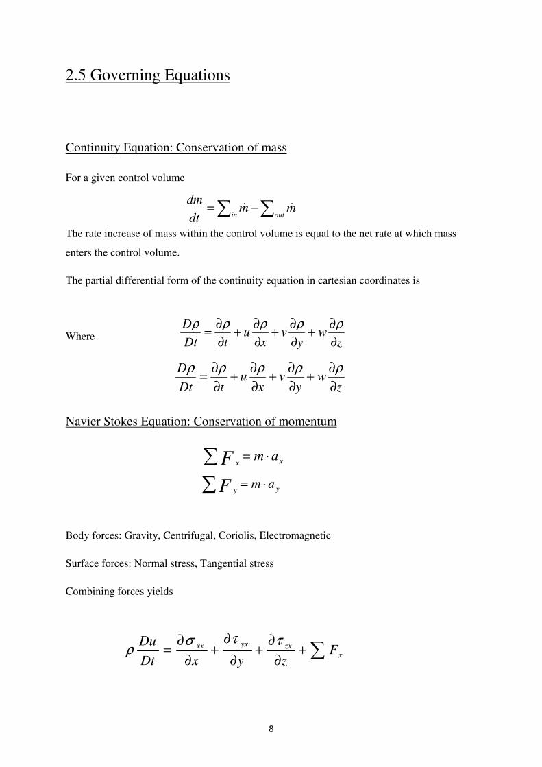
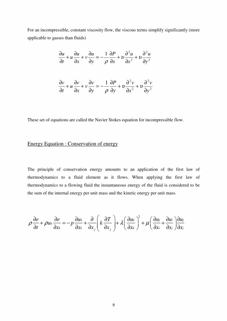
2.5 Governing Equations

Continuity Equation: Conservation of mass

For a given control volume

The rate increase of mass within the control volume is equal to the net rate at which mass

enters the control volume.

The partial differential form of the continuity equation in cartesian coordinates is

Where

Navier Stokes Equation: Conservation of momentum

Body forces: Gravity, Centrifugal, Coriolis, Electromagnetic

Surface forces: Normal stress, Tangential stress

Combining forces yields

∑∑ −=outin

mmdt

dm&&

zw

yv

xu

tDt

D

∂

∂+

∂

∂+

∂

∂+

∂

∂=

ρρρρρ

zw

yv

xu

tDt

D

∂

∂+

∂

∂+

∂

∂+

∂

∂=

ρρρρρ

∑ ⋅= xxamF

∑ ⋅= yyamF

∑+∂

∂+

∂

∂+

∂

∂= x

zxyxxx FzyxDt

Du ττσρ

9

For an incompressible, constant viscosity flow, the viscous terms simplify significantly (more

applicable to gasses than fluids)

These set of equations are called the Navier Stokes equation for incompressible flow.

Energy Equation : Conservation of energy

The principle of conservation energy amounts to an application of the first law of

thermodynamics to a fluid element as it flows. When applying the first law of

thermodynamics to a flowing fluid the instantaneous energy of the fluid is considered to be

the sum of the internal energy per unit mass and the kinetic energy per unit mass.

2k k j i j

k

k k k i j jj j

e e u T u u u uu p k

t x x x x x x x xρ ρ λ µ

∂ ∂ ∂ ∂ ∂ ∂ ∂ ∂ ∂ + = − + + + + ∂ ∂ ∂ ∂ ∂ ∂ ∂ ∂ ∂

2

2

2

21

y

u

x

u

x

P

y

uv

x

uu

t

u

∂

∂+

∂

∂+

∂

∂−=

∂

∂+

∂

∂+

∂

∂υυ

ρ

2

2

2

21

y

v

x

v

y

P

y

vv

x

vu

t

v

∂

∂+

∂

∂+

∂

∂−=

∂

∂+

∂

∂+

∂

∂υυ

ρ

10

2.6 Discretizaton

Conversion of the governing equations into a system of algebraic equations

Two popular discretization techniques in CFD are

1) Finite difference method

In finite difference method, derivatives in the partial differential equation are approximated

by linear combinations of function values at the grid points.

First order derivatives

• Fordward difference

• Backward difference

• Central difference

Second order derivative

• Central difference

For time derivatives

x∆

2+jy

y∆

1+jy

jy

1−jy

2−jy

2−ix 1−ix ix 1+ix 2+ix 3+ix

)(,1,

xOx

uu

x

u jiji∆+

∆

−=

∂

∂ +

)(1,,

xOx

uu

x

u jiji∆+

∆

−=

∂

∂ −

)(2

21,1,xO

x

uu

x

u jiji∆+

∆

−=

∂

∂ −+

))(()(

22

2

,1,,1

2

2

xOx

uuu

x

u jijiji∆+

∆

+−=

∂

∂ −+

)(,,

1

tOt

uu

t

u jin

jin

∆+∆

−=

∂

∂ +

11

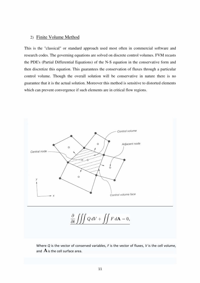
2) Finite Volume Method

This is the "classical" or standard approach used most often in commercial software and

research codes. The governing equations are solved on discrete control volumes. FVM recasts

the PDE's (Partial Differential Equations) of the N-S equation in the conservative form and

then discretize this equation. This guarantees the conservation of fluxes through a particular

control volume. Though the overall solution will be conservative in nature there is no

guarantee that it is the actual solution. Moreover this method is sensitive to distorted elements

which can prevent convergence if such elements are in critical flow regions.

Where Q is the vector of conserved variables, F is the vector of fluxes, V is the cell volume,

and is the cell surface area.

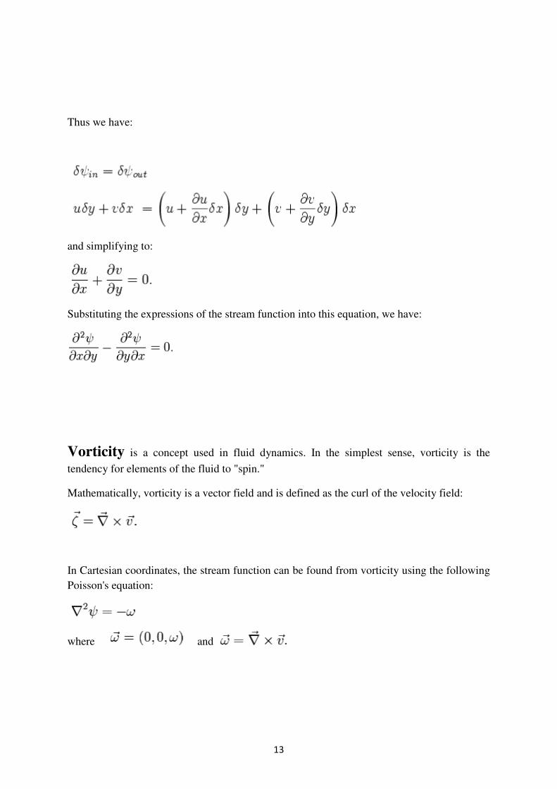
2.7 Stream Function

Stream function ψ for a two dimensional flow is defined such that the flow velocity

can be expressed as:

where

In Cartesian coordinate system this is equivalent to

where u and v are the velocities in the x and y coordinate directions, respectively.

This formulation of the stream function satisfies the t

Consider two dimensional plane flow within a Cartesian coordinate system. Continuity states

that if we consider incompressible flow into an elemental square, the flow into that small

element must equal the flow out of

The total flow into the element is given by:

The total flow out of the element is given by:

12

Stream Function - Vorticity Approach

for a two dimensional flow is defined such that the flow velocity

if the velocity vector

In Cartesian coordinate system this is equivalent to

here u and v are the velocities in the x and y coordinate directions, respectively.

This formulation of the stream function satisfies the two dimensional continuity equation:

Consider two dimensional plane flow within a Cartesian coordinate system. Continuity states

that if we consider incompressible flow into an elemental square, the flow into that small

element must equal the flow out of that element.

The total flow into the element is given by:

The total flow out of the element is given by:

for a two dimensional flow is defined such that the flow velocity

here u and v are the velocities in the x and y coordinate directions, respectively.

wo dimensional continuity equation:

Consider two dimensional plane flow within a Cartesian coordinate system. Continuity states

that if we consider incompressible flow into an elemental square, the flow into that small

13

Thus we have:

and simplifying to:

Substituting the expressions of the stream function into this equation, we have:

Vorticity is a concept used in fluid dynamics. In the simplest sense, vorticity is the

tendency for elements of the fluid to "spin."

Mathematically, vorticity is a vector field and is defined as the curl of the velocity field:

In Cartesian coordinates, the stream function can be found from vorticity using the following

Poisson's equation:

where and

14

Chapter 3

Multigrid Algorithm

15

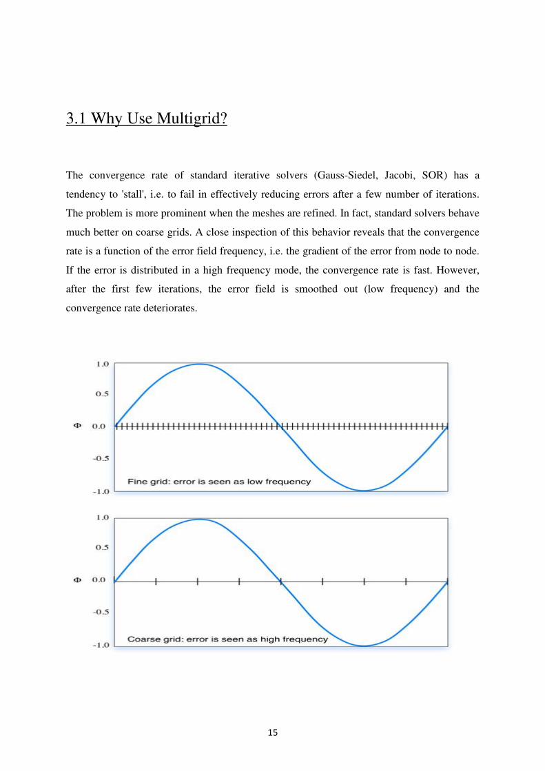
3.1 Why Use Multigrid?

The convergence rate of standard iterative solvers (Gauss-Siedel, Jacobi, SOR) has a

tendency to 'stall', i.e. to fail in effectively reducing errors after a few number of iterations.

The problem is more prominent when the meshes are refined. In fact, standard solvers behave

much better on coarse grids. A close inspection of this behavior reveals that the convergence

rate is a function of the error field frequency, i.e. the gradient of the error from node to node.

If the error is distributed in a high frequency mode, the convergence rate is fast. However,

after the first few iterations, the error field is smoothed out (low frequency) and the

convergence rate deteriorates.

16

3.2 Multigrid Theory

When we solve fluid dynamics, heat transfer or other engineering problems numerically by

using iterative procedures, one of the major issues that concern us is getting a converged

solution on a fine grid. The studies on convergence history of our solution procedure reveal

that in the initial stages of our iterative procedure there is a rapid reduction in residual and as

we march iteratively, the efficiency of smoothing the error falls down and eventually the

solution procedure may stall. Here we will discuss the factors that affect the convergence of

conventional solution procedures on single grid and then study how we can overcome these

problems by using multi-grid algorithms.

Given a set of finite difference equations

Ak

uk

= fk

for a general elliptic equation, any iterative procedure such as Gauss-Seidel, Jacobi,

incomplete LU factorization, etc., is known to converge rapidly for the first few iterations and

very slowly thereafter. Fourier analysis of the error reduction process shows that these

conventional iterative procedures are most efficient in smoothing out the errors of wave

lengths comparable to the mesh size, but are inefficient in removing low frequency

components. However, the low frequency components on any grid are relatively larger on

grids that are coarser than the grid in question. Multi-grid methods seek to exploit the high

frequency smoothing of relaxation methods.

The multi-grid technique is based on the premise that each frequency range of error must be

smoothed on the grid where it is most suitable to do so. Consequently, the multi-grid

technique cycles between coarser and finer grids until all the frequency components of error

are appropriately smoothed. The multigrid concept is distinct from the philosophy of starting

a fine grid solution from an interpolated coarse grid converged solution.

17

In the latter concept, only a better starting guess is provided. Therefore the starting residual

is smaller than a raw guess, but the asymptotic rate of convergence is not improved. The

multi-grid method, on the other hand, cycles between hierarchies of computational grids, so

that error components of all frequency ranges are efficiently removed.

3.3 Basic Algorithm:

Replace problem on fine grid by an approximation on a coarser grid.

Solve the coarse grid problem approximately, and use the solution as a starting guess for the

fine-grid problem, which is then iteratively updated.

Solve the coarse grid problem recursively, i.e. by using a still coarser grid approximation, etc.

18

3.4 Two Dimensional Multigrid System

Multigrid methods are a state-of-the art technique to solve large systems of linear equations A

x = b, where and . This system can be represented as a graph of n

nodes where an edge (i,j) represents a non-zero coefficient. To simplify the following

illustration, we assume that graph to be a regular two dimensional grid. The basic idea of

multigrid is to define a hierarchy of grids as illustrated in the figure. Each node at the coarser

grid level represents a set of nodes at the finer level. Coefficients at some grid level i are

derived from coefficients at grid level i+1 (prolongation) or from coefficients at grid level i-1

(restriction). The grid hierarchy is traversed in V or W-cycles. On each level of the hierarchy

an iterative solver is called.

19

3.5 Numerical Formulation

The residual equation: Let ν be the approximation to the solution of Au=f, where the residual

r=f-Av. Then the error e=u-v satisfies Ae=r.

After relaxing on Au=f on the fine grid, e will be smooth so the coarse grid can approximate

e well. This will be cheaper and e should be more oscillatory there, so relaxation will be more

effective.

Therefore, we go to a coarse grid and relax on the residual equation Ae=r.

3.6 Multigrid Algorithm

Pre smoothing : Relax on Au=f on Ωh to get approximation νh

Computation of residual : Compute r = f - Aνh

Restriction of residual : r2h = Ih2h

rh

Calculation of error : Relax on Ae=r on Ω2h to obtain an approximation to the error, e

2h

Correct the approximation

Post smoothing : Relax on Au=f on Ωh.

hh

h

hheIvv

2

2+→

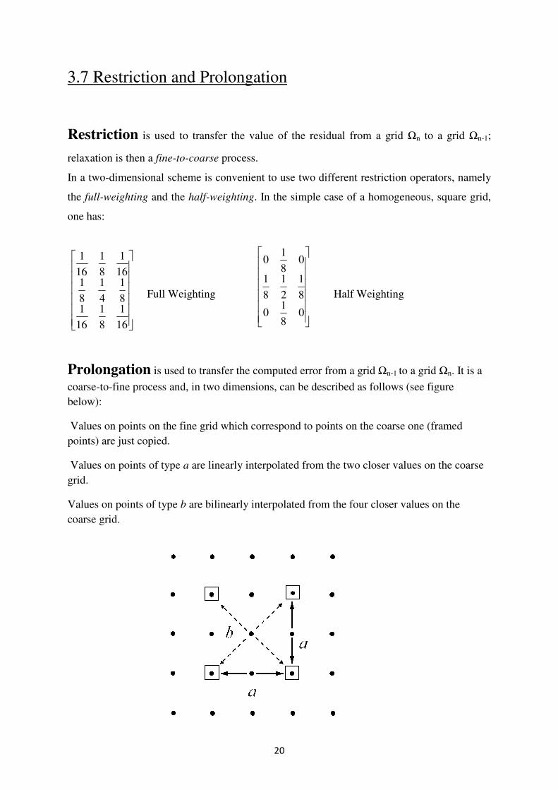
3.7 Restriction and Prolongation

Restriction is used to transfer the value of the residual from a grid

relaxation is then a fine-to-coarse

In a two-dimensional scheme is convenient to use two different restriction operators, namely

the full-weighting and the half

one has:

Full Weighting Half Weighting

Prolongation is used to transfer the computed error from a grid

coarse-to-fine process and, in two

below):

Values on points on the fine grid which correspond to points on the coarse one (framed

points) are just copied.

Values on points of type a are linearly interpolated from the two closer values on

grid.

Values on points of type b are bilinearly interpolated from the four closer values on the

coarse grid.

16

1

8

1

16

18

1

4

1

8

116

1

8

1

16

1

20

Restriction and Prolongation

is used to transfer the value of the residual from a grid

coarse process.

dimensional scheme is convenient to use two different restriction operators, namely

half-weighting. In the simple case of a homogeneous, square grid,

Full Weighting Half Weighting

is used to transfer the computed error from a grid Ωn-1 to a grid

fine process and, in two dimensions, can be described as follows (see figure

Values on points on the fine grid which correspond to points on the coarse one (framed

are linearly interpolated from the two closer values on

are bilinearly interpolated from the four closer values on the

08

10

8

1

2

1

8

1

08

10

is used to transfer the value of the residual from a grid Ωn to a grid Ωn-1;

dimensional scheme is convenient to use two different restriction operators, namely

. In the simple case of a homogeneous, square grid,

Full Weighting Half Weighting

to a grid Ωn. It is a

dimensions, can be described as follows (see figure

Values on points on the fine grid which correspond to points on the coarse one (framed

are linearly interpolated from the two closer values on the coarse

are bilinearly interpolated from the four closer values on the

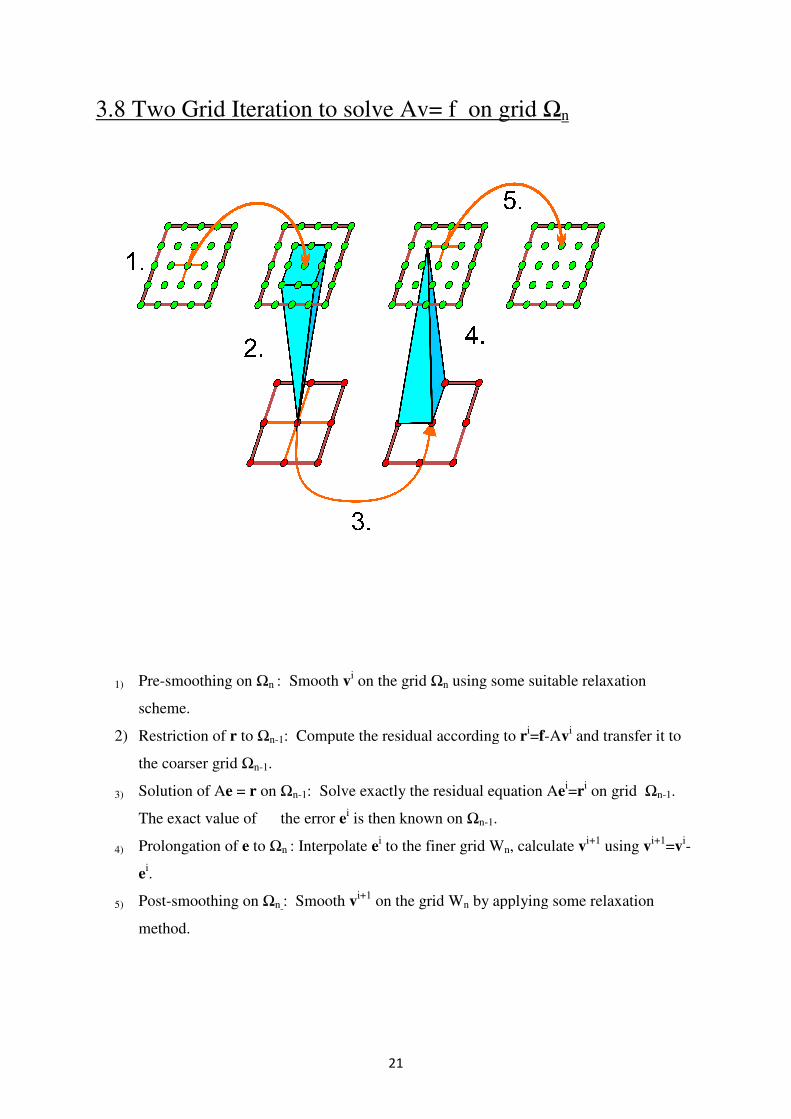
3.8 Two Grid Iteration to solve Av= f on grid

1) Pre-smoothing on Ωn : Smooth

scheme.

2) Restriction of r to Ωn-1: Compute the residual according to

the coarser grid Ωn-1.

3) Solution of Ae = r on Ω

The exact value of the error

4) Prolongation of e to Ωn

ei.

5) Post-smoothing on Ωn : Smooth

method.

21

Two Grid Iteration to solve Av= f on grid Ωn

: Smooth vi on the grid Ωn using some suitable relaxation

: Compute the residual according to ri=f-Av

i

Ωn-1: Solve exactly the residual equation Aei=

The exact value of the error ei is then known on Ωn-1.

n : Interpolate ei to the finer grid Wn, calculate

: Smooth vi+1

on the grid Wn by applying some relaxation

using some suitable relaxation

and transfer it to

=ri on grid Ωn-1.

, calculate vi+1

using vi+1

=vi-

by applying some relaxation

22

Chapter 4

Application and Results

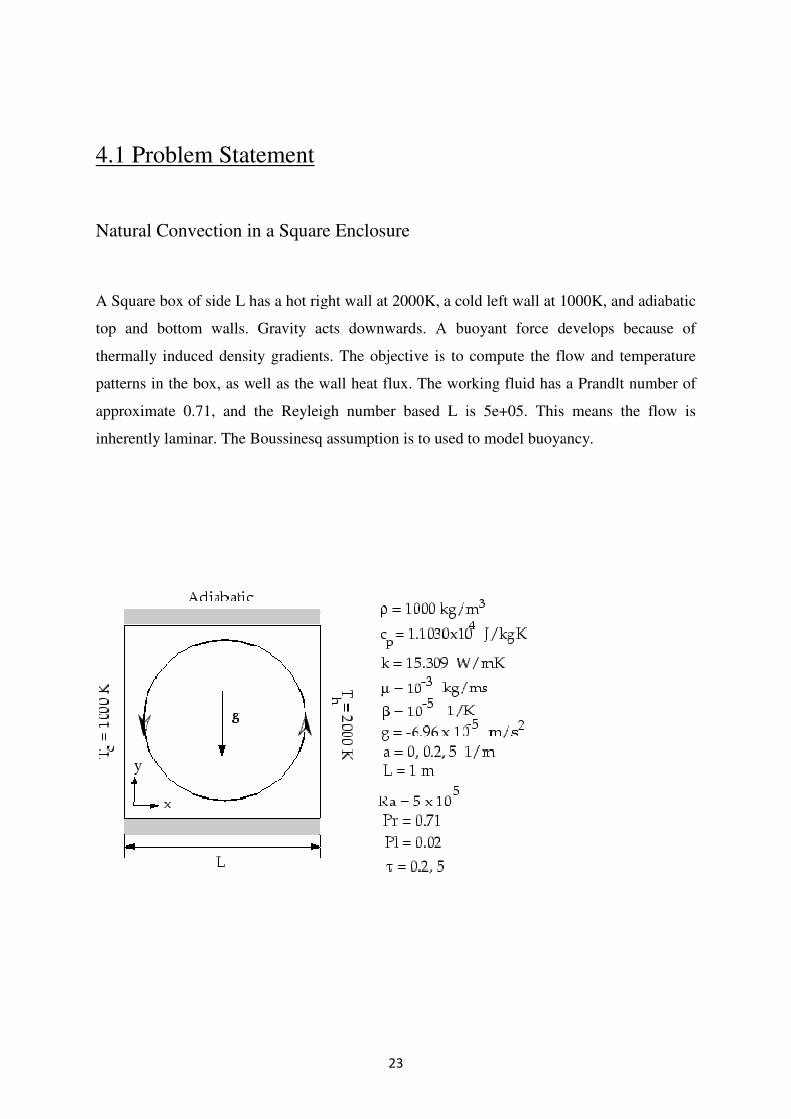
4.1 Problem Statement

Natural Convection in a Square Enclosure

A Square box of side L has a hot right wall at 2000K, a cold left wall at 1000K, and adiabatic

top and bottom walls. Gravity acts downwards. A buoyant force develops because of

thermally induced density gradients. The objective is to compute the flow and temperatu

patterns in the box, as well as the wall heat flux. The working fluid has a Prandlt number of

approximate 0.71, and the Reyleigh number based L is 5e+05. This means the flow is

inherently laminar. The Boussinesq assumption is to used to model buoyancy.

23

4.1 Problem Statement

Natural Convection in a Square Enclosure

box of side L has a hot right wall at 2000K, a cold left wall at 1000K, and adiabatic

top and bottom walls. Gravity acts downwards. A buoyant force develops because of

thermally induced density gradients. The objective is to compute the flow and temperatu

patterns in the box, as well as the wall heat flux. The working fluid has a Prandlt number of

approximate 0.71, and the Reyleigh number based L is 5e+05. This means the flow is

inherently laminar. The Boussinesq assumption is to used to model buoyancy.

box of side L has a hot right wall at 2000K, a cold left wall at 1000K, and adiabatic

top and bottom walls. Gravity acts downwards. A buoyant force develops because of

thermally induced density gradients. The objective is to compute the flow and temperature

patterns in the box, as well as the wall heat flux. The working fluid has a Prandlt number of

approximate 0.71, and the Reyleigh number based L is 5e+05. This means the flow is

inherently laminar. The Boussinesq assumption is to used to model buoyancy.

24

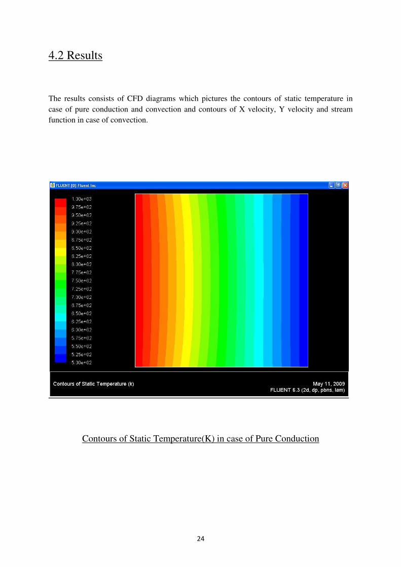
4.2 Results

The results consists of CFD diagrams which pictures the contours of static temperature in

case of pure conduction and convection and contours of X velocity, Y velocity and stream

function in case of convection.

Contours of Static Temperature(K) in case of Pure Conduction

25

Contours of Static Temperature( K) in case of Pure Convection

26

Contours of X velocity (m/s)

Velocity Vectors Coloured By X Velocity( m/s)

27

Contours of Y velocity(m/s)

Velocity Vectors Colored By Y Velocity(m/s)

28

Chapter 5

Conclusion

29

The CFD results obtained using Fluent software were in perfect agreement with the analytical

results. Thus they are verified. Also, the time required to solve the model problem was less

than that taken using the simple grid technique. Multigrid algorithm uses the best of both

coarse and fine grids and thus a fast and accurate result is obtained.

Multigrid techniques have been applied in diverse fields like weather prediction, solid

mechanics, tomography (CAT scan), image segmentation, quantum chemistry and VLSI

design. But multigrid algorithm suffers from certain drawbacks like currently they are several

orders of magnitude slower for non-elliptic steady-state problems. Also it takes careful tuning

to get the algorithm to work on a new problem.

30

References

[1] Nader Ben Cheikh, Natural Convection in a tall enclosure using multigrid method.

Numerical Methods for Partial Differential Equations, Academic Press, New York, Jan 2007

[2] J.Steelant, Multigrid methods for compressible Navier Stokes equation in low speed flows,

Journal of Computational and Apllied Mathematics (1997)

[3] Claudio Cianfrini, Natural convection in tilted square cavities with differentially heated

opposite walls.

[4] Ruben S Montero, Robust multigrid algorithm for the Navier Stokes Equations, Journal of

Computational Physics,173.

[5] A. Brandt, S. McCormick and J. Ruge, Multigrid Methods for Differential Eigenproblems.

SIAM J. Sci. Stat. Comput. 4 (1983), 244-260.

[6] A. Brandt, Multi-grid techniques: 1984 guide with applications to fluid dynamics. GMD-

Studien, St. Augustin, Germany,1984.