A Public Health Approach to Childhood Obesity: The Role of...

A Public Health Approach to Childhood Obesity:

The Role of Econometrics

Laura Gibson

A thesis submitted to the University of Sheffield in fulfilment of the

requirements for the Degree of Doctor of Philosophy

Health Economics and Decision Science

School of Health and Related Research

University of Sheffield

January 2016

Thesis Supervisors:

Dr. Mónica Hernández

Prof. Michael J Campbell, Prof. Michael P Kelly

i

ABSTRACT

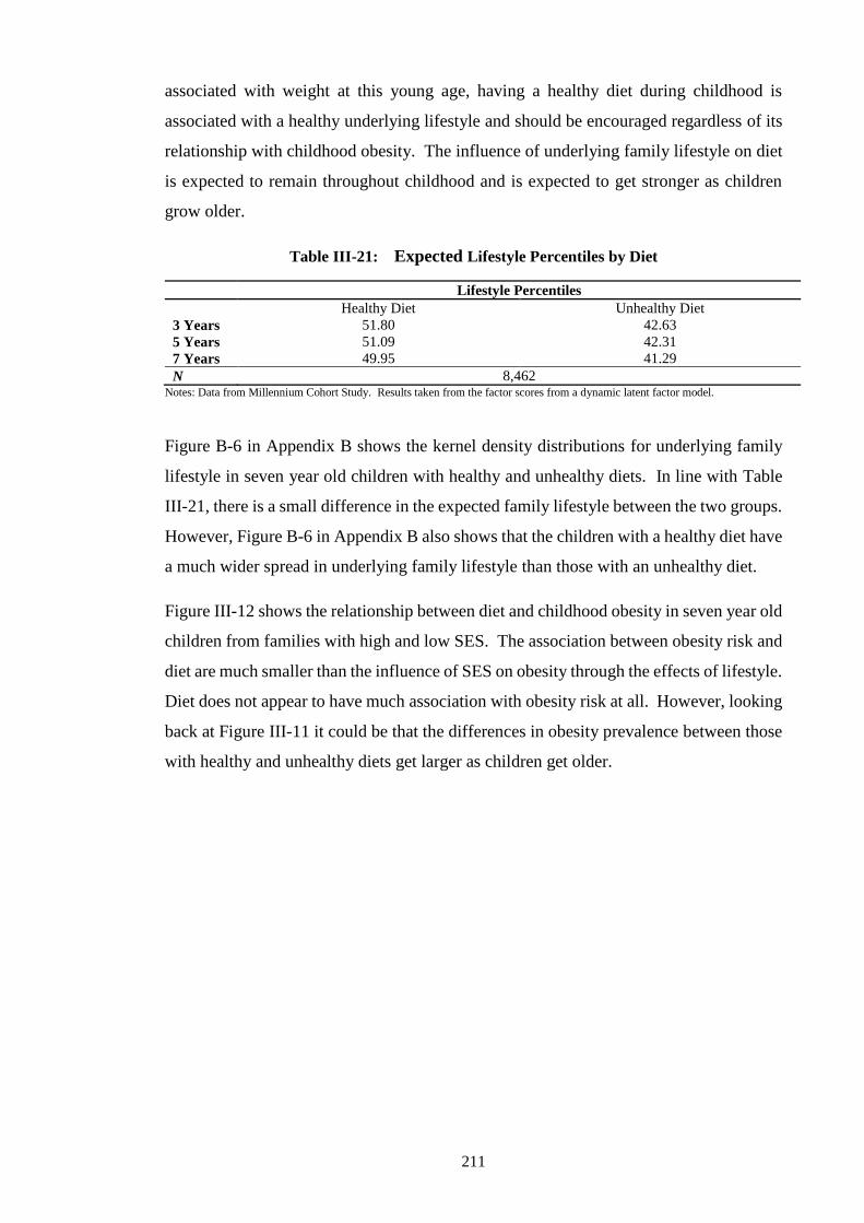
The increasing prevalence of childhood obesity in the United Kingdom is of great interest

to public health policy makers and guidance developers such as NICE, as well as the

general public. In order to develop effective policies, the causes of childhood obesity

need to be better understood. Analysing the Millennium Cohort Survey, this thesis uses

econometric techniques to investigate the relationships between childhood obesity, family

lifestyle behaviours and child health outcomes.

The first empirical chapter investigates the causal effects of breastfeeding behaviours on

obesity during early childhood, a topic which has been of particular interest to NICE.

There is a small but statistically significant influence suggesting that breastfeeding should

be one part of a wider effort to reduce obesity by influencing lifestyle, such as

Change4Life. These effects appear to increase in magnitude and significance as children

get older suggesting that the dynamics of lifestyle and childhood obesity should be

investigated further.

The second empirical chapter investigates the relationship between underlying family

lifestyle and childhood obesity using a dynamic framework. Childhood obesity is one of

the strongest predictors of obesity in adulthood. If lifestyle is learnt in childhood and is

persistent then this could exacerbate the problem of childhood obesity. Amongst other

findings, this chapter concludes that childhood weight status significantly depends on

family lifestyle.

The final empirical chapter extends this model and allows the effects of both family

lifestyle and underlying health on childhood obesity to be investigated. Childhood weight

is a significant outcome measure of underlying child health after the age of five. The

results suggest that policies should target various lifestyle behaviours simultaneously by

improving underlying lifestyle through education and improved understanding and

enabling families to make positive changes.

ii

iii

ACKNOWLEDGEMENTS

My lead supervisor, Dr. Mónica Hernández has provided knowledge, expertise,

invaluable time and support and ongoing encouragement and belief during my time as a

student in ScHARR.

My other supervisors, Professors Mike Kelly and Mike Campbell provided discussion

and ideas for the thesis. Their comments and ongoing advice and support are greatly

appreciated. I would also like to thank the staff at NICE, who made it possible for me to

gain a valuable insight into how their public health guidance is created. I am also very

grateful for my time as a tutor at the University’s Maths and Stats Help (MASH) Service

and would like to thank Chetna Patel and Ellen Marshall for the opportunities and

experiences that they provided me with while studying for a PhD. In addition, I

acknowledge the support I received from Emma Knowles, Rob Barnsley and Stephen

Walters towards the later stages of the PhD process.

My time as a postgraduate research student was made very enjoyable by the other students

in the department. In particular, I would like to thank Sarah Smith, Milad Karimi, Sabine

Grimm and Armando Vargas for being good colleagues and great friends. Thanks also

to my friends from the Department of Economics, in particular, Luke Munford and Helen

Bell, who made Wednesday evenings so much fun.

To finish, I thank my family. My parents, Richard and Ann, have continued to encourage

me to stay at University and study for a PhD. My sister Ellie and best friend Christina

Brady have provided me with valuable time away from studying when it was desperately

needed. Finally, I would like to thank my fiancé Daniel Gray. His love, support, patience

and understanding have been irreplaceable.

iv

I would like to thank the Economics and Social Research Council (ESRC) and the

National Institute for Health and Care Excellence (NICE) for their financial support and

allowing me the opportunity to pursue a PhD. This work was funded by an ESRC CASE

Scholarship [grant number ES/H037977/1].

This thesis uses data from the Millennium Cohort Study1 which is funded by the

Economics and Social Research Council and a consortium of Government departments

and collected by the Centre for Longitudinal Studies at the University of London.

I am grateful to The Centre for Longitudinal Studies, Institute of Education for the use of

these data and to the UK Data Archive and Economic and Social Data Service for making

them available. However, they bear no responsibility for the analysis or interpretation of

these data.

1 University of London. UCL Institute of Education. Centre for Longitudinal Studies, Millennium Cohort Study.

Colchester, Essex: UK Data Archive, January 2012.

v

TABLE OF CONTENTS

ABSTRACT .................................................................................................................................... i

ACKNOWLEDGEMENTS ......................................................................................................... iii

TABLE OF CONTENTS ............................................................................................................... v

LIST OF TABLES ........................................................................................................................ ix

LIST OF FIGURES ................................................................................................................... xiii

LIST OF ACRONYMS ............................................................................................................... xv

I. INTRODUCTION AND RATIONALE ................................................................................ 1

1.1 Obesity and Overweight in Adults ................................................................................. 7

1.1.1 Measuring Adiposity in Adults .............................................................................. 7

1.1.2 Trends in Adult Adiposity ...................................................................................... 8

1.2 Childhood Obesity and Overweight ............................................................................. 12

1.2.1 Measuring Childhood Adiposity .......................................................................... 12

1.2.2 Trends in Childhood Adiposity ............................................................................ 18

1.3 Obesity Policies in the United Kingdom ...................................................................... 20

1.4 Millennium Cohort Study ............................................................................................ 22

1.4.1 Childhood Adiposity Measures in the MCS ........................................................ 25

1.5 Structure and Content of Thesis ................................................................................... 28

II. CHILDHOOD OBESITY AND INFANT FEEDING ......................................................... 33

2.1 Introduction .................................................................................................................. 34

2.2 Literature Review ......................................................................................................... 38

2.2.1 Inconsistency of Measurements ........................................................................... 39

2.2.2 Data and Methods ................................................................................................ 44

2.2.3 Findings ................................................................................................................ 56

2.2.4 Summary .............................................................................................................. 58

2.3 Methodology ................................................................................................................ 59

2.3.1 Selection on Observables ..................................................................................... 60

2.3.2 Removing the Functional Form ........................................................................... 65

2.3.3 Unobservables Confounders: The Potential Problem of Endogeneity ................. 73

2.3.4 Advantages and Disadvantages of Methodologies............................................... 80

2.4 Data .............................................................................................................................. 82

2.4.1 Dependent Variables ............................................................................................ 82

2.4.2 Breastfeeding ....................................................................................................... 83

2.4.3 Independent Variables .......................................................................................... 89

2.4.4 Missing and Excluded Observations .................................................................... 96

2.5 Results ........................................................................................................................ 100

vi

2.5.1 Ordinary Least Squares ..................................................................................... 100

2.5.2 Logit Models ..................................................................................................... 101

2.5.3 Ordered Probit Models ...................................................................................... 104

2.5.4 Regression Model Performance ......................................................................... 107

2.5.5 Propensity Score Matching ................................................................................ 108

2.5.6 Instrumental Variable Estimation ...................................................................... 117

2.5.7 Roy Model ......................................................................................................... 123

2.5.8 Summary of Results........................................................................................... 126

2.6 Discussion and Conclusion ........................................................................................ 129

2.6.1 Comparisons with Existing Literature ............................................................... 129

2.6.2 Policy Implications ............................................................................................ 131

2.6.3 Limitations and Future Research ....................................................................... 133

III. CHILDHOOD OBESITY AND UNDERLYING FAMILY LIFESTYLE ....................... 139

3.1 Introduction ............................................................................................................... 140

3.2 Literature Review ...................................................................................................... 143

3.2.1 Lifestyle Variables and Definitions ................................................................... 144

3.2.2 Determinants of Family Lifestyle ...................................................................... 147

3.2.3 Family Lifestyle and Childhood Obesity ........................................................... 149

3.2.4 Dynamic Modelling of Lifestyle ....................................................................... 152

3.2.5 Family Lifestyle Interventions ........................................................................... 154

3.2.6 Summary ............................................................................................................ 158

3.3 Methodology .............................................................................................................. 160

3.3.1 A Dynamic Latent Factor Model of Family Lifestyle ....................................... 161

3.3.2 Factor Scores ..................................................................................................... 172

3.3.3 Predictions ......................................................................................................... 174

3.4 Data............................................................................................................................ 175

3.4.1 Latent Factors for Family Lifestyle ................................................................... 176

3.4.2 Independent Variables ....................................................................................... 179

3.4.3 Missing and Excluded Observations ................................................................. 185

3.5 Results ....................................................................................................................... 186

3.5.1 Parameter Estimates .......................................................................................... 188

3.5.2 Factor Scores ..................................................................................................... 193

3.5.3 Predictions ......................................................................................................... 195

3.5.4 Summary of Results........................................................................................... 214

3.6 Discussion and Conclusion ........................................................................................ 216



vii

IV. CHILDHOOD OBESITY, FAMILY LIFESTYLE AND CHILD HEALTH ................... 223

4.1 Introduction ................................................................................................................ 224

4.2 Literature Review ....................................................................................................... 226

4.2.1 Measures of Childhood Health........................................................................... 226

4.2.2 Determinants of Childhood Health .................................................................... 229

4.2.3 Childhood Health and Obesity ........................................................................... 231

4.2.4 Childhood Inequalities ....................................................................................... 233

4.2.5 Dynamic Modelling of Health ........................................................................... 235

4.2.6 Summary ............................................................................................................ 244

4.3 Methodology .............................................................................................................. 245

4.3.1 A Dynamic Latent Factor Model ....................................................................... 246

4.3.2 Factor Scores ...................................................................................................... 251

4.3.3 Predictions .......................................................................................................... 253

4.4 Data ............................................................................................................................ 254

4.4.1 Latent Factors for Child Health.......................................................................... 254

4.4.2 Independent Variables ........................................................................................ 258

4.4.3 Missing and Excluded Observations .................................................................. 261

4.5 Results ........................................................................................................................ 261

4.5.1 Parameter Estimates ........................................................................................... 263

4.5.2 Factor Scores ...................................................................................................... 269

4.5.3 Predictions .......................................................................................................... 272

4.6 Discussion .................................................................................................................. 283



V. DISCUSSION .................................................................................................................... 289

5.1 Summary .................................................................................................................... 289

5.2 Policy Implications and the Public Health Approach ................................................ 292

5.3 Future Research ......................................................................................................... 295

5.4 Conclusion ................................................................................................................. 297

REFERENCES .......................................................................................................................... 299

APPENDICES ........................................................................................................................... 317

A. Appendix: Childhood Adiposity and Infant Feeding ......................................................... 319

B. Appendix: Childhood Adiposity and Underlying Family Lifestyle ................................... 353

C. Appendix: Childhood Adiposity, Family Lifestyle and Childhood Health ....................... 363

viii

ix

LIST OF TABLES

Table I-1: WHO Adult BMI Thresholds and Weight Categories .......................................... 8

Table I-2: MSC Timeline ......................................................................................................... 23

Table I-3: Strata and Attrition .................................................................................................. 24

Table I-4: Millennium Cohort Study UK-wide weighting for Strata ....................................... 24

Table I-5: Summary Statistics of Childhood Adiposity Variables .......................................... 27

Table II-1: Dependent Variables used in Each Model .......................................................... 82

Table II-2: Means and Standard Deviations of Continuous Breastfeeding Durations .......... 85

Table II-3: Sample Sizes for Treatment Variables ................................................................ 87

Table II-4: Summary Percentages for Treatment Variables .................................................. 87

Table II-5: Binary Breastfeeding Treatments and BMI at 9 Months .................................... 88

Table II-6: Binary Breastfeeding Treatments and Weight Status ......................................... 89

Table II-7: Descriptive Statistics of Independent Variables ................................................. 95

Table II-8: Number of Observations Excluded ..................................................................... 96

Table II-9: Descriptive Statistics of Childhood Adiposity Variables .................................... 97

Table II-10: Means of Breastfeeding Variables ...................................................................... 98

Table II-11: Descriptive Statistics of Independent Variables ................................................. 99

Table II-12: Summary of Results using OLS ........................................................................ 100

Table II-13: Summary of Results from Logit Models Estimating Obesity ........................... 102

Table II-14: Summary of Results from Logit Models Estimating Overweight..................... 103

Table II-15: Summary of Results from Ordered Probit Models Estimating Weight Category ...

........................................................................................................................... 105

Table II-16: Hypothetical Characteristics for Marginal Effects ............................................ 106

Table II-17: Marginal Effects of Breastfeeding on Obesity in Advantaged and Disadvantaged

Children ............................................................................................................. 106

Table II-18: RESET tests for Misspecification in OLS Regressions .................................... 107

Table II-19: Link Tests from Standard Regression Models .................................................. 108

Table II-20: Probit Models Estimating Propensity Scores of Breastfeeding Treatments at Age

3......................................................................................................................... 110

Table II-21: Link Tests in Calculating the Propensity Score ................................................ 112

Table II-22: ATEs on Adiposity Outcomes using PSM ........................................................ 114

Table II-23: Standard OLS Regressions including the Instrument ....................................... 118

Table II-24: Summary of First Stage IV Results ................................................................... 119

Table II-25: Cragg-Donald Wald Tests for Weak Instruments ............................................. 120

Table II-26: Anderson-Rubin Tests for Weak Instruments ................................................... 121

Table II-27: Summary of Second Stage IV Results .............................................................. 121

Table II-28: Test for Endogenous Treatments ...................................................................... 122

Table II-29: Roy Model Estimated Treatment Effects .......................................................... 124

Table II-30: Roy Model Predicting Treatment ...................................................................... 125

Table II-31: LR Test for Endogeneity ................................................................................... 125

Table III-1: Outcome Measures of Underlying Family Lifestyle ......................................... 177

Table III-2: Independent Determinants of Underlying Family Lifestyle ............................. 179

Table III-3: Independent Determinants of Childhood Adiposity Measures ......................... 182

Table III-4: Model Fit Statistics ........................................................................................... 188

Table III-5: Estimated Factor Loadings ................................................................................ 189

Table III-6: Estimated Coefficients in Predicting Latent Family Lifestyle .......................... 190

Table III-7: Estimated Coefficients in Childhood Adiposity ............................................... 191

Table III-8: Standardised Factor Loadings ........................................................................... 192

x

Table III-9: Standardised AR Parameters ............................................................................. 192

Table III-10: Proportion of Families Remaining in Initial Lifestyle Percentile Group ........... 193

Table III-11: Proportion of Families Remaining in Initial Lifestyle Percentile Group (2) ..... 194

Table III-12: Correlations between Factors Scores ................................................................. 194

Table III-13: Differences between High and Low Family Lifestyle Rankings ....................... 195

Table III-14: Independent Characteristics of Hypothetical Children ...................................... 196

Table III-15: Expected Lifestyle Percentiles by Ethnicity ...................................................... 198

Table III-16: Expected Lifestyle Percentiles by Family Structure .......................................... 202

Table III-17: Expected Lifestyle Percentiles in Advantaged and Disadvantaged Children .... 204

Table III-18: Expected Lifestyle Percentiles by Parental Weight in High SES ...................... 207

Table III-19: Expected Lifestyle Percentiles by Parental Weight in Low SES ....................... 207

Table III-20: Expected Lifestyle Percentiles by Lifestyle during Pregnancy ......................... 208

Table III-21: Expected Lifestyle Percentiles by Diet .............................................................. 211

Table III-22: Expected Lifestyle Percentiles at Seven Years by Physical Activity ................ 213

Table IV-1: Outcome Measures of Underlying Child Health and Family Lifestyle ............. 256

Table IV-2: Independent Determinants of Underlying Child Health .................................... 259

Table IV-3: Stages of Childhood........................................................................................... 261

Table IV-4: Model Fit Statistics ............................................................................................ 262

Table IV-5: Estimated Factor Loadings for Child Health ..................................................... 264

Table IV-6: Parameter Estimates of Independent Variables on Family Lifestyle and Child

Health, 𝛽 and 𝜚 .................................................................................................. 265

Table IV-7: Autoregressive Parameter Estimates ................................................................. 265

Table IV-8: Parameter Estimates of Independent Variables Predicting Adiposity Measures, 𝛿.

........................................................................................................................... 267

Table IV-9: Standardised Factor Loadings for Latent Child Health Factors ........................ 268

Table IV-10: Standardised AR Processes ............................................................................... 269

Table IV-11: Proportion of Families Remaining in Initial Child Health Percentile Group .... 269

Table IV-12: Proportion of Families Remaining in Initial Child Health Percentile Group (2) .....

........................................................................................................................... 270

Table IV-13: Correlations between Factors Scores ................................................................. 271

Table IV-14: Differences between Children with Excellent and Poor Health ........................ 272

Table IV-15: Independent Characteristics of Hypothetical Children ...................................... 273

Table IV-16: SES and Expected Factor Percentiles ................................................................ 274

Table IV-17: Correlation between Birth Weight and Child Health......................................... 275

Table IV-18: Expected Health Percentiles in Children with differing Birth Weight .............. 277

Table IV-19: Expected Health Percentiles by Child’s Diet ..................................................... 279

Table IV-20: Expected Health Percentiles by Child’s Physical Activity at 7 Years ............... 280

Table IV-21: Expected Health Percentiles by Infant Feeding and Growing at 7 Years .......... 282

Table IV-22: Expected Infant Feeding and Lifestyle Percentiles at 7 Years .......................... 282

Table A-1: Studies included in the Literature Review ......................................................... 320

Table A-2: Description of Independent Variables ............................................................... 325

Table A-3: Linear Models Estimating BMI in Three Year Olds ......................................... 326

Table A-4: Linear Model Estimating BMI in Five Year Olds ............................................. 327

Table A-5: Linear Model Estimating BMI in Seven year Olds ........................................... 328

Table A-6: Logit Model Estimating Overweight in Three Year Olds ................................. 329

Table A-7: Logit Model Estimating Overweight in Five Year Olds.................................... 330

Table A-8: Logit Model Estimating Overweight in Seven Year Olds ................................. 331

Table A-9: Logit Model Estimating Obesity in Three Year Olds ........................................ 332

Table A-10: Logit Model Estimating Obesity in Five Year Olds .......................................... 333

Table A-11: Logit Model Estimating Obesity in Seven Year Olds ....................................... 334

xi

Table A-12: Breastfeeding on Weight Status at 3 Years using Ordered Probit Models ....... 335



Table A-15: Propensity Score Matching with Outcome BMI ............................................... 338

Table A-16: Propensity Score Matching with Binary Outcome Obesity .......................... 339

Table A-17: Propensity Score Matching with Binary Outcome Overweight .................... 340

Table A-18: First Stage of 2SLS Estimating Breastfeeding in Three Year Olds .................. 341

Table A-19: First Stage of 2SLS Estimating Breastfeeding in Five Year Olds .................... 342

Table A-20: First Stage of 2SLS Estimating Breastfeeding in Seven Year Olds .................. 343

Table A-21: Second Stage of 2SLS Estimating BMI in Three Year Olds ............................ 344

Table A-22: Second Stage of 2SLS Estimating BMI in Five Year Olds............................... 345

Table A-23: Second Stage of 2SLS Estimating BMI in Seven Year Olds ............................ 346

Table A-24: Roy Model (Age 3 Years) ................................................................................. 347



Table B-1: Summary Statistics for Final Sample ................................................................ 354

Table B-2: Mplus Output for Lagged Influence on Child Weight Status ........................... 355

Table B-3: Threshold Parameters for Lifestyle Outcome Measures ................................... 357

Table C-1: Summary Statistics for Final Model ................................................................. 364

Table C-2: Mplus Output for Lagged Influences on Child Weight Status .......................... 366

Table C-3: Estimated Factor Loadings for Family Lifestyle .............................................. 370

Table C-4: Threshold Parameters for Family Lifestyle Outcome Measures ....................... 371

Table C-5: Threshold Parameters for Child Health Outcome Measures ............................. 372

xii

xiii

LIST OF FIGURES

Figure I-1: Average BMI of English Males and Females (1993-2009) .................................. 9

Figure I-2: Percentage of English Adults Overweight or Obese (1993 and 2009) ............... 10

Figure I-3: Percentage of English Adults by BMI Category (1993 - 2009) .......................... 10

Figure I-4: BMI Percentiles for US Boys between Two and Twenty Years ......................... 13

Figure I-5: BMI Percentiles for US Girls between Two and Twenty Years ......................... 14

Figure I-6: Percentage of UK Children who are Obese (1995-2012) ................................... 19

Figure I-7: Median BMI by Age and Sex from the CDC Growth Charts and Children from

the MCS. ............................................................................................................. 28

Figure II-1: Percentage of Children Breastfed by Duration ................................................... 86

Figure III-1: Path Diagram .................................................................................................... 184

Figure III-2: Expected Mean Weight (kg) at first MCS Interview by Ethnicity .................... 197

Figure III-3: Expected Prevalence of Obesity in Male Children by Ethnicity ....................... 198

Figure III-4: Expected Weight at Nine Months by Family Structure .................................... 200

Figure III-5: Expected Prevalence of Obesity by Family Structure (2) ................................. 201

Figure III-6: Expected Prevalence of Obesity for Advantaged and Disadvantaged Child .... 203

Figure III-7: Expected Childhood Obesity and Parental Weight Status (High SES) ............. 205

Figure III-8: Expected Childhood Obesity and Parental Weight Status (Low SES) ............. 206

Figure III-9: Expected Maternal Lifestyle and Childhood Obesity ....................................... 208

Figure III-10: Expected Maternal Lifestyle and Childhood Obesity (2).............................. 209

Figure III-11: Expected Diet and Childhood Obesity .......................................................... 210

Figure III-12: Expected Diet and Childhood Obesity by SES at 7 Years ............................ 212

Figure III-13: Expected Physical Activity and Childhood Obesity at 7 Years .................... 213

Figure III-14: Expected Physical Activity and Childhood Obesity by SES at 7 Years ....... 214

Figure IV-1: Path Diagram .................................................................................................... 260

Figure IV-2: Expected Childhood Obesity and Socioeconomic Status ................................. 274

Figure IV-3: Expected Birth Weight and Subsequent Childhood Obesity ............................ 276

Figure IV-4: Expected Diet, Childhood Obesity and Maternal Education at 7 Years ........... 278

Figure IV-5: Expected Physical Activity, Childhood Obesity and Maternal Education at 7

Years ................................................................................................................. 279

Figure IV-6: Expected Infant Feeding and Childhood Obesity in Advantaged and

Disadvantaged Children .................................................................................... 281

Figure B-1: Kernel Densities of Lifestyle by Ethnicity ........................................................ 358

Figure B-2: Kernel Densities of Lifestyle by Family Structure ........................................... 359

Figure B-3: Kernel Densities of Lifestyle by Advantaged and Disadvantaged .................... 359

Figure B-4: Kernel Densities of Lifestyle by Parental Weight and SES .............................. 360

Figure B-5: Kernel Densities of Lifestyle by Lifestyle during Pregnancy ........................... 361

Figure B-6: Kernel Densities of Lifestyle by Diet................................................................ 361

Figure B-7: Kernel Densities of Lifestyle by Physical Activity ........................................... 361

Figure C-1: Kernel Densities of Health by Socioeconomics Status ..................................... 373

Figure C-2: Kernel Densities of Health by Birth Weight ..................................................... 373

Figure C-3: Kernel Densities of Health by Diet ................................................................... 373

Figure C-4: Kernel Densities of Health by Physical Activity .............................................. 374

Figure C-5: Kernel Densities by Infant Feeding and Growing Characteristics .................... 374

xiv

xv

LIST OF ACRONYMS

2SLS Two-Stage Least Squares

AIC Akaike Information Criterion

ALSPAC Avon Longitudinal Study of Pregnancy and Children

ANOVA Analysis of Variance

AR Autoregressive

AROW At Risk of Overweight

ATE Average Treatment Effect

ATT Average Treatment Effect on the Treated

ATU Average Treatment Effect on the Untreated

BHPS British Household Panel Survey

BIC Bayesian Information Criterion

BIV Biological Implausible Value

BMI Body Mass Index

CDC Centre for Disease Control and Prevention

CDF Cumulative Distribution Function

CDS Child Development Supplement

CHQ Childhood Health Questionnaire

CIA Conditional Independence Assumption

CSDH Commission of Social Determinants of Health

CVD Cardiovascular Disease

DH Department of Health

EFA Exploratory Factor Analysis

GAM General Additive Model

GEE Generalised Estimating Equations

GPS Generalised Propensity Score

HDA Health Development Agency

HSE Health Survey for England

HTA Health Technology Appraisal

IID Independently and Identically Distributed

IOTF International Obesity Taskforce

IQ Intelligence Quotient

IV Instrumental Variable

kg kilograms

LR Likelihood Ratio

m meters

MCS Millennium Cohort Study

MTA Multiple Technology Appraisal

NCDS National Child Development Study

NCHS National Center for Health Statistics

NHS National Health Service

NICE National Institute of Health and Care Excellence

NN Nearest Neighbour

NS-SEC National Statistics Socioeconomic Classification

NVQ National Vocational Qualification

OLS Ordinary Least Squares

PHE Public Health England

PROBIT Promotion of Breastfeeding Intervention Trial

PSM Propensity Score Matching

RCPCH Royal College of Paediatric and Child Health

RCT Randomised Controlled Trial

RESET Regression Equation Specification Error Test

SAH Self-assessed Health

xvi

SACN Scientific Advisory Committee on Nutrition

SES Socioeconomic Status

STA Single Technology Appraisal

UK United Kingdom

UNICEF United Nations Children’s Fund

US United States

WAPCS Western Australian Pregnancy Cohort Study

WHO World Health Organisation

ZINB Zero-Inflated Negative Binomial

ZIP Zero-Inflated Poisson

xvii

1

I. INTRODUCTION AND RATIONALE

2

Childhood obesity has been increasing in prevalence in the United Kingdom (UK) over

the past three decades, causing high levels of public interest as well as government

concern. In order to develop effective policies, the causes and consequences of obesity

during childhood need to be fully understood. Surprisingly, relatively little is known

about the effects of childhood obesity caused by early childhood influences. Childhood

obesity is also a growing public health concern and due to the numbers of obese children

a population based public health approach is needed rather than an individual clinical

approach.

The World Health Organisation (WHO) defines public health as the prevention of disease,

promotion of health and prolonging of life among the population as a whole. The aim of

any public health approach is to benefit the population of interest, in this case, as many

children in the UK as possible, by tackling the underlying risk factors of a disease at a

population level. In England, it is the role of the National Institute of Health and Care

Excellence (NICE) to create public health guidance2. This guidance is developed

independently of the Government by committees of experts and members of the public

who review the available evidence in order to make recommendations. NICE produce

advice and guidance on a range of public health issues aimed at the public, the National

Health Service (NHS), other health bodies and local authorities as well as other

organisation in both the public, private and voluntary sectors3.

The majority of public health guidance developed by NICE uses economic models which

predict future health or economic outcomes as consequences of different potential

interventions, actions or policies. These include cost-effectiveness models usually based

on the principles of cost utility analysis which aim to identify interventions that will have

benefits beyond their cost of implementation. These economic models are evidence based

wherever possible but inevitably also rely on a number of assumptions where evidence is

lacking. Where needed, these assumptions are tested using sensitivity analysis. They

collate clinical, medical, economic and policy related evidence from a range of sources.

Evidence is often taken from clinical trials and policy evaluation or econometric studies.

Much of this evidence is of short-term outcomes; for example, trials do not routinely

collect information longer than two years after an intervention. However, for policy

purposes it is just as important, if not more, to understand how these effects come about

2 NICE primarily produces guidance for England, but has agreements to provide certain guidance and recommendations

to Scotland, Wales and Northern Ireland also. 3 NICE also provides guidance on other health and care related topics, such as health technology appraisals (HTAs)

and multiple technology appraisals (MTAs) as well as clinical and social care guidelines.

3

and develop over time. To overcome this problem, econometric models can be used to

provide more long-term evidence. NICE guidance and recommendations can benefit

greatly from this knowledge, particularly when assessing cost-effectiveness which

requires long-term outcomes to be predicted. Where this evidence is not available,

economic models must extrapolate and/or make assumptions. The more evidence

available on longer-term outcomes relating to any public health guidance, the more

accurate the economic assessment or cost-effective analysis can be.

An example of a ‘Public Health Approach’ is defined by WHO (2015) as a four-step

iterative approach. The four steps are outlined as follows:

1. Surveillance. What is the problem that we aim to solve? In this case it is

childhood obesity.

2. Determinants. What are the causes? Are there influences which protect against

childhood obesity or which are risk factors for childhood obesity?

3. Informing interventions. What policies work and who benefits most from each of

these policies? What types of children will benefit most from the proposed

interventions?

4. Implementation. Carrying out the interventions on a larger scale in order to

prevent childhood obesity at a national or international level.

This thesis aims to contribute to steps two and three of this public health approach. The

scope of this thesis does not include any analysis which addresses steps one or four,

although these are discussed in the introductory sections and literature reviews.

Current practice in public health broadly focuses on evidence relying expert opinion or

data from other countries or unrepresentative samples. This thesis uses a large nationally

representative dataset which allows analysis to be applicable to the UK population and

enables a variety of children with different characteristics to be investigated. The role of

econometrics in producing evidence for public health guidance is two-fold. On one hand

it can inform public health recommendations and directly influence expert committees to

help them in the development of public health guidance. This is generally done by

estimating econometric models using observational data in order to identify the effects of

past interventions or treatments, usually, but not always, on a single outcome. On the

other hand, econometric analysis can be used to inform the economic models which are

4

then used to create guidance or recommend interventions. Any type of econometric

model can be used to feed into these economic models, but certain econometric models,

known as structural models, are particularly useful. This is because they estimate systems

of equations as well as the correlations between them and thus any subsequent economic

model needs to make no assumptions about these correlations. More complex

econometric analysis involving multiple outcomes over a period of time using

longitudinal data can provide longer-term evidence. This type of model is known in

statistics as a structural model and can lead to more solid and robust public health

interventions being recommended. These structural models pull together related concepts

providing more evidence for economic models and guidance developers. They also allow

the distributions of treatment effects to be given more consideration (Carneiro, Hansen,

& Heckman, 2003; Heckman & Urzúa, 2010). This means that rather than identifying

the average effect of an intervention on a chosen outcome measure or a set of outcome

measures independently, it is possible to explore how different individuals might be

influenced differentially by potential interventions, allowing different parameter

estimates to answer different policy questions using a single model. The need for more

robust long-term evidence to feed into economic or cost-effectiveness models is growing

as the NHS budget is being increasingly stretched. Therefore it is more important as ever

that long-term effects are identified.

There are a number of examples of econometric evidence which have been used in public

health guidance over recent years. For example, Pilgrim et al. (2010) carried out a

systematic review of econometric studies which investigated the long-term influences of

teenage pregnancy. Their review only included studies which used econometric

techniques which controlled for unobservable confounders. This review emphasised the

benefits of long-term outcomes being investigated and used in a public health setting.

However, it also highlighted the lack of dynamic models used to investigate outcomes

over time; none of the identified studies used outcomes which were measured at more

than one point in time. Similarly, most of the studies identified by this review estimated

population average effects which limits the evidence available for economic models and

does not allow the distribution of effects to be investigated. Other studies identified in

this review estimated the local average treatment effect, which is also problematic for

NICE (Faria et al., 2015) because these studies only estimate the effect for a subgroup of

the population. This review of econometric studies was used as evidence in public health

guidance on contraception for young people (NICE, 2014b).

5

Other studies which have used econometric methods and which have been used as

evidence to support public health guidance include Brennan et al. (2008) and Brown &

Taylor (2008). Brennan et al. (2008) used econometric analysis to estimate the effects of

alcohol pricing and promotion policies on underage drinking, binge drinking and harmful

drinking. Their intention was to help inform an economic model where a lack of evidence

was identified; previously, there was no econometric analysis in this area which was fit

for purpose. In this report, the authors investigated the price elasticities of different types

of alcohol using cross-sectional data. Their results were used to inform an economic

model which predicted the effects of different alcohol pricing policies. This economic

model was then used to update evidence in public health guidance on alcohol-use

disorders (NICE, 2014a). However, the economic model was limited in that there was a

lack of evidence on long-term influences and as a result the economic model was unable

to estimate the long-term effects of alcohol pricing policies without the need for

extrapolation and additional assumptions.

Brown & Taylor (2008) carried out econometric analysis on the long-term effects of

bullying during childhood on educational attainment and income. Although this article

was not originally intended to be used as evidence for NICE or other public health bodies,

it nevertheless had an impact on public health guidance. Evidence from this study was

used in an economic model by Hummel et al. (2009) to provide NICE with an economic

cost-effectiveness model for emotional and social wellbeing interventions in secondary

schools (NICE, 2012b). Although this study used static models and did not investigate

how these influences came about, it provided an important addition to the existing

evidence which was otherwise limited to short-term outcomes.

More complex econometric models have also been drawn upon to feed into economic

models used in NICE guidance. For example, public health guidance on childhood

development (NICE, 2012b) relied heavily on an econometric structural model developed

by Hernandez Alava et al. (2011) to investigate long-term outcomes which resulted from

childhood cognitive, social and emotional development. This report used a range of

datasets, including the Millennium Cohort Study (MSC) for which a variety of outcomes

were jointly analysed. These outcomes included both child outcome measures (in the

MCS) and adult outcomes (in other datasets) and depended on either behaviour and/or

cognition in children at different ages. This information was then incorporated into an

economic model developed by Hummel et al. (2011) allowing the influence of social and

emotional wellbeing interventions on outcome measures at age five and on adult

6

outcomes to be predicted. The dynamic nature of these models provide more information

than simpler static models and enable more than one equation to be jointly estimated at

multiple time points and allow the analysis of a range of outcomes simultaneously.

This thesis uses a range of econometric techniques to investigate the relationships

between childhood obesity, family lifestyle behaviours and child health outcomes. It aims

to identify the causes of childhood obesity during early childhood in order to inform

policy and tackle the childhood obesity epidemic. It investigates childhood obesity using

methods which have not before been used in these settings in an attempt to identify causal

relationships. In addition, many of the parameters investigated in this thesis have not

previously been considered. This thesis consists of three distinct but related empirical

chapters, each analysing data from the Millennium Cohort Study (Centre for Longitudinal

Studies, 2000-2008). Each of the chapters have important policy implications and each

could be used to enrich future public health guidance provided by NICE and add to the

public health debate.

Chapter II investigates the effects of breastfeeding behaviours on childhood obesity

throughout the early years of life, using a variety of econometric models. It uses a number

of models in order to find the most appropriate set of assumptions for this empirical

problem and to check the robustness of the results. The chapter aims to identify causal

influences with the intention of informing public health guidance development

committees such as those interested in producing guidance to reduce childhood obesity

or increase breastfeeding participation. For example, this type of econometric analysis

could have been beneficial to committees developing recent public health guidance on

how to improve lifestyle to prevent and reduce childhood obesity (NICE, 2013b), tackle

obesity in local communities (NICE, 2012c) and improve maternal and child nutrition

(NICE, 2008). In addition, any results from this chapter also have the potential to be used

in economic models for obesity.

Chapter III and Chapter IV use structural models to investigate the underlying causes of

childhood obesity. Chapter III explores the causal influence of underlying family lifestyle

on childhood obesity and how this relationship develops over time. Chapter IV introduces

underlying childhood health to the model used in Chapter III in order to determine the

extent to which poor health during childhood influences childhood obesity. In addition

to the contributions to the public health debate described above for Chapter II, these two

empirical chapters have the potential to provide economic models with a wealth of

7

information about a number of different outcomes, over and above childhood obesity.

For example, the structural model in Chapter III jointly estimates the weight status of the

child and of their parents as well as other outcome measures and as a result, findings from

this study could provide important evidence in future public health guidance on obesity

in a family context. Similarly, variables relating to diet, exercise and a variety of

childhood health conditions are estimated by these models highlighting the wide range of

public health guidance which could benefit from these structural models.

Results from the thesis suggest that longer breastfeeding durations reduce childhood BMI

and the likelihood of childhood obesity. These effects become more apparent as children

get older. The analysis reveals that childhood weight is strongly influenced by family

lifestyle which also has strong influences on parental weight status, in particular maternal

weight status. Childhood weight is causally influenced by underlying health but not to

the same extent as family lifestyle. The results suggest that policies should focus on a

wide range of lifestyle behaviours simultaneously by enabling families to make changes

and educating them to understand why healthy lifestyles are important and how they

impact on health and adiposity. By targeting disadvantaged families, socioeconomic

inequalities in health and obesity prevalence during childhood could be reduced.

The remainder of this chapter discusses the recent trends in obesity in the UK. It also

explains the reasons for using childhood obesity and overweight definitions which are

different to adult definitions. It illustrates the need for high quality research in the area

of childhood obesity, obesity policies which are already in place in the UK and describes

what this thesis will do to add to the existing literature and contribute to knowledge in

this area.

1.1 Obesity and Overweight in Adults

1.1.1 Measuring Adiposity in Adults

The most commonly used and accepted measurement of adult adiposity is Body Mass

Index (BMI), which calculated using weight in kilograms (kg) and height in meters (m),

𝐵𝑀𝐼 =𝑤𝑒𝑖𝑔ℎ𝑡 (𝑘𝑔)

ℎ𝑒𝑖𝑔ℎ𝑡 (𝑚2). (I.1)

8

BMI can then be used to categorise adult individuals into different weight status; for

example, underweight, normal weight, overweight and obese. The WHO classifications

of weight status in adults are shown in Table I-1.

Table I-1: WHO Adult BMI Thresholds and Weight Categories

Source: World Health Orgnaisation (2011c). Notes: Definitions of weight status in adults.

Definitions of overweight and obesity are designed to identify individuals carrying excess

body fat. According to the Department of Health (DH) (2010), an acceptable level of

body fat in adults differs between individuals depending on their height and sex.

However, neither BMI nor the most commonly used classifications for overweight or

obesity in adults take sex into account. Greene et al. (2008) explained that the current

BMI boundaries do not give the correct evaluation of adiposity of certain types of people.

For example, athletic individuals are likely to have more heavy muscle and might fall into

the overweight category with much less body fat than someone with a normal build.

Similarly, elderly people are likely to have less muscle and therefore might be

miscategorised in a lower BMI category when they experience the same health risks as

overweight or obese individuals. Individuals misclassified as normal could potentially

have health risks which are being ignored. Despite this, BMI remains the most widely

used measure of adult adiposity and no better alternative has yet been agreed upon.

1.1.2 Trends in Adult Adiposity

In 2011, WHO (2011a) estimated that 67.8% and 63.8% of male and female UK adults,

respectively, were overweight and 23.7% and 26.3%, respectively, were obese. Obesity

has become one of the biggest health problems faced by developed countries and the rate

at which obesity is continuing to increase remains alarming. The past twenty years has

seen obesity double worldwide and in 2008 an estimated 1.5 billion adults worldwide

were classified as overweight or obese. Obesity during childhood has been repeatedly

found to be one of the strongest predictors of obesity in adulthood. Therefore, learning

Body Mass Index (BMI) Weight Status

BMI < 18.5 Underweight

18.5 ≤ BMI < 25 Normal weight

25 ≤ BMI < 30 Overweight

30 ≤ BMI < 35 Obese class I

35 ≤ BMI < 40 Obese class II

BMI ≥ 40 Obese class III

9

how to tackle obesity in early life is important in the fight against obesity in the entire

population.

Using data from the Health Survey for England (HSE) accessed through the National

Health Service (NHS) Information Centre website (2008), Figure I-1, Figure I-2 and

Figure I-3 show the evolution of body mass index (BMI) in the population of England

over recent years. Figure I-1 shows the increase in mean BMI in England for both male

and female adults since 1993. The average BMI has steadily increased over this short

period of time from under 26 to over 27 and in 2009 the average BMI among women

surpassed that of men for the first time; this could be of particular importance to policy

makers if the reasons for this change are identified. For example, it could be a result of

lifestyle changes in men and women. Figure I-1 shows that since 1993, the average BMI

for both men and women has remained above 25, the threshold for the definition of

overweight.

Figure I-1: Average BMI of English Males and Females (1993-2009)

Source: Health Survey for England, NHS Information Centre website, (The NHS Information Centre 2008). Notes: Mean BMI of

English Male and Female Adults over the age of sixteen years between 1993 and 2009.

Figure I-2 compares the percentage of adults in England who were considered overweight

or obese in 1993 and 2009. During these years, overweight and obesity increased in adults

of all ages. In both 1993 and 2009, there is a peak in the population of overweight adults

between their fifties and sixties before it decreases in older adults. This peak occurs at an

older age in 2009 than in 1993, possibly due to increases in life expectancy between the

two periods and the worsening of the obesity epidemic.

24.5

25.0

25.5

26.0

26.5

27.0

27.5

BM

I

Year

Average Male BMI

Average Female BMI

10

Figure I-2: Percentage of English Adults Overweight or Obese (1993 and 2009)

Source: Health Survey for England, NHS Information Centre website, (The NHS Information Centre 2008). Notes: Percentage of English adults (sixteen years or over) which are considered overweight or obese between 1993 and 2009.

Figure I-3 shows the changes in the percentage of English adults in each weight

category between 1993 and 2009. The percentage of underweight and overweight

adults remained relatively stable over time, at around 1.5% and 38%, respectively.

However, while the percentage of normal weight adults decreased, the percentage of

obese adults increased at a similar rate. By 2000, fewer adults were considered to have

a healthy weight than were considered to be overweight, suggesting that overweight is

becoming ‘the norm’.

Figure I-3: Percentage of English Adults by BMI Category (1993 - 2009)

Source: Health Survey for England, NHS Information Centre website, (The NHS Information Centre 2008). Notes: Percentage of

English adults (sixteen years and over) by weight status between 1993 and 2009.

0.0

10.0

20.0

30.0

40.0

50.0

60.0

70.0

80.0

90.0

16-24 25-34 35-44 45-54 55-64 65-74 75+

% o

f p

op

ula

tio

n

Age group

Overweight including obese

1993

Overweight including obese

2009

0.0

5.0

10.0

15.0

20.0

25.0

30.0

35.0

40.0

45.0

50.0

1993 1994 1995 1996 1997 1998 1999 2000 2001 2002 2003 2004 2005 2006 2007 2008 2009

Per

cen

tag

e o

f p

op

ula

tio

n (

%)

Year

Overweight

Normal

Obese

Underweight

11

Foresight (2008), a scientific think tank which advises the UK government, predicted that,

by the year 2050, 60% of UK men and 50% of UK women will be obese, along with 25%

of UK children if no action is taken. This massive rise in obesity over a relatively short

period of time would place a large burden on the NHS and UK economy. The economic

cost of obesity to the wider economy, such as through a loss of productivity is estimated

to be £15.6 billion pounds (Public Health England, 2015).

Obesity significantly reduces life expectancy. For example, Dent & Swanston (2010)

estimated that it is decreased by approximately three years in the moderately obese and

between eight and ten years in the morbidly obese. This reduced life expectancy imposes

costs to the economy through lost future income and productivity4. The National Obesity

Observatory (2010) explained how obesity often decreased quality of life through

incontinence, obstructive sleep apnoea, mental health problems, infertility and

musculoskeletal pain as well as other co-morbidities. This emphasises the impact of

obesity on public health and outlines the numerous co-morbidities which can result from

obesity and reduce quality of life.

Obese adults already impose a great demand on health services through increased risk of

type 2 diabetes, cardiovascular disease, coronary heart disease, strokes, osteoporosis,

hypertension and endometrial, colon and liver cancer (see for example, Wang et al.,

2011), in addition to the co-morbidities described by National Obesity Observatory

(2010). The Department of Health (2008) claimed that drugs and other treatments,

diagnoses, doctors’ time and preventative treatments directly related to obesity cost the

NHS £4.2bn each year. Foresight (2008) predicted that this figure will double by 2050 if

nothing is done. In addition to these direct costs, there are also indirect costs associated

with obesity including the costs of mortality and co-morbidities. Foresight (2008)

estimated that obesity currently costs the UK economy £16bn overall and this is predicted

to rise to £50bn by 2050 in the absence of policy intervention. As well as costs to the

NHS, obesity-related co-morbidities can cause restricted productivity, leading to days off

work and time in hospital which inflicts additional indirect costs to the national economy.

The negative influences on both public health and the economy in the UK highlight the

need for good quality research into the causes of obesity to inform policy makers on the

most effective ways to reduce the obesity prevalence.

4 Even in retired individuals, obesity and related illnesses can cause a loss of productivity. An example of this is the

loss to productivity as a result of not being able to provide child care for grandchildren.

12

Although most of these co-morbidities are more commonly found in adults, tackling

obesity in early life could reduce these problems in the future. Public Health England

(2014) identified the need for early intervention and prevention of obesity due to the

difficulty in treating it after it is established. For this reason it is extremely important that

childhood obesity is at the forefront of obesity policies in order to prevent children from

growing up to be obese adults with obesity-related co-morbidities. Reducing childhood

obesity may help reduce future obesity in the whole population.

1.2 Childhood Obesity and Overweight

Research into childhood obesity and overweight differs in a number of ways to that of

obesity and overweight in adults. BMI fluctuates during childhood in a different way to

adults and the causes and consequences of obesity in childhood differ to those in

adulthood. There is less research into the causes and consequences of childhood obesity

than there is in adults but the evidence has shown that obese children are more likely to

become obese adults (Serdula et al., 1993). This suggests that in the long-run, identifying

the causes of obesity at an early age could help to prevent obesity in people of all ages.

This section outlines some of the issues which are specific to researching obesity in

children.

1.2.1 Measuring Childhood Adiposity

Quantifying childhood adiposity is a known problem and it is difficult to determine the

level of adiposity which puts a child’s health at risk. This problem and the fact it has yet

to be resolved, is reflected within the literature by the various definitions of childhood

overweight and obesity. This section outlines the problems faced when measuring

childhood adiposity. It discusses how childhood BMI fluctuates with age and outlines

the different ways that childhood obesity and overweight have been defined using growth

reference curves. It also discusses the lack of continuity between childhood and

adulthood definitions, which is potentially limiting when estimating the long-term effects

of childhood obesity.

Childhood BMI and the Adiposity Rebound

Childhood BMI is measured in the same way as adult BMI (see Equation 2.1) and is often

used to measure childhood adiposity. However, childhood BMI suffers from additional

13

complications to those encountered when measuring adult BMI. Childhood BMI

fluctuates depending on their age and sex making it impossible to classify all children

over a single BMI threshold as overweight or obese.

The adiposity rebound, a term established by Rolland-Cachera et al. (1984), occurs in

children around the age of five years when they begin to experience an increase in BMI,

after a drop in BMI during early childhood. After the adiposity rebound there is a steady

increase in average BMI throughout childhood and adolescence until adult definitions can

be used. Rolland-Cachera et al. (1984) found that children who experience an early

adiposity rebound were at higher risk of overweight later in life. Similarly, Baird et al.

(2005) claimed that an early increase in weight was widely accepted to predict later

obesity.

Figure I-4 and Figure I-5 show how BMI fluctuates during childhood in males and

females, respectively. They show the expected BMI throughout childhood for children

on different percentiles of the BMI distribution. These charts are from the Centers for

Disease Control and Provention (CDC) & the National Center for Health Statistics

(NCHS) (2001). These growth reference charts are often referred to as the CDC growth

charts and use data on US children from 1963 to 19945. For more information on the data

used to produce these charts, see CDC & NCHS (2001).

Figure I-4: BMI Percentiles for US Boys between Two and Twenty Years

Source: Centers for Disease Control and Provention (CDC) & the National Center for Health Statistics (NCHS) (2001). Notes: Growth

charts showing the expected BMI of boys on different BMI percentiles throughout childhood.

5 Repeated cross-sections rather than following the same individuals.

10

15

20

25

30

35

2 3 4 5 6 7 8 9 10 11 12 13 14 15 16 17 18 19 20

BM

I

Age (years)

97th

95th

90th

85th

75th

50th

25th

10th

5th

3rd

14

These figures show that for both males and females, the distribution of BMI throughout

childhood does not follow a normal distribution. Those on the 97th percentile were much

further from the median than those on the 3rd percentile showing the asymmetric

distribution of BMI. It is apparent from these figures that children with a higher BMI

during very early childhood were likely to experience an earlier and steeper adiposity

rebound.

A healthy childhood BMI differs with age, so comparing children of different ages could

give misleading results. As children get older, the standard deviation of the BMI

distribution widens and the extreme upper percentiles move further away from the median

BMI. If a child is obese or overweight in later childhood, their BMI is further away from

the median BMI suggesting that obesity in older children could be more difficult to

reverse. Fixed BMI thresholds to define childhood obesity or overweight would fail to

identify obesity or overweight in younger children and/or incorrectly identify many older

children as obese or overweight.

Figure I-5: BMI Percentiles for US Girls between Two and Twenty Years

Source: Centers for Disease Control and Provention (CDC) & the National Center for Health Statistics (NCHS) (2001). Notes: Growth charts showing the expected BMI of boys on different BMI percentiles throughout childhood.

Growth Reference Curves

Numerous reviews have attempted to compare different measurements of childhood

adiposity but they have failed to agree on a preferred measure. In April 2012, the

Scientific Advisory Committee on Nutrition (SACN) and the Royal College of Paediatric

and Child Health (RCPCH) discussed this issue and reviewed common measurements of

10

15

20

25

30

35

2 3 4 5 6 7 8 9 10 11 12 13 14 15 16 17 18 19 20

BM

I

Age (years)

97th

95th

90th

85th

75th

50th

25th

5th

10th

3rd

15

obesity and overweight. Some of the measurements they reviewed, as well as their

advantages and disadvantages, are briefly outlined here but a more detailed review can

be found in SACN & RCPCH (2012).

Childhood obesity and overweight have most commonly been defined by comparing

childhood BMI to sex and age specific references. These references generally use specific

populations at given points in time to determine sex and age specific percentiles. Children

are then classified as overweight or obese if their BMI is above certain arbitrary

percentiles. This means that the prevalence of obesity can be seen to be improving or

worsening in relation to the given population at the time the references were created.

The most widely used UK specific classifications of childhood obesity are the 1990 UK

BMI reference curves, outlined by Cole et al. (1995). The curves are available from birth

to the age of 23 years by which time adult BMI definitions can be used. These

measurements were not intentionally created to define obese or overweight children; in

fact, they were created for the opposite reason. Cole et al. (1995) disagreed that children

should have fixed BMI thresholds to define obesity or overweight. They argued that

arbitrary thresholds to define obesity or overweight would not reflect any increased risk

to health. Despite the intentions of the 1990 UK reference curves, they have since been

used to create arbitrary BMI thresholds to define obesity and overweight in children.

Another issue arising from these definitions is that different percentiles have been used

by different studies. In an attempt to provide guidance on which percentiles to use SACN

& RCPCH (2012) suggested that, in a general population, the 95th and 85th percentiles

should be used to identify children as ‘at high risk of obesity’ and ‘at high risk of

overweight’, respectively. In a clinical setting they suggested that the 98th and 91st

percentiles should be used to identify obese and overweight children, respectively.

However, introducing differing thresholds for general and clinical settings could cause

further confusion when interpreting and comparing studies.

The US equivalent of the 1990 UK reference curves are the CDC growth reference charts,

see Kuczmarski et al. (2002). These charts were created using a US population of two to

twenty year olds during 2000. The CDC originally defined ‘at risk of overweight’

(AROW) and overweight as over the 85th and 95th percentiles, respectively. They used

‘AROW’ and ‘overweight’ rather than ‘overweight’ and ‘obese’ due to negative

connotations which might have been associated with the latter. However, Ogden & Flegal

(2010) later argued that the term ‘obese’ portrayed the correct level of clinical importance

16

and urgency. Recent childhood obesity literature reflects this changing opinion, with

more frequent use of the words ‘obese’ and ‘overweight’ in their definitions.

Although the percentiles recommended by the CDC and those recommended by SACN

& RCPCH (2012) for a general population are the same, these percentiles refer to different

populations and therefore different distributions of BMI meaning that the definitions of

overweight and obesity differ between the two. Using a third sample, a different

proportion of children could be defined as obese depending on which reference curves

were used. Obesity levels vary between populations and over time and so using arbitrary

percentiles from an arbitrary sample of a population would not always give the same

definition of obesity, even if the same BMI percentiles were used. US references are

likely to classify fewer children as obese compared to the UK references when applied to

the same sample of children because obesity levels in the US are historically higher than

in the UK. Therefore, when US reference curves are applied to UK samples, the extent

of obesity problems might be underestimated. Problems also arise when comparing

studies which have used different growth reference data.

The time at which the reference data are collected can also influence the number of

children which will be defined as overweight or obese. Obesity, in most developed

countries, has been increasing over the past three decades. For a given population,

references created earlier in time classify more children as obese compared to more

recently created references. This inconsistency is demonstrated by Salsberry & Reagan

(2005) who compare the 2000 CDC Growth Charts with the 1977 NCHS Growth Charts,

both US references using the 95th BMI percentile as a threshold. This highlights the fact

that the majority of childhood obesity definitions are arbitrary measures and have little

direct relation to health risks.

Lack of Continuity between Childhood and Adult Measurements

Another problem encountered when defining childhood obesity and overweight is that

many of the preferred methods, such as those discussed previously, are not in line with

adult BMI thresholds for obesity (30kg/m2) and overweight (25kg/m2). Obese children

are more likely to become obese adults and so a lack of continuity between the two

measurements could lead to problems when researching obesity throughout the life-

course. Studies such as Cole et al. (2000), attempted to create childhood overweight and

obesity definitions which align with the more established adult measures. This

interpretation of childhood obesity links children with adult health risks associated with

17

obesity, assuming that nothing is done to reduce the BMI percentile of the child before

they reach adulthood. These definitions were created by finding percentiles of childhood

BMI which align to the adult BMI thresholds used to define overweight and obesity.

However, despite being well-established and widely used, the age at which the adult

measures should start to be used remains unclear.

The WHO 2007 growth reference data (Onis et al., 2007), available for 5-19 year olds,

attempted to address the problem of discontinuity between childhood and adulthood

overweight and obesity definitions. These references were a reconstruction of the 1977

references from the NCHS and the WHO which used US data but were intended for

international use. This is described in more detail by Onis et al. (2007). The WHO 2007

curves were age and sex specific; obesity and overweight were defined as above the 97.7th

and 84.1st percentiles of the BMI distribution, respectively. These percentiles were

chosen because they aligned with the adult obesity and overweight thresholds at nineteen

years. A weakness of the WHO 2007 growth reference data is that it is available only

from the age of five years. If the thresholds were defined closer to birth it would be

possible to investigate the early life determinants of obesity. It is possible to link the 2007

references with the WHO (2008) growth standards which can fill in the gap between birth

and five years. It has also been questioned whether aligning the child and adult measures

at nineteen years of age is an appropriate age. At nineteen years old, individuals may not

yet have reached their adult BMI levels and further research could give a less arbitrary

age at which to make the alignment. However, the WHO 2007 growth charts only hold

data on children until the age of nineteen years and so it is not possible to create a later

alignment using these data.

Similar measures have been developed by Cole et al. (2000). The International Obesity

Task Force (IOTF) thresholds for childhood obesity and overweight were created using

an international sample from six different countries. For each of these countries, the

percentiles which aligned with the BMI thresholds for adults at age eighteen years were

identified. Again, it has been questions whether this arbitrary age is appropriate. These

national percentiles were then combined to make international age and sex BMI

thresholds. The use of international data means that the IOTF thresholds included a

variety of ethnic groups in large numbers and remain one of the few obesity measures to

do so. As a result, these thresholds have been widely used around the world making it

possible to directly compare obesity prevalence between different countries. It is worth

noting that no data was taken from African countries which could make these thresholds

18

less applicable to children of African ethnicities. Reilly (2005) suggested that the IOTF

definitions underestimated the prevalence of obesity in UK children, due to the

differences in ethnicity and body type represented in the IOTF classifications to the UK

population. He suggested that this could lead to an underestimation of the public health

crisis caused by childhood obesity but that this was not a problem empirically.

One disadvantage of the childhood obesity measures which align with adult measures is

that they only provide the BMI thresholds which align with adult BMI thresholds at

specific ages. They do not provide BMI values for other percentiles on the BMI

distribution. However, these measures have the advantage that the BMI thresholds they

produce can be linked to adult health problems and are more likely to remain relevant

over time.

The review by SACN & RCPCH (2012) emphasised the importance of interpretation

when using different definitions of childhood obesity, especially when comparing studies.

However, the review failed to conclude which set of thresholds were most appropriate

and suggested that these issues should be reviewed again in two years’ time. Further

research could also be done into the health consequences of childhood obesity in order to

determine the most meaningful measures of childhood overweight and obesity. The

definitions of overweight and obesity used in this thesis will be those designed by Cole

et al. (2000) and are available in the MCS.

1.2.2 Trends in Childhood Adiposity

According to the HSE, 17% of boys and 15% of girls, between two and fifteen years old

in England were obese in 20116. Similar figures are found in the Scottish Health Survey

and the Welsh Health Survey. In 2013, the NHS Information Centre for Health and Social

Care and Public Health England published data claiming that, during the 2012/2013

academic year, 9.3% of children aged four or five years and 18.9% of children aged ten

or eleven years were obese. This could be because children are more likely to be obese

as they get older or could show cohort effects where children born earlier are more likely

to be obese due to their environment or other external influences. Figure I-6 illustrates

the trend in obesity prevalence amongst children in the UK using data from the HSE

(2013). There was a steady increase in the prevalence of childhood obesity between 1995

and 2004. Between 2004 and 2012, the prevalence of childhood obesity in England

6 Here, obesity is defined here as above the 95th percentile using the British 1990 (UK90) growth references. These

measures are discussed later.

19

decreased modestly. A report by the Comptroller7 and Auditor General (2006) put the

reduction in childhood obesity prevalence down to targets set out by the Public Service

Agreement in 2004, aiming to stop the increase in childhood obesity prevalence by 2010

(DH, 2004). However, despite this reversal in the trend of childhood obesity levels in

England, the percentage of children who are obese remains high, particularly in older

children. There is a continued threat that childhood obesity poses to public health and

more should be done in order to continue to reduce childhood obesity. Despite the modest

decline in childhood obesity prevalence over recent years, BBC news articles, Briggs

(2013), have claimed that childhood obesity is a ‘ticking time-bomb’ and that obesity-

related hospital admissions have quadrupled since 2003 suggesting that childhood obesity

is an ongoing and worsening problem.

Figure I-6: Percentage of UK Children who are Obese (1995-2012)

Source: Health Survey for England, NHS Information Centre website, (The NHS Information Centre 2008). Notes: Percentage of children (aged two to fifteen years) in the UK with obesity between 1995 and 2012.

Relatively little is known about the relationship between childhood obesity and childhood

health. Reilly et al. (2003) suggested that many health professionals think childhood

obesity causes only cosmetic problems and is not a threat to childhood health. However,

they found evidence that childhood obesity was more than just a cosmetic problem. They

noted that childhood obesity was associated with co-morbidities during childhood, for

example, they found that obese children were at greater risk of cardiovascular problems,

similar to those experienced by obese adults. They also observed that obese adolescents

7 A comptroller is a government official in the UK which is tasked with ensuring the quality of finance and accounting.

0

5

10

15

20

25

30

Per

cen

tag

e o

f C

hid

lren

Ob

ese

Year

Aged 11 to 15 Years

Aged 2 to 15 Years

Aged 2 to 10 Years

20

were at increased risk of both psychological and psychiatric problems and were more

likely to experience poorer social and economic outcomes throughout their lives, even

after accounting for intelligence and social class at eleven years of age.

Regardless of the relationship between childhood obesity and health during childhood

there is strong evidence that obese children are more likely to become obese adults and,

as a result, affect their health in later life. Whitaker et al. (1997) found that obesity related

diseases during adulthood are much worse in adults who were obese throughout

childhood. This suggests that childhood obesity has an influence on adiposity and health

in later life. Serdula et al. (1993) found that obese and overweight children, in particular

adolescents, were significantly more likely to become obese or overweight adults with

substantial health risks.

1.3 Obesity Policies in the United Kingdom

An increasing number of policies which focus on the prevention of childhood obesity

have been implemented over recent years. Obesity remains high on the public policy

agendas of the government and public health bodies such as Public Health England (PHE)

and NICE. Recent publications discuss both the current and forecasted costs to the NHS

and the wider economy and about the damage to quality of life as a result of obesity, some

of which are discussed here. It should be noted that the analysis presented in this thesis

does not explore the effectiveness of these policies but aims to inform future policies

through evidence based research.

NICE has produced a number of documents containing public health and clinical

guidance in relation to obesity and obesity-related diseases and co-morbidities; for

example, NICE (2013b) and NICE (2014) provided guidance on managing overweight

and obesity in adult and children, respectively. NICE’s ongoing interest in obesity

emphasises the need for research in order to better understand how to prevent obesity and

how doing so might improve public health. For these reasons, a number of strategies and

campaigns have been implemented with the aim of preventing the obesity crisis from

worsening and reducing the numbers of overweight and obese people in the UK.

In 2004, the Health Minister, Lord Hunt, commissioned NICE and the Health

Development Agency (HDA) to develop guidelines on the prevention and management

of obesity, some of which are outlined below. This built on earlier work conducted by

21

the HDA and provided the first systematic review of world evidence on effective

strategies of obesity prevention. Research such as this could further understanding into

which types of policies are most effective in the fight against obesity. NICE has published

a number of guidelines relating to obesity; for example, NICE (2006) gave advice on diet

and physical activity and how to help children maintain a healthy weight in which

guidance was aimed at the NHS, schools and other institutions on how to help patients,

children and employees eat better and stay active. The guidance also gave

recommendations on which diet-related drugs should be used and in what circumstances.

NICE (2004) gave clinical advice on eating disorders and NICE (2010) provided

information on weight management during pregnancy, including ideal weights of mothers

as well as babies. NICE (2011b) carried out research into the use of the drug, lorcaserin8,

for use on individuals who were obese and suffered co-morbidities. NICE (2012) worked

with local communities, trying to prevent obesity from spreading and NICE (2011c)

published guidance on specific co-morbidities relating to obesity, including the

prevention of type 2 diabetes. More recently NICE developed public health guidance on

lifestyle weight management in adults (NICE, 2014c) and children (NICE, 2013b). The

persistent interest in obesity from the government and institutions such as NICE

emphasise the continued importance in tackling obesity in the UK.

In 2005, the UK government commissioned a review of obesity which was carried out by

Foresight (2008). The review, ‘Tackling Obesity: Future Choices’, started in October

2007 and used scientific evidence to review the current obesity epidemic and forecast

future costs of obesity. It aimed to find a long-term solution to the obesity problem and

reduce levels of obesity over time. The report concluded that in order to halt the epidemic,

action should be taken on a number of levels; societal, individual and familial. The report

suggested that policies implemented to date did not make sufficient progress and that

greater efforts must be made in order to prevent the epidemic worsening.

In response to the Foresight (2008) report, the Government issued a new anti-obesity

strategy in January 2008, costing £372 million, part of which was promised to fund extra

research into obesity. The strategy, outlined by the Cross-Government Obesity Unit

(2008) focused on five main topics; these were childhood obesity, healthier food choices,

physical activity, incentives for better health and providing support and advice on a

personal level. A number of policies were put in place as a result of this anti-obesity

8 Lorcaserin: A drug used to manipulate appetite in obese patients.

22

strategy. These policies included, amongst others, working with Ofcom to impose

advertising restrictions on certain foods, increasing the number of cycle lanes and bicycle

parking spaces along with campaigns for healthier lifestyles such as Change4Life.

Change4Life was started in January 2009 by the DH (2009) in collaboration with the

NHS. This public health campaign offers free advice and support for people in England

and Wales trying to lose weight as well as educating the public about the consequences

of carrying excess fat. With the support of the UK government, the NHS and a number

of UK charities and businesses, Change4Life aimed to have a positive and permanent

effect on the obesity problem through advertising and education. In addition,

Change4Life has a sister intervention aimed specifically at the parents of younger

children. Start4Life is aimed at reducing the prevalence of obesity in childhood. It has a

particular focus of extending average breastfeeding durations. The range of UK policies

already in place demonstrates the interest in childhood obesity prevention but also the

scale of the problem and the wide range of policies and interventions which will be needed

to tackle the problem.

In 2013, Public Health England (2013) announced that tackling obesity would be one of

their priorities for 2013 and 2014 in order to help people live longer and healthier lives.

Specifically, they pledged to work with the DH and the NHS to tackle childhood obesity

at a national level. This thesis takes a public health approach to the childhood obesity

problem by informing public policies on the most effective ways to tackle obesity and

how to identify the children and families most at risk. The methods used throughout this

thesis will investigate the causes of childhood obesity while identifying characteristics

which can be used to target those children most at risk. It aims to ascertain causal

relationships of early life determinants on childhood obesity and to help combat the

growing problem of childhood obesity by identifying potential policy interventions.

1.4 Millennium Cohort Study

This thesis will analyse data from the Millennium Cohort Study (MCS) obtained from the

UK Data Archive, University of Essex during January 2012. The MCS is a large UK

birth cohort study following children born in England and Wales between 1st September

2000 and 31st of August 2001 and in Scotland and Northern Ireland between 24th

November 2000 and 10th January 2002. Table I-2 shows when each wave of the survey

23

was, or will be carried out and the average age of the cohort members at the time of

interview.

Table I-2: MSC Timeline

Sweep Year Age of cohort member

1 2001/2002 9 months

2 2003/2004 3 years

3 2006 5 years

4 2008/2009 7 years

5 2012 11 years

6 2015/2016 14 years

7 2018 17 years Source: Millennium Cohort Study. Notes: MCS timeline.

The MCS purposefully includes infants born all year round to prevent any bias due to

seasonal births. Previous British cohort studies included only individuals born at a certain

time of year; for example, the National Child Development Study (NCDS) included only

children born in a certain week in 1958. The MCS clustered participants geographically

by electoral ward and over-represented children from deprived areas and minority ethnic

groups. A total of 398 electoral wards were included in the study and each ward was

grouped into one of three categories; ethnic (over 30% of families from an ethnic

minority), disadvantaged (poorest 25% of wards which are not considered ‘ethnic’) and

advantaged (all other wards). The ‘ethnic’ category was only implemented in England.

All other countries have only two strata, ‘advantaged’ or ‘disadvantaged’, creating nine

strata in total. From this study design, 27,201 children were identified using records from

the Department for Work and Pensions on child benefits and their families were

approached to take part in the study. This was a reasonably robust way of sampling

because, at the time, every parent was eligible for child benefits and there was an

extremely high uptake. However, 692 eligible families from selected wards were missing

in the first wave because they had not yet been added to the child benefit records, in most

cases because they had recently arrived or returned to the UK. These families were picked

up in the second wave of the MCS but have been removed from analysis in this thesis due

to missing variables recorded in the first wave, such as birth weight and infant feeding

variables.

24

Table I-3: Strata and Attrition

Number of families in sample

Country Wards

Sampled

Wave 1 Wave 2 Wave 3 Wave 4 % remaining

after 4 waves

England 200 11,532 10,050 9,717 8,839 76.65%

Wales 73 2,761 2,261 2,181 2,018 73.09%

Scotland 62 2,336 1,814 1,814 1,628 69.69%

N. Ireland 62 1,923 1,465 1,534 1,372 71.34%

Total 398 18,552 15,590 15,246 13,857 74.69% Source: Millennium Cohort Study. Notes: MCS sample design strata.

Table I-3 shows the number of wards sampled in each country of the UK, the number of

families in the sample during each wave as well as the percentage of families remaining

in the study in waves one to four. It was possible for a cohort member to leave and re-

join the study.

Table I-4: Millennium Cohort Study UK-wide weighting for Strata

England Wales Scotland N. Ireland

Advantaged 2.00 0.62 0.93 0.47

Disadvantaged 1.09 0.23 0.57 0.25

Ethnic 0.37 - - - Source: Millennium Cohort Study. Notes: MCS sample design strata weightings.

The over-sampling and attrition which occur in the MCS can easily be accounted for using

weights given in the longitudinal family file of the data. Weights are given for the UK

(all cohort members), Great Britain (excluding Northern Ireland) and for each individual

country. The UK wide weights for each stratum are shown in Table I-4. Weights are also

provided for each wave to include attrition which inevitably occurs over time. These

weights account for stratification, clustering and sampling as explained by Hansen (2010)

and allow the data to represent the entire UK population.

Within each wave of the MCS, the cohort members’ main carers were interviewed. In

the vast majority of cases this was the cohort member’s natural mother. For the purposes

of the studies in this thesis, any cohort member whose main carer is not their natural

mother will be excluded from the analysis. These observations tend to have missing data

on important variables in the context of the present analysis. The MCS also interviewed

the partner of the main carer, if there is one, in each wave. Although this was not always

the natural father of the cohort member, they are generally a father figure and so no

observations will be removed if the partner respondent is not their biological father. The

25

partner of the cohort members’ mothers will be referred to as their fathers for the

remainder of this thesis.

Data from the MCS will be analysed throughout the three empirical chapters of this thesis.

Within each of these chapters, the variables which will be used and the characteristics of

the data specific to each chapter will be discussed further.

1.4.1 Childhood Adiposity Measures in the MCS

There are a range of childhood adiposity measures available in the MCS; some are

existing variables and others are generated using existing variables. Childhood adiposity

measures were discussed in Section 1.2.1 and different measures are more appropriate for

different types of model. Throughout this thesis, different childhood adiposity variables

will be used as dependent variables across a range of econometric models. The different

adiposity variables taken from the MCS are discussed here and referred to throughout the

thesis. As outlined below in more detail, given the different nature of these dependent

variables, continuous, binary and ordinal, a range of econometric models are as

appropriate.

Childhood BMI

BMI values allow an entire distribution of adiposity to be analysed. Binary variables for

overweight or obesity allow the likelihood of having excessive weight to be examined.

BMI is calculated using the height and weight of a child in the same way it is calculated

in adults, see Equation (I.1). BMI values for each cohort member are available in waves

2, 3 and 4 of the MCS, when the cohort of children was approximately three, five and

seven years old, respectively. A small proportion of BMI values were manually

calculated (0.44%) in wave 2 where BMI was not available, but where height and weight

were recorded. It is unclear why these values were not automatically calculated in the

original data.

In the existing literature, models of childhood BMI are most commonly estimated using

linear models, where a continuous variable is preferable. As previously discussed, BMI

measures for children of different ages are incomparable and so a different mean BMI for

children of different ages does not necessarily suggest that children are more or less obese.

This was discussed in more detail in Section 1.2.1.

26

Biologically implausible values (BIVs) for BMI, height and weight, are removed in

accordance with the recommendations defined by an expert committee at WHO (1995).

This report stated that any plausible height must lie between -5 and +3 z-scores, any

plausible weight must lie between -5 and +5 z-scores and any plausible BMI values must

be between -4 and +5 z-scores. These BIVs were developed using data from the NCHS

and WHO growth charts from 1977.

Childhood Obesity and Overweight

Children in the MCS have also been categorised by their weight status. They are defined

as ‘normal’, ‘overweight’ or ‘obese’ using their BMI score and sex and age specific

thresholds. This thesis will use the IOTF thresholds developed by Cole et al. (2000)

which were discussed in more detail in Section 1.2.1 and are already calculated and

readily available in the MCS. Two binary variables are available indicating obesity and

overweight, including obese9. These are

𝒚𝑜𝑏𝑒𝑠𝑒 = {

0, 𝐵𝑀𝐼 < 𝛿𝑜𝑏𝑒𝑠𝑒1, 𝐵𝑀𝐼 ≥ 𝛿𝑜𝑏𝑒𝑠𝑒

(I.2)

𝒚𝑜𝑣𝑒𝑟𝑤𝑒𝑖𝑔ℎ𝑡 = {

0, 𝐵𝑀𝐼 < 𝛿𝑜𝑣𝑒𝑟𝑤𝑒𝑖𝑔ℎ𝑡1, 𝐵𝑀𝐼 ≥ 𝛿𝑜𝑣𝑒𝑟𝑤𝑒𝑖𝑔ℎ𝑡

(I.3)

respectively and 𝛿𝑜𝑏𝑒𝑠𝑒 and 𝛿𝑜𝑣𝑒𝑟𝑤𝑒𝑖𝑔ℎ𝑡 are the sex and age specific thresholds for obesity

and overweight, respectively, using the IOTF classifications. The IOTF definitions of

overweight and obesity are more in line with the established adult definitions, which they

align with at the age of eighteen years. This makes it possible to extrapolate whether a

child will become an obese or overweight adult if they remain on the same BMI percentile

into their adulthood. This is of particular importance as a consequence of the associated

health risk associated with obesity and overweight.

Childhood Weight Status

These IOTF thresholds will also be manually combined into a single ordered variable,

𝒚𝑤𝑒𝑖𝑔ℎ𝑡 𝑠𝑡𝑎𝑡𝑢𝑠 = {

0, 𝐵𝑀𝐼 < 𝛿𝑜𝑣𝑒𝑟𝑤𝑒𝑖𝑔ℎ𝑡1, 𝛿𝑜𝑣𝑒𝑟𝑤𝑒𝑖𝑔ℎ𝑡 ≤ 𝐵𝑀𝐼

2, 𝛿𝑜𝑏𝑒𝑠𝑒 ≤ 𝐵𝑀𝐼

< 𝛿𝑜𝑏𝑒𝑠𝑒 (I.4)

9 The definition of overweight presented here includes children who have a BMI over the threshold 𝛿𝑜𝑣𝑒𝑟𝑤𝑒𝑖𝑔ℎ𝑡 and

therefore indicates whether a child is overweight or obese.

27

where 𝛿𝑜𝑏𝑒𝑠𝑒 and 𝛿𝑜𝑣𝑒𝑟𝑤𝑒𝑖𝑔ℎ𝑡 are the same sex and age specific IOTF thresholds for

obesity and overweight10, respectively.

Summary Statistics

Table I-5 shows the summary statistics of the childhood adiposity dependent variables

after data have been cleaned and any BIVs removed. The number of observations, mean

(with standard deviation for continuous variables) and median are presented for each

variable and for each wave of the data. The proportion of overweight children

significantly decreases with the age of the cohort11. The proportion of obese children

increases with age but this increase is statistically insignificant. Children from

disadvantaged backgrounds are over-represented in the data and these children are more

likely to be overweight or obese. Once this over-representation is accounted for by

weighting, the means are slightly reduced. However, there is very little difference

between the means of the weighted and unweighted means (16.78 vs. 16.77, respectively)

suggesting that weighting the data will have little empirical influence. Hansen (2012)

and Plewis (2007) also suggest that this weighting would make little difference.

Table I-5: Summary Statistics of Childhood Adiposity Variables

Variable Number of

Observations Mean Median Weighted Mean

3 Years

BMI (kg/m2) 12,922 16.77

(1.591) 16.6 16.78

Overweight 12,853 0.2351 - 0.2315

Obese 12,853 0.0520 - 0.0498

5 Years

BMI (kg/m2) 13,474 16.32

(1.689) 16.08 16.30

Overweight 13,474 0.2120 - 0.2053 Obese 13,474 0.0533 - 0.0507

7 Years

BMI (kg/m2) 12,301 16.62

(2.255) 16.18 16.57

Overweight 12,299 0.2032 - 0.1971

Obese 12,299 0.0567 - 0.0527 Notes: Data from Millennium Cohort Study. Childhood adiposity summary statistics. Standard deviations in parentheses where applicable.

The medians of the BMI values from the MCS are slightly higher than those displayed in

Figure I-4 and Figure I-5, using data from the CDC growth charts. This could be due to

10 Here, the overweight category does not include obesity. 11 Significantly different using a χ2 test for proportions.

28

the over-representation of disadvantaged children in the MCS or because the MCS

contains more recent data on children, since the obesity epidemic has worsened. That

said, the median BMIs for both boys and girls follow a similar pattern in both sets of data

and there is clear evidence of the adiposity rebound after the age of five years.

Figure I-7: Median BMI by Age and Sex from the CDC Growth Charts and Children

from the MCS.

Source: CDC growth charts and Millennium Cohort Study.

The MCS is sufficiently large and has a high enough incidence of obesity and overweight

to assume that type II error in the analysis is minimal. Increased type II error often occurs

in smaller cohort studies with a low prevalence of the outcome, as explained by Kramer

(1981), reducing the statistical power of the analysis.

1.5 Structure and Content of Thesis

This thesis focuses on three distinct but related topics. Its overall aim is to investigate the

causes of and influences on obesity throughout early childhood (between birth and seven

years of age), using a variety of econometric techniques, in order to inform policy makers

and guidance producers such as NICE. It investigates how early life influences, socio-

demographics, family environment and health affect childhood adiposity. Using large

scale national cohort data and suitable econometric techniques, three empirical chapters

will help to inform obesity prevention policies and help to target them towards the

appropriate children and families.

12

13

14

15

16

17

18

3 Years 5 Years 7 Years

Med

ian B

MI

Age of Child

CDC - Boys

CDC - Girls

MCS - Boys

MCS - Girls

29

The first empirical study explores the extent to which breastfeeding protects against

childhood obesity; this will take into account early life and demographic variables as well

as other confounding factors, including parental and prenatal variables. A number of

public health guidance reports have linked breastfeeding with childhood obesity and

suggested that breastfeeding is the most reliable way to provide infants with the best

possible nutrition (NICE, 2006; NICE, 2010; NICE, 2012). There have been a number

of policies which have aimed to increase the prevalence and duration of breastfeeding.

Breastfeeding is known to have a range of benefits to both mother and child and has been

found in some studies to be associated with a reduction in childhood obesity. The first

empirical chapter of this thesis will use a range of econometric techniques to investigate

the effects of breastfeeding on childhood adiposity. The methods will each use different

sets of assumptions in an attempt to identify causal effects. These methods include OLS

and logit models to allow a comparison with the existing literature, ordered probit models

to estimate overweight and obesity in a single model and propensity score matching

(PSM) to investigate the causal relationship without the restrictions of a functional form.

In order to account for the possible endogeneity of breastfeeding in estimating childhood

BMI, instrumental variable (IV) techniques and Roy models will be used; the IV

technique will allow the causal relationship of breastfeeding on childhood BMI to be

identified in the presence of potential endogeneity and the Roy model allows

breastfeeding and childhood adiposity to be simultaneously estimated in the form of a

switching regression model. By estimating the effect of breastfeeding on childhood

adiposity using this range of methods it will be possible to determine how realistic some

of the assumptions that they make are; for example, whether all important confounding

factors are accounted for and whether breastfeeding is endogenous after these

confounders have been accounted for.

The study finds insufficient evidence that breastfeeding is endogenous once such a wide

range of important confounding factors are accounted for. For this reason, results from

the models which assume treatment selection only on observable characteristics are used

for policy recommendations. There is also evidence that the functional form imposed by

the linear models is restrictive. For this reason, any policy recommendations will be

based on results from the PSM approach. The results suggest that breastfeeding has a

small but statistically significant reduction in childhood BMI and the likelihood of

childhood obesity and overweight. These effects increase as children get older, which

30

might suggest that there are a large number of other influences which might come into

play as they grow up.

Although these effects are statistically significant, they are small. This suggests that

breastfeeding should have a part in obesity prevention but that policy makers should

include breastfeeding as part of a wider obesity intervention targeting multiple lifestyle

behaviours.

After looking specifically at the causal effect of breastfeeding, a single potential influence

on childhood adiposity, the second empirical chapter encompasses the more complex

problems of familial influences on obesity as well as the dynamics of how underlying

family lifestyle and childhood obesity develop throughout early childhood. Developing

a dynamic latent factor model allows the persistence of family lifestyle and its causal

influence on childhood obesity to be investigated. NICE (2010) and NICE (2012) which

provided guidance in relation to obesity management whilst pregnant and within the local

community, respectively, both acknowledged the need for family based approaches to

weight management. NICE (2013b) provided guidance on childhood weight and

suggested that childhood weight management services should be family based and have

multiple components. Chapter III dynamically models childhood weight status an

outcome measure of underlying family lifestyle and uses simulations to estimate

probabilities of obesity in children with different characteristics.

Results from this model show that underlying family lifestyle is very persistent suggesting

that strong and sustained policies and interventions would be needed in order to have a

significant influence. It also suggests that any successful interventions will have long-

lasting effects, an important point to bear in mind when considering the cost-effectiveness

of interventions. There is evidence that improvements to family lifestyle will provide

long-lasting benefits to all family members over a range of outcome measures and that

improving family lifestyle for disadvantaged families could help to reduce social

inequalities in obesity prevalence.

Finally, in Chapter IV, health is incorporated into the model used in Chapter III. This

makes it possible to determine whether there are indirect effects of lifestyle on childhood

obesity through the health of the child. Again, this chapter will investigate these

relationships throughout early childhood. NICE (2013b) identified a number of potential

co-morbidities related to childhood obesity in the existing literature; these included type

2 diabetes, cardiovascular problems, asthma and non-alcoholic fatty liver disease.

31

However, despite there being plenty of research into the health consequences of childhood

obesity, there is a lack of research into how the underlying general health of a child might

influence the risk of childhood obesity. The chapter jointly models underlying childhood

health and underlying family lifestyle in order to determine how childhood obesity is

influenced. This model allows the direct and indirect causal effects of lifestyle on

childhood adiposity to be estimated, as well as the causal influence of child health on

childhood adiposity.

Underlying childhood health is persistent although not to the same extent as underlying

family lifestyle. Family lifestyle is already well established within a family before a child

is conceived but health is more responsive to external shocks. That said, child health is

at least partly determined at birth by maternal health and lifestyle during pregnancy which

could influence child health throughout childhood. Both health and lifestyle at birth have

lasting effects on childhood obesity prevalence. Socioeconomic and family background

characteristics are associated with childhood adiposity; advantaged children are less

likely to be obese. Both underlying family lifestyle and child health are found to be the

mechanisms by which social inequalities in obesity prevalence occur. The addition of

health in this chapter is important for economic models which aim to estimate the cost-

effectiveness of lifestyle interventions. For example, the range of outcome measures in

each period of the model means that multiple parameter estimates from this structural

model could be used in cost-effectiveness models which account for the variety of

benefits which might come about due to lifestyle interventions.

In order to effectively reduce childhood inequalities in obesity prevalence and health,

caused by early disadvantage, policy makers need to address underlying family lifestyle

by informing and educating parents and enabling them to provide their families with

healthier lifestyles. Interventions should be targeted at families with young children as

early as possible in order to have the greatest cumulative influence. That said, successful

family lifestyle interventions implemented at any stage of early childhood could have

long lasting effects, including improved health and reduced obesity. Rather than

intervening in specific lifestyle behaviours, policy makers should take a wider approach

and help families to understand how improving their lifestyles will have an influence on

their family’s health and adiposity. Before and during pregnancy, women should be

encouraged to lead healthy lifestyles. During infancy breastfeeding should be

encouraged, along with a number of other lifestyle behaviours, both generally and

specifically relating to early life. Throughout childhood, the lifestyle of all family

32

members, in particular the mother, should be targeted. Lifestyle improvements which are

encouraged should include diet, physical activity and maintaining a healthy weight and

these should be encouraged alongside an effort to increase family awareness of the

importance of these changes and the long-term effects that they are likely to have. At

each of these stages of pregnancy and childhood, policy makers should aim to improve

parental knowledge of the benefits of a healthy lifestyle and educate parents about the

effects that lifestyle has on obesity, child health and other outcomes. Particular attention

should be given to disadvantaged families and families which are more at risk of obesity,

unhealthy lifestyle and poor health. Targeting these individuals could help to reduce

inequalities in health and obesity during childhood.

In addition to the findings from each of the empirical studies outlined above, the

parameter estimates resulting from all three empirical chapters could be important in

providing economic models with much needed evidence when modelling childhood

obesity, as well as other outcome measures. This is discussed in more detail for each

specific study in each of the empirical chapters in the thesis.

This thesis contributes to the existing literature in several ways. Many of the previous

studies in this area use small samples taken from specific sections of society which make

it difficult to generalise results to a population level. Using UK representative data is

important when trying to tackle obesity as a nationwide problem. Each of the empirical

chapters make contributions to the literature and to the public health approach to

childhood obesity. The thesis is structured as follows: Chapters II, III and IV are

standalone empirical chapters which will investigate the three topics outlined above and

Chapter V provides a discussion and conclusion to the thesis.

33

II. CHILDHOOD OBESITY AND INFANT FEEDING

Research Question: What is the influence of breastfeeding on childhood adiposity?

Aims:

To disentangle the relationship between breastfeeding and childhood adiposity

measures by accounting for confounding factors.

To investigate this relationship using different econometric models and therefore using

different sets of assumptions.

To determine whether or not breastfeeding is endogenous in predicting childhood

adiposity measures after confounders are accounted for.

To determine the most appropriate econometric model in testing this relationship.

To inform policy makers and identify future research.

34

2.1 Introduction

The protective effect of breastfeeding on obesity throughout childhood and into later life

has been the subject of health research across the developed world over the last thirty

years. There is little doubt that breastfeeding and childhood adiposity are inversely

correlated but the extent to which this relationship is mediated by confounding social and

genetic factors is an important point of contention. Potentially, confounding factors could

affect both maternal breastfeeding behaviour and childhood weight causing a correlation

between them when there is no causal relationship. For example, Iacovou & Sevilla-Sanz

(2010) found that higher parental education significantly increased the duration of partial

and exclusive breastfeeding, where exclusive breastfeeding is defined as breastfeeding

without supplementary liquids or solids, including formula milk and Lamerz et al. (2005)

and von Kries et al. (1999) found that parental education was a very strong predictor of

lower levels of obesity in childhood. Socioeconomic status (SES) has also been found to

have a large confounding influence on breastfeeding and obesity. Amir & Donath (2008)

found that parents with higher SES breastfed for longer durations and Shrewsbury &

Wardle (2008) found that their children were at lower risk of obesity. Many of these

confounding factors, for example parental education and SES, are highly correlated,

highlighting the difficulty in disentangling the relationship between breastfeeding,

adiposity and their confounding factors. Maternal influences have also been found to

confound this relationship. Dewey (2003) found that maternal overweight reduced the

likelihood of breastfeeding and also increased the likelihood of childhood overweight.

Hill & Aldag (1996) found that mothers who smoked breastfed for shorter durations than

non-smoking mothers. They put this down to insufficient milk produced by smoking

mothers. Toschke et al. (2002a) found that maternal smoking whilst pregnant increased

the chance of obesity later in childhood. However, it remains unclear whether this effect

is due to causal biological factors or a confounding influence.

The current WHO (2011b) recommendations advise exclusive breastfeeding until an

infant is six months old. At six months, they recommend that solids are introduced, after

which breastfeeding should be continued alongside appropriate foods until the child is at

least two years’ of age. Prolonged and exclusive breastfeeding are recommended because

they have been found to have a wide range of benefits to both the infant and the mother.

For example, breastfeeding was found by Iacovou & Sevilla-Sanz (2010) to have a

positive causal impact on childhood cognitive development, Oddy et al. (2010) found that

35

it reduced the risk of mental health problems during childhood and Hanson (1998) found

that breastfeeding boosted immunity and prevented childhood infections. Breastfeeding

has also been linked with an improvement in childhood behaviour by Heikkilä et al.

(2011). Singhal & Lanigan (2007) claimed that increased rates of breastfeeding could

help to reduce health inequalities12 suggesting that increased breastfeeding duration or

exclusivity benefits children from lower SES more than those from higher SES. Studies

including Klaus (1998) and Renfrew et al. (2000) found that breastfeeding helped

mothers to bond with their child and it can be the cheapest and often most convenient

type of infant feeding. Vanlandingham et al. (1991) recorded the benefits of postpartum

contraception that result from breastfeeding and Dewey et al. (1993) found that

breastfeeding supported maternal weight loss. Many studies have also found that

breastfeeding can prevent obesity during childhood and although there is little doubt that

there is a correlation between the two, the literature is inconclusive when it comes to how

much of this correlation is due to confounders and many findings contradict each other.

Renfrew et al. (2007) suggested that breastfeeding should be encouraged regardless of

possible effects on obesity during childhood due to the other benefits outlined above.

That said, any additional evidence of health benefits in breastfed children will give further

weight to policies already promoting breastfeeding and could encourage more mothers to

breastfeed for the recommended durations.

A number of theories have been presented to explain why breastfeeding might influence

childhood adiposity. Li et al. (2010) found evidence to support the ‘self-regulation

theory’ which suggests that breastfed infants learn, at an early age, to stop feeding once

satisfied. Bottle fed infants are often encouraged to finish any milk they are given despite

how much they need. This self-regulation in breastfed infants is thought to persist into

childhood and thus prevent overeating and unnecessary weight gain. Li et al. (2010)

found that infants who consumed breast milk from a bottle did not benefit from reduced

BMI, supporting the ‘self-regulation’ theory. Kramer et al. (2004) investigated the

‘growth-accelerating theory’ and found that formula fed infants experienced accelerated

growth during infancy which Koletzko et al. (2009) held accountable for an increased

risk of obesity later in life. Günther et al. (2007) outlined the ‘early protein hypothesis’

suggesting that formula fed infants consumed a much higher protein level than infants

who consumed only breast milk. They suggested that high protein levels early in life

12 Health inequalities are differences in health between people or groups due to social, geographical, biological or other

factors and lead to those who are worst off experiencing poorer health and shorter lives (NICE, 2012a).

36

induced hormone responses which caused higher levels of insulin to be secreted leading

to weight gain. The latter two theories suggest that improvements in formula milk could

reduce any potential relationship between infant feeding and childhood obesity.

This chapter aims to disentangle the relationships between breastfeeding, obesity and any

confounding factors in order to identify the true impact that breastfeeding has on

childhood obesity. The rich, large scale panel data used in this chapter will allow for a

more robust estimation than many previous studies13. Causal influences are difficult to

estimate and there is a large literature on the estimation of causal treatment effects

(Blundell & Costa Dias, 2009; Faria et al., 2015; Imbens & Wooldridge, 2009). Different

models are identified using different assumptions which are often untestable. Therefore,

throughout this empirical chapter, a range of models with different assumptions will be

used in order to check the appropriateness of each set of assumptions in this specific

setting. This includes models that assume selection on observables and those which

assume selection on unobservable confounders, as well as other potentially restrictive

assumptions. A number of existing studies use a similar approach to this chapter to

compare the appropriateness of the assumptions of range of econometric techniques. For

example, Vandenberghe & Robin (2004) investigated the effects of private education on

attainment using a range of methods and Posner et al. (2002) explored the influence of

mammography on the stage of cancer at diagnosis. Other studies have discussed the

comparison of the models used in this chapter more generally (D’Agostino &

D’Agostino, 2007; Faria et al., 2015; Heckman & Navarro-Lozano, 2004). This chapter

is most similar to the approach taken by Rothstein (2013) who investigated the effects of

breastfeeding on cognitive development. The range of econometric techniques used in

this chapter have been used before in many different research areas, but to my knowledge

has not been done when investigating the effects of breastfeeding on childhood adiposity

measures.

First, in line with the majority of current literature, linear and logit regression models will

be estimated. Next, ordered probit models will be used and compared to the regression

models used throughout the existing literature. Propensity score matching (PSM) will be

implemented with a range of binary breastfeeding treatments in order to relax the

assumption of a functional form in the outcome equation. Finally, models which assume

13 Del Bono & Rabe (2012) attempted to investigate this relationship using the MCS and this study will be discussed

in more detail later. However, to my knowledge no other study has investigated the influence on breastfeeding on

childhood adiposity using the range of methods and assumptions used in this chapter.

37

selection into treatment on unobservable confounders will be used. These include a linear

regression with instrumental variable (IV) technique as well as a restricted version of the

Roy model. The range of econometric techniques used in this chapter will allow the

relationship between childhood adiposity and breastfeeding to be investigated using a

range of dependent variables and under different sets of assumptions in order to determine

the most appropriate analysis for policy recommendations.

Results from this chapter show that breastfeeding has a small but statistically significant

influence on childhood adiposity. The effects are more pronounced and more statistically

significant as children get older suggesting that it will take time for the full effects of

breastfeeding on childhood adiposity to become apparent. Longer durations and more

exclusive breastfeeding have the largest and most significant effects. Reductions in the

likelihood of overweight due to breastfeeding are generally larger than reductions in the

likelihood of obesity. Exclusive breastfeeding continued for at least sixteen weeks is

found to reduce BMI by up to 0.25 points by the age of seven years. Although this does

not appear to be a large decrease in BMI, at this young age the average BMI is low and

this is a relatively large proportion of the average BMI. Additionally, any differences in

BMI at this young age are likely to become larger as children get older and the distribution

becomes wider. There is some evidence that the effects of breastfeeding on adiposity are

greater in disadvantaged children which suggests that breastfeeding interventions could

help to reduce childhood inequalities in obesity prevalence. As a result of the findings

from this chapter, policy makers aiming to reduce childhood obesity should try to improve

breastfeeding participation and encourage exclusive and prolonged breastfeeding.

However, because the magnitude of these effects are small, they should target

breastfeeding alongside a range of other lifestyle interventions. Breastfeeding should be

part of wider anti-obesity policies tackling a range of early life influences simultaneously

in order to produce a meaningful reduction in childhood obesity. No single lifestyle

intervention will be sufficient to prevent childhood obesity completely.

The remainder of this chapter will be structured as follows. Section 2.2 will review the

literature, Section 2.3 will describe the data used in the chapter, Section 2.4 will describe

the methodology, Section 2.5 will present the results and Section 2.6 will discuss the

findings.

38

2.2 Literature Review

This section illustrates the need for further research into the effects of breastfeeding on

childhood adiposity. By reviewing the existing literature, this section will explain the key

issues arising from research in this area as well as identifying research gaps.

This review is not a ‘systematic review’ and does not aim to cover every study which has

previously investigated the relationship between breastfeeding and childhood adiposity14.

Rather, it is a scoping review aiming to identify each type of method which has previously

been used to investigate this specific relationship while also identifying research gaps and

potential problems with existing studies. Each study which is included is not intended to

add further weight to an overall result (as would be the case in a meta-analysis) but is

instead intended to add to the knowledge provided by the review, in this case identifying

gaps in the research. This approach is known as an ‘interpretive review’, as opposed to

an ‘aggregate review’ (see pages 21-22 of Booth et al., 2012). This interpretive review

aims for ‘conceptual saturation’ rather than saturation of every piece of literature in the

area. Therefore the inclusion of every study which appears in a search is not required,

only those which add a new line of enquiry, method, idea or concept to the review are

included.

In order to fulfil the aims of this review, a technique known as ‘berrypicking’ was used.

This approach was first described by Bates (1989) who explains how this approach allows

a review to evolve as new studies are found. This evolution allows the reviewer to follow

up ideas or concepts which become apparent as the literature is searched and enables the

reviewer to look at more focused aspects of their research in more detail. The

berrypicking approach identifies a study or studies which are particularly relevant to the

research question and what the review is aiming to ascertain. It then uses six different

strategies to identify further relevant literature. These are, footnote and reference

chasing, citation searching, journal runs, area scanning, bibliography, abstracting and

indexing services and author searching. Further details on each of these search strategies

can be found in the article by Bates (1989).

The berrypicking method was started using the search terms ‘breastfeeding’ and

‘childhood obesity’ in google scholar to identify articles which had both of these phrases

14 Additional articles which address the methodological issues relevant to this chapter but do not specifically investigate

the influence of breastfeeding on childhood adiposity will be included later, in the methodology section.

39

in their titles15. From the results which contained both these phrases in their titles, those

which were empirical studies were looked at in more detail. Studies were only included

if they specifically investigated the effects of infant feeding on some measure of

childhood adiposity and if this was apparent from their title or abstract. Due to the

interpretive review approach taken, not every study was included as many studies were

very similar (for example, there were are large number of very similar studies which used

logistic regressions on different populations). The review focuses, where possible, on

children born in 1982 onwards16 and on studies from developed countries most similar to

the UK. Table A-1 in Appendix A lists the eighteen studies reviewed in this section along

with additional information on each of them.

By investigating the different adiposity and breastfeeding measures, as well as the

different datasets and methods used throughout the literature, it is possible to see how the

large discrepancy in the findings comes about. This literature review is structured as

follows. Section 2.2.1 discusses problems arising from the lack of consistency in outcome

variables and breastfeeding definitions. Section 2.2.2 reviews datasets and

methodologies which have been used previously and Section 2.2.3 reviews their findings.

Each of these issues was identified while carrying out the berry-picking review method.

Finally, Section 2.2.4 summarises and concludes the review.

2.2.1 Inconsistency of Measurements

One of the major differences between studies in this literature is the different ways

important variables are measured. Different studies use different measures of childhood

adiposity as well as different measures of the same concepts, as explained in Section

1.2.1. There are also differences between the measurements used to identify and quantify

breastfeeding. The measurements chosen by each study depend upon the model used and

data available. These inconsistencies make it difficult to interpret the results of each study

and to compare the results of different studies.

15 Other electronic databases were also used to replicate this initial search and made no difference to the papers selected.

Although these search terms were used to identify the initial articles, they were not considered necessary at later stages

of the berrypicking method. 16 The thirty years prior to the start of the review. Breastfeeding habits are constantly changing due to different societal

trends, improvements in the availability and quality of formula milk, the working habits of women and changes in the

recommended durations of breastfeeding. This review focuses on the last thirty years in an effort to make it as

comparable as possible to current breastfeeding behaviours.

40

Anthropometric Measurements

Section 1.2.1 outlined the different ways of defining childhood obesity. The lack of

agreement around which measures are most appropriate means that a variety of measures

are used throughout the literature. The definitions of the childhood adiposity used by

each study reviewed in this chapter can be found in Table A-1. The majority of studies

used childhood overweight and obesity as dependent variables. Most are US studies and

used the CDC charts to define overweight and obesity in children. These studies include

Bogen et al. (2004), Burdette & Whitaker (2007) and Mayer-Davis et al. (2006).

However, other studies such as Armstrong & Reilly (2002) and Reilly et al. (2005) used

data from the UK along with the 1990 UK curves. McCrory & Layte (2012) used the

IOTF thresholds in an attempt to link childhood obesity with adult measures in order to

relate childhood obesity to health risks in later life. The difference between childhood

and adulthood obesity measures is an important one and was discussed in more detail in

Section 1.2. Del Bono & Rabe (2012) defined an overweight child as one with a BMI

over 25. This definition of overweight is more commonly used in adults and as a result

is difficult to compare to the majority of childhood studies17. The usual thresholds for

BMI for children are much lower than 25 and vary by age and sex. See Section 1.2.1 for

a discussion of the problems of measuring childhood adiposity and a description of

recognised measures. In particular, Figure I-4 and Figure I-5 show it is extremely unusual

for children at those ages to have a BMI above 25 and this is more likely to be the result

of a severe health problem or measurement error, particularly at the young ages of three

and five years when a child with a BMI over 25 is likely to fall in the biologically

implausible range, as defined by WHO (1995). Similarly, Brion et al. (2011) used BMI

to investigate the effects of breastfeeding in different groups of children. This measure

of adiposity is non age or sex specific but was used to compare two cohorts of children

each of different ages. This is problematic because different levels of BMI are considered

to be healthy in children of different ages.

The range of dependent variables and the range of definitions and percentiles used to

create BMI thresholds emphasises the need for a single, commonly accepted definition.

Papers in this literature have generally avoided the use of the WHO 2007 charts, most

likely because the data are only available from the age of five years which does not allow

17 It is acknowledged that Del Bono & Rabe (2012) state in footnote 16 on page 35 that other dependent variables

relating to childhood adiposity were also used and gave no major differences in results. However, continuous weight

might also be problematic in that it does not account for the height of the child.

41

for childhood adiposity measures in infancy, when breastfeeding is more recent.

Additionally, the different measures of childhood adiposity used throughout the literature

make it difficult to compare results and could influence the findings of the studies.

The fluctuation in BMI throughout childhood also appears to have an impact on the

relationship between breastfeeding and adiposity. Bergmann et al. (2003) found that

bottle fed infants experienced their adiposity rebound significantly earlier. Burke et al.

(2005) investigated whether children who gained weight and became obese at twelve

months were more likely to be persistently obese until at least eight years. They found

that by the age of eight years, breastfeeding no longer had an impact on obesity after this

earlier obesity was taken into account and suggested that breastfeeding prevented an

increased weight-for-length during early childhood causing early obesity which often

continued into throughout childhood. This theory is also supported by the finding of

Kramer et al. (2004) who found that formula feeding caused a faster growth in infants

which slowed to a normal growth as the child got older. Baird et al. (2010) described an

earlier and more rapid increase in weight or BMI to be a strong predictor of later obesity

which suggests that early life factors, such as breastfeeding, could influence obesity if

they effect the speed of growth during infancy. These fluctuations in childhood BMI,

particularly in relation to the adiposity rebound, suggest that studies investigating

childhood obesity should only compare children of similar ages rather than a wider age

range of children.

Other studies have used childhood BMI as part of an indexed measure of health. For

example, Fitzsimons & Vera-Hernández (2013) investigated the influences of

breastfeeding on cognitive development during childhood as well as an indexed measure

of health. This indexed measure of health included childhood BMI as part of its

composition. However, because childhood BMI was part of a more complex health

measures, the specific influence of breastfeeding on childhood BMI cannot be identified

from their estimation.

Quality of Anthropometric Data

Problems can also arise depending on how data are collected. Data on childhood obesity

are often reported by mothers and bias could occur if certain types of mothers were more

likely to under- or over-report childhood weight. Carnell et al. (2005) found that mothers

with larger children were more likely to underreport the weight of their child. Seghers &

Claessens (2010) found that parents became more likely to under-report childhood weight

42

as their child got older and Livingstone et al. (1992) found that childhood weight was

more often underreported by parents of female children.

Although most studies in this literature used data reported by parents, some studies chose

to avoid the problems that parent-reported data can cause. In a study by Bergmann et al.

(2003), participants were recruited to the German Multicentre Atopy Study. This study

required participants to attend repeated physical examinations where their height and

weight were measured accurately by medical professionals. These examinations were

carried out until the age of six years and would have prevented bias caused by parent-

reported data. However, Bergmann et al. (2003) acknowledged the possibility of an

unobservable effect on participants caused by repeated communication with the

professional observers carrying out the study which could have caused children to gain

less or even lose weight. This could have lessened the effects of breastfeeding found in

this study and a different type of bias might have occurred. Both parent-reported and

professionally measured anthropometric data could be subject to bias and it is important

to keep these issues in mind when interpreting results.

Breastfeeding Measurements

Similar problems to those which occur when measuring childhood obesity can also occur

when defining breastfeeding. Different definitions of breastfeeding can be found in

different studies, making interpretation and comparison between studies more difficult.

Breastfeeding duration is often defined as either partial or exclusive. Partial

breastfeeding, such as that used by Jiang & Foster (2012) and Oddy & Sherriff (2003), is

usually measured by the age of an infant when they received their last breast milk,

irrespective of whether the breast milk was received alongside other liquids or solids.

Exclusive breastfeeding, such as that used by Hediger et al. (2001), is usually defined as

the age of the infant when liquids or solids, other than breast milk, were introduced.

Although breastfeeding duration is a continuous variable, many studies have used

breastfeeding categories, by reporting whether or not the infant was still breastfed at given

ages. For example, Burke et al. (2005) sorted children into categories of partial

breastfeeding for ‘less than four months’, ‘five to eight months’, ‘nine to twelve months’

or ‘over twelve months’. Von Kries et al. (1999) used categories to sort children by

exclusive breastfeeding for the following durations, ‘never’, ‘less than two months’,

‘three to five months’, ‘six to twelve months’ or ‘over twelve months’. These differing

43

categories could cause confusion and make it difficult to compare the results of different

studies. Mayer-Davis et al. (2006) categorised both partial and exclusive breastfeeding.

Partial breastfeeding was categorised as ‘never’, ‘less than one month’, ‘one to three

months’, ‘four to six months’, ‘seven to nine months’ or ‘over nine months’. However,

exclusive breastfeeding was recorded as ‘more than six months’ or ‘less than six months’.

This made it difficult to distinguish between the different effects that partial and exclusive

breastfeeding might have, even within the same study.

Some studies such as Salsberry & Reagan (2005) and Beyerlein et al. (2008) used a single

binary variable determining whether the infant was ‘ever breastfed’, giving no

information on exclusivity or duration. Other studies such as Jiang & Foster (2012) used

a truncated variable, measuring partial breastfeeding censored at twelve months due to

restrictions in data collection. This could affect results because some children are

partially breastfed for longer than twelve months. These additional breastfeeding

variables add further to confusion when comparing the results of different studies.

As a result of different breastfeeding measurements, studies are often incomparable.

Renfrew et al. (2005) suggested that researchers should agree upon definitions of

breastfeeding which should then be used in any future studies. However, no single

breastfeeding measurement has since been decided on and the use of different datasets

often makes it difficult to consistently use the same definitions. This could be because

different statistical models are used for different types of variables: continuous or binary

etc.

The time that breastfeeding data was collected is also an important factor to consider. If

data were recorded too early in infancy, some children may not have stopped

breastfeeding, making it impossible to determine the full duration of breastfeeding. If the

data were collected too late, maternal recall may be a problem. For example, Liese et al.

(2001) investigated the relationship between both partial and exclusive breastfeeding on

overweight in nine and ten year olds. Breastfeeding data were recalled by the mother, up

to ten years after the birth of their child; recall over such a long period of time could be

inaccurate or biased. However, Parsons et al. (2003), found evidence to suggest that

mothers were likely to recall breastfeeding behaviour with a high accuracy.

Other studies have used different variables to instrument breastfeeding duration. For

example, Del Bono & Rabe (2012) used the UNICEF baby friendly Initiative, Fitzsimons

& Vera-hernández (2013) used the day and time of birth and Denny & Doyle (2008) used

44

delivery by Caesarean section. These variables are used in conjunction with the

instrumental variable technique and are not used to directly measure breastfeeding

duration. The instrumental variable technique is discussed later in Section 2.3.3.

The different breastfeeding variables used in the existing literature are shown in Table

A-1. This table also gives the years of birth for children in each study and which country

the data come from, making it easier to compare studies where breastfeeding trends,

fashions and prevalence might have been similar.

Recommendations for Breastfeeding

Until 2001, the WHO recommended exclusive breastfeeding from birth until an infant

was four months old. Since then, they have changed their recommendations to

exclusively breastfeed from birth to six months. Fewtrell et al. (2011) discussed these

recommendations in more detail. Recommendations such as those published by the WHO

could influence maternal breastfeeding behaviour and the duration and exclusivity of

breastfeeding that they provide. However, the mothers who act upon these types of

recommendations are likely to be systematically different from those who do not. Most

studies within the literature used participants who were born and breastfed before 2001,

meaning that results from these studies might not be representative of more recent infants.

This should be considered when comparing these studies to more recent breastfeeding

behaviour.

2.2.2 Data and Methods

There have been a number of observational datasets and methodologies used in this

literature. It is impossible to carry out randomised controlled trials (RCTs) using

breastfeeding as a treatment because it is unethical to randomly prevent or force mothers

to breastfeed. Additionally, RCTs might influence the normal behaviour of mothers to

differ from how they would behave in the absence of a trial. Duflo et al. (2007) explained

the potential bias caused by the Hawthorne and John Henry effects which inadvertently

affect the behaviour of the treated and control groups, respectively. If a patient is aware

that they are part of a randomised controlled trial they might act in a different way than

they would otherwise have acted. For example, if a mother was told not to breastfeed as

part of a RCT, she might try to make up for the lack of breastfeeding through other

behaviours. For these reasons, RCTs might not be the best way to determine the causal

effects of a lifestyle choice such as breastfeeding. As a result, data from observational

45

studies is the best way to proceed, as many studies in this literature have done. The

advantages and disadvantages of the data and methodologies which appear in the

literature are explained and analysed in the following subsections.

Datasets

One of the main issues found in data used throughout this literature is bias but few studies

attempted to correct for this or determine whether it affects results or not. The types of

bias in this literature include attrition, recruitment or sample selection bias and bias

caused by missing data and these might have had an influence on any results. If a study

suffered from bias but its aim was to inform policy at a population level, then sample

weighting could produce more generalisable results. However, weighting is unnecessary

as long as the results are interpreted appropriately and the study population is known.

Very few studies in this literature have acknowledged any potential bias, let alone

attempted to correct for it. This could cause results to be misinterpreted, especially if any

attrition or missing values are correlated with the adiposity measures used in the analysis.

Throughout the literature, a variety of datasets have been used and each has advantages

and disadvantages. Cross-sectional data allows children of different ages to be

investigated. However, this makes it more difficult to identify when in childhood the

effects are greatest. Cohort data allows a cohort of children to be followed over time and

the effects of breastfeeding on childhood obesity at a range of ages for the same cohort

can be identified but any results are specific to the cohort. Attrition and missing data is

often a problem in some of the datasets and some studies suffer from attrition bias;

disadvantaged children are often under-represented. Many of the datasets used here also

have small sample sizes.

Salsberry & Reagan (2005) used a cross-section of children born in the US between 1982

and 1996 and similarly, Liese et al. (2001) used a cross-section of German children born

between 1982 and 1984. Although using cross-sectional data often allows more children

of the required age to participate in a study, it can cause problems. Children born at

different times might be affected differently by confounding factors or by breastfeeding

trends and prevalence. That said, using children who were not born during the same

period could mean that bias is reduced when applying results to future cohorts.

Jiang & Foster (2012) used the Child Development Supplement (CDS) of the Panel Study

of Income Dynamics, a panel dataset treated here as repeated cross-sections. The CDS

46

holds data on US children, aged between five and eighteen years, born between 1997 and

2002. Jiang & Foster (2012) included an age variable in their model to account for the

different effects experienced by children of different ages. The addition of an age variable

could have been problematic due to the fluctuating nature of BMI during childhood.

However, Jiang & Foster (2012) avoided this problem by using a generalized propensity

score approach which only matched children of similar ages. Despite this, the influence

of breastfeeding on childhood BMI might also differ with age and by including children

of all ages in their analysis the authors might have missed a specific time in childhood in

which this relationship was larger than others. The study could have missed information

which could be valuable for policy makers aiming to identify the best times to intervene

during childhood in order to prevent obesity. This study also had a large proportion of

missing data which meant a large number of participants were excluded from the analysis

and consequently the sample could be biased. The data used by Jiang & Foster (2012)

also had problems with how data on breastfeeding were recorded. Mothers were only

asked about breastfeeding duration thirteen years after the birth of their child which could

have led to recall bias. The data was also clustered around certain durations of

breastfeeding; mothers tended to round to one, three or six months.

Many studies in this literature used cohort data to overcome bias caused by wide age

ranges. For example, McCrory & Layte (2012) used the Growing Up in Ireland Study, a

cohort of children born in 1997 and 1998, Oddy & Sherriff (2003) used the Western

Australian Pregnancy Cohort Study (WAPCS), born between 1989 and 1992 and Reilly

et al. (2005) used the Avon Longitudinal Study of Pregnancy and Children (ALSPAC), a

cohort of UK children born in 1991 and 1992. Cohort data has the advantage of removing

the problems caused by participants being born at different times. However, it is

important to keep in mind when comparing the results of studies using cohort data, that

each cohort was breastfed at different times and grew up during different years. Each of

these factors could influence the results of a study.

Some studies used multiple waves of cohort data in order to follow the same children

throughout their childhood. For example, Bergmann et al. (2003) used multiple waves

of the German Multicentre Atopy Study to investigate how the adiposity of a cohort of

childhood was affected by breastfeeding until six years of age. Burke et al. (2005)

followed a cohort from birth to eight years and investigated the likelihood of overweight

in children breastfed for different durations. Using multiple waves of data from the same

cohort allows the impact of breastfeeding on adiposity to be investigated throughout

47

childhood without any bias relating to when the children were born. However, results

obtained from one cohort may not be applicable to cohorts from earlier or later years due

to the changing attitudes towards breastfeeding and the increasing prevalence of

childhood obesity over time.

Attrition could also cause problems when using multiple waves of cohort studies.

Bergmann et al. (2003) suffered from a high attrition rate, losing almost a third of

participants over six years, possibly due to the inconvenience caused to participants by

repeated physical examinations. This could have led to bias if the likelihood of dropping

out was correlated with the adiposity measures. In this case, the authors carried out a

Cochran-Mantel-Haenszel18 test and claimed that the removed observations had no

significant influence on results.

Some studies which used cohort data only used one wave of available data. For example,

Reilly et al. (2005) used data from the 1998 to 2000 sweep of the ALSPAC, containing

data on a cohort of children at seven years old, using a single cross-section of data and

not taking full advantage of the multiple waves of available data. This data could also

have suffered from attrition; the sample was of seven year old children and certain types

of children might have been more likely to remain in the sample up to this age than others.

Some studies under- or over-represented certain groups of participants. Certain groups

which were of more interest were often overrepresented so that any analysis had a high

enough statistical power to obtain accurate results relating to these groups. For example,

Burdette & Whitaker (2007) and Grummer-Strawn & Mei (2004) over-represented

children from low-income families and Bogen et al. (2004) over-represented children

from disadvantaged backgrounds. Disadvantaged children and those from lower-income

families have a higher chance of being overweight or obese and a lower chance of being

breastfed as infants making them an important group of children for policy makers. These

children are generally more likely to drop out of studies when attrition occurs.

Conversely, some studies had an under-representation of minority groups. For example,

Reilly et al. (2005) used data from the ALSPAC which under-represents ethnic

minorities. When interpreting results from studies which under-represent certain

minority groups, it is important to apply them to the appropriate population. Any results

from this study which were related to differences in ethnicity may be difficult to interpret

18 Cochran-Mantel-Haenszel test uses repeated tests for independence on stratified categorical data.

48

correctly and results might not be applicable to children from the under-represented

groups.

The number of observations in a study could also have influenced the accuracy of any

results. Studies with larger sample sizes generally have higher statistical power and a

lower type II error; low prevalence of overweight, obesity or breastfeeding would not be

as problematic statistically in results from larger studies. The studies in this literature

used a variety of sample sizes (the number of observations in each study is given in Table

A-1 in Appendix A). Studies with low sample sizes generally focused on more specific

populations and had weaker recruitment strategies which could have produced

misrepresentative results. Many studies within the literature used large representative

datasets. For example, Armstrong & Reilly (2002) used a large representative sample of

32,200 Scottish three year olds, only excluding participants that did not take part in the

Child Health Surveillance Programme, a routine health check, or those who had missing

or implausible values. Likewise, von Kries et al. (1999) used cross-sectional German

data from an obligatory health examination consisting of over 9,000 children aged five

and six years, in an attempt to keep bias to a minimum. Conversely, Bergmann et al.

(2003) used a relatively small sample size of 918 children. They used data collected from

six areas in Germany; two rural and four urban areas. Limiting data collection to only six

areas in a country could cause bias within the sample. This was not acknowledged and

nothing was done to correct for this bias to make the data more representative of the entire

German population.

Further problems with bias could have been caused by recruitment in many studies. Both

Oddy & Sherriff (2003) and Burke et al. (2005) used data from the WAPCS which

recruited mothers from antenatal clinics between 1989 and 1992. This could have caused

bias because the mothers who attended antenatal clinics may have had different

demographic and social variables to those who did not. Mayer-Davis et al. (2006) and

Gillman et al. (2001) used data from the Growing up Today Study which recruited

children born to a cohort of nurses from the NHANES II study. As a result, all children

in the study had at least one parent who had medical training. Results from studies like

these could lead to problems in policy making.

49

Kramer et al, (2004) and Kramer et al. (2007) used data from the ‘Promotion of

Breastfeeding Intervention Trial’ (PROBIT)19 to estimate the effects of a randomised

promotion of prolonged and exclusive breastfeeding on infant growth and childhood

adiposity, respectively20. The PROBIT trials were carried out by Kramer et al. (2001)

and collected data from thirty-one maternity hospitals in Belarus. These hospitals were

involved in a cluster-randomised intervention trial based on the ‘Baby-Friendly Hospital

Initiative’ (UNICEF, 2010) to promote breastfeeding created by the WHO and the United

Nations Children’s Fund (UNICEF). These trials aimed to investigate the effect of this

breastfeeding promotion intervention on breastfeeding duration as well as other outcomes

such as gastrointestinal, respiratory infection and atopic eczema during infancy. The

original trial (Kramer et al., 2001) only included one year of follow up and included no

information on childhood adiposity. Although childhood adiposity was not one of the

original outcomes, Kramer later published a number of papers, including Kramer et al.

(2003), Kramer et al, (2004), Kramer et al. (2007), Kramer et al. (2009) which used

additional observational follow up data and investigated the effect of this breastfeeding

intervention on a number of different outcomes by estimating the intention to treat effect

(ITE). The PROBIT trials (Kramer et al., 2001) are the only RCT to my knowledge which

has investigated the effects of breastfeeding interventions. They did not investigate the

causal effects of breastfeeding participation but due to the ethical issues discussed

previously, RCTs cannot be carried out on the effects of breastfeeding itself. The study

by Kramer et al. (2007) estimated the ITE to investigate the influence of these

breastfeeding promotion interventions on childhood adiposity outcomes. Similarly,

Kramer et al. (2009) also investigated the ITE of the breastfeeding promotion intervention

on childhood obesity. Neither of these studies found that the breastfeeding promotion

intervention had any effect on childhood adiposity. However, the parameter estimates

from these studies using the PROBIT trials are not directly relevant to the analysis

presented in this chapter. The ITE is based on the assignment of the intervention which

is randomised rather than whether the treatment is taken up (i.e. whether the child is or is

not breastfed). This chapter aims to find the causal effect of breastfeeding itself on

childhood adiposity rather than the effect of an intervention. The ITE estimated in these

studies are identified not for an entire population but only for mothers who intended to

breastfeed and who changed their breastfeeding behaviour as a result of the intervention.

19 Despite this RCT being carried out in Belarus, a developing country, it is included in this literature review because

it is the only RCT in the area of breastfeeding. 20 Although randomising breastfeeding is generally considered unethical, the randomisation of breastfeeding promotion

is not.

50

Additionally, the PROBIT trials only included mothers who intended to breastfeed and

this is not the population of interest in this chapter. Furthermore, the PROBIT trials were

carried out in Belarus which is a developing country and is therefore likely to be very

different to the UK in its attitudes towards both breastfeeding and obesity. The effects of

Chernobyl also affected mothers’ attitudes towards breastfeeding. This makes it difficult

to base potential UK policy implications on results from these studies.

Many studies in the literature suffered from missing data which could potentially cause

biased results. Certain types of people might have been more likely to leave certain

questions unanswered. For example, mothers with higher BMIs could have been less

likely to report their weight. In this literature, the proportion of missing data varied

between studies and observations with important missing data were generally removed

from any analysis. For example, Mayer-Davis et al. (2006) dropped only 470 out of

16,882 initial participants (2.7%) in their cross-sectional analysis due to missing data,

whereas, Jiang & Foster (2012) dropped 292 out of 3,563 participants (8.2%) due to

missing data, in a study which was also cross-sectional. The proportion of missing data

could be of great importance if data is not missing at random.

Some studies have used larger more nationally representative data such as the Millennium

Cohort Study (MSC) (Del Bono & Rabe, 2012; Fitzsimons & Vera-Hernández, 2013) or

the National Child Development Study (NCDS) (Denny & Doyle, 2008). However, each

of these papers focused on childhood cognitive development rather than childhood

adiposity. Although Del Bono & Rabe (2012) and Fitzsimons & Vera-Hernández (2013)

referred to childhood overweight and BMI, respectively, Del Bono & Rabe (2012) used

an adult definition of overweight and Fitzsimons & Vera-hernández (2013) included BMI

only as part of a more complex health index. For this reason, it is not possible to compare

the effects found in these studies to those in this chapter. The empirical work in this

chapter focuses on childhood adiposity outcomes and therefore adds to the existing

literature by using a large nationally representative dataset.

Key Variables

The inconclusive outcome of this literature is most likely due to the lack of clarity

concerning confounding factors. It has been consistently found that confounding factors

attenuate the relationship between breastfeeding and adiposity, but different studies find

this attenuation to different extents. It remains unclear whether this correlation is the

result of a causal influence or whether it is a result of confounding factors. The

51

confounding factors which were accounted for differed between studies depending on the

data available, methodology used and the authors’ interpretation of the literature.

In order to find the true extent of the causal relationship between breastfeeding and

childhood adiposity, it is important that all important variables affecting the relationship

are considered. Studies which failed to include important confounding variables could

have suffered from omitted variable bias. If one important confounding variable was

omitted, the model could have produced biased coefficients for other variables which

were picking up the effects of the omitted variable. The impact of an omitted variable

within a logit model was illustrated by Cramer (2005) who explained that coefficients in

the logit regression were artificially reduced if other important variables were omitted.

Lamerz et al. (2005) found that higher parental education had a large, inverse, significant

impact on the likelihood of obesity. There was also evidence found by Lindeboom et al.

(2009) that higher parental education increased the likelihood of breastfeeding. SES has

also been found to confound the relationship; children from families with higher SES

have been found to have a reduced risk of obesity and higher likelihood of being

breastfed. For example, Reilly et al. (2005) and Salsberry & Reagan (2005) all found

some measure of SES to influence obesity and attenuate the effects of breastfeeding. Von

Kries et al. (1999) failed to use any measure of SES. They argued that there was no

German measure of SES available which was equivalent to those found in Britain because

Germans were more reluctant to give information relating to their income. For the same

reason, financial variables could not be used within any analysis. This failure to account

for SES was criticised soon after by Wadsworth et al. (1999) in a letter to the journal.

Ethnicity could also have a large confounding influence on the relationship between

breastfeeding and adiposity. As explained by Greene et al. (2008), people might be more

or less likely to be classified as obese or overweight depending on their ethnicity21.

Burdette & Whitaker (2007) found that Hispanic children were more likely to be

considered obese compared to non-Hispanic, black or white children, possibly due to

difference in body shapes. This study also found mothers of white and Hispanic children

were more likely to breastfeed than mothers of black children, most likely due to the

different cultures experienced by different ethnic groups. Studies in this literature took

different views on the importance of ethnicity. Burdette & Whitaker (2007) looked

specifically at the relationship between breastfeeding and obesity across different

21 Greene et al. (2008) used an ordinal variable for ethnicity containing three groups: black, white and other.

52

ethnicities. However, studies such as Reilly et al. (2005) under-represented ethnic

minorities which could have led to any effects caused by ethnic differences being

underestimated or undiscovered. Further research could provide more information on the

reasons for, and extent of, any differences in the relationship between breastfeeding and

adiposity between ethnic groups including research into a wider variety of ethnicities.

Hediger et al. (2001) found a large correlation between maternal BMI and infant feeding

method. Women with higher BMIs were less likely to breastfeed, possibly due to health

complications. Unsurprisingly, they also found a strong correlation between the BMI of

a mother and her child. However, it was unclear whether this was due to genetic

similarities or shared eating habits and lifestyles experienced within families.

Smoking during pregnancy has repeatedly been linked with low birth weight. For

example, Blake et al. (2000) concluded that mothers who smoked whilst pregnant had

lighter babies. However, as children got older, smoking during pregnancy appeared to

increase childhood weight. Salsberry & Reagan (2005) found maternal smoking during

pregnancy increased the BMI of children between the ages of two and eight years. Further

research into this area could help to discover why this relationship exists or whether it too

is due to confounding factors, such as maternal education. Horta et al. (2001) carried out

a systematic review looking at the relationship between maternal smoking habits and

breastfeeding. They found that maternal smoking, especially during pregnancy,

decreased the prevalence and duration of breastfeeding, possibly due to risks associated

with smoking whilst breastfeeding which could have put smoking mothers off. Blake et

al. (2000) also found that non-smoking mothers were likely to be from a higher SES,

older and more likely to breastfeed. These characteristics could have further confounding

influences.

Statistical Methods

Due to the ethical problems with randomising breastfeeding and the possibility of

influencing normal maternal behaviour through Hawthorne or John Henry effects as

mentioned earlier and discussed in more detail by Duflo et al. (2007), RCTs cannot be

used and so observational data have often been used. A variety of statistical techniques

have been applied to observational datasets in the existing literature.

Linear models, estimated using Ordinary Least Squares (OLS), have been used in the

literature to estimate childhood BMI using information on breastfeeding along with other

53

factors. Beyerlein et al. (2008) used such a model but later criticised it and suggested

some major flaws. Modelling mean BMI fails to identify how the entire childhood BMI

distribution is affected. The standard deviation and other dynamics of the BMI

distribution may hold important information that the mean cannot detect. Breastfeeding

could prevent childhood underweight as well as overweight and obesity meaning that the

mean BMI of breastfed children may not be significantly different from that of non-

breastfed children, even if childhood BMI benefits from breastfeeding. Further statistical

analysis would be needed to determine which children benefit most, if at all, in relation

to their weight, as a result of breastfeeding. The standard deviation of the BMI percentiles

gets larger as children get older and further issues occur when modelling BMI due to its

fluctuations during childhood. These inconsistencies means that modelling children of

different ages in a single model becomes difficult. Brion et al. (2011) used multiple linear

regression to compare the effect of breastfeeding on the BMI of two cohorts of different

aged children. As discussed earlier, this causes problems to arise because different levels

of BMI are considered healthy in children of different ages. Furthermore, the authors set

out to find the causal effect of breastfeeding on childhood BMI and although they found

a significant effect they concluded that no causal inference could be made because the

assumptions of their model were not appropriate.

Kramer et al. (2007) used a linear model but failed to identify these problems when

modelling mean BMI. The assumptions imposed by linear models might also be

problematic. Linear models assume that the data follow a linear functional form, a

specific relationship whereby the mean of the outcome variable is linear in parameters.

If this model specification is incorrect then it may give false or misleading results. OLS

also assumes that all covariates are exogenous, that is, they are uncorrelated with the

errors terms. However, if a variable is correlated with the error term and also with the

outcome, then the variable is endogenous and an IV might be needed to help in obtaining

unbiased estimates. The assumptions of the functional form imposed by linear models

mean that they might not be the most appropriate model for this analysis.

In order to investigate how the distribution of BMI is affected by breastfeeding, Beyerlein

et al. (2008) used a quantile regression. They found that BMI in children above the 90th

BMI percentile was reduced and that a small yet statistically significant upward shift in

BMI occurred in children below the 30th BMI percentile. The use of the quantile

regression highlighted the problems with linear models and the authors insisted that to

detect the true relationship between breastfeeding and later BMI, the choice of the

54

dependent variable and the statistical method must be carefully considered. However,

quantile regression models suffer from some of the same problems as the linear

regressions. Similar to the linear model discussed previously, this model is also linear in

parameters and imposes a functional form on the relationship.

The majority of studies within the literature used logit, or logistic regression, models to

estimate the probability of a child being obese, overweight or ‘at risk of overweight’

(AROW). They did so by using binary variables such as those described in Section 1.2.1.

Most of these logit models were adjusted for a variety of confounding factors and many

studies provided odds ratios to describe the differences. Logit models suffer from some

of the same problems as the other regression models discussed in this section. They

assume that the latent variable is a linear combination of the covariates, that the logit

function is the correct functional form and that the correct covariates are included in the

model. Logit models also suffer from strong exclusion restrictions and if there are

endogenous covariates then an IV estimator might be needed to correct for this. The logit

model also assumes that observations are a random sample from a population. Studies

such as Reilly et al. (2005) acknowledged that this could be a problem, although more

generally in the literature, these assumptions often went unrecognised and were rarely

investigated. Without ensuring that the correct functional form is being used, any results

gained using a regression model could be unreliable.

Salsberry & Reagan (2005) used a first-order dynamic logit model to account for whether

a child has previously been overweight. By using a model which accounted for previous

overweight status, the authors attempted to determine an age at which breastfeeding

affected childhood overweight. They used three logit models for three stages of

childhood, age three, five and seven years. These dynamic logit models have the same

assumptions as general logit models and therefore suffer from the same problems as the

models discussed previously.

Burke et al. (2005) used Generalised Estimating Equations (GEEs) to determine the

effects of breastfeeding on obesity and the pattern this relationship followed throughout

childhood. GEEs estimate the parameters in panel versions of generalised linear models

allowing for an unobserved correlation between ordinal outcomes over time. GEEs have

much fewer assumptions than standard regression models and do not assume

homoscedasticity or independent error terms. However, like other models used within

the literature, GEEs impose a functional form, again, leading to the same potential

55

problems discussed previously. Additionally, they do not give a likelihood making it

difficult to compare this method with others. For further information on GEEs see Liang

& Zeger (1986).

Jiang & Foster (2012) used a generalised propensity score (GPS) approach to estimate

the effect of partial breastfeeding duration on BMI. The continuous propensity score used

to estimate the length of partial breastfeeding was modelled using a zero-inflated Poisson

(ZIP) model to account for the large number of mothers who do not breastfeed at all.

Once the propensity scores had been estimated using the ZIP model, they used a linear

regression model adjusted for the GPS. They also use a general additive model (GAM)

adjusted for the GPS in order to allow for a non-linear relationship between breastfeeding

duration and BMI. The ZIP model, used here to estimate the propensity score, has an

underlying assumption that data are not over-dispersed. This is because it has restrictive

parameters and so it would not have worked well with this type of data. The breastfeeding

data used by Jiang & Foster (2012) were likely to be over-dispersed due to clustering and

the authors failed to acknowledge this or attempt to check for any over-dispersion. A

zero-inflated negative binomial (ZINB) model, which would still account for the large

number of mothers who chose not to breastfeed, would have introduced an extra

parameter and allowed for over-dispersion. There are a number of further problems with

using a ZIP model to estimate the propensity score in this way. A Poisson model should

only be used for discrete data and any data it uses should only take integer values.

However, in the data used by Jiang & Foster (2012) this was not the case, as can be seen

in Figure 1 of their paper. They modelled months of breastfeeding experienced by a child,

but Figure 1 shows that not all children were breastfed for a whole number of months. It

might have been more sensible for the breastfeeding duration to be measured in weeks

rather than months. This would also have allowed those who were breastfed but for less

than one month to be more accurately measured rather than having a large jump from

never breastfed to one month breastfeeding. A Heckman correction model could have

allowed for non-integer values while also accounting for the large proportion of children

who were never breastfed. In this study, the duration of breastfeeding was censored at

twelve months. However, the Poisson model was not censored accordingly. By failing

to censor the ZIP model at twelve months, Jiang & Foster (2012) could have produced

inaccurate results. If there were a large number of children breastfed for longer than

twelve months which were censored by data collection, then the ZIP model would have

been artificially stretched to include the increased number of observations at twelve

56

months. A large number of observations towards the tail of the ZIP model would distort

the distribution leading to shorter durations of breastfeeding being underestimated and

longer durations of breastfeeding being overestimated. This means that any effect of

breastfeeding could have been over- or under-estimated. There was no mention of model

fit when estimating the propensity score using the ZIP model in the study by Jiang &

Foster (2012). If the propensity score was modelled incorrectly any results from the GAM

model could be unreliable. Alternative models estimating the propensity score or model

fit tests could have assessed the robustness of these results.

Some studies in a closely related literature, namely the effects of breastfeeding on

childhood cognitive development, have used instrumental variable techniques to identify

the local average treatment effect (LATE) of breastfeeding on cognitive development

(Del Bono & Rabe, 2012; Denny & Doyle, 2008; Fitzsimons & Vera-hernández, 2013).

This is an important method, widely used in the literature investigating the influence of

breastfeeding on cognitive ability. The instrumental variable technique is discussed in

more detail and in the context of this chapter in Section 2.3.3. The suitability of any

instruments vary with different outcome variables. What is a suitable instrument in the

context or cognitive development, might or might not be suitable in the context of obesity.

2.2.3 Findings

The results within this literature are wide ranging and many of the findings are directly

conflicting. Even studies which used similar data and methodology often produce

different results. The results found heavily depend on data, the variables included in the

model, how variables are measured and the methodological assumptions made. The

context of any findings is important and some effects are only found in certain subgroups

of children. Outlined below are some of the findings from previous studies and a

summary of the results from the studies outlined in Table A-1, in Appendix A.

A number of studies within the literature, including Hediger et al. (2001), McCrory &

Layte (2012), Oddy & Sherriff (2003) and Salsberry & Reagan (2005) found no

relationship between breastfeeding and childhood adiposity. In most cases, this was

because accounting for potential confounding factors removed the relationship between

the two. However, other studies found that the relationship remained even after

confounding factors were taken into account. These studies included Armstrong & Reilly

(2002), Bergmann et al. (2003), Burke et al. (2005), Gillman et al. (2001), Mayer-Davis

et al. (2006) and von Kries et al. (1999). The large differences between results emphasise

57

the need for further research using a more appropriate statistical method in order to

determine whether there is a causal, protective effect of breastfeeding on childhood

adiposity and to test whether sufficient confounding variables have been accounted for.

Beyerlein et al. (2008) found their results differed between models and dependent

variables, even when using the same data. Using a linear model, no relationship was

found between childhood BMI and breastfeeding. A logit model estimating the likelihood

of overweight also found no relationship. However, a logit model estimating the

likelihood of obesity found that children who were breastfed had a lower risk of obesity.

Using a quantile regression model, the authors found that only children on certain parts

of the BMI distribution were affected by breastfeeding. This could help to explain the

inconsistency in results between studies which used different models and measurements.

Different adiposity and breastfeeding variables, as well as different models, can influence

the type of effect that is found. For example, von Kries et al. (1999) found a dose response

using logit models; as duration of breastfeeding increased, the likelihood of being obese

decreased. Von Kries et al. (1999) had detailed data on breastfeeding duration until

twelve months. If however, data on breastfeeding are insufficient, e.g. a single binary

breastfeeding variable, then a dose response would be impossible to detect. The

differences between dependent and treatment variables across the studies in the literature

could be one reason for the variation in the findings.

Other studies such as Bogen et al. (2004) aimed to find the lowest duration of

breastfeeding required to significantly protect against obesity in later life and whether the

use of formula milk alongside breastfeeding lessened any protective effect that

breastfeeding might have. Using a logit model they found that partial breastfeeding for

at least twenty-six weeks or exclusive breastfeeding for at least sixteen weeks

significantly reduced the likelihood of obesity in certain groups of children. These

threshold responses show that breastfeeding over a specific duration decreased the

likelihood of being obese during childhood. Threshold responses could be useful for

policy makers who can then target their policies at increasing breastfeeding to a specific

duration. Associating certain durations with positive outcomes for a child may also

encourage mothers to continue breastfeeding until they reach target durations.

Some studies only found a relationship between breastfeeding and obesity in certain types

of children, for example, in particular ethnic groups. Bogen et al. (2004) found an inverse

relationship between breastfeeding duration and obesity that only existed in white

58

children whose mothers did not smoke during pregnancy. Similarly, Grummer-Strawn

& Mei (2004) found that the relationship existed only in non-Hispanic white children.

Conversely, Burdette & Whitaker (2007) used data on similar children and found that the

relationship only existed in Hispanic children. The different effects found in different

subgroups of children suggest the need for the appropriate context used when

diseminating any results.

The results found by Jiang & Foster (2012) were surprising. They found that an increase

in maternal intelligence by one intelligence quotient (IQ) point appears to increase

breastfeeding duration by sixteen weeks. The authors claimed that this result was

consistent with previous literature but although the literature has suggested that there was

a positive relationship, this result was much larger in magnitude. Although it was not the

effect of breastfeeding on childhood adiposity which was unusual and somewhat

unrealistic in this study, it calls into question the methods that they used. It emphasises

the importance of testing model assumptions wherever possible and acknowledging the

disadvantages of any methodologies used.

2.2.4 Summary

The results of this review illustrate the need for further and more conclusive research into

the effects of breastfeeding on childhood adiposity. The lack of consistency between

previous studies and the limited statistical techniques used in much of the literature

emphasise the need for an approach which is more carefully considered. The large

quantity of literature on the relationship between breastfeeding and childhood adiposity

demonstrates the interest and relevance of this research area. Childhood obesity is

continuing to increase and further research into possible preventions could help to reverse

this trend.

This empirical chapter aims to add to the existing literature in a number of ways. All

analyses within the rest of this chapter will use data from a large scale cohort study. The

MCS contains data representing the UK population and over-represents participants from

ethnic minorities and disadvantaged families which are of interest when aiming to reduce

obesity and improve breastfeeding participation. It builds on previous work by Beyerlein

et al. (2008) to investigate the influence of breastfeeding on childhood adiposity using a

range of methods. It extends their work by using a variety of econometric techniques

which use assumptions not previously tested in the literature. It uses a range of methods

more similar to the literature on breastfeeding and cognitive development and compares

59

a range of methods, taking a similar approach to that of Rothstein (2013). It also uses

instrumental variables to investigate the effects of breastfeeding on childhood adiposity.

This method has repeatedly been used in the cognitive development literature (Del Bono

& Rabe, 2012; Denny & Doyle, 2008; Fitzsimons & Vera-hernández, 2013).

This chapter investigates the causal relationship between breastfeeding and childhood

adiposity to be investigated using a range of different assumptions. This will produce

more robust findings, as well as identifying the most appropriate techniques to use to

investigate this relationship. Similarly, by using a range of adiposity variables the results

found in this study can be compared to those in the literature. The breastfeeding or

‘treatment’ variables used throughout this chapter will be discussed further in Section 2.4

along with the independent variables considered to be potential confounders in the

relationship between breastfeeding and childhood adiposity.

2.3 Methodology

Each of the methods outlined here will use observational data from the MCS due to the

problems arising from the use of RCT data, discussed earlier. This chapter will

investigate the impact of breastfeeding exclusivity and duration on a range of childhood

adiposity measures22. It will aim to find robust evidence for the extent to which

breastfeeding affects childhood adiposity by using a variety of methods which impose

different assumptions.

This chapter takes a similar approach to Rothstein (2012) who compared a range of

econometric techniques to investigate the influence of breastfeeding on early cognitive

outcomes. Rothstein used weighted least squares (WLS), maternal fixed effects,

propensity score matching (PSM) and instrumental variables (IVs) to investigate the

relationship. They found little difference between the WLS and the PSM estimates and

concluded that functional form was not an important issue. However, the PSM effect that

they estimated was the average treatment effect on the treated (ATT) and is not directly

comparable to the WLS which estimates the overall average treatment effect (ATE)23.

Rothstein (2012) did not report the IV results because they were not believed to be valid.

This chapter, like Rothstein (2012), uses a range of econometric techniques but rather

22 A range of outcome measures need to be used because the different econometric techniques require different types

of variables. 23 Treatment effects are discussed in more detail in Section 2.3.2.

60

than investigating the effects of breastfeeding on cognitive ability, it investigates the

effects of breastfeeding on childhood adiposity.

By using a range of different econometric techniques, the relationship between

breastfeeding and childhood adiposity can be investigated using different sets of

assumptions. Blundell and Costa Dias (2009) and Imbens and Wooldridge (2009) explain

in detail the different models which assume selection on no unobservable confounding

factors and those which do not as well as the differences between them. They explain

how, if selection on unobservable confounding factors exists, then standard techniques

such as OLS will produce inconsistent estimators and a model which accounts for the

endogeneity of the treatment must be used. Further advantages and disadvantages of each

of the econometric methods used in this chapter are discussed later.

This chapter aims to provide robust evidence of whether or not breastfeeding affects BMI,

obesity and overweight during different stages of childhood as well as identifying the

most appropriate statistical method for estimating a causal effect of breastfeeding on

childhood adiposity. The methodologies used throughout this chapter are outlined in this

section and a more detailed explanation of the models can be found in most econometrics

textbooks, such as Cameron & Travedi (2005). Each methodology covered in this section

will be carried out for the second, third and fourth waves of the MCS cross-sectionally to

estimate the impact of breastfeeding on childhood adiposity at ages three, five and seven

years old, respectively. This allows the parameters to differ for children of different ages

and prevents the BMI of children of different ages from being included in a single model.

However, although it does have the problem of using slightly different samples of

children at each age due to the availability of data in each wave. This section concludes

with a discussion of the advantages and disadvantages of the methodologies used in this

chapter.

2.3.1 Selection on Observables

Initially, models which assume treatment selection only on observables will be used.

These include the regression models used widely within the literature which will be

replicated. Depending on the dependent variable, either linear or logit regression models

have been used throughout the literature investigating the impact of breastfeeding on a

range of childhood adiposity measures. An ordered probit model will then be used with

a single dependent variable containing three discrete levels: normal weight, overweight

and obese. Using an ordered probit model will allow comparison between the logistic

61

and normal distributions and act as a robustness check for the results obtained by the logit

models in this study and in the existing literature.

Ordinary Least Squares

Linear regression models have been used in the literature to model expected childhood

BMI for a given set of independent variables. This linear model can be written

𝒚 = 𝑿′𝜷 + 𝒖 (II.1)

where y is the outcome vector, 𝑿 is a matrix of exogenous variables including an intercept,

𝜷 is a vector of coefficients and 𝒖 is a vector of random error terms. The linear model is

usually estimated using OLS.

The marginal effect gives the effect of a change in one variable 𝑥𝑘, by one unit on the

outcome y. For the linear model, this is found by differentiating 𝒚 with respect to the

independent variable of interest, so that the marginal effect of 𝑥𝑘 on 𝒚 is

𝜕𝒚

𝜕𝑥𝑘=𝜕(𝑿′𝜷 + 𝒖)

𝜕𝑥𝑘= 𝛽𝑘

(II.2)

where 𝛽𝑘 is the average treatment effect (ATE) of a one unit increase in 𝑥𝑘. In cases

where 𝑥𝑘 has both a linear and a quadratic term, the marginal effect is

𝜕𝒚

𝜕𝑥𝑘=𝜕(𝑿′𝜷 + 𝒖)

𝜕𝑥𝑘= 𝛽𝑘1 + 2𝑥𝑘𝛽𝑘2 .

(II.3)

The marginal effects in the linear model are calculated so that it is possible to compare

with other models.

Linear regressions impose a functional form which has sometimes been considered

restrictive and they assume that a model is linear in parameters. Misspecification of the

model could lead to biased estimates of the parameters. If these assumptions are not met

then the linear model could produce biased results. It is also possible that breastfeeding

reduces BMI in overweight children but also increases BMI in children who would

otherwise be underweight. This would mean that the variance of BMI distribution is

smaller in breastfed children than in non-breastfed children, breaking the assumption of

homoscedasticity.

OLS also assumes that all covariates are exogenous, that is, they are uncorrelated with

the error terms in a model. However, if a variable is correlated with the error term due to

62

a variable omitted from the model, then the variable is endogenous and a model which

accounts for selection on unobservable characteristics might be needed to obtain unbiased

estimates.

Logit Model

Logit models (or logistic regression models) are frequently used to model binary variables

such as obesity or overweight. Logit models will be estimated in this study, making it

possible for comparisons to be made with results from previous studies.

Assume an unobservable latent variable 𝒚∗, such that

𝒚∗ = 𝑿′𝜷 + 𝒖 (II.4)

where 𝑿 is a matrix of observed exogenous covariates including an intercept, 𝜷 is a vector

of estimated coefficients and 𝒖 is a vector of random error terms which are independently

logistically distributed with a mean of zero and variance one. These error terms differ

from those in the linear model which follow a normal distribution. It is assumed that the

mean of the latent variable can be written as a linear combination of the parameters.

The observed binary variable 𝒚 is then defined as

𝒚 = {

1 𝑖𝑓 𝒚∗ > 00 𝑖𝑓 𝒚∗ ≤ 0

(II.5)

and consequently

𝑃(𝒚 = 1|𝑿) = 𝛬(𝑿′𝜷). (II.6)

where 𝛬(. ) is the logistic cumulative distribution function (CDF), such that

𝛬(𝑿′𝜷) =

𝑒𝑿′𝜷

1 + 𝑒𝑿′𝜷.

(II.7)

So, although the distribution of 𝒚∗ is continuous, logit model has the following properties:

𝑙𝑖𝑚𝑿′𝜷→+∞

𝑃(𝒚 = 1|𝑿) = 1

𝑙𝑖𝑚𝑿′𝜷→−∞

𝑃(𝒚 = 1|𝑿) = 0

(II.8)

so that once estimated, the logit model is non-linear. In contrast with the linear models,

the magnitude of an effect varies with individual characteristics. In this non-linear model,

63

the estimated parameters only provide the significance and sign of an effect but not the

magnitude. For this reason, marginal effects will be used to show the effect, at the mean

of all covariates, of a change in a single covariate on the conditional probability that 𝒚 =

1, ceteris paribus.

Marginal effects are found by calculating the change in the conditional probability that

𝒚 = 1 given the set of independent covariates 𝑿, that results from a unit change in the 𝑘th

covariate, 𝑥𝑘. Since 𝛬′(𝑧) = 𝛬(𝑧)[1 − 𝛬(𝑧)], it follows that if 𝑥𝑘 has coefficient 𝛽𝑘 then

𝜕𝒑

𝜕𝑥𝑘=𝜕𝛬(𝑿′𝜷)

𝜕𝑥𝑘=

𝑒𝑿′𝜷

1 + 𝑒𝑿′𝜷(1 −

𝑒𝑿′𝜷

1 + 𝑒𝑿′𝜷)𝛽𝑘

= 𝒑(1 − 𝒑)𝛽𝑘

(II.9)

where 𝒑 = 𝑃(𝒚 = 1|𝑿) and again, 𝛽𝑘 is the ATE of a one unit increase in 𝑥𝑘.

Marginal effects are preferred here over other parameters, such as odds ratios, because

they can be calculated for different sets of observable characteristics.

As with the linear model, if this functional form is incorrect then estimates may be biased

and give misleading results. This model, in the same way as the linear model, assumes

selection into treatment depends only on observable characteristics.

Ordered Probit Model

In order to analyse ordinal discrete outcomes and following Mckelvey & Zavoina (1975),

the ordered probit model will be used. The results from the ordered probit models will

be compared to those from the logit model. Although logit and probit models give

different parameter estimates due to the different error terms and different dependent

variables, in practice the predictions they give are often very similar. The ordered probit

model has been chosen because it easily takes into account the ordered nature of the

dependent variable, weight status.

Similarly to the logit model, assume a latent variable,

𝒚∗ = 𝑿′𝜷 + 𝒖 (II.10)

where 𝒚∗ is unobserved and can take any value between −∞ and +∞ and 𝒖 is an error

term assumed to follow a standard normal distribution.

64

Similar to the outcome in the logit model, the observed values, 𝒚 take only discrete values;

𝒚 = {

0 𝑖𝑓 𝒚∗ ≤ 𝜇01 𝑖𝑓 𝜇0 < 𝒚∗ ≤ 𝜇12 𝑖𝑓 𝒚∗ > 𝜇1

(II.11)

where, in the present case, 𝒚 takes the values 0, 1 and 2 to represent normal weight,

overweight and obese, respectively. 𝜇0 and 𝜇1 are unknown threshold parameters to be

estimated. So that, for example,

𝑃(𝒚 = 0|𝑿) = 𝑃(𝒚∗ ≤ 𝜇0|𝑿) = 𝑃(𝑿′𝜷 + 𝒖 ≤ 𝜇0|𝑿)

= 𝑃(𝒖 ≤ 𝜇0 − 𝑿′𝜷|𝑿) = 𝛷(𝜇0 − 𝑿

′𝜷) (II.12)

where 𝛷(. ) is the standard normal CDF. Similarly, for 𝒚 = 1 and 𝒚 = 2 the probabilities

of 𝒚 given 𝑿 are as follows;

𝑃(𝒚|𝑿)={

𝑃(𝒚 = 0|𝑿) = 𝛷(𝜇0 − 𝑿′𝜷)

𝑃(𝒚 = 1|𝑿) = 𝛷(𝜇1 − 𝑿′𝜷) − 𝛷(𝜇0 − 𝑿

′𝜷)

𝑃(𝒚 = 2|𝑿) = 1 − 𝛷(𝜇1 − 𝑿′𝜷)

(II.13)

The threshold parameters 𝜇𝑗, where 𝑗 is the observed outcome of dependent variable 𝒚,

must be strictly increasing in order to insure that all probabilities are positive, so that

𝜇0 < 𝜇1. (II.14)

When 𝑥𝑘 has coefficient 𝛽𝑘, the marginal effect of 𝑥𝑘 is

𝜕𝑃(𝒚|𝑿)

𝜕𝑥𝑘=

{

𝜕𝑃(𝑦 = 0|𝑿)

𝜕𝑥𝑘= −𝜙(𝜇0 − 𝑿

′𝜷)𝛽𝑘

𝜕𝑃(𝑦 = 1|𝑿)

𝜕𝑥𝑘= [𝜙(𝜇0 − 𝑿

′𝜷) − 𝜙(𝜇1 − 𝑿′𝜷)]𝛽𝑘

𝜕𝑃(𝑦 = 2|𝑿)

𝜕𝑥𝑘= 𝜙(𝜇1 − 𝑿

′𝜷)𝛽𝑘

(II.15)

Assuming that 𝛽𝑘 is positive and holding 𝜷 and 𝜇 constant, an increase in 𝑥𝑘 is equivalent

to shifting the distribution of 𝒚∗ marginally to the right. In doing so, the probability of

each outcome will change for some observations but it is impossible to determine which

observations. In this case, 𝑃(𝑦 = 0|𝑿) will increase and 𝑃(𝑦 = 2|𝑿) will decrease.

However, what happens to 𝑃(𝑦 = 1|𝑿) is ambiguous and depends on the size of the

marginal effects for 𝑦 = 0 and 𝑦 = 2 as all marginal effects must sum to zero. The

65

opposite would be true for a negative 𝛽𝑘 which would cause a shift in the distribution of

𝒚∗ to the left.

As with the logit models, marginal effects are preferred over odds ratios making it

possible to look at the effects on individuals with different characteristics. Again, a

functional form is imposed by this model and this could be restrictive.

2.3.2 Removing the Functional Form

In each of the methods discussed so far, a functional form is assumed in the outcome

equation, imposing a specific relationship between the outcome and the independent

variable of interest or ‘treatment’. In reality, the functional form in the outcome equation

is unknown.

Propensity Score Matching

PSM is a semi-parametric technique which estimates the effects of a treatment, in this

case a binary treatment. PSM is semi-parametric and does not require the parametric

assumptions of the regression models discussed so far. For this reason, it does not impose

a restrictive functional form on the relationship between breastfeeding and childhood

adiposity. However, a number of further assumptions are required to identify treatment

effects. This technique, in line with the methods discussed in the previous section,

assumes selection only on observable characteristics.

PSM is used to investigate the expected difference in an outcome 𝒚 between treated and

untreated observations. It allows treated and untreated observations to be matched using

a single score rather than matching on each individual characteristic which is often

unfeasible if there are a large number of covariates. Matching allows RCTs to be imitated

in the presence of selection bias due to observables without the ethical problems and

changes in behaviour associated with RCTs. PSM estimates the effects of a treatment on

an outcome after accounting for independent characteristics which influence an

individual’s likelihood of treatment. The binary treatment 𝒅 takes the value 1 if an

observation is treated and takes the value 0 if the observation is untreated. A range of

treatment variables will be investigated using this method and are described later in

Section 2.4. The treated and untreated groups are mutually exclusive; if an individual is

observed to be treated then they cannot also be observed to be untreated. Consequently,

there exists no counterfactual for a treated observation in the absence of treatment, or for

an untreated observation in the presence of treatment. PSM uses observations from the

66

untreated group who have the same likelihood of treatment as observations in the treated

group, and vice versa, to estimate these counterfactuals. Studies which have previously

used PSM to investigate the effects of breastfeeding on child outcomes include Jiang et

al. (2011) and Iacovou & Sevilla-Sanz (2010) and Rothstein (2012) which all investigated

the effects on cognitive outcomes.

The remainder of this subsection will discuss the propensity score, how it is estimated

and the assumptions that it requires. It will introduce the parameters of interest, or

treatment effects and the assumptions that they each impose. It will discuss different

matching algorithms and the assumptions that are required when matching using a

propensity score and it will conclude by discussing how PSM will be used in this study.

The Propensity Score

This chapter will use a propensity score to estimate the probability of treatment for each

observation. Propensity scoring is the most common matching method in the

econometrics literature and has previously been used to estimate the probability of

breastfeeding in a similar way by Iacovou & Sevilla-Sanz (2010) who investigated the

effects of breastfeeding on childhood cognitive development. The propensity score is a

function of independent variables 𝑾,

𝑝(𝑾) = 𝑃(𝒅 = 1|𝑾), (II.16)

where 𝑝(𝑾) is the propensity score given observable characteristics 𝑾24. This gives the

probability of treatment given 𝑾. Here, probit models will be used to estimate the

propensity score for a range of binary breastfeeding treatments.

There are a number of assumptions which must be taken into consideration when using

propensity scores. These are explained here and used throughout this section. Firstly,

the conditional independence assumption (CIA) states that, conditional on 𝑾, the

outcome is independent of treatment,

𝒚0, 𝒚1 ⊥ 𝒅|𝑾, (II.17)

where 𝒚0 is the outcome in the absence of treatment and 𝒚1 is the outcome in the presence

24 Here, independent variables are represented by vector 𝑾 rather than 𝑿. This is because the vector includes variables

which influence breastfeeding but are not considered to influence childhood adiposity. Vector 𝑾 includes independent

variables used in the previously discussed regression models 𝑿 as well as instruments 𝒁 used to predict breastfeeding

behaviour. This is explained in more detail in Section 2.4.3 which discusses the independent variables used and the

models that they are each included in.

67

of treatment. The CIA states that the outcome is independent of treatment once

observable characteristics are accounted for. Different versions of this assumption are

needed when estimating different parameters of interest which will be discussed later.

The balancing condition,

𝒅 ⊥ 𝑾|𝑝(𝑾), (II.18)

is an important consequence of the CIA and states that treatment is independent of

observable characteristics for any given propensity score. Matching on a propensity score

was first proven to succeed by Rosenbaum & Rubin (1983) who showed that, if the CIA

assumption is met and there is conditional independence on observable characteristics 𝑾,

then it is possible to also assume that there is also conditional independence on the

propensity score,

𝒚 ⊥ 𝒅|𝑾 ⇒ 𝒚 ⊥ 𝒅|𝑝(𝑾). (II.19)

This means that matching on the propensity score is sufficient to remove bias caused by

each observable characteristic used to estimate the propensity score. A full proof of this

theorem can be found in Rosenbaum & Rubin (1983). Equation (II.19) emphasises the

importance of the CIA assumption; matching on a propensity score is only valid when the

CIA holds and all confounding factors are included in the estimation of the propensity

scores. Equation 3.21 also makes it possible to match the treated and untreated samples

by their propensity score. This is much simpler than matching the observations on each

of the observable characteristics individually because there is a single function 𝑝(𝑾),

rather than a large number of covariates. The property shown in Equation 3.21 is only

true as sample sizes approach infinity and so large sample sizes are essential when using

PSM.

Treatment Effects

PSM produces three parameters of interest which illustrate the effect a treatment has on

an outcome are discussed here. They are the average treatment effect on the treated

(ATT), the average treatment effect on the untreated (ATU) and the average treatment

effect (ATE). The ATE is the most comparable to the estimated treatment effects

provided using the other methods in this chapter. However, each of these treatment

effects are estimated in a different way to the previous models because they estimate

unobserved counterfactuals in order to obtain a causal inference. PSM allows each of

68

these parameters to be estimated and the effects of treatment on different subgroups to be

predicted. These treatment effects are discussed in more detail here.

The ATT, ATU and ATE are defined as follows:

ATT = 𝐸[𝜟|𝒅 = 1] =1

𝑛𝑡∑[𝛥𝑖|𝑑𝑖 = 1]

𝑛𝑡

𝑖=1

(II.20)

ATU = 𝐸[𝜟|𝒅 = 0] =1

𝑛𝑢∑[𝛥𝑖|𝑑𝑖 = 0]

𝑛𝑢

𝑖=1

(II.21)

ATE = 𝐸[𝜟|𝒅] =

1

𝑛∑[𝛥𝑖]

𝑛

𝑖=1

(II.22)

where 𝜟 = 𝒚1 − 𝒚0, 𝑛 is the total number of observations, 𝑛𝑡 = ∑ 𝑑𝑖𝑛𝑖=1 is the number of

treated observations and 𝑛𝑢 = 𝑛 − 𝑛𝑡 is the number of untreated observations. Each of

these treatment effects requires different assumptions in order to be estimated. The

assumptions required by each will be discussed below.

The ATT in Equation II.20 gives the difference in outcome between the treated and

untreated states, given treatment. However, 𝜟 = 𝒚1 − 𝒚0 is unobservable because it

contains a counterfactual. The ATT can be split into an observable part and an

unobservable or counterfactual part so that

ATT = 𝐸[𝜟|𝒅 = 1] = 𝐸[𝒚1 − 𝒚0|𝒅 = 1]

= 𝐸[𝒚1|𝒅 = 1] − 𝐸[𝒚0|𝒅 = 1] (II.23)

where 𝐸[𝒚1|𝒅 = 1] is the outcome of the treated given treatment and 𝐸[𝒚0|𝒅 = 1] is the

counterfactual, that is, the outcome of the untreated given treatment.

A number of assumptions are required in order to estimate the ATT when using PSM.

The ignorability assumption,

𝒚0 ⊥ 𝒅|𝑾, (II.24)

is required and suggests that there are no omitted variables and hence, no further

confounding factors, once all covariates in the model are accounted for. The ignorability

assumption, a weaker version of the CIA, makes it possible to draw conclusions about

causality rather than a simple correlation or association. This is because the

69

counterfactual (untreated) outcome is independent of treatment given the covariates 𝑾.

An assumption of common support is also required to calculate the ATT when using PSM.

𝑃[𝒅 = 1|𝑾] < 1 (II.25)

implies that no covariate 𝑾 can ensure participation in treatment.

The ATU from Equation (II.21) gives the difference in outcome between the treated and

untreated states in the absence of treatment. Again, 𝜟 is unobservable due to a

counterfactual.

ATU = 𝐸[𝜟|𝒅 = 0] = 𝐸[𝒚1 − 𝒚0|𝒅 = 0]

= 𝐸[𝒚1|𝒅 = 0] − 𝐸[𝒚0|𝒅 = 0] (II.26)

where 𝐸[𝒚1|𝒅 = 0] is unobservable and shows the counterfactual outcome of the treated

in the absence of treatment and 𝐸[𝒚0|𝒅 = 0] is the observable outcome of the untreated.

The ATU requires a weakened version of the CIA,

𝒚1 ⊥ 𝒅|𝑾, (II.27)

which states that the outcome of the treated is independent of treatment given observable

characteristics 𝑾. This suggests that there are no omitted variables once these

characteristics 𝑾 are accounted for. Again, this allows a causal relationship to be

estimated rather than a simple association.

The ATU also requires an assumption of common support,

0 < 𝑃[𝒅 = 1|𝑾], (II.28)

which implies that no covariate included in 𝑾 can ensure the absence of treatment.

The ATU also requires the conditional mean independence assumption,

𝐸[𝒚0|𝒅 = 1,𝑾] = 𝐸[𝒚0|𝒅 = 0,𝑾] = 𝐸[𝒚0|𝑾], (II.29)

which implies that the outcome of untreated observations does not influence treatment

participation.

The ATE from Equation (II.22) is used when the expected gain from treatment on a

random member of a population is required. It is an average of the ATT and ATU,

weighted by the probability of treatment, so that

70

ATE = 𝑃(𝒅 = 1){𝐴𝑇𝑇} + 𝑃(𝒅 = 0){𝐴𝑇𝑈}

= 𝑃(𝒅 = 1){𝐸[𝒚1|𝒅 = 1] − 𝐸[𝒚0|𝒅 = 1]}

+ 𝑃(𝒅 = 0){𝐸[𝒚1|𝒅 = 0] − 𝐸[𝒚0|𝒅 = 0]}

(II.30)

where 𝐸[𝒚1|𝒅 = 1] and 𝐸[𝒚0|𝒅 = 0] are observable and 𝐸[𝒚0|𝒅 = 1] and 𝐸[𝒚1|𝒅 = 0]

are counterfactuals.

When using PSM, estimating the ATE requires stronger assumptions than estimating the

ATT or ATU. Firstly, the ATE requires the full version of the CIA in Equation (II.19),

which states that the outcome is independent of treatment, given observable

characteristics 𝑾. For example, breastfeeding should not depend on the BMI of breastfed

or non-breastfed children once all observable characteristics are accounted for.

A stronger assumption of common support is also required to estimate the ATE. This is

0 < 𝑃[𝒅 = 1|𝑾] < 1, (II.31)

which states that for every observable characteristics, the probability of treatment lies

between 0 and 1. This ensures a region of common support in which the treated and

untreated samples overlap. It implies that there is no observable characteristic 𝑾 which

ensures certain participation or abstention from treatment.

Each of the treatment effects outlined here also require the conditional mean

independence assumption,

𝐸[𝒚0|𝒅 = 1,𝑾] = 𝐸[𝒚0|𝒅 = 0,𝑾] = 𝐸[𝒚0|𝑾], (II.32)

which implies that the outcome of untreated observations does not influence treatment

participation and this allows the estimated treatment effects to ascertain a causal effect of

the treatment on the outcome. This is because the counterfactual outcomes are

independent of treatment, given the observable characteristics.

In the context of this chapter, policy makers will be more interested in the ATE. The

reasons for this are discussed in Faria et al. (2015), a technical support document created

for NICE which discusses the use of different treatment effects. The ATE will give policy

makers an estimated gain to a random member of the population if they were to

breastfeed, irrespective of whether they are in the treated or untreated groups. This

treatment effect will be the most relevant if policies aim to improve breastfeeding in a

population wide context of population wide policies. The ATU and ATT will also be

71

estimated and displayed in Appendix A, but are of less interest in the context of public

health guidance.

Matching

In order for the treatment effects to be calculated, the propensity score for each

observation is used to match treated and untreated observations. Matching requires a rich

set of observable characteristics and also imposes the stable unit treatment value

assumption also known as SUTVA. This means that any treatment given does not directly

impact on untreated observations; i.e. there are no general equilibrium effects.

There are a number of different algorithms which allow treated observations to be

matched with one or more untreated observation. Each algorithm has strengths and

weaknesses and it is often unclear which algorithm is the most appropriate. As explained

by Smith (2000), matching algorithms will asymptotically produce the same result, as the

matches tend to perfect matches. However, the trade-off between bias and variance is

important in finite samples. An increased number of untreated observations matched to

each treated observation reduces variance but increases the bias in the estimated treatment

effects. This is due to an increased likelihood of ‘bad matches’ as explained by Caliendo

& Kopeinig (2008). Conversely, fewer matches will reduce bias but will also increase

variance.

In finite samples, results can be very sensitive to the choice of matching algorithm. If

different matching algorithms give similar results then the choice of algorithm is

generally considered unimportant. For the purposes of this chapter a nearest neighbour

algorithm will be used and this algorithm is discussed here. A more thorough explanation

of this other matching algorithms can be found in a paper by Caliendo & Kopeinig (2008).

The nearest neighbour (NN) algorithm is the most common matching algorithm. Each

treated observation is matched with k ‘nearest neighbours’, or untreated observation(s)

with the closest propensity scores. NN matching can be done with or without

replacement. If it is performed with replacement then a control, or an untreated match,

can be matched to more than one treated observation. This ‘oversampling’ is useful if

there are fewer untreated observations than there are treated observations. If performed

without replacement then a control can only be matched to one treated observation and

then cannot be used again. Increasing the number of neighbours will reduce the variance,

but increase bias. The reason for using this matching algorithm over other algorithms is

72

that in this study, the treated groups are often much smaller than the untreated groups; the

nearest neighbour algorithm allows each treated observation to be matched with a number

of untreated observations and allows more of the available data to be used. Additionally,

a calliper allowing only matches between treated and untreated observations which have

propensity scores within a certain range of each other, can be implemented to prevent bias

matches but this could increase the variance.

Propensity Score Matching, Breastfeeding and Childhood Adiposity

The PSM used in this chapter will investigate the effects of a range of breastfeeding

treatments (see Section 2.4.2) on a range of childhood adiposity outcomes (see Section

2.4.1). Initially NN matching with replacement is used. The number of neighbours is the

number that gives the best balance between bias and variance. Other types of matching

algorithms are also used to perform robustness checks.

The PSM, in this chapter, will be performed using the ‘psmatch2’ a user-written Stata

command by Leuven & Sianesi (2012). This command produces biased estimates

because it assumes that the propensity score is known rather than estimated. Using

bootstrapping when estimating the asymptotic variance of a matching estimator has been

shown by Abadie & Imbens (2008) to also provide biased estimates of standard errors

because of the same assumption. Bootstrapping uses asymptotic theory to estimate a

distribution around an estimator or test statistic when they are unavailable and

bootstrapping allows confidence intervals around the ATE to be estimated. This is done

by estimating the ATE a number of times using a randomly drawn set of observations

with replacement and estimating the confidence intervals using the results. This makes it

possible to see any significant difference in the outcome of different groups of

observations, for example, children who were breastfed for different lengths of time. This

could help to identify dose responses for the treatments. The post-estimation command

pstest was also used to investigate the balance on each covariate before and after

matching.

The NN estimation of the PSM parameters in this chapter will use bootstrapping with 500

repetitions to calculate standard errors and estimate confidence intervals around the ATE.

However, it is important to remember that these standard errors could be biased due to

the reasons given above and explained by Abadie & Imbens (2008).

73

Since this analysis was carried out, a new command, teffects psmatch has become

available in a more recent version of the software, Stata 13 (2013). This new inbuilt

command acknowledges that the propensity scores are estimated and can therefore

produce robust standard errors. However, the calculations used to estimate these robust

standard errors, given by Abadie & Imbens (2009) and implemented in the new command,

require all treated observations to have at least one match within any specified calliper.

As a result of this difference between the new (teffects psmatch) and old (psmatch2)

commands, the analysis which was performed using the psmatch2 command could not be

repeated using the teffects psmatch command with the same sample of observations. For

this reason, it was not possible to re-estimate the results from the PSM using the new

command within the time available to complete this thesis. Abadie & Imbens (2009)

showed that their robust standard errors were always more efficient when estimating the

ATE, resulting in reduced standard errors and more significant estimates25. Given that

the emphasis in this chapter will be on the ATE in order to inform population wide policy

implications and ease of comparison with other models, this is not considered to be

detrimental to the main findings.

2.3.3 Unobservables Confounders: The Potential Problem of Endogeneity

Each of the methods outlined above have so far assumed that selection into breastfeeding

depends only on observable characteristics. However, this is a potential problem if

selection is also determined by unobservable confounding factors. In the regression

models used so far26, childhood adiposity measure 𝒚 was a function of breastfeeding 𝒅

and other independent variables 𝑿, so that

𝒚 = 𝒇(𝒅, 𝑿), (II.33)

and all explanatory variables were assumed to be exogenous. However, it is possible that

breastfeeding 𝒅 is endogenous. That is, breastfeeding could be correlated with the error

term in the model and considered endogenous in the child adiposity equation. This

endogeneity could be due to unobservable maternal influences or unobservable initial

endowments of the child which affect both the outcome and the propensity to breastfeed.

For this reason, two additional techniques will be used to explore the relationship between

breastfeeding and childhood adiposity which account for the possibility that breastfeeding

25 This is not the same for the ATT and ATU, for which the new command yields robust standard errors which can be

either smaller or larger than the previous command. 26 The regression models used so far are the OLS, logit models and ordered probit models.

74

is endogenous. These techniques are a two stage instrumental variable (IV) used in a

linear model and a restricted version of a Roy model which jointly estimates an outcome

and a treatment equation. These techniques are now discussed in more detail, along with

how they each tackle the potential problem of endogeneity.

Instrumental Variable Technique

This section outlines the IV technique which could be used to account for the possible

endogeneity of breastfeeding variables within the regression models used in this chapter.

In doing so, this method, unlike the previous methods discussed, accounts for selection

on unobservable as well as observable characteristics. For example, OLS assumes that

all independent variables are uncorrelated with the error term in the outcome equation in

order to estimate consistent coefficients. If any variable(s) are endogenous then the true

causal effect cannot be estimated, only a correlation. The instrumental variable technique

aims to produce consistent coefficients by instrumenting the independent variable(s).

Exogenous variables are instruments for themselves and endogenous variables require

instrument(s) 𝒁 which are correlated with the endogenous variable(s) but not with the

error term. Instrument(s) 𝒁 would not have been included in the previous models’

outcome equations because they are assumed to causally influence breastfeeding but not

childhood adiposity. Therefore they are included in treatment equations but not in

outcome equations throughout this chapter. For this reason, they were included in the

estimation of the propensity scores in the PSM and will be included in the first stage of

the 2SLS estimation discussed here. This is in line with all econometric textbooks27 as

well as papers which compare econometric methods in a similar way to this chapter, such

as Rothstein (2013).

In a simple linear model,

𝒚 = 𝑿′𝜷 + 𝜹𝒅 + 𝒖 (II.34)

where 𝜹 is assumed to be the ATE of treatment 𝒅 and is comparable to the ATE of 𝑥𝑘

defined in Equation (II.22), the treatment 𝒅 would be endogenous if it were correlated

with the error term 𝒖. In this case, there is a direct effect on the outcome 𝒚, through 𝜹

but also an indirect effect on 𝒚 resulting from the influence of 𝒖 on 𝒅. This can produce

biased and inconsistent estimates of 𝜹.

27 For an empirical example see page 92 of ‘Mostly Harmless Econometrics’ by Angrist & Pischke (2008) which

explicitly shows the covariates and instruments included when comparing OLS and 2SLS estimations.

75

𝒅 𝒚

𝒖

In this study, an IV could help to remove the potentially endogeneity of breastfeeding. It

is possible that breastfeeding has a direct effect on childhood BMI but also an indirect

effect due to unobserved confounding factors.

A valid instrument(s) 𝒁 must not have a direct effect on the dependent variable 𝒚 or an

indirect effect on 𝒚 through any omitted variable. It must only influence 𝒚 indirectly

through the endogenous variable 𝒅. A valid instrument must be uncorrelated with the

error term, 𝒖 and a strong instrument is theoretically and causally strongly correlated with

the endogenous variable.

𝒁 𝒅 𝒚

𝒖

In this study, a valid instrument will not have a direct effect on childhood BMI or effect

childhood BMI through any unobservable characteristic. Any effect it has on BMI should

be indirectly, through its effect on breastfeeding. For an instrument to be strong it should

be significantly correlated with the endogenous treatment, in this case breastfeeding. Test

for a weak instrument will be reported along with the results of the 2SLS approach.

Once a potential instrument is identified, a two-stage model is estimated using two-stage

least squares (2SLS). The 2SLS performs two linear regressions using OLS. First, the

endogenous variable is estimated:

stage 1: 𝒅 = 𝑾𝜸 + 𝜺

𝒅 = 𝑿′𝜸1 + 𝒁𝜸2 + 𝜺

(II.35)

where 𝑿 is the same set of exogenous variables which were included in the previous

regression models, and 𝜸1 is a matrix of corresponding coefficients, 𝒛 is the instrumental

variable and 𝜸2 is the corresponding coefficient and 𝜺 is a standard normally distributed

error term vector. The predicted value of the endogenous variable is then used in the

outcome equation,

stage 2: 𝒚 = 𝑿′𝜷1 + �̂�𝜷2𝑆𝐿𝑆 + 𝝐 (II.36)

where 𝑿 is the same set of exogenous variables as in the previous stage and 𝜷1 is a matrix

76

of corresponding coefficients in this outcome equation, �̂� are the predicted values from

the first stage and �̂�2𝑆𝐿𝑆 is the asymptotically normally distributed 2SLS estimator which

is unbiased under the assumption that 𝒅 is endogenous and that the instrument is strong.

Finally, 𝝐 is a standard normally distributed vector of error terms.

This IV approach identifies a different treatment effect to the methods discussed so far.

In using an instrument, the local average treatment effect (LATE) rather than the ATE is

identified. This means that the treatment effect estimated is the average treatment effect

for a subpopulation of observations. These ‘local’ observations are those which are

influenced by the chosen instrument to participate in treatment but which otherwise would

be untreated. This is not always the subpopulation of interest and means that results using

this method are not directly comparable to those found using the other methods because

they apply to a different group of people. The LATE also depends heavily on the chosen

instrument and differs when different instruments are used because it is identified for a

different subpopulation. In contrast, the ATE identifies the average treatment effect over

the entire sample and does not depend on the choice of an instrument. The 2SLS

estimation will be carried out using the user-written Stata command ivreg2 (Baum et al.,

2010).

Despite a lack of literature which uses instrumental variable techniques to investigate the

effects of breastfeeding on childhood adiposity, a number of previous studies have

investigated the causal influences of breastfeeding on other outcomes, in particular

childhood cognitive development. For example, Denny & Doyle (2008) used caesarean

sections, Rothstein (2012) used breastfeeding rates by geographical area and differences

in state laws in relation to breastfeeding in public and the workplace, Del Bono & Rabe

(2012) used distance from the nearest hospital with breastfeeding support from the Baby

Friendly Initiative and Fitzsimons & Vera-Hernández (2013) used the day of birth.

Following Denny & Doyle (2008), this chapter will use caesarean section as an instrument

for breastfeeding. In order for an instrument to be suitable, it is required to be (a)

correlated with the potentially endogenous variable (breastfeeding) and (b) not causally

influence the dependent variable (BMI) or be correlated with the error term in the model.

In the existing literature, it is well-established that caesarean sections are associated with

a lower probability of initiating breastfeeding and shorten the duration of breastfeeding,

see for example, Perez-Escamilla et al. (1994), Rowe-Murray & Fisher (2002), Perez-

Escamilla et al. (1996), Merten & Ackermann-Liebrich (2004) and Chien & Tai (2007).

77

This reduction in breastfeeding initiation and duration is attributed to the delay in skin to

skin contact between the mother and child, which can hinder the chances of successful

breastfeeding practices. This suggests that caesarean sections satisfy the first condition

for a valid instrument.

However, when it comes to the second requirement it is less clear cut. Three things to

consider are a) unobservable attitudes which might influence a mothers’ choice of

Caesarean section as well as the BMI of their children in later childhood, b) unobservable

health status which might influence the need for emergency Caesarean section as well as

subsequent childhood BMI and c) the influences of Caesarean sections on childhood BMI

through the effects on the child’s digestive system.

The first two points were discussed in detail by Del Bono & Rabe (2012). They suggested

that it is questionable whether or not individual-level characteristics could be completely

excluded from the main equation. Although, their main equation used a different outcome

to this study, the same theoretical problems might still apply here. In many cases, mothers

can choose whether to have a Caesarean section or not and that this could mean that

unobservable characteristics, for example attitudes towards health, which could influence

both the choice of Caesarean section as well as childhood BMI. As well as attitude

variables, there could be more objective health variables which might influence both the

occurrence of emergency Caesarean section and subsequent childhood BMI. These might

include gestational diabetes, or abnormal growth during gestation.

These issues highlight the problems with two different types of Caesarean section,

elective and emergency. The differences between the two were discussed further by

Denny and Doyle (2008)28. In both of cases, Caesarean section would be an invalid

instrument if these unobservable characteristics had an effect on both participation in

Caesarean section and childhood BMI. For the reasons discussed above, an ideal

instrument would take the form of a policy change or institutional differences, based on

either geographical difference (for example different health bodies implementing

different breastfeeding interventions policies) or changes overtime (such as national

changes which are exogenous to the mother’s decision to breastfeed.

In addition, Blaser (2014) suggested that the sterile environment in which Caesarean

sections are carried out can influence an infant’s digestive system, which in turn could

28 The analysis using the instrumental variable techniques were split and repeated using only elective and only

emergency Caesarean section. This made no substantial difference to the results.

78

influence their BMI during later childhood. If this were case, the instrument itself would

be having a direct influence on the outcome, making it invalid.

In the waves of the Millennium Cohort Study which are investigated in this thesis, over

21% of children were born by Caesarean section (see Table II-7). This is a sufficiently

high proportion of observations to warrant its use as an instrument. It is also very similar

to national statistics published by WHO (Gibbons et al., 2010) which suggest that 22%

of births during 2008 in the UK were by Caesarean section. Table 3 in the report by

Gibbons et al. (2010) shows that the UK has a lower rate of Caesarean sections than

similar European countries such as Spain, Germany and Italy as well as the US. It also

shows that the number of unnecessary Caesarean sections is also lower in the UK than in

similar countries. This suggests that mothers may have less or a choice in the UK about

Caesarean sections than in similar countries or that mothers are more aware of the risks

associated Caesarean sections. If the data used in this analysis were from the US however,

usign Caesarean sections as an instrument for breastfeeding might be even more

problematic. In the US over 30% of births were by Caesarean section in 2008 (Gibbons

et al., 2010) and a greater proportion of these were unnecessary, suggesting that mothers

were more often choosing to have a Caesarean section without medical reason.

Empirically, Caesarean sections have previously been found by Ajslev et al. (2011) to

have no significant influence on childhood overweight and by Flemming et al. (2013) to

have no causal effect on childhood obesity after pre-pregnancy obesity was accounted

for. Although there is some evidence in the literature that finds a significant influence of

delivery method on childhood adiposity, they generally do not include the large range of

observable characteristics that are included in this study and there is no evidence from the

data used in this chapter to support this.

Roy Switching Model

A linear regression model with an endogenous treatment effect will be estimated to further

investigate the relationship between breastfeeding and childhood adiposity in the case

where breastfeeding is endogenous. This model is described in further detail by Maddala

(1983) and is a restricted version of the switching model developed by Roy (1951). This

model jointly estimates both the outcome and treatment equations. In doing so, it also

estimates the joint variance-covariance matrix of the errors in both equations. This means

that it is straightforward to test for any remaining correlation between the errors in the

outcome and the treatment equations (i.e. to test for endogeneity of the treatment). This

79

model has been chosen over a control function approach which would not have allowed

the endogenous variable to be binary. For more detail on control function approaches,

see Heckman & Robb (1986) or Petrin & Train (2010).

Similar to the IV technique, instruments can be included in the treatment equation when

using this switching model. However, in this case it is not necessary to include an

instrument to identify the model because the model is already identified parametrically.

The same variables W will be included in the estimation for the breastfeeding treatments

to those which were used in the first stage of the IV regressions and the propensity score

estimations which are also treatment equations.

Assume an unobservable latent treatment variable 𝒅∗ which underlies the binary

treatment variable,

𝒅∗ = 𝑾′𝜸 + 𝒗 (II.37)

where 𝑾 is a vector of exogenous variables predicting selection into treatment, 𝜸 is a

vector of corresponding coefficients and 𝒗 is a vector of random error terms with a

standard normal distribution. Observed binary treatment variable 𝒅, is defined as

𝒅 = {

1 𝑖𝑓 𝒅∗ > 00 𝑖𝑓 𝒅∗ ≤ 0

(II.38)

where 𝒅 = 1 if an individual is treated and 𝒅 = 0 if an individual is untreated. Equations

(II.37) and (II.38) represent a probit model and are simultaneously estimated alongside a

linear regression model (see Equation (II.1)) using maximum likelihood. Error terms 𝒖

and 𝒗 are assumed bivariate normal with mean zero and covariance matrix

[𝜎2 𝜌𝜎𝜌𝜎 1

] (II.39)

where 𝜌 is the correlation between the two error terms.

Subsequently, a likelihood ratio (LR) test is performed in order to test the null hypothesis

that there is no correlation between the errors from the outcome and treatment equations,

𝒖 and 𝒗, respectively,

80

𝐻0: 𝜌 = 0. (II.40)

This tests for the any evidence of endogeneity in the potentially endogenous variable 𝒅.

If there is no evidence to reject this null hypothesis then it is reasonable to assume

selection only on observables.

2.3.4 Advantages and Disadvantages of Methodologies

The models used in this chapter will each impose different assumptions in order to

identify the effects of breastfeeding variables on childhood adiposity variables. Each of

the methods has advantages and disadvantages resulting from their underlying

assumptions.

The regression models outlined in Section 2.3.1 which assume that all independent

variables are exogenous, will allow the relationship between breastfeeding and childhood

adiposity to be investigated under the assumptions that the functional forms are correctly

specified, that selection into breastfeeding depends only on observable characteristics and

that the groups are balanced. These models are most similar to those used to test the same

relationship in the existing literature and will allow a more direct comparison to be made

with them. In comparing these methods to those which relax some of these assumptions

it will also be possible to determine how restrictive these assumptions are.

If a functional form is incorrectly specified the parameter estimates from the regression

models discussed above could be biased and inconsistent. PSM relaxes the assumption

of a functional form for the outcome equation and specifically addresses any problems of

overlap in the covariates. PSM is a semi-parametric method used to investigate the causal

effect of a treatment on an outcome. It imposes no functional form on the relationship

when estimating the outcome. Rather than imposing a specific functional form in the

outcome equation, it calculates the difference in the mean outcome in the treated and

untreated groups. A functional form is imposed when estimating the propensity scores.

This tends to be less restrictive and is less likely to influence the results because it is not

used in the estimation of a structural coefficient (Caliendo & Kopeinig, 2008; Smith,

1997). PSM estimates a counterfactual in order to obtain the parameters of interest

meaning that the assumption of common support is imposed. This assumption means that

conclusions are not extrapolated to parts of the outcome distribution which are not

included in the data due to poor common support. However, it also means that some

observations might not be included in the analysis because they do not have a

81

counterfactual match. This is not a problem for the regression models from Section 2.3.1,

which use all available observations. That said, regression models can extrapolate to parts

of the outcome distribution which are not available in the data usually in the tails of the

distribution, which is where relationships tend to be different. This lack of common

support can severely bias the results of regression models, even when selection us solely

on observables.

The regression models outlined in Section 2.3.1 and the PSM each assume that there are

no omitted variables or unobservable characteristics which are correlated with both the

probability of treatment and the outcome. If this assumption is incorrect then the

estimated parameters could be biased. If it is correct to assume that all important

confounding factors are accounted for then the standard regression models will produce

unbiased estimates of the treatment effect, so long as common support is not a problem.

PSM will estimate a causal treatment effect by removing sample selection bias, as

discussed by Dehejia & Wahba (2002) and directly addressing the common support.

However, if both the outcome and the treatment are correlated with unobservable

influences then the IV technique and the restricted Roy model provide an opportunity to

account for this endogeneity. They account for potential endogeneity by assuming

selection into treatment results from both observable and unobservable characteristics

which are correlated with the outcome. Another advantage of these models is that post-

estimation analysis can be used to test for endogeneity of the treatment variables.

However, they still impose a potentially restrictive functional form in the outcome

question and if all covariates are exogenous then IV estimates are inefficient.

By using a variety of econometric techniques which each impose different sets of

assumptions, it will be possible to investigate the relationship between breastfeeding and

childhood adiposity using models comparable to the existing literature, models which

relax the assumption of a functional form and models which control for the potential

endogeneity of treatment. By comparing the results of these different models it will be

possible to identify which assumption are important and which make very little difference

to the results.

82

2.4 Data

The analysis in this empirical chapter will use data from the Millennium Cohort Study

(MCS) described in Section I. In this section, the variables used throughout the analysis

in this chapter will be discussed. First, Section 2.4.1 outlines which of the childhood

adiposity measures will be used as the dependent variable within each of the models

described in the previous section. Due to the nature of the models, it is not possible to

have the same dependent variable across each of the models. This is not ideal and will

mean that it is not possible to compare the estimated treatment effects across every model.

However, a sufficient number of models using each dependent variable will be used to

make it possible to determine the most appropriate model. Section 2.4.2 outlines the

binary breastfeeding treatment variables used throughout this study, Section 2.4.3

describes the independent variables or confounding factors which are potentially

influencing the relationship between infant feeding and childhood adiposity and Section

2.4.4 discusses what is done with missing data and which observations are excluded from

the analysis and problems of attrition.

2.4.1 Dependent Variables

Section 1.2.1 discussed the childhood obesity measures which are widely recognised by

the literature and the reasons why adult definitions of obesity cannot be used for children.

Section 1.4.1 discussed the IOTF childhood adiposity measures available in the MCS

which will be used in this chapter. Different dependent variables are required for the

different models used throughout this chapter because different functional forms require

different types of outcome variables. Table II-1 gives a summary of which dependent

variables are used for each model.

Table II-1: Dependent Variables used in Each Model

Model BMI

(continuous)

Overweight

(binary)

Obesity

(binary)

Weight Status

(ordinal)

OLS

Logit

Ordered Probit

PSM

IV

Roy Source: Variables taken from the MCS. Overweight and Obesity are defined using IOTF definitions.

83

Where possible, more than one dependent variable is estimated using the same technique.

For example, propensity score matching is used to estimate both continuous and binary

dependent variables. BMI is the only outcome used in the OLS estimations because OLS

requires a continuous outcome variable. Logit models require binary outcomes and so

overweight and obesity are used as two distinct outcomes. Ordered probit models require

ordinal outcome variables and so weight status is used.

An instrumental variable approach is often used in a case where an endogenous

explanatory variable exists to estimate an unbiased estimator. However, if both the

endogenous variable and the dependent variable are discrete problems can occur. If this

is the case then the standard two-stage least squares approach can fail. For example,

Greene & Hensher (2010) explained that the 2SLS estimation is not appropriate in models

with discrete dependent variables because its estimation is based upon the moments of

the data29. For this reason, only BMI is used as an outcome for this technique. The Roy

model also requires that the outcome variable be continuous because it is estimated using

OLS.

2.4.2 Breastfeeding

The MCS contains a range of questions on infant feeding. From these questions it is

possible to create a range of breastfeeding variables. This study will investigate the

effects of a range of binary breastfeeding variables or ‘treatment’. Binary breastfeeding

variables are used because the PSM and Roy models can only be used when the treatment

variables are binary. For consistency and comparability, these binary breastfeeding

variables are used throughout all the models in this chapter. However, binary exogenous

variables are less than ideal in the IV technique when using ivreg2. The IV models will

also be estimated using continuous breastfeeding durations as a robustness check. This

section explains how they are created as well as giving summary statistics on

breastfeeding in general.

Mothers were asked “How old was <child’s name> when he/she last had breast milk?”

This chapter uses answers to this question, converted into weeks and recorded as ‘partial

breastfeeding duration’. Partial breastfeeding duration is the length of time a child is

breastfed, irrespective of whether this breastfeeding is supplemented with other liquids

29 2SLS runs into problems when the potentially endogenous variable is discrete. This is discussed later.

84

or solids, including formula milk. The number of weeks a child is partially breastfed is

rounded down so that a child must have been breastfed for at least one week to be

considered as being breastfed for one week.

The MCS also recorded information on when cohort members were introduced to a range

of other liquids and solids, including formula milk. Mothers were asked the following

set of questions.

“I'm now going to ask when <child’s name> first had (other) different types of milk.

Please include any eaten with cereal.”

“First, how old was he/she when he/she first had Formula milk, such as Cow & Gate or

SMA?”

“How old was <child’s name> when he/she first had Cow's milk?”

“How old was <child’s name> when he/she first had any other type of milk, such as soya

milk?”

“How old was <child’s name> when he/she first had any solid food such as cereal or

rusk?”

From the answers to these questions it was possible to infer the duration of exclusive

breastfeeding. Exclusive breastfeeding duration is calculated using the earliest

introduction of any liquids or solids other than breast milk. Again, all answers were

converted into weeks and rounded down to the number of full weeks.

The mean and standard deviations of these breastfeeding variables are presented in Table

II-2. The means of these breastfeeding variables differ between the waves of the MCS

because they are from different samples. This is a result of attrition and missing data in

each wave. In the first wave of the MCS, the average exclusive and partial breastfeeding

durations were 4.979 and 10.94 weeks, respectively. The average duration of both

exclusive and partial breastfeeding gets larger in each wave. This suggests that weighting

for attrition and missing data might be required to produce more consistent estimates.

This will be discussed again later.

85

Table II-2: Means and Standard Deviations of Continuous Breastfeeding Durations

9 Months 3 Years 5 Years 7 Years Exclusive Breastfeeding (weeks)

Number of observations 17,385 13,970 13,690 12,483

Mean

(Standard deviation) 4.979

(7.006)

5.214

(7.075)

5.215

(7.089)

5.308

(7.097)

Partial Breastfeeding (weeks)

Number of observations 17,397 13,979 13,699 12,493

Mean

(Standard deviation) 10.94

(14.86) 11.47

(15.03) 11.51

(15.06) 11.70

(15.11) Notes: Data from Millennium Cohort Study.

Figure II-1 shows the percentage of children within the first wave of the MCS who were

exclusively and partial breastfed by duration, in weeks. The figure shows that less than

50% of children were exclusively breastfed for at least one week and around only 55%

were partially breastfed for at least one week. There is a steep drop in the percentage of

exclusive breastfeeding after seventeen weeks which could reflect the WHO guidance at

the time this cohort were breastfed when WHO recommended four months of exclusive

breastfeeding (WHO, 2003). It is worth noting that some of the interviews in the first

wave of the MCS were carried out before a cohort member was thirty-nine weeks old and

so some of the data may not include the full breastfeeding duration. This is could affect

partial breastfeeding duration curve in Figure II-1 but will not affect the results of this

study which will only analyse the effects of breastfeeding up to sixteen weeks.

Figure II-1 shows that at four weeks approximately 50% of mothers were still, at least

partially, breastfeeding. After four weeks the percentage of mothers who are still

breastfeeding remains relatively stable until a small drop after three months possibly due

to a spike in the number of women going back to work at three months as a result of

maternity legislation. Figure II-1 also shows a sudden drop in exclusive breastfeeding

just after sixteen weeks which reflects the WHO recommended breastfeeding durations

at the time that this cohort was breastfed. The percentages of women still breastfeeding

in the MCS shown in Figure II-1 are similar to those in other reports from a similar time;

for example see Dyson et al. (2005).

86

Figure II-1: Percentage of Children Breastfed by Duration

Source: First wave of the Millennium Cohort Study

Mothers of cohort members in the MCS were asked “Going back to <child’s name>.

Did you ever try to breastfeed him/her?” A binary variable was created to indicate

whether breastfeeding had ever been initiated. Four additional binary breastfeeding

variables are also created. Each of these binary breastfeeding ‘treatments’ are described

in Table II-3. These are the binary treatment variables which will be used throughout this

chapter. Binary variables are used to indicate whether a child was breastfed for at least

four or sixteen weeks, both partially and exclusively. These durations were chosen

because they show the importance of breastfeeding at two stages of infancy. By four

weeks, less than half of mothers were still exclusively breastfeeding and the number who

are partially breastfeeding had halved from those who first initiated it. However, at four

weeks there remains a large sample of treated observations. At sixteen weeks there was

a steep decrease in the proportion of mothers who continued to breastfeed, either

exclusively or partially, making it an interesting threshold to analyse. This is most likely

to be because at the time that this cohort was born, the WHO recommendations suggested

that mothers should breastfeeding exclusively for four weeks.

0

10

20

30

40

50

60

70

80

90

100

0 3 6 9 12 15 18 21 24 27 30 33 36 39

Per

cen

tag

e B

rea

stfe

edin

g

Breastfeeding Duration (weeks)

Partial Breastfeeding

Exclusive Breastfeeding

87

Table II-3: Sample Sizes for Treatment Variables

Number of non-missing observations

Treated Untreated Age 3 Age 5 Age 7

Ever breastfed Never Breastfed 13,979 13,699 12,493

Breastfed partially for at

least 4 weeks Never Breastfed 11,028 10,825 9,892

Breastfed partially for at

least 16 weeks Never Breastfed 8,665 8,493 7,757

Breastfed exclusively

for at least 4 weeks Never Breastfed 9,771 9,574 8,763

Breastfed exclusively

for at least 16 weeks Never Breastfed 6,569 6,444 5,850

Notes: Data from Millennium Cohort Study. If an observations is considered neither treated nor untreated then they are considered

to have a missing value for that variable.

By using the same five treatment variables throughout this chapter, the estimated

treatment effects will be comparable, across the different methods and different

assumptions. For each variable, observations are considered ‘treated’ if they reached the

corresponding exclusive or partial breastfeeding duration. They are considered

‘untreated’ if they were never breastfed, and any observations which are neither treated

nor untreated are considered as missing and removed from the analysis, in accordance

with Scott et al. (2012). This restricts the sample size in some cases but ensures that the

control groups are consistent across all analyses. It also means that the analysis is more

in line with randomised controlled trials in which the control group would generally be

completely untreated, rather than on a lower dose of treatment. These variables will allow

a range of breastfeeding behaviours to be investigated by identifying both length and

exclusivity of breastfeeding. Using binary breastfeeding treatments also allows nonlinear

relationships and discontinuities to be investigated.

Table II-4: Summary Percentages for Treatment Variables

Percentage Meeting Criteria

Breastfeeding Criteria 9 Months Age 3 Age 5 Age 7

Ever breastfed 66.88% 68.97% 68.95% 69.48%

Breastfed partially for at least 4 weeks 45.92% 47.86% 47.97% 48.66%

Breastfed partially for at least 16 weeks 29.42% 30.96% 30.95% 31.57%

Breastfed exclusively for at least 4 weeks 37.16% 38.90% 38.88% 39.66%

Breastfed exclusively for at least 16 weeks 15.28% 15.98% 16.01% 16.33%

Notes: Data from Millennium Cohort Study. The percentage of children meeting these breastfeeding criteria accounts for all observations, including those removed because they were neither treated nor untreated, in order to make comparisons with national

statistics. The number of observations for partial and exclusive breastfeeding is the same as in Table II-2. The number of observations

for ‘ever breastfed’ is the same as that for partial breastfeeding in each wave of data.

88

Table II-4 shows that 66.88% of cohort members, whose mothers responded to the infant

feeding questions were initially breastfed. Unfortunately, due to the differences in

breastfeeding variables used throughout the literature, as discussed in Section 2.2.1, it is

difficult to directly compare these descriptive statistics with those in other studies.

However, the data shown in Table II-4 is similar to national data. For example, the Infant

Feeding Survey 2000, published by the DH (2002), found 69% of babies were breastfed

initially during 2000 suggesting that this data from the MCS is a realistic and reliable

representation of the UK population at the time. The number of breastfed children in the

MCS is slightly lower than the estimated national average at the time and this could be

due to the over-representation of disadvantaged children in the survey.

Table II-5 shows the mean BMI for children meeting each of the five breastfeeding

criteria investigated here, as well as for those who were never breastfed. Irrespective of

breastfeeding group, there is a dip in BMI at five years of age in line with the dip in BMI

that children experience before their adiposity rebound.

Table II-5: Binary Breastfeeding Treatments and BMI at 9 Months

Mean BMI

(std. dev.)


Never Breastfed 16.85

(1.649)

16.44

(1.721)

16.76

(2.345)

N 3,986 4,166 3,733

Ever breastfed 16.75

(1.564)

16.26

(1.671)

16.55

(2.212)

N 8,936 9,307 8,567

Partially for at least

4 weeks

16.72

(1.554)

16.23

(1.646)

16.49

(2.168)

N 6,226 6,492 6,011

Partially for at least

16 weeks

16.71

(1.535)

16.18

(1.613)

16.43

(2.10)

N 4,036 4,190 3,905

Exclusively for at

least 4 weeks

16.73

(1.531)

16.21

(1.609)

16.46

(2.133)

N 5,066 5,267 4,898

Exclusively for at

least 16 weeks

16.65

(1.505)

16.09

(1.548)

16.33

(2.036)

N 2,090 2,167 2,022 Notes: Data from Millennium Cohort Study. Mean BMI for ‘treated’ observations with standard deviations in parentheses.

There is a difference in BMI at each age between children who were breastfed for

different durations and for children who were exclusively or partially breastfed. Children

breastfed exclusively and for longer, have a lower BMI than children who were not. This

difference in BMI becomes wider as children get older. The differences in BMI seen here

appear to be small, but for children of such a young age these are important differences.

89

Any differences in BMI at this age could result in large differences later on in life (Serdula

et al., 1993). Also the standard deviation of BMI gets wider as the cohort of children get

older; this is in accordance with the percentile charts shown in Figure I-4 and Figure I-5

of Section 1.2.1.

Table II-6 shows the percentage of children who were overweight and obese for each

breastfeeding criteria and by age.

Table II-6: Binary Breastfeeding Treatments and Weight Status


Never breastfed

Percentage Obese 5.78% 5.90% 6.67%

Percentage Overweight 20.09% 17.86% 16.02%

N 3,986 4,166 3,733

Ever breastfed



N 8,936 9,307 8,567

Partially for at least 4 weeks



N 6,226 6,492 6,011

Partially for at least 16 weeks



N 4,036 4,190 3,905

Exclusively for at least 4 weeks



N 5,066 5,267 4,898

Exclusively for at least 16 weeks



N 2,090 2,167 2,022 Notes: Data from Millennium Cohort Study. Overweight and obesity are defined here using the IOTF classifications. Overweight does not included obese.

The differences in the percentage of children who are classed as overweight or obese is

more apparent than the differences in BMI, particularly by the age of seven years when

the variance of BMI is larger. Simply initiating breastfeeding is associated with a

reduction in both overweight and obesity and breastfeeding for longer and exclusively are

associated with the largest reductions in obesity prevalence.

2.4.3 Independent Variables

Independent Variables (X)

There are a number of independent variables used throughout this chapter. These include

variables which are considered within much of the literature to be confounding, such as

90

maternal education and parental SES. Other independent variables considered in this

chapter include demographic, parental and birth related variables. Each of the

independent variables described here are included in each of the models used throughout

this chapter and are represented by vector 𝑿.

Table A-2, in Appendix A, shows a list of the independent variables and a description of

each of them. The time-invariant variables are generally birth or pregnancy related

variables so more accurate responses are expected closer to birth. For this reason, time-

invariant variables from as close to the time of birth as possible will be used. In cases

where time-invariant variables are missing or implausible in the first wave, the value in

the first subsequent wave with a valid value is used, where available. Variables which

change over time also from as close to birth as possible because characteristics around

this time are most likely to influence maternal breastfeeding choices. Changing

characteristics are not able to influence breastfeeding retrospectively.

Based on the existing literature range of standard independent variables are included in

the analysis, namely sex, ethnicity (binary variables indicating white, black, Asian and

other), mother’s marital status and age at the cohort member’s birth, as well as the families

housing tenure are included as independent variables. A binary variable was also created,

indicating whether or not the child lived with both biological parents during the first wave

of the MCS.

Following Lamerz et al. (2005) and von Kries et al. (1999) maternal education is

controlled for. Maternal education was measured on a five point scale indicates whether

a mother has ‘no qualifications’, ‘GCSEs (grade A*-C)’, ‘A-levels’, ‘Degree level’,

‘higher than degree level’ or vocational qualification equivalents. Qualifications were

converted into their National Vocational Qualification (NVQ) equivalent levels. High

and low maternal education levels were derived for use in this chapter; a mother with at

least one degree, the equivalent of NVQ level 4 and above is classed as having high

education and a mother who received no qualifications after compulsory education, is

classed as having low education.

In accordance with Shrewsbury & Wardle (2008), who report an inverse association

between obesity risk and socio-economic status, this chapter includes SES in the set of

explanatory variables. Socioeconomic status (SES) was recorded for both parents of

MCS cohort members, wherever possible. In the first wave, SES was derived on the five

point National Statistics Socioeconomic Classification (NS-SEC) scale. The highest

91

available SES level of each of the cohort members’ parents is used as a proxy for the

cohort members’ SES at birth. The NS-SEC five point scale includes ‘managerial or

professional’, ‘intermediate’, ‘small employer or self-employed’ and ‘semi-routine or

routine’. A further category to indicate ‘long-term unemployed’ was also added. Two

dummy variables indicating high and low SES have been created using the NS-SEC scale.

High SES is defined as ‘managerial or professional’ and low SES was defined as ‘semi-

routine, routine or long-term unemployed’.

In accordance with Mizutani et al. (2007), data on birth weight was available and all

entries were converted into kilograms to create a single continuous variable. Birth weight

was given by the mother, in all cases considered in this analysis. Mothers were asked to

consult their ‘red book’ wherever possible; the red book holds medical information from

birth to four years old.

Following Dewey (2003) and Mizutani et al. (2007), this chapter accounts for maternal

weight status as it is potentially an important indicator of childhood obesity. Mothers

were asked in the first wave of the MCS, about their height and weight before their

pregnancy. For the purpose of this chapter, all weights are converted into kilograms and

all heights into meters. From these values pre-pregnancy BMI was calculated and a

binary variable was then created to indicate whether the mother was obese before her

pregnancy. There could be a problem with recall bias here as mothers might not

remember their weight before they were pregnancy. This could lead to both missing and

incorrect data being recorded.

Smoking during pregnancy has previously been found to be an important determinant of

obesity in childhood, see for example, Toschke et al. (2002a) and Mizutani et al. (2007).

If a cohort member’s mother had ever smoked then they were asked “about how many

cigarettes a day were you usually smoking just before you became pregnant with <child’s

name>?” and “did you change the amount you smoked during your pregnancy?” If they

did change their smoking habits when pregnant then they were also asked “In what month

of the pregnancy did you make this change?” and “How many cigarettes a day did you

usually smoke after you made this change?” From the answers to these questions, three

binary variables were created. Each of the three binary variables indicated whether the

mother smoked during the first, second or third pregnancy trimesters, respectively.

This chapter also controls for maternal alcohol consumption habits. In the previous

literature alcohol consumption has been found to have a negative or insignificant effect

92

on childhood weight status, see for example, Strauss (1997) and Mizutani et al. (2007),

respectively. Mothers were asked “Thinking back to when you were pregnant with

<child’s name>, which of these best describes how often you usually drank then? Every

day, 5-6 times a week, 3-4 times a week, 1-2 times a week, 1-2 times a month, less than

once a month or never?” If they drank once or twice a week or more often they were

also asked “And in an average week, how many units did you drink then?” and if they

drank less than once a week they were asked “And on the days when you did drink

alcohol, on average how many units did you drink in a day?” From the answers to these

questions the average number of units which a mother consumed whilst pregnant on a

day which she did consume alcohol was calculated.

In accordance with Iacovou & Sevilla-Sanz (2010), two additional binary variables are

included to indicate whether a mother was in care at the age of sixteen and whether the

mother has a longstanding illness. Iacovou & Sevilla-Sanz (2010) used these variables

among others to estimate to propensity to breastfeed in a similar study investigating

cognitive outcomes. Mothers were asked “Were you in care at the time you left school?”

A binary variable was created to indicate whether they replied “yes” to this question.

They were also asked “Do you have a longstanding illness, disability or infirmity. By

longstanding I mean anything that has troubled you over a period of time or that is likely

to affect you over a period of time?” A binary variable was created to indicate whether a

cohort member’s mother answered “Yes” to this question in the first wave of the MCS.

A child’s birth order is not included in the independent variables in this study. Although

birth order is found to have a significant influence on BMI in teenagers and in later life,

there is evidence that BMI in younger children is unaffected (Hawkins et al., 2009).

Maternal employment is also not included in the independent variables in this chapter

because there is such a small proportion of mothers in the MCS who return to work before

their child is sixteen weeks old. So it is not expected to influence the breastfeeding

variables in this chapter.

Instrumental Variable (Z)

As discussed in the methodology section, an additional variable is included when

predicting treatment (breastfeeding) rather than the outcome (childhood obesity). Any

variables which are used as an instrument for breastfeeding should only be included when

estimating breastfeeding treatment and never included in equations estimating the

childhood adiposity outcomes. This is in line with all econometric textbooks and a clear

93

example of how instruments included in 2SLS estimation should not be included in

regressions such as OLS can be found on page 92 of ‘Mostly Harmless Econometrics’ by

Angrist & Pischke (2008) which explicitly shows the covariates and instruments included

when comparing OLS and 2SLS estimations. Rothstein (2013) who compared a range of

methods in a similar way to this chapter, also does not include her suggested instruments

in the standard regression techniques that she implements. Any instruments can also be

included in the treatment equation in the PSM and should be included in the Roy models.

This is in accordance with econometric theory and literature; for example, Heckman &

Navarro-Lozano (2004) explained that matching makes no distinction between a potential

instrument and any other independent variables because they are not entered into the

outcome equation, only the treatment equation. They explain the differences in exclusion

restrictions when using matching and selection models such as IV. When using an IV

technique one makes the assumption that the instrument(s) Z do not causally influence

the outcome but that they do have a causal influence on the treatment which is the

outcome when predicting the propensity score.

A possible IV to instrument for breastfeeding is whether or not the cohort member was

born by caesarean section, similar to those used by Denny & Doyle (2010) in the cognitive

development literature. The use of Caesarean sections as an instrument for breastfeeding

in this setting will be discussed further along with tests for instrument strength and

validity in the results section. An additional binary variable indicating the method of

delivery during child birth will be included in the IV regressions and Roy models.

Mothers were also asked “What type of delivery did you have?” A binary variable was

created indicating whether a cohort member was born by caesarean section or not. Cohort

members are defined as having been born by caesarean if their mothers answered ‘planned

caesarean’ or ‘emergency caesarean’. A single binary variable for Caesarean section is

created for use in this chapter. The appropriateness and validity of this instrument will

be discussed further in the results section, Section 2.5.6.

Considering 𝑿 and 𝒁 together (𝑾)

When predicting breastfeeding treatments rather than the childhood adiposity outcomes,

for example in predicting the propensity scores, there is no distinction between 𝑿 and 𝒁

as described earlier and discussed by Heckman & Navarro-Lozano (2004). In these cases,

independent variables are referred to as vector 𝑾 which represents all independent

variables in 𝑿 as well as the instrument(s) 𝒁.

94

Descriptive statistics of the independent variables, including the instruments30, across

each wave are given in Table II-7. The table shows how the mean of each covariate

changes with the sample over time, due to attrition. It shows descriptive statistics after

the data has been cleaned but for all available observations for each variable. The

summary statistics remain relatively steady over time indicating that attrition does not

have a large influence on the mean or standard deviations of any independent variables

investigated in this chapter. Reviews of the dataset also suggest that attrition will not be

a significant problem in most empirical studies (Hansen, 2012; Plewis, 2007).

30 The breastfeeding variable are not included in 𝑿 or 𝒁 and are discussed separately.

95

Table II-7: Descriptive Statistics of Independent Variables

9 Months 3 Years 5 Years 7 Years

Variable N Mean

(s.d.) N

Mean

(s.d.) N

Mean

(s.d.) N

Mean

(s.d.)

High education* 17,401 0.2904

13,979

0.3128

13,700

0.3130

12,494

0.3202

Low education* 17,401 0.5680

13,979

0.5422

13,700

0.5418

12,494

0.5319

High SES* 17,235 0.1788

13,858

0.1944

13,590

0.1919

12,401

0.2006

Low SES* 17,235 0.5466

13,858

0.5126

13,590

0.5169

12,401

0.5041

Male* 17,401 0.5139

13,979

0.5083

13,700

0.5097

12,494

0.5054

Age (days) 17,401 42.21

(2.201) 13,972

163.8

(10.72) 13,700

272.2

(12.95) 12,494

377.1

(12.85)

Black* 17,370 0.0350

13,954

0.0288

13,674

0.0303

12,470

0.0301

Asian* 17,370 0.1045

13,954

0.0978

13,674

0.0965

12,470

0.0953

Other* 17,370 0.0352

13,854

0.0315

13,674

0.0320

12,470

0.0302

Home Owner* 17,232 0.5838

13,872

0.6211

13,588

0.6127

12,394

0.6268

Private Renter* 17,232 0.0899

13,872

0.0809

13,588

0.0841

12,394

0.0824

Natural Parents* 17,401 0.8248

13,979

0.8458

13,700

0.8429

12,494

0.8490

Birth weight 17,382 3.365

(0.5587) 13,965

3.377

(0.5575) 13,686

3.372

(0.5574) 12,483

3.376

(0.5558)

Premature* 17,231 0.0665

13,860

0.0644

13,580

0.0655

12,383

0.0645

Log Hospital

Stay 17,401

1.124

(0.6068) 13,979

1.125

(0.6088) 13,700

1.126

(0.6071) 12,494

1.130

(0.6085)

Planned

Pregnancy* 17,372

0.5410

13,962

0.5617

13,678

0.5570

12,478

0.5650

Mother

married* 16,699

0.5770

13,379

0.6008

13,109

0.5949

11,955

0.6033

Mother obese* 16,269 0.0686

13,124

0.0791

12,877

0.0721

11,726

0.0701

Mother age at

birth 17,382

28.24

(5.949) 13,970

28.63

(5.872) 13,693

28.56

(5.878) 12,485

28.68

(5.853)

Smoking 1st

Trimester* 17,386

0.2478

13,967

0.2417

13,692

0.2422

12,485

0.2407

Smoking 2nd

Trimester* 17,386

0.0269

13,934

0.0249

13,659

0.0245

12,451

0.0239

Smoking 3rd

Trimester* 17,386

0.0756

13,935

0.0701

13,660

0.0709

12,452

0.0680

Alcohol units a

day 17,398

0.2845

(1.003) 13,972

0.2906

(0.9718) 13,689

0.2862

(0.9642) 12,484

0.2850

(0.9551)

Mother in Care

leaving school* 17,398

0.0095

13,979

0.0089

13,698

0.0085

12,493

0.0074

Illness* 17,395 0.2090

13,974

0.2171

13,694

0.2144

12,490

0.2145

Caesarean

Section* 17,376

0.2131

13,958

0.2177

13,683

0.2127

12,478

0.2151

Notes: Data from Millennium Cohort Study. Mean with standard deviation in parentheses for all available data. *Binary variable.

96

2.4.4 Missing and Excluded Observations

Some observations from the MCS have been excluded from the analysis in this chapter

for a number of reasons. The number of observations excluded from the sample in each

wave of the data are shown in Table II-8.

Table II-8: Number of Observations Excluded

Variable 9 Months 3 Years 5 Years 7 Years

Original Sample 18,552 15,808 15,460 14,043

Late entry 0 699 573 500

Multiple birth 256 413 409 351

Mother’s BMI* 819 80 666 698

Birth weight 846 690 747 673

Hospital stay 459 362 428 369

Gestation length 834 679 734 664

Child’s BMI* - 669 768 683

Number after exclusions

(% removed)

16,219

(12.58)

13,979

(11.57)

13,700

(11.38)

12,494

(11.03)

Missing observations 1,151 2,779 1,956 1,787

# observations in sample

(% of original obs.)

15,068

(81.22)

11,200

(70.85)

11,744

(75.96)

10,707

(76.24) Notes: Data from Millennium Cohort Study. Number of excluded observations for each reason and further missing observations. Values are for number of children, not families. Observations can be missing in more than one variable. *implausible or missing

height, weight or BMI. Childhood BMI is not measured at nine months.

The 692 families (699 children) which entered the study during the second wave because

they were not identified in the initial wave were not included in the analysis in this

chapter. These observations are removed from the analysis in this study due to a lack of

information on breastfeeding and early life variables.

In accordance with Oddy & Sherriff (2003) and Burke et al. (2005), children from

multiple births have also been removed due to the different breastfeeding experiences

mothers have when caring for more than one infant. These studies argued that babies

from multiple births were likely to have very different breastfeeding experiences because

mothers found it more difficult to breastfeed more than one child due to insufficient milk

and time restraints. Childhood adiposity could also be systematically different in children

from multiple births.

Any children who remained in hospital immediately after birth for over fourteen days are

also excluded. This is because these babies are likely to be very different and have further

health problems and breastfeeding behaviours could be influenced in these cases. BMI

may be affected if the child was suffering from an illness which might have prevented

healthy growth. Any cohort member with a gestational period less than 196 days has also

been excluded from analysis because a baby born before twenty eight weeks is considered

97

‘extremely preterm’ by WHO (2012) and this could affect the child’s growth as well as

their ability to breastfeed.

Some variables have been removed due to implausibility. For example, observations have

been dropped if mother’s height and/or weight were over three standard deviations away

from the mean because this is likely to result in an implausible BMI. Implausible birth

weights were excluded using the WHO recommendations discussed earlier in Section

1.4.1. This is in line with McCrory & Layte (2012) who screened their data for

biologically implausible values for height and weight prior to analyses.

Any ‘main responders’ from the MCS who were not a cohort member’s natural mother

have not been included. However, these observations have been removed due to missing

data for other important variables and so this does not add to the number of missing

observations.

Observations which suffer from item-non-response will also be removed from the

analysis. It is assumed that missing data are missing at random. Results were robust to

the use of sampling weights. Sampling weights are available in the MCS for attrition and

non-response. Item-non-response weights were created specifically for this purpose.

Weighting was carried out on the OLS and logit models where the svy command in Stata

allowed the easy use of weighting. This made very little difference to the estimated

parameters and so it is assumed that sample design, attrition and item-non-response do

not have a significant influence on the results throughout this chapter. This is in line with

Plewis (2007) and Hansen (2012) who found that these weighting adjustments would

have little influence on the majority of analyses.

Table II-9, Table II-10 and Table II-11 show the descriptive statistics of the outcome

variables in the final samples, breastfeeding treatments and independent variables,

respectively.

Table II-9: Descriptive Statistics of Childhood Adiposity Variables

Variable 3 Years 5 Years 7 Years

BMI 16.78

(1.561)

16.31

(1.679)

16.60

(2.224)

Overweight* 0.2334

0.2103

0.2016

Obesity* 0.0498

0.0516

0.0539

N 11,200 11,744 10,707 Notes: Data from Millennium Cohort Study. Mean with standard deviation in parentheses. *Binary variable.

98

Table II-9 shows a dip in BMI at age five years. This is in line with the dip experienced

by young children before their adiposity rebound. The proportion of children who are

overweight decreases with age and at the same time the proportion of obese children

increases. This is in accordance with data from the MCS before observations with

missing or excluded values were removed (see Table I-5).

Table II-10: Means of Breastfeeding Variables


Ever breastfed* 0.6682 0.6923 0.6920 0.6982

N 15,068 11,200 11,744 10,707

Four weeks partial* 0.5804 0.6104 0.6104 0.6187

N 11,913 8,845 9,283 8,474

Four weeks exclusive* 0.5304 0.5630 0.5621 0.5716

N 10,645 7,885 8,259 7,542

Sixteen weeks partial* 0.4702 0.5041 0.5030 0.5136

N 9,435 6,949 7,278 6,643

Sixteen weeks exclusive* 0.3182 0.3486 0.3472 0.3571

N 7,332 5,290 5,541 5,026 Notes: Data from Millennium Cohort Study. *Binary variable.

Table II-10 shows that children who were breastfed were more likely to remain in the

MCS cohort. Breastfed children are more likely to be from more educated families with

higher SES and these families are less likely to drop out of the study or provide missing

or implausible answers to questionnaires. However, a rich set of variables which could

be causing this bias are included in the analysis in this chapter and so it is not thought to

be a problem.

Table II-11 shows that some of the independent variables are related to attrition or

affected by missing variables being removed. As explained above, high SES and high

education are associated with remaining in the sample. After the initial wave of the MCS

at nine months, the sample size used in this study drops but remains relatively stable in

the three waves of data which are investigated in this study.

99

Table II-11: Descriptive Statistics of Independent Variables


High education* 0.2989

0.3262

0.3252

0.3332

Low education* 0.5551

0.5233

0.5249

0.5146

High SES* 0.1849

0.2028

0.1992

0.2090

Low SES* 0.5330

0.4968

0.5019

0.4874

Male* 0.5145

0.5024

0.5077

0.5023

Black* 0.0296

0.0236

0.0246

0.0242

Asian* 0.0898

0.0829

0.0827

0.0805

Other* 0.0350

0.0320

0.0320

0.0305

Home Owner* 0.5927

0.6354

0.6238

0.6391

Private Renter* 0.0901

0.0812

0.0840

0.0816

Natural Parents* 0.8239

0.8483

0.8428

0.8495

Birth weight 3.367

(0.5535)

3.379

(0.5493)

3.375

(0.5536)

3.381

(0.5494)

Premature* 0.0664

0.0635

0.0652

0.0639

Log Hospital Stay 1.126

(0.6070)

1.125

(0.6083)

1.126

(0.6071)

1.128

(0.6082)

Planned Pregnancy* 0.5438

0.5679

0.5617

0.5706

Mother married* 0.5771

0.6051

0.5969

0.6051

Mother obese* 0.0688

0.0792

0.0730

0.0707

Mother age at birth 33.67

(0.5535)

28.50

(5.764)

28.41

(5.768)

28.55

(5.753)

Smoking 1st Trimester* 0.2534

0.2470

0.2457

0.2433

Smoking 2nd Trimester* 0.0280

0.0252

0.0250

0.0255

Smoking 3rd Trimester* 0.0755

0.0685

0.0707

0.0669

Alcohol units a day 0.2902

(0.9826)

0.2960

(0.9929)

0.2949

(0.9945)

0.2940

(0.9854)

Mother in Care when leaving

school*

0.0096

0.0090

0.0083

0.0072

Illness* 0.2069

0.2143

0.2125

0.2137

Caesarean Section* 0.2098

0.2139

0.2079

0.2095

N 15,068 11,200 11,744 10,707 Notes: Data from Millennium Cohort Study. Mean with standard deviation in parentheses. *Binary variable.

100

2.5 Results

This section will describe the results found using the methods outlined in Section 2.3 to

investigate the causal relationship between breastfeeding and childhood adiposity.

Firstly, Section 2.5.1 will discuss the results from the linear models. Next, Section 2.5.2

will outline the results of the logit models estimating both overweight and obesity and

Section 2.5.3 will discuss results from the ordered probit models estimating weight status.

Section 2.5.4 will compare and review the performance of these regression models before

Section 2.5.5 will provide the results from the PSM relaxing the assumption of a

functional form with BMI, overweight and obesity as outcomes. Next, Section 2.5.6 and

Section 2.5.7 will outline the results of the IV regressions and Roy models, respectively

to provide results under the assumption of selection on unobservable characteristics

which are correlated with childhood adiposity.

2.5.1 Ordinary Least Squares

Table II-12 displays a summary of results from the OLS regression used to estimate BMI

in children at ages three, five and seven years and a full set of these OLS regressions

which contain parameter estimates for all covariates 𝑿 can be found in Table A-3, Table

A-4 and Table A-5 of Appendix A, respectively.

Table II-12: Summary of Results using OLS

OLS

(1) (2) (3) (4) (5)

Age 3 -0.0582

(0.0437)

-0.0626

(0.0380)

-0.1062**

(0.0446)

-0.0618

(0.0393)

-0.1721***

(0.0538)

N 11,200 8,845 6,949 7,885 5,290

Age 5 -0.0889**

(0.0356)

-0.1195***

(0.0398)

-0.1886***

(0.0465)

-0.1309***

(0.0411)

-0.2645***

(0.0556)

N 11,744 9,283 7,278 8,259 5,541

Age 7 -0.1182**

(0.0495)

-0.1846***

(0.0551)

-0.2609***

(0.0641)

-0.1953***

(0.0572)

-0.3408***

(0.0774)

N 10,707 8,474 6,643 7,542 5,026 Notes: Data from Millennium Cohort Study. * p < 0.1, ** p < 0.05, *** p < 0.01. OLS regressions vary by breastfeeding treatment;

these binary treatments are (1) ever breastfed, (2) partially breastfed for four weeks, (3) partially breastfed for sixteen weeks, (4) exclusively breastfed for four weeks, (5) exclusively breastfed for sixteen weeks.

Overall, the OLS results generally show a reduction in BMI for breastfed children.

However, these results take time to become significant. At the age of three years there is

no significant effect unless breastfeeding is prolonged. Even then it is only exclusive

breastfeeding which produces an effect which is significant at 99% confidence.

Prolonged exclusive breastfeeding reduces the expected BMI of a three year old child by

101

0.17 BMI points. Although this does not sound like a large reduction, at this young age

this is a relatively high percentage (4.23%) of the average BMI and is likely to lead to

larger differences later in childhood.

All binary breastfeeding treatments investigated here have an effect on childhood BMI at

ages five and seven when using OLS. As the cohort get older, these effects generally

increase in magnitude. Similarly, longer durations of breastfeeding produce larger

differences in BMI, as does exclusive breastfeeding compared to partial breastfeeding.

By the age of seven years, a child which was exclusively breastfed for at least sixteen

weeks has an average BMI 0.34 points lower than child who was never breastfed.

Breastfeeding initiation has a significant effect on the BMI of five and seven year olds.

This suggests that the model might not have a great fit because one would not expect to

see a reduction in BMI simply due to breastfeeding being initiated. This is in accordance

with the anti-tests described by Jones (2007).

The results found here using OLS conflict with other studies which use linear regressions.

For example, Beyerlein et al. (2008) found no evidence that breastfeeding initiation

influenced BMI in five to seven year old German children and Oddy & Sherriff (2003)

found no significant relationship between partial breastfeeding duration and BMI in

Australian children up to the age of six years. These differences could be due to the

different datasets; these studies do not use data from the UK and both analyse data on

cohorts born earlier who were less likely to and be obese or overweight than children in

the MCS.

2.5.2 Logit Models

Table II-13 and Table II-14 display summaries of the results using logit models to

estimate childhood obesity and overweight, respectively. These tables also show the

marginal effects estimated at the mean of each covariate 𝑿. A full set of the results from

the logit models which show parameter estimates for all covariates 𝑿 predicting obesity

and overweight in children at age three, five and seven years is given in Table A-6, Table

A-7 and Table A-8 of Appendix A, respectively.

102

Table II-13: Summary of Results from Logit Models Estimating Obesity

Logit Models

(1) (2) (3) (4) (5)

Coefficients

(standard error)

Age 3 -0.0986

(0.102)

-0.110

(0.117)

-0.145

(0.141)

-0.123

(0.123)

-0.370**

(0.177)

N 11,200 8,845 6,949 7,885 5,290

Age 5 -0.0916

(0.0980)

-0.133

(0.112)

-0.243

(0.138)

-0.161

(0.119)

-0.412**

(0.176)

N 11,744 9,283 7,278 8,259 5,541

Age 7 -0.242*

(0.0995)

-0.286*

(0.113)

-0.500***

(0.139)

-0.317**

(0.120)

-0.704***

(0.178)

N 10,707 8,474 6,643 7,542 5,026

Marginal Effects

(standard error)

Age 3 -0.0042

(0.0044)

-0.0046

(0.0049)

-0.0061

(0.0059)

-0.0051

(0.0051)

-0.0152**

(0.0072)

N 11,200 8,845 6,949 7,885 5,290

Age 5 -0.0039

(0.0042)

-0.0056

(0.0047)

-0.0098*

(0.0056)

-0.0065

(0.0049)

-0.0163**

(0.0069)

N 11,744 9,283 7,278 8,259 5,541

Age 7 -0.0108**

(0.0044)

-0.0128**

(0.050)

-0.0216***

(0.0059)

-0.0139***

(0.0052)

-0.0301***

(0.0074)

N 10,707 8,474 6,643 7,542 5,026 Notes: Data from Millennium Cohort Study. * p < 0.1, ** p < 0.05, *** p < 0.01. Marginal effects evaluated at means from logit models. Estimations vary by breastfeeding treatment; these binary treatments are (1) ever breastfed, (2) partially breastfed for four

weeks, (3) partially breastfed for sixteen weeks, (4) exclusively breastfed for four weeks, (5) exclusively breastfed for sixteen weeks.

The logit models estimating obesity show a similar pattern to the results from the OLS

regressions. Breastfeeding produces a general reduction in the likelihood of obesity

which is particularly apparent when breastfeeding is pronged and exclusive. However,

these effects take longer to become significant and it is only by the age of seven years

that the effects of breastfeeding become significant at a 99% level. Even then, the effects

are small. There is only a 3% reduction in the chance of obesity in the average seven year

old when breastfeeding is prolonged and exclusive.

As well as becoming more significant, the effects of breastfeeding in this model become

larger in magnitude as children get older. This suggests that the full effects on adiposity

which result from breastfeeding might take time to become apparent. It is possible that

the effects only start to occur after the adiposity rebound. The standard deviations of the

BMI distribution and the distribution in BMI percentiles also become wider after the

adiposity rebound and this increase in variability could mean that any effects will be

easier to identify.

The parameter estimates from these logit models are generally less significant than those

from the OLS regressions. This could indicate that children at the upper extreme of the

103

BMI distribution might not be affected to the same extent from breastfeeding as the

average child would.

Table II-14: Summary of Results from Logit Models Estimating Overweight

Logit Models

(1) (2) (3) (4) (5)

Coefficients

(standard error)

Age 3 -0.159**

(0.0532)

-0.176**

(0.0604)

-0.224**

(0.0714)

-0.170**

(0.0628)

-0.403***

(0.0881)

N 11200 8845 6949 7885 5290

Age 5 -0.160**

(0.0541)

-0.210***

(0.0615)

-0.288***

(0.0731)

-0.214***

(0.0643)

-0.405***

(0.0900)

N 11744 9283 7278 8259 5541

Age 7 -0.152**

(0.0574)

-0.229***

(0.0652)

-0.254***

(0.0771)

-0.242***

(0.0683)

-0.362***

(0.0951)

N 10707 8474 6643 7542 5026

Marginal Effects

(standard error)

Age 3 -0.0277***

(0.0092)

-0.0305***

(0.0104)

-0.0391***

(0.0125)

-0.0297***

(0.0110)

-0.0702***

(0.0153)

N 11200 8845 6949 7885 5290

Age 5 -0.0255***

(0.0086)

-0.0334***

(0.0098)

-0.0458***

(0.0116)

-0.0340***

(0.0102)

-0.0646***

(0.0143)

N 11744 9283 7278 8259 5541

Age 7 -0.0236***

(0.0089)

-0.0350***

(0.0100)

-0.0391***

(0.0118)

-0.0367***

(0.0104)

-0.0557***

(0.0146)

N 10707 8474 6643 7542 5026 Notes: Data from Millennium Cohort Study. * p < 0.1, ** p < 0.05, *** p < 0.01. Marginal effects evaluated at means from logit

models. Estimations vary by breastfeeding treatment; these binary treatments are (1) ever breastfed, (2) partially breastfed for four weeks, (3) partially breastfed for sixteen weeks, (4) exclusively breastfed for four weeks, (5) exclusively breastfed for sixteen weeks.

Similarly to the parameter estimates from the logit model predicting obesity, these results

show a larger and more significant reduction in overweight when breastfeeding is

prolonged and exclusive. However, unlike the results of the logit models predicting

obesity, those predicting overweight show a significant effect much earlier in childhood.

This supports the idea that children at the upper extreme of BMI percentiles benefit less

from breastfeeding, that breastfeeding does not have a strong enough effect to prevent

obesity but can influence overweight. This could however, be due to the lower proportion

of children who are considered obese than those considered to be overweight, making any

effect more difficult to identify.

Unlike the previous results found in this chapter, the magnitude of the effects of

breastfeeding on overweight do not appear to increase in age. When breastfeeding is

pronged and exclusive, the magnitude decreases as the children get older, falling from a

7% reduction in the risk of overweight at three years of age to only 5.5% at seven years

old. That said, the estimated reductions in overweight are still larger in magnitude than

the estimated reductions in obesity by the age of seven years, using the same models.

104

Initiating breastfeeding has a significant effect on the likelihood of overweight at all ages

investigated here and on obesity in seven year olds. Similar to the OLS results, this

suggests that these models could be a poor fit for the data, in accordance with the anti-

tests outlined by Jones (2007).

In order to allow a better comparison between models, age and sex were included in the

independent variables of the logit models discussed here. The logit models were repeated

for the same samples, but excluding age and sex from the independent variables. These

were performed as robustness checks because the dependent variables in the logit models

included age and sex in their calculation. The results found when excluding age and sex

were very similar and showed no significant difference in the effects of breastfeeding on

adiposity to those displayed in this thesis.

2.5.3 Ordered Probit Models

Table II-15 shows a summary of result from ordered probit models estimating weight

category measured using an ordinal dependent variable. Table A-12, Table A-13 and

Table A-14 show the full sets of parameter estimates for the ordered probit models

estimating weight status is three, five and seven year old children, respectively.

These results are very similar to those from the logit models above. Breastfeeding

produces a larger reduction in both obesity and overweight if it is prolonged and

exclusive. The effects on obesity increase in magnitude as children get older but the

effects of prolonged and exclusive breastfeeding on the likelihood of overweight get

smaller as children get older. The anti-tests outlined by Jones (2007) suggest that the

models are not predicting either obesity or overweight well. The magnitude of the effects

on obesity are similar here to those estimated by the logit models but the effects on

overweight are slightly lower when using the ordered probit models. However, there are

some differences between the results from logit models and the ordered probit models.

When estimating the likelihood of obesity, the logit model found no significant effects

until the age of seven, however, in the ordered probit models, the results are significant

throughout.

105

Table II-15: Summary of Results from Ordered Probit Models Estimating Weight

Category

Ordered Probit

(1) (2) (3) (4) (5)

Coefficients

Age 3 -0.0843***

(0.0300)

-0.0923***

(0.0339)

-0.117***

(0.0399)

-0.0908**

(0.0352)

-0.221***

(0.0489)

N 11200 8845 6949 7885 5290

Age 5 -0.0834***

(0.0301)

-0.110***

(0.0341)

-0.157***

(0.0404)

-0.115***

(0.0356)

-0.225***

(0.0494)

N 11744 9283 7278 8259 5541

Age 7 -0.0915***

(0.0318)

-0.130***

(0.0360)

-0.162***

(0.0424)

-0.139***

(0.0376)

-0.229***

(0.0517)

N 10707 8474 6643 7542 5026

Marginal Effects – Obesity

Age 3 -0.0079***

(0.0028)

-0.0086***

(0.0032)

-0.0110***

(0.0037)

-0.0084**

(0.0033)

-0.0203***

(0.0046)

N 11200 8845 6949 7885 5290

Age 5 -0.0079***

(0.0029)

-0.0103***

(0.0032)

-0.0143***

(0.0037)

-0.0106***

(0.0033)

-0.0203***

(0.0045)

N 11744 9283 7278 8259 5541

Age 7 -0.0091***

(0.0032)

-0.0129***

(0.0036)

-0.0157***

(0.0041)

-0.0136***

(0.0037)

-0.0222***

(0.0051)

N 10707 8474 6643 7542 5026

Marginal Effects – Overweight

Age 3 -0.0174***

(0.0062)

-0.0191***

(0.0070)

-0.0245***

(0.0083)

-0.0190***

(0.0074)

-0.0463***

(0.0103)

N 11200 8845 6949 7885 5290

Age 5 -0.0155***

(0.0056)

-0.0205***

(0.0064)

-0.0296***

(0.0077)

-0.0218***

(0.0067)

-0.0428***

(0.0095)

N 11744 9283 7278 8259 5541

Age 7 -0.0160***

(0.0056)

-0.0224***

(0.0062)

-0.0285***

(0.0075)

-0.0239***

(0.0065)

-0.0404***

(0.0092)

N 10707 8474 6643 7542 5026 Notes: Data from Millennium Cohort Study. Standard errors in parentheses. * p < 0.1, ** p < 0.05, *** p < 0.01. Marginal effects evaluated at means from ordered probit models. Estimations vary by breastfeeding treatment; these binary treatments are (1) ever

breastfed, (2) partially breastfed for four weeks, (3) partially breastfed for sixteen weeks, (4) exclusively breastfed for four weeks, (5)

exclusively breastfed for sixteen weeks.

Again, the analysis using the ordered probit models was repeated for the same sample but

excluding age and sex because age and sex are already accounted for in the ordered

dependent variable. The results were robust to the exclusion of these two independent

variables and this made no significant difference to the effects of breastfeeding on weight

status displayed in this thesis.

Advantaged and Disadvantaged Children

In each of the regression models used so far, breastfeeding appears to have small effects

on childhood adiposity. Each of the models has suggested that breastfeeding should be

both prolonged and exclusive to have the largest effects. However, so far the models

have only been used to show the effects of breastfeeding on childhood adiposity in

children with average characteristics. It could be that different types of children might

106

experience different effects. Table II-16 shows the characteristics of two hypothetical

children; one of these children comes from an advantaged background and the other from

a disadvantaged background.

Table II-16: Hypothetical Characteristics for Marginal Effects

Variable Advantaged Disadvantaged

SES High Low

Maternal education High Low

Both natural parents Yes No

Housing status Home owners (incl. mortgage) Neither own nor rent privately

Mother married Yes No

Mother smoked during pregnancy Never Throughout

Mother obese before pregnancy No Yes

Pregnancy planned Yes No Notes: Marginal effects for each of these hypothetical children will be estimated for the logit and ordered probit models. Marginal

effects will be calculated at the mean of all other independent variables contained in 𝑿.

Table II-17: Marginal Effects of Breastfeeding on Obesity in Advantaged and

Disadvantaged Children

Advantaged Disadvantaged

Logit Ordered Probit Logit Ordered Probit

3 Years

Breastfeeding

Initiation (𝑁 = 11,200)

-0.0033

(0.0035)

-0.0069***

(0.0026)

-0.0173

(0.0177)

-0.0207***

(0.0074)

Partial 4 weeks (𝑁 = 8,845)

-0.0038

(0.0042)

-0.0085***

(0.0029)

-0.0184

(0.0193)

-0.0211***

(0.0078)


-0.0053

(0.0054)

-0.0103***

(0.0039)

-0.0227

(0.0217)

-0.0272***

(0.0094)

Exclusive 4 weeks (𝑁 = 7,885)

-0.0040

(0.0042)

-0.0074**

(0.0031)

-0.0230

(0.0227)

-0.0210**

(0.0082)


-0.0134*

(0.0077)

-0.0205***

(0.0056)

-0.0581**

(0.0297)

-0.0497***

(0.0125)

5 Years

Breastfeeding


-0.0026

(0.0029)

-0.0063***

(0.0024)

-0.0199

(0.0211)

-0.0263***

(0.0094)


-0.040

(0.0035)

-0.0085***

(0.0029)

-0.0285

(0.0237)

-0.0337***

(0.0104)


-0.0069

(0.0044)

-0.0122***

(0.0036)

-0.0540*

(0.0298)

-0.0494***

(0.0126)


-0.0045

(0.0036)

-0.0085***

(0.0029)

-0.0358

(0.0261)

-0.0360***

(0.0110)


-0.0121*

(0.0064)

-0.0177***

(0.0049)

-0.0923**

(0.0384)

-0.0732***

(0.0162)

7 Years

Breastfeeding


-0.0073**

(0.0033)

-0.0066***

(0.0024)

-0.0531**

(0.0217)

-0.0315***

(0.0109)


-0.0101**

(0.0045)

-0.0101***

(0.0031)

-0.0600**

(0.0237)

-0.0438***

(0.0120)


-0.0196***

(0.0068)

-0.0123***

(0.0037)

-0.1098***

(0.0299)

-0.0561***

(0.0144)


-0.0109**

(0.0047)

-0.0103***

(0.0032)

-0.0697***

(0.0260)

-0.0475***

(0.0127)


-0.0306***

(0.0109)

-0.0172***

(0.0049)

-0.1604***

(0.0387)

-0.0800***

(0.0179) Notes: Data from Millennium Cohort Study. * p < 0.1, ** p < 0.05, *** p < 0.01. Marginal effects evaluated at means, standard

deviations in parentheses.

107

Similar to the results for the average child, both the hypothetically advantaged and

disadvantaged children benefit from a reduction adiposity when breastfeeding is

prolonged and exclusive. Both the logit and ordered probit show a larger reduction in the

likelihood of obesity in disadvantaged children than in advantaged children as a result of

breastfeeding. The differences in the effects on the two hypothetical children are large.

The effects are up to five times larger in disadvantaged children showing a reduction of

up to a 16% in the likelihood of obesity in disadvantaged children compared to a 3%

reduction advantaged children. This difference in effect is visible across all breastfeeding

treatments and suggests that breastfeeding could help to reduce inequalities in obesity

prevalence between advantaged and disadvantaged children.

2.5.4 Regression Model Performance

Within the literature, regression models have repeatedly been used to estimate the effects

of breastfeeding on childhood adiposity. However, very few studies have mentioned the

performance or model fit of their regressions or shown that they do not violate any

important assumptions. For this reason, goodness-of-fit tests are carried out. The Ramsey

Regression Equation Specification Error Test (RESET)31 which tests whether the general

specification of a regression model is correct and the link test32 for model specification

will be carried out on the regression models discussed so far, where possible.

The RESET tests are displayed below the regression results for the OLS models displayed

in Table II-18.

Table II-18: RESET tests for Misspecification in OLS Regressions

Ramsey RESET Tests

(1) (2) (3) (4) (5)

Age 3 2.71** 1.57 1.29 3.80*** 3.26**

Age 5 1.21 0.94 1.21 0.65 2.41

Age 7 0.75 0.58 0.17 0.57 0.42 Notes: Data from Millennium Cohort Study. * p < 0.1, ** p < 0.05, *** p < 0.01. Test statistics are shown for each binary treatment

variable at each age; the binary treatments are (1) ever breastfed, (2) partially breastfed for four weeks, (3) partially breastfed for sixteen weeks, (4) exclusively breastfed for four weeks, (5) exclusively breastfed for sixteen weeks.

31 The Ramsey RESET test is used to determine whether (𝜷𝑿)2, (𝜷𝑿)3,…, (𝜷𝑿)𝑘 have any power in explaining 𝑦 by

estimating 𝒚 = (𝜷𝑿)2 + (𝜷𝑿)3 +⋯+ (𝜷𝑿)𝑘 + 𝝐. An F-test is carried out to test the null hypothesis that the

parameter estimates are equal to zero. If the null hypothesis is rejected then the model suffers from misspecification. 32 The link test regresses the outcome on its predicted values and the squares of its predicated values, 𝒚 = 𝜶 + 𝛽𝟏�̂� +

𝛽2𝒚2̂ + 𝝐. The null hypothesis is 𝛽2 = 0. If 𝛽2 is significant, the null hypothesis is rejected and the model is

misspecified. It is also expected that 𝛽1 should be significant, i.e. that the predicted values should estimate 𝑦 with

statistical significance.

108

The results of these tests show some evidence of misspecification in the linear models

estimating BMI in three year olds. This supports findings by Beyerlein et al. (2008) that

the relationship is non-linear. They give no evidence of misspecification in those

estimating BMI in five or seven year old children. However, there is evidence that the

relationships are non-linear because the logit models suggest that there are different

effects at different parts of the BMI distribution, i.e. at the levels of BMI which define

obesity and overweight.

Link tests for misspecification in the logit models are displayed in Table II-19. These test

for any significance of the squared fitted values but in this case find no evidence that the

linear or logit models are misspecified.

Table II-19: Link Tests from Standard Regression Models

Link Tests for Logit Models Estimating Overweight

(1) (2) (3) (4) (5)

Age 3 �̂� 1.001*** 0.0976 0.8563*** 1.065*** 0.0484

�̂�𝟐 0.1665 -0.1721 -0.0640 0.0292 -0.1850*

Age 5 �̂� 0.9924*** 1.038*** 0.9357*** 0.9912*** 0.9289***

�̂�𝟐 -0.0033 0.0162 -0.0272 -0.0037 -0.0297

Age 7 �̂� 0.9088*** 0.9322*** 0.6465*** 0.8744*** 0.7787***

�̂�𝟐 -0.0393 -0.0281 -0.1472* -0.0514 -0.0916

Link Tests for Logit Models Estimating Obesity

Age 3 �̂� 0.4424 1.0713*** 1.061*** 0.3225 0.0048

�̂�𝟐 -0.1074 0.0315 0.0269 -0.1271 -0.1874

Age 5 �̂� 0.5991 0.6424 0.4864 0.6828 0.8060

�̂�𝟐 -0.0790 -0.0695 -0.0987 -0.0602 -0.0371

Age 7 �̂� 0.5363 0.5954 0.6301 0.6914 0.8839*

�̂�𝟐 -0.0932 -0.0812 -0.0723 -0.0611 -0.0228 Notes: Data from Millennium Cohort Study. * p < 0.1, ** p < 0.05, *** p < 0.01. Binary treatments are (1) ever breastfed, (2) partially

breastfed for four weeks, (3) partially breastfed for sixteen weeks, (4) exclusively breastfed for four weeks, (5) exclusively breastfed

for sixteen weeks.

2.5.5 Propensity Score Matching

This section will outline the results found using PSM. PSM was carried out for each of

the binary breastfeeding treatment variables in Table II-3 for children at ages three, five

and seven years. The results are discussed here. First the results of the probit models

predicting breastfeeding treatments are discussed and then the non-parametric matching

to estimate the treatment effects.

Estimating the Propensity Scores

The propensity scores for each of the binary treatments at each age of the cohort study

were estimated using probit models, as described in Section 2.3.2. The probit models

used to estimate the propensity scores using data from wave 2 of the MCS are given in

109

Table II-20. The table also provides the marginal effects of each of the independent

variables on the likelihood of each treatment. Results were similar in sign, magnitude

and significance, across all three waves. This was expected because covariates in the

probit models are recorded early in life for every wave and therefore should not vary as

the children get older. However, the samples differ with the age of the cohort due to the

data available. This shows evidence that losing observations does not change the

relationship between the observable characteristics and breastfeeding variables.

A probit model has been used here to predict the likelihood of participation in each of the

breastfeeding treatments. Although this is a parametric model and imposes a functional

form, as discussed earlier it is not used to estimate any structural coefficients. This was

discussed in more detail by Caliendo & Kopeinig (2008) and Smith (1997). As a result,

these parameter estimates have no meaning in estimating the outcome and so their

magnitude is not discussed here. However, their significance in predicting the propensity

score is still important.

As expected, higher maternal education and similarly, higher SES, lead to an increased

likelihood of prolonged and exclusive breastfeeding, ceteris paribus. These variables are

consistently significant across all breastfeeding durations. Ethnicity also has a very

significant impact on breastfeeding across all treatment variables. Black, Asian and

‘other’ ethnicities all have a higher likelihood of being breastfed exclusively and for

longer than white children, ceteris paribus. This could be due to different cultural

behaviours. Although birth weight has a large influence on childhood adiposity, shown

by the regression results, it does not play a large part in predicting breastfeeding

behaviour. Prematurity does not significantly influence the likelihood that a child will be

breastfed initially, ceteris paribus33. However, there is some evidence that it reduces the

likelihood of being breastfed for at least sixteen weeks, ceteris paribus, both exclusively

and partially. Birth weight and prematurity are highly correlated and could be capturing

the same effect on breastfeeding leading to undetected or less significant effects. An

increased hospital stay increases the likelihood of breastfeeding initiation in a child,

ceteris paribus. This could be because mothers are more likely to initiate breastfeeding

if they are being given advice and support by midwives while still in the hospital. Longer

hospital stays also increase the chance of being breastfed until at least four and sixteen

33 The infants who were very premature (less than 28 weeks gestation) were removed from the sample because their

start in life would be very different to the majority of children.

110

weeks, irrespective of exclusivity as well as increasing the likelihood of being partially

breastfed for four weeks, ceteris paribus.

Table II-20: Probit Models Estimating Propensity Scores of Breastfeeding Treatments

at Age 3

Probit model estimating Breastfeeding

(1) (2) (3) (4) (5)

Age -0.00180

(0.00124)

-0.00231

(0.00141)

-0.000925

(0.00165)

-0.00191

(0.00148)

-0.00143

(0.00198)

Sex 0.0348

(0.0268)

0.0357

(0.0301)

0.0249

(0.0350)

0.0265

(0.0314)

-0.0474

(0.0417)

Black 1.246***

(0.126)

1.483***

(0.133)

1.637***

(0.148)

1.244***

(0.147)

1.428***

(0.181)

Asian 0.681***

(0.0572)

0.787***

(0.0624)

0.852***

(0.0705)

0.656***

(0.0667)

0.821***

(0.0818)

Other 0.756***

(0.0888)

0.864***

(0.0976)

0.956***

(0.111)

0.788***

(0.103)

0.889***

(0.131)

high education 0.339***

(0.0454)

0.365***

(0.0493)

0.399***

(0.0553)

0.357***

(0.0512)

0.426***

(0.0655)

low education -0.254***

(0.0384)

-0.330***

(0.0430)

-0.406***

(0.0495)

-0.334***

(0.0447)

-0.366***

(0.0596)

high SES 0.257***

(0.0458)

0.308***

(0.0490)

0.340***

(0.0539)

0.321***

(0.0508)

0.356***

(0.0624)

low SES -0.274***

(0.0325)

-0.304***

(0.0365)

-0.366***

(0.0422)

-0.293***

(0.0380)

-0.343***

(0.0503)

live with both natural

parents

0.276***

(0.0429)

0.288***

(0.0505)

0.333***

(0.0625)

0.263***

(0.0528)

0.325***

(0.0779)

mother married 0.0319

(0.0346)

0.0561

(0.0388)

0.0470

(0.0451)

0.0633

(0.0405)

0.110*

(0.0538)

home owners 0.0947*

(0.0376)

0.0948*

(0.0430)

0.0726

(0.0509)

0.0972*

(0.0451)

0.0527

(0.0614)

private renters 0.180***

(0.0517)

0.220***

(0.0595)

0.270***

(0.0707)

0.223***

(0.0622)

0.219*

(0.0871)

birth weight -0.0110

(0.0276)

-0.00594

(0.0311)

0.0301

(0.0367)

-0.0108

(0.0328)

0.0179

(0.0439)

hospital stay (log) 0.129***

(0.0258)

0.0948**

(0.0290)

0.0641

(0.0340)

0.0864**

(0.0304)

0.0442

(0.0410)

planned pregnancy 0.0939**

(0.0299)

0.108**

(0.0335)

0.0974*

(0.0388)

0.0995**

(0.0349)

0.0583

(0.0460)

Premature -0.0807

(0.0601)

-0.0992

(0.0684)

-0.245**

(0.0830)

-0.162*

(0.0726)

-0.266**

(0.0995)

mother obese -0.0273

(0.0488)

-0.110

(0.0560)

-0.282***

(0.0685)

-0.139*

(0.0592)

-0.379***

(0.0858)

mother age at birth 0.0117***

(0.00270)

0.0247***

(0.00306)

0.0358***

(0.00359)

0.0256***

(0.00319)

0.0433***

(0.00429)

smoker 1st trimester -0.0790*

(0.0335)

-0.168***

(0.0384)

-0.344***

(0.0457)

-0.183***

(0.0400)

-0.353***

(0.0551)

smoker 2nd trimester -0.335***

(0.0826)

-0.415***

(0.0981)

-0.454***

(0.119)

-0.371***

(0.100)

-0.577***

(0.158)

smoker 3rd trimester -0.341***

(0.0532)

-0.454***

(0.0633)

-0.652***

(0.0807)

-0.474***

(0.0664)

-0.741***

(0.104)

alcohol during

pregnancy

-0.000174

(0.0129)

-0.00106

(0.0151)

0.0148

(0.0169)

0.000330

(0.0155)

0.00984

(0.0228)

mother in care at 16

years

-0.0299

(0.132)

-0.116

(0.162)

-0.146

(0.210)

-0.126

(0.171)

0.123

(0.233)

maternal longstanding

illness

0.0522

(0.0326)

0.0138

(0.0371)

-0.0245

(0.0435)

-0.0118

(0.0389)

-0.120**

(0.0531)

Caesarean Section

delivery

-0.118***

(0.0382)

-0.138***

(0.0430)

-0.169***

(0.0502)

-0.178***

(0.0455)

-0.168***

(0.0603)

Constant 0.122

(0.247)

-0.372

(0.281)

-1.213***

(0.331)

-0.479

(0.294)

-1.632***

(0.395)

N 11,200 8,845 6,949 7,885 5,290 Notes: Data from Millennium Cohort Study. Standard errors in parentheses. * p < 0.1, ** p < 0.05, *** p < 0.01. Probit model

varying by breastfeeding treatment; these binary treatments are (1) ever breastfed, (2) partially breastfed for four weeks, (3) partially

breastfed for sixteen weeks, (4) exclusively breastfed for four weeks, (5) exclusively breastfed for sixteen weeks.

111

Mother’s marital status has no significant influence on breastfeeding initiation, ceteris

paribus. However, married mothers are more likely to breastfeed exclusively for longer.

It is worth noting that this variable is highly correlated with a child living with both

natural parents and this possible multicollinearity could lead to inflated standard errors.

Maternal obesity has no significant effect on whether breastfeeding is initiated, ceteris

paribus. However, mothers who were obese before their pregnancy are significantly less

likely to carry on any form of breastfeeding until four weeks, ceteris paribus. They are

also significantly less likely to breastfeed until sixteen weeks. This effect could be

because obese women are often unable to continue breastfeeding due to insufficient milk

or other health problems. Amir & Donath (2007) suggested that the negative relationship

between maternal obesity and breastfeeding initiation and duration could be down to

behavioural, cultural or psychological reasons. Older mothers are found to be more likely

to initiate breastfeeding, as well as continue breastfeeding longer and more exclusively

than younger mothers, ceteris paribus. Smoking during any stage of pregnancy reduces

breastfeeding initiation as well as exclusive and partial duration, ceteris paribus. This is

could be because mothers who smoke during pregnancy continue to smoke after the birth

of their child and is consistent with the literature; Lee et al. (2005) found that mothers

who smoked throughout their pregnancy were less likely to initiate breastfeeding.

Breastfeeding is significantly less likely to be initiated in children who were born by

caesarean section than children born by another delivery method, ceteris paribus. They

also have a reduced likelihood of being breastfed, exclusively or partially to four or

sixteen weeks.

Results from link tests for misspecification in the probit models are displayed in Table

II-21. They show no evidence of misspecification in the probit models suggesting that

that independent variables are specified correctly34.

34 The model fit is not important here. As discussed earlier, the functional form makes little empirical difference when

estimating the propensity scores. However, it is important to be confident that all important variables and possible non-

linearities are accounted for in the estimation of the propensity score.

112

Table II-21: Link Tests in Calculating the Propensity Score

Link Tests of Probit Models Estimating Propensity to Participate in Treatment

(1) (2) (3) (4) (5)

Age 3 �̂� 1.002*** 1.002*** 0.9999*** 0.9937*** 1.014***

�̂�2 -0.0016 -0.0034 -0.0036 0.0204 0.0254

Age 5 �̂� 1.019*** 1.012*** 1.000*** 0.9987*** 1.009***

�̂�2 -0.0192 -0.0228 -0.0214 0.0041 0.0307

Age 7 �̂� 1.011*** 1.009*** 1.000*** 0.9982*** 1.006***

�̂�2 0.0455 -0.0162 -0.0099 0.0049 0.0094 Notes: Data from Millennium Cohort Study. * p < 0.1, ** p < 0.05, *** p < 0.01. Binary treatments are (1) ever breastfed, (2) partially breastfed for four weeks, (3) partially breastfed for sixteen weeks, (4) exclusively breastfed for four weeks, (5) exclusively breastfed

for sixteen weeks.

Matching on the Propensity Scores

After estimating the propensity scores, treated and untreated observations were matched

using the NN matching algorithm with replacement. The full results of the PSM analysis

can be found in Table A-15, Table A-16 and Table A-17 showing the estimated

differences in BMI, probability of overweight and probability of obesity, respectively,

between the treated and untreated groups. These results tables show the number of nearest

neighbours used as well as any calliper imposed on each set of matches. The number of

nearest neighbours was chosen by considering the numbers in the treated and untreated

groups followed by trial and error in an attempt to find the best balance between bias and

variance. Each model initially imposed a calliper of 0.01 but again this was changed by

trial and error in some cases to achieve the best balance between bias and variance. The

sample sizes and percentage of common support in each model are also displayed in these

tables for each of the estimated treatment effects. They also give the estimates for the

ATT, ATU and ATE along with the standard errors and 95% confidence interval for the

ATE estimate. The confidence intervals for the ATEs were estimated using bootstrapping

with 500 repetitions. The ATU and ATT are displayed in the appendix because they

might be important for policy makers wishing to focus on the differences between

breastfed and non-breastfed children. This could be useful when investigating the impact

of breastfeeding on inequalities. However, the PSM analysis discussed here focuses on

the effect of treatment on an average child which is more comparable to the other models

and more informative for policy makers who wish to identify the expected treatment

effect on a randomly selected member of the population. For example, Chang4Life aims

to improve lifestyle and reduce obesity in children and families from all backgrounds.

This is because any national interventions such as this will affect mothers and babies in

both the treated and untreated groups.

113

A summary of the results estimating the ATEs is shown in Table II-22. The results show

that breastfeeding generally has an inverse effect on childhood adiposity, which increases

with age. However, these effects are not always statistically significant, particularly in

younger children. This reduction in BMI and in the probability of overweight and obesity

is generally greater in magnitude and more statistically significant as the duration of

breastfeeding increases.

114

Table II-22: ATEs on Adiposity Outcomes using PSM

Treatment Age 3 Age 5 Age 7

ATE BMI

(bootstrapped standard error€)

Ever breastfed -0.0392

(0.0419)

-0.0782

(0.0456)

-0.1591**

(0.0672)

N 9,330 9,996 8,372

> 4 weeks partial

breastfeeding

-0.0333

(0.0470)

-0.1086**

(0.0535)

-0.1665**

(0.0767)

N 7,877 6,858 6,168

> 16 weeks partial

breastfeeding

-0.0086

(0.0077)

-0.1772**

(0.0686)

-0.2416***

(0.0761)

N 6,949 4,841 6,534

> 4 weeks exclusive

breastfeeding

-0.0602

(0.0421)

-0.1401***

(0.0484)

-0.2072***

(0.0743)

N 7,451 7,829 7,167

> 16 weeks exclusive

breastfeeding

-0.1592**

(0.0785)

-0.2031**

(0.0824)

-0.2762**

(0.1077)

N 5,183 5,423 4,948

ATE Overweight


Ever breastfed -0.0171

(0.0118)

-0.0313***

(0.0106)

-0.0329***

(0.0115)

N 9,483 9,996 9,717

> 4 weeks partial

breastfeeding

-0.0284**

(0.0129)

0.0308**

(0.0127)

-0.0315**

(0.0125)

N 8,445 8,953 6,867

> 16 weeks partial

breastfeeding

-0.0415***

(0.0151)

-0.0505***

(0.0149)

-0.0327**

(0.0148)

N 5,543 5,394 6,534

> 4 weeks exclusive

breastfeeding

-0.0342**

(0.0132)

-0.0446***

(0.0121)

-0.0414***

(0.0131)

N 7,823 7,829 7,509


breastfeeding

-0.0607***

(0.0201)

-0.0566***

(0.0193)

-0.0350***

(0.0105)

N 5,183 5,423 4,948

ATE Obesity


Ever breastfed 0.0011

(0.0061)

-0.0026

(0.0059)

-0.0179***

(0.0067)

N 9,413 11,136 9,717

> 4 weeks partial

breastfeeding

-0.0031

(0.0060)

-0.0040

(0.0062)

-0.0209***

(0.0068)

N 8,445 8,953 8,033

> 16 weeks partial

breastfeeding

-0.0091

(0.0077)

-0.0104

(0.0082)

-0.0243***

(0.0085)

N 5,543 4,841 4,861

> 4 weeks exclusive

breastfeeding

-0.0042

(0.0069)

-0.0080

(0.0063)

-0.0176**

(0.0083)

N 7,844 8,083 7,510


breastfeeding

-0.0167**

(0.0080)

-0.0052

(0.0103)

-0.0247***

(0.0096)

N 5,183 5,423 4,948

Notes: Data from Millennium Cohort Study. * p < 0.1, ** p < 0.05, *** p < 0.01. €bootstrap standard error (500 repetitions).

Standard errors assume propensity score is known.

115

If a child was ever breastfed, irrespective of exclusivity or duration, BMI generally

remains unaffected, ceteris paribus. However, there is some evidence that BMI in seven

year olds is reduced by 0.16 in breastfed children. There is some evidence to suggest that

the probability of obesity and overweight is lower in older children if breastfeeding was

initiated. The probability of overweight appears to be reduced by the age of five in

children who were ever breastfed, ceteris paribus. The probability of obesity is not

significantly reduced until the age of seven years. By the age of seven years,

breastfeeding reduced the likelihood of obesity and overweight by 1.8% and 3.3%,

respectively. The fact that the effects of breastfeeding initiation on childhood adiposity

becomes significant as children get older could suggest that the effect of breastfeeding

initiation on childhood adiposity is small and could take time to become apparent.

However, it could also suggest that simply initiating breastfeeding is not enough to reduce

childhood adiposity and breastfeeding should be prolonged in order to produce a

significant result.

Neither exclusive nor partial breastfeeding for four weeks significantly reduces BMI in

three year olds, these effects on BMI only appear later in childhood. Exclusive

breastfeeding for at least four weeks produces a larger and more significant reduction in

the BMI of five year olds, than partial breastfeeding, ceteris paribus. The same is true in

seven year olds. Breastfeeding exclusively for at least sixteen weeks, produces a

significant reduction in childhood BMI at all ages. These effects increase in magnitude

as children get older. By the age of seven, partial breastfeeding for at least sixteen weeks

has a more significant impact than exclusive breastfeeding when compared to children

who were never breastfed, ceteris paribus. However, the magnitude of the effect is larger

for seven year olds than for five year olds.

The PSM and the linear models estimating BMI provide similar results, particularly when

estimating the effects of shorter durations of breastfeeding. For prolonged and exclusive

breastfeeding PSM provides smaller parameter estimates than the linear models. This

could be because the functional forms imposed by the linear models is restrictive,

particularly at longer durations.

Using PSM, both exclusive and partial breastfeeding for at least four weeks have no

significant influence on the likelihood of obesity in three or five year olds, ceteris paribus.

However, both provide a significant reduction in the likelihood of overweight in three

and five year olds, ceteris paribus. The effects of exclusive and partial breastfeeding on

116

overweight in three and five year olds are not significantly different from each other. By

the age of seven years, children breastfed for at least four weeks have a lower probability

of overweight or obesity compared to those who were never breastfed, ceteris paribus.

This effect is more statistically significant for partial breastfeeding than for exclusive

breastfeeding but the magnitudes of these effects are not significantly different from each

other. Breastfeeding for at least sixteen weeks produces a highly significant reduction in

the probability of overweight amongst three and five year olds. However, the significance

of these effects diminishes as the children get older. By the age of seven, there is little

evidence that exclusive breastfeeding for at least sixteen weeks has an effect on the

likelihood of overweight compared to children who were never breastfed, ceteris paribus.

This could be due to the relatively small proportion of children in the MCS who were

breastfed exclusively for sixteen weeks or more.

The effects of exclusive and partial breastfeeding on childhood adiposity are not

significantly different from each other35. However, there are noticeable differences

between the effects and the results are similar in sign, magnitude and significance to those

found using the logit models.

The probability of obesity is unaffected by breastfeeding until the age of seven years.

However, the probability of overweight is reduced by breastfeeding from the age of three

years, an effect which appears to start diminishing by the age of seven years. This

suggests that there could be additional factors affecting childhood adiposity as children

get older. It also suggests that different parts of the BMI distribution are affected by

breastfeeding in different ways.

PSM was also performed using the NN algorithm using binary treatment variables which

included all observations which were not ‘treated’ within the control group36. The PSM

results were robust to either sample and as expected, effects were slightly smaller when

using this inclusive sample.

In order to determine how well the PSM can analyse the data used in this chapter a number

of model checks were carried out. First, t-tests were performed to test for bias between

the treated and untreated samples after matching. The t-tests were carried out for each

covariate and for each set of matches. The tests showed no significant difference between

35 Standard errors are inflated because they are calculated assuming that the propensity scores are known rather than

estimated. 36 Here, if an observation was not considered ‘treated’ it was considered ‘untreated rather than only including children

who were never breastfed in the control group.

117

the means of any of the independent variables in the two groups and provided no evidence

of bias. A joint significance test of all independent variables, the LR test was also carried

out for each set of PSM analysis. These tests were each insignificant at a 5% significance

level, again suggesting that bias is not a cause for concern.

The common support between the treated and untreated groups was never less than 65%

and in most cases was over 90%. This suggests that the number of observations dropped,

due to unmatchable observations was relatively low, especially in comparison to other

studies using similar techniques. For example, Iacovou & Sevilla-Sanz (2010) had a

common support of 65% in their final model.

All results displayed here using PSM are robust to matching algorithm. The same

matches were also performed using radius matching and Epanechnikov kernel matching

and results were found to be very similar to those presented here.

Similar to the previous methods analysing binary outcomes, the results from PSM

estimating overweight and obesity are robust to the exclusion of age and sex which are

included in the calculations of these dependent variables, that is, the exclusion of these

variables in estimating the propensity score does not change the effect of breastfeeding

on the adiposity outcomes.

2.5.6 Instrumental Variable Estimation

This section discusses the results using the IV technique, both the first and second stage

results. First however, it discusses the use of caesarean sections as an instrument as well

as discussing other variables which have been used as instruments for breastfeeding in

related literatures.

Potential Instruments

Table II-23 shows the parameter estimates for delivery by caesarean section if it were to

be included in the outcome equation of a standard OLS regression. This is displayed here

only to illustrate how it influences the outcome directly after other independent variables

are accounted for. It is assumed, that it is a valid instrument37 and is not included in the

outcome equations, only the treatment equations for each of the main analyses in this

chapter. The results from these illustrative OLS regressions show that conditional on

37 The validity of an instrument cannot be tested. It involves estimating the correlation between the instrument and an

unobservable. That is why, the only thing that one can do is to present a good theoretical and empirical case that an

instrument is valid.

118

independent variables included in 𝑿, delivery by Caesarean section has little influence on

the outcome, BMI.

Table II-23: Standard OLS Regressions including the Instrument

Estimated coefficients of the effect of the instrument on BMI

(1) (2) (3) (4) (5)

Age 3 0.0311

(0.0337)

0.0189

(0.0460)

0.0431

(0.0526)

0.0070

(0.0494)

0.0007

(0.0617)

N 11200 8845 6949 7885 5290

Age 5 0.0717*

(0.0428)

0.0955*

(0.0488)

0.1105*

(0.0566)

0.0880*

(0.0518)

0.1395**

(0.0640)

N 11744 9283 7278 8259 5541

Age 7 0.0847

(0.0592)

0.1059

(0.0667)

0.1391*

(0.0761)

0.1206*

(0.0720)

0.1601*

(0.0899)

N 10707 8474 6643 7542 5026 Notes: Data from Millennium Cohort Study. Standard errors in parentheses. * p < 0.1, ** p < 0.05, *** p < 0.01. Showing estimated

parameters for delivery by caesarean section on BMI using standard OLS regression; these binary treatments are (1) ever breastfed,

(2) partially breastfed for four weeks, (3) partially breastfed for sixteen weeks, (4) exclusively breastfed for four weeks, (5) exclusively

breastfed for sixteen weeks. These parameter estimates are conditional on all other independent variables included in 𝑿.

Although there is some indication of significance at a 90% significant level, the estimated

effect of caesarean sections on childhood BMI is generally weak. It is therefore assumed

that delivery by caesarean section is a valid instrument. Including delivery by Caesarean

section in the OLS regressions also makes no significant difference to the parameter

estimates for other independent variables.

2SLS First Stage Results

Table II-24 shows a summary of the first stage results from the IV regressions. It shows

the estimated effects of caesarean sections on each of the breastfeeding treatments38. A

full set of results for the first stage of the 2SLS estimations which show the parameter

estimates for all independent variables contained in 𝑾 when estimating breastfeeding

treatments in three, five and seven year olds are displayed in Table A-18, Table A-19 and

Table A-20, respectively, in Appendix A.

38 Although the first stage estimates a binary variable using OLS here, very similar results are found when using a logit

or probit model for the first stage estimation and when estimating continuous breastfeeding durations using an

instrumental variable, for both exclusive and partial breastfeeding.

119

Table II-24: Summary of First Stage IV Results

2SLS – First Stage Results estimating Breastfeeding Treatments

(1) (2) (3) (4) (5)

Age 3 -0.0362***

(0.0113)

-0.0441***

(0.0852)

-0.0511***

(0.0142)

-0.0565***

(0.0141)

-0.0462***

(0.0158)

N 11200 8845 6949 7885 5290

Age 5 -0.0441***

(0.011)

-0.0546***

(0.0126)

-0.0655***

(0.0139)

-0.0667***

(0.0138)

-0.0589***

(0.0155)

N 11744 9283 7278 8259 5541

Age 7 -0.0331***

(0.0116)

-0.0422***

(0.1437)

-0.0504***

(0.0146)

-0.0505***

(0.0145)

-0.0290***

(0.1750)

N 10707 8474 6643 7542 5026 Notes: Data from Millennium Cohort Study. Standard errors in parentheses. * p < 0.1, ** p < 0.05, *** p < 0.01. Showing estimated parameters for delivery by caesarean section in stage one of IV model estimating breastfeeding treatment; these binary treatments are

(1) ever breastfed, (2) partially breastfed for four weeks, (3) partially breastfed for sixteen weeks, (4) exclusively breastfed for four

weeks, (5) exclusively breastfed for sixteen weeks.

The first stage results displayed in Table II-24 show that Caesarean sections have a

significant and negative influence on each of the breastfeeding treatments. This is as

expected and in line with the results found in the first stage of analysis by Denny & Doyle

(2008). Denny and Doyle (2008) used a continuous breastfeeding variable for three and

five year olds and as a result the first stage result presented here are not directly

comparable with those from their study. However, both sets of results produce

statistically significant estimates for the effects of Caesarean sections on breastfeeding

and similar results are found using the data from this chapter when continuous

breastfeeding duration outcomes were used. For seven year olds, Denny and Doyle

(2008) used a binary breastfeeding variable indicating whether a child was ever breastfed.

The first stage results estimating this variable are similar to those found in this chapter.

Results from this chapter showed a slightly larger effect of Caesarean sections on

breastfeeding initiation. Denny and Doyle found that emergency Caesarean sections had

more effect on breastfeeding initiation than elective Caesarean sections.

The effect of caesarean sections on breastfeeding treatments are relatively stable across

the different ages of children, which is as expected and suggests that attrition is not

affecting these results.

Tests for Weak Instruments

The Cragg-Donald Wald tests for the first stage of each of these models are shown in

Table II-25. The show the F-statistics for the first stage of the 2SLS regression.

120

Table II-25: Cragg-Donald Wald Tests for Weak Instruments

Cragg-Donald Wald F tests for Weak Instruments

F-statistic (p-value)

(1) (2) (3) (4) (5)

Age 3 10.23

(0.0014)

11.72

(0.0006)

13.03

(0.0003)

15.99

(0.0001)

8.58

(0.0034)

Age 5 15.84

(0.0001)

18.78

(0.0000)

22.23

(0.0000)

23.23

(0.0000)

14.54

(0.0001)

Age 7 8.23

(0.0041)

10.26

(0.0014)

11.96

(0.0005)

12.12

(0.0005)

5.97

(0.0146) Notes: Data from Millennium Cohort Study. F statistics with p-values in parentheses. F-statistics are taken from stage one of IV

model estimating delivery by caesarean section, varying by breastfeeding treatment; these binary treatments are (1) ever breastfed, (2)

partially breastfed for four weeks, (3) partially breastfed for sixteen weeks, (4) exclusively breastfed for four weeks, (5) exclusively breastfed for sixteen weeks.

The Cragg-Donald Wald test suggests that F-statistics should be above 10 to reject the

null hypothesis of a weak instrument. Table II-25 shows that the majority of F-statistics

are higher than 10 and have a p-value less than 0.01. This suggests that there is little

evidence of the instrument being weak. However, there is some evidence that the

instrument is weak at the age of seven when breastfeeding is initiated and at the ages of

three and seven when breastfeeding is prolonged and exclusive.

Stock & Yogo (2002) provide critical values for maximal bias. If the F-statistics are over

these critical values then there is no evidence of the instrument being weak. The critical

values given by Stock & Yogo (2002) for a 5% significance level are 16.38 and 8.96 for

10% and 15% maximal bias, respectively. At a 15% maximal bias, these tests show

evidence that the instrument is weak under the same circumstances as it is in the Cragg-

Donald test. However, all but three F-statistics in Table II-25 are below the 10% maximal

bias critical value, showing some evidence for a weak instrument. Interestingly, there is

less evidence of a weak instrument in the models for five year olds.

In this case, there are no over-identifying restrictions because it is assumed that only one

variables (breastfeeding) is endogenous. Nevertheless, the Anderson-Rubin test for over-

identification is carried out. This tests the null hypothesis that the endogenous

coefficients (in this case the relevant breastfeeding treatment) are jointly equal to zero in

the outcome equation and that the over-identifying restrictions are valid. Results from

these tests are displayed in Table II-26. The test substitutes the estimated treatment

equation into the estimated outcome equation, so that

�̂� − 𝒙𝛽0 = �̂�′𝝋+ 𝒖 (II.41)

121

where 𝜑 = (𝛽 − 𝛽0) and 𝒖 = 𝝐 + 𝜺(𝛽 − 𝛽0). The null hypothesis that 𝛽 = 𝛽0 can then

be rejected or otherwise by testing whether 𝜑 = 0. Very similar results were found using

the Stock-Wright test for the same null hypothesis.

Table II-26: Anderson-Rubin Tests for Weak Instruments

Anderson-Rubin tests for Weak Instruments

(1) (2) (3) (4) (5)

Age 3 0.67

(0.4114)

0.22

(0.6372)

0.85

(0.3565)

0.05

(0.8311)

0.02

(0.8890)

Age 5 3.12*

(0.0771)

4.44**

(0.0351)

4.95**

(0.0261)

3.48*

(0.0621)

4.776**

(0.0289)

Age 7 2.24

(0.1346)

2.90*

(0.0889)

3.98**

(0.0460)

3.28*

(0.0703)

3.72*

(0.0538) Notes: Data from Millennium Cohort Study. Anderson-Rubin Wald Test statistics with p-values from F distribution in parentheses.

* p < 0.1, ** p < 0.05, *** p < 0.01. F statistics are taken from stage one of IV model estimating delivery by caesarean section, varying by breastfeeding treatment; these binary treatments are (1) ever breastfed, (2) partially breastfed for four weeks, (3) partially


There is no evidence to reject the null hypothesis in the models estimating the BMI of

three year old children. However, there is evidence that the instruments are weak or the

exclusion restrictions invalid when estimating BMI in five year olds, particularly when

breastfeeding is prolonged. There is some evidence to reject the null in the models for

seven year old children if breastfeeding is prolonged.

2SLS Second Stage Results

Table II-27 shows the second stage results for the IV regressions estimating BMI.

Table II-27: Summary of Second Stage IV Results

2SLS – Second Stage Results estimating BMI

(1) (2) (3) (4) (5)

Age 3 -0.916

(1.145)

-0.492

(1.049)

-0.949

(1.053)

-0.186

(0.872)

-0.187

(1.331)

N 11200 8845 6949 7885 5290

Age 5 -1.712

(1.050)

-1.863

(0.970)

-1.871*

(0.912)

-1.447

(0.821)

-2.626*

(1.246)

N 11744 9283 7278 8259 5541

Age 7 -2.672

(1.992)

-2.692

(1.762)

-3.014

(1.702)

-2.582

(1.579)

-4.328

(2.765)

N 10707 8474 6643 7542 5026 Notes: Data from Millennium Cohort Study. Standard errors in parentheses. * p < 0.1, ** p < 0.05, *** p < 0.01. Stage two of IV model estimating BMI varying by breastfeeding treatment; these binary treatments are (1) ever breastfed, (2) partially breastfed for

four weeks, (3) partially breastfed for sixteen weeks, (4) exclusively breastfed for four weeks, (5) exclusively breastfed for sixteen

weeks. Instrument is a binary variable indicating delivery by caesarean section.

It shows a summary of the second stage results from the models estimating BMI using an

IV. Breastfeeding initiation, instrumented by caesarean section, has no significant effect

on BMI at any age investigated here, although the magnitudes of the coefficients do

122

increase with age. Despite the lack of significant effect found in this model, the results

are intuitive. Simply initiating breastfeeding is not expected to influence childhood

adiposity once confounding factors are accounted for but prolonged breastfeeding does

appear to reduce childhood BMI. However, unlike the previous models, there is no

evidence of a statistically significant reduction in childhood adiposity as a result of any

duration of exclusive or partial breastfeeding. This is most likely due to the large standard

errors in these models. The inflated standard errors are probably due to the weak

instrument. The evidence suggesting a weak instrument was not overwhelming but these

tests are only indicative and caution should be taken when interpreting these parameter

estimates, particularly due to the large standard errors.

The Local Average Treatment Effect (LATE)

The LATE estimated using the instrumental variable technique in this chapter identifies

the average effect of treatment in children whose mother’s breastfeeding behaviour is

induced to change as a result of having a caesarean section. This means that the treatment

effects are not directly comparable with those resulting from the previous methods. This

also causes problems for policy makers which are unlikely to have a particular interest in

this specific subpopulation but are more often interested in the ATE (Faria et al., 2015;

Heckman, 1997).

Tests on the Endogeneity of Instruments

The endogeneity of the breastfeeding treatments in the outcome equations are tested for

using a comparison of the Sargan-Hansen statistics in the OLS regressions and the IV

regressions. This test which is included as part for the -ivreg2- command in Stata is an

alternative to the Durbin-Wu-Hausman test for endogeneity and tests the null hypothesis

that the regressor being tested for endogeneity can be treated as exogenous variables.

Table II-28: Test for Endogenous Treatments

Tests for Endogeneity of Treatments

(1) (2) (3) (4) (5)

Age 3 0.594

(0.4410)

0.170

(0.6799)

0.675

(0.4114)

0.020

(0.8864)

0.000

(0.9913)

Age 5 2.820*

(0.0931)

3.912**

(0.0480)

4.036**

(0.0445)

2.899*

(0.0887)

4.776**

(0.0289)

Age 7 2.053

(0.1519)

2.525

(0.1120)

3.350*

(0.0672)

2.817*

(0.0933)

3.189*

(0.0741) Notes: Data from Millennium Cohort Study. Test statistics with p-values in parentheses. * p < 0.1, ** p < 0.05, *** p < 0.01 Test

statistics are shown for each binary treatment variable at each age; the binary treatments are (1) ever breastfed, (2) partially breastfed

for four weeks, (3) partially breastfed for sixteen weeks, (4) exclusively breastfed for four weeks, (5) exclusively breastfed for sixteen weeks.

123

At the age of three years, there is no evidence of breastfeeding being endogenous in the

outcome equation predicting BMI. There is some evidence that exclusive breastfeeding

is endogenous in the outcome equations in five year old children, evidence which

increases with exclusivity and duration. By the age of seven years there is again little

evidence to reject the null hypothesis of endogenous breastfeeding. These results suggest

that in the majority of cases, there is little or no evidence that breastfeeding is endogenous

and that an OLS regression would be preferable over the IV technique. However, in cases

where there is some evidence that breastfeeding is endogenous, the evidence is weak and

it is worth looking at the results from both estimation methods and considering the

strength of the instrument. There is most evidence that breastfeeding is endogenous when

predicting BMI for five year olds. This could be because both breastfeeding and BMI are

associated with dip in BMI before the adiposity rebound which occurs around this age.

Despite the controversy of the instrument used in this section, the results do follow a

similar pattern to the previous models. Although they follow the same pattern, the

estimated effects are larger in magnitude than the previous models, despite the lack of

significance. This lack of significance caused by inflated standard errors suggests that

Caesarean section is a weak instrument.

There is also insufficient evidence that breastfeeding is endogenous which suggests that

an instrument might not be needed and that the parameter estimates from the model which

assume selection into treatment only on observables might be more appropriate. If

breastfeeding is exogenous then it would be inappropriate to use the IV estimates for

policy purposes39. Although using instruments allows causal effects to be identified, the

IV estimates are inefficient. For this reason, it is better to use alternative models for

policy purposes unless there is sufficient evidence of endogeneity.

Further tests on the endogeneity of breastfeeding in childhood adiposity equations are

required. For this reason, post-estimation endogeneity tests will also be carried out after

the Roy models, which are identified parametrically and do not depend solely on a reliable

instrument for identification.

2.5.7 Roy Model

This restricted version of the Roy model simultaneously estimates an outcome (childhood

BMI) and a treatment (binary breastfeeding treatments) using maximum likelihood. It

39 This is in addition to the fact that policy makers are less interested in the LATE, as discussed previously.

124

allows the error terms in each of the equations to be correlated and this correlation is also

estimated. The Roy model makes it possible to test whether or not breastfeeding is

endogenous in predicting childhood BMI after conditioning on the observable variables.

Unlike the 2SLS approach the Roy model is parametrically identified and does not require

the inclusion of instrumental variables. That said, the inclusion of any instrumental

variables will strengthen their identification.

Table A-24, Table A-25 and Table A-26 show the full set of results from the Roy models

for children aged three, five and seven, respectively. The treatment effects (𝜹) in effects

Equation (II.34) from these models are summarised in Table II-29.

Table II-29: Roy Model Estimated Treatment Effects

BMI (outcome equations)

(1) (2) (3) (4) (5)

Age 3 0.101

(0.191)

0.0477

(0.259)

-0.419

(0.260)

-0.000959

(0.291)

-0.587*

(0.235)

N 11,200 8,845 6,949 7,885 5,290

Age 5 -0.0443

(0.200)

-0.291

(0.296)

-0.607*

(0.252)

-0.242

(0.261)

-0.693**

(0.229)

N 11,744 9,283 7,278 8,259 5,541

Age 7 0.0104

(0.230)

-0.197

(0.307)

-0.629

(0.341)

-0.196

(0.318)

-0.960**

(0.303)

N 10,707 8,474 6,643 7,542 5,026 Notes: Data from Millennium Cohort Study. Standard errors in parentheses. * p < 0.1, ** p < 0.05, *** p < 0.01. Roy model varying by breastfeeding treatment; these binary treatments are (1) ever breastfed, (2) partially breastfed for four weeks, (3) partially breastfed

for sixteen weeks, (4) exclusively breastfed for four weeks, (5) exclusively breastfed for sixteen weeks. Outcome equation estimating

BMI.

The results from the restricted Roy switching models are consistent with the results from

the linear regression with IV in that the estimated treatment effects for initiating

breastfeeding are insignificant in children of all ages. Partial breastfeeding and

breastfeeding for only four weeks also have no significant influence on BMI when using

a Roy model. However, unlike the IV results, these results suggest that exclusive

breastfeeding has a statistically significant effect on BMI when it is continued for at least

sixteen weeks. These results, like those produced by the standard regression results,

suggest that any effects of breastfeeding might only be apparent when children get older

and that breastfeeding must be prolonged in order to make a significant difference to

childhood adiposity. However, the results from the Roy model are larger in magnitude

but less statistically significant than those from the standard linear models using OLS to

estimate BMI.

The results from the probit models predicting the binary breastfeeding treatments which

are simultaneously estimated with the linear regressions are displayed in the bottom half

125

of Table A-24, Table A-25 and Table A-26 in Appendix A for children at ages three, five

and seven years, respectively. Results from these probit models are very similar to those

used to estimate the propensity scores in the PSM analysis. These effects are summarised

in Table II-30. Delivery by Caesarean section produces a small but consistent and

statistically significant reduction in the likelihood of each breastfeeding treatment and

across all ages.

Table II-30: Roy Model Predicting Treatment

Breastfeeding (treatment equations)

(1) (2) (3) (4) (5)

Age 3 -0.117**

(0.0382)

-0.137**

(0.0430)

-0.169***

(0.0499)

-0.178***

(0.0455)

-0.165**

(0.0599)

N 11,200 8,845 6,949 7,885 5,290

Age 5 -0.146***

(0.0378)

-0.180***

(0.0427)

-0.231***

(0.0493)

-0.217***

(0.0451)

-0.226***

(0.0590)

N 11,744 9,283 7,278 8,259 5,541

Age 7 -0.107**

(0.0395)

-0.134**

(0.0445)

-0.174***

(0.0515)

-0.162***

(0.0470)

-0.152*

(0.0613)

N 10,707 8,474 6,643 7,542 5,026 Notes: Data from Millennium Cohort Study. Standard errors in parentheses. * p < 0.1, ** p < 0.05, *** p < 0.01. Roy model varying by breastfeeding treatment; these binary treatments are (1) ever breastfed, (2) partially breastfed for four weeks, (3) partially breastfed

for sixteen weeks, (4) exclusively breastfed for four weeks, (5) exclusively breastfed for sixteen weeks. Outcome equation estimating

BMI.

The correlation between the error terms of the linear and probit regression models which

are estimated simultaneously can determine whether the breastfeeding treatments are still

endogenous after conditioning on the covariates by testing the null hypothesis of

exogeneity, see Equation (II.40). Table II-31 shows the results of likelihood ratio tests to

test the null hypothesis that there is no correlation between the error terms in the two

equations estimated simultaneously in the Roy model40. The table shows the likelihood

ratio 𝜒2 value for each test and gives the p-value for the test in parentheses.

Table II-31: LR Test for Endogeneity

Likelihood Ratio Test for Endogeneity in the Roy Model 𝜒2 (LR p-value)

(1) (2) (3) (4) (5)

Age 3 0.64

(0.4233)

0.18

(0.6711)

1.21

(0.2704)

0.05

(0.8313)

2.21

(0.1376)

Age 5 0.05

(0.8244)

0.38

(0.5384)

2.27

(0.1320)

0.19

(0.6646)

2.41

(0.1203)

Age 7 0.31

(0.5783)

0.00

(0.9659)

0.99

(0.3190)

0.00

(0.9986)

2.83

(0.0923) Notes: Data from Millennium Cohort Study. * p < 0.1, ** p < 0.05, *** p < 0.01. Binary treatments are (1) ever breastfed, (2) partially breastfed for four weeks, (3) partially breastfed for sixteen weeks, (4) exclusively breastfed for four weeks, (5) exclusively breastfed

for sixteen weeks.

40 H0: no correlation between outcome and treatment error terms, 𝜌 = 0, i.e. breastfeeding is exogenous.

126

The LR tests show no evidence that breastfeeding is endogenous in the outcome equation

once the other independent variables are accounted for. This suggests that all important

confounding factors are accounted for within this chapter and that the models which

assume selection on observables are preferable.

Taking all the evidence into consideration, there is little evidence of any remaining

endogeneity after conditioning on rich set of variables available in the data. Both the IV

technique and the Roy models have problems; the IV technique relies on a strong and

valid instrument and the Roy models on parametric assumptions for identification.

However, overall the evidence seems to suggest that selection on observables is supported

by the data and additional variables are unlikely to affect the parameter of interest (the

ATE) using the preferred method (PSM) because it does not use a parametric regression

for the outcome. For this reason, breastfeeding is considered to be exogenous once all

the confounding factors in this chapter are accounted for.

2.5.8 Summary of Results

This chapter investigated the effect of breastfeeding on childhood adiposity under

different sets of assumptions imposed by the different models. First, the regression

analysis investigated the relationship using the models and assumptions which have been

commonly used throughout the literature. These regression models assumed selection

into treatment only on observable characteristics as well as imposing a functional form

on the relationship. Next, PSM was used in an attempt to identify the causal relationship

of breastfeeding on childhood adiposity without using the restrictive functional form

imposed by the regression models and by considering explicitly the potential problems of

common support. Finally, the chapter went on to analyse the relationship using models

which assumed selection on unobservable characteristics which are correlated with the

outcome to account for potentially endogenous treatment effects using IV techniques41.

However, these models also imposed a functional form as do the standard regression

models. They also require the use of a strong and valid instrument which are in practice

often difficult to find. Similar to the IV regressions, Roy models were used. These

models jointly estimated the outcome, using a linear regression, and the potentially

endogenous treatment, using a probit model. Although, like the IV technique, these

restricted versions of the Roy model impose a functional form and allow selection on

41 All analysis was not significantly changed when using the restricted sample of common support, imposed by the

PSM.

127

unobservables which are correlated with the outcome, they differ in that they are

parametrically identified and so do not rely solely on the strength of instrument for

identification but would cause problems if the functional form was misspecified.

The results from the parametric models in this chapter did not significantly differ when

they were restricted to the sample included in the PSM (common support). There was

also no evidence that the relationship between breastfeeding and childhood adiposity

differed between girls and boys42.

The PSM analysis, the IV analysis and the Roy model each use different assumptions to

deal with potential problems with the standard regression models. Therefore it is not

possible to choose the most appropriate method purely on their theoretical merits and

shortcomings. Each model has advantages and disadvantages and different models would

be appropriate in different settings and with different datasets and sets of conditioning

variables. There is not one model which is best in every situation. For this reason, the

choice of the best estimates found in this chapter is an empirical one.

The standard regression techniques rely on a correctly specified functional form. If this

is misspecified then estimated coefficients could be biased. In this chapter, there was no

evidence of misspecification in the regression models using post-estimation tests.

However, the effects of breastfeeding appear very different in the estimating of obesity

and overweight, two cut-offs at different points of the BMI distribution. This provides

some evidence of a non-linear relationship between breastfeeding and BMI. A non-linear

relationship is also supported by Beyerlein et al. (2008). These regressions models also

assume that selection into treatment depends only on observable characteristics and that

there is sufficient common support between treated and untreated observations.

In order to account for the potentially endogenous effect of breastfeeding in predicting

childhood adiposity, two additional models were used. The instrumental variable

technique relies on the strength and validity of a good instrument in order to be identified.

Furthermore, the IV estimates are inefficient and estimate the LATE rather than an ATE

meaning that the treatment effect is identified for an unknown subsample of the

population. This could be problematic when using results for policy purposes (Basu et

al., 2007) and the average effect for a known subsample or an entire population would be

of more practical use for policy makers and guidance providers such as NICE. This

42 The sample was split into male and female and the OLS and logit models were used to analyse these sub samples.

There was no significant difference between the two samples.

128

problem with the IV analysis in this setting is attributable to the method, rather than the

chosen instrument. However, the instrument is also found to be weak and therefore adds

to the inappropriateness of the IV technique when the aim is to inform policy makers

about the potential effects of interventions. The Roy model also accounts for the potential

endogeneity of breastfeeding in predicting childhood BMI. However, it relies on

parametric assumptions for identification and similar to the standard regression models,

if it is misspecified then it produces biased results. Both the IV technique and the Roy

models make it possible to test for the endogeneity of treatment. When considering all

the evidence from both models there is little indication of endogeneity after all the

covariates are accounted for43. This suggests that models which rely on selection into

treatment only on observable characteristics are preferred to the IV technique and the Roy

model. This also means that the inflated standard errors in the IV analysis which could

potentially be due to a weak instrument do not need to be relied upon.

PSM has the advantage that it does not rely on a functional form and so has no parametric

specification for the estimated treatment effect. However, it does impose the assumption

that there are no remaining unobservables which influence both the treatment and the

outcome after confounders have been accounted for. As there was little evidence found

for the endogeneity of breastfeeding once the covariates were accounted for, this is

thought to be a reasonable assumptions. PSM also directly addresses the issue of common

support which could severely bias the standard regression models. For these reasons,

policy recommendations will be based on the results estimated using the PSM approach.

A further advantage of this approach is that it can be used to investigate all three childhood

adiposity outcomes: BMI, overweight and obesity. The results found using PSM are very

similar to those using the conventional regression models, although this small difference

gets modestly larger when breastfeeding is prolonged and exclusive, particularly when

estimating BMI. This small differences might be attributable to the small number of

observations which are excluded due to poor common support and could mean that the

regression models are extrapolating poorly to the tails of the distribution and causing bias.

Results from this chapter suggest that breastfeeding produces a small but statistically

significant reduction in childhood BMI and in the likelihood of childhood obesity and

overweight. These effects increase as children get older and are stronger when

breastfeeding is prolonged and exclusive. The likelihood of overweight is reduced to a

43 This was also the case when the sample was restricted to the common support imposed by the PSM. This suggests

that it is not simply imposing the common support which implies that there is no selection on unobservables.

129

greater extent than the likelihood of obesity as a result of breastfeeding. These results

suggest that when creating policies aiming to reduce childhood obesity, policy makers

should target breastfeeding as one part of a wider intervention by tackling a range of

lifestyle influences.

2.6 Discussion and Conclusion

Results suggest that breastfeeding has a small but significant influence on childhood

adiposity. The effects get larger and more significant as children get older and when

breastfeeding is exclusive or prolonged. By the age of seven years, prolonged and

exclusive breastfeeding accounts for a 0.28 drop in BMI, a 3.5% drop in the likelihood of

overweight and a 2.5% reduction in the likelihood of obesity, ceteris paribus.

Even when applying methods which accounted for confounding factors, this study found

that the causal effects of breastfeeding on childhood adiposity were insufficient to

singlehandedly prevent childhood obesity. However, the small effect that breastfeeding

was found to have suggests that breastfeeding should be included as part of any wider

early life interventions which aim to reduce childhood BMI. It has also been shown that

even small differences in adiposity at this age can lead to increasingly large differences

as children get older.

This section discusses these results and their implications in more detail. Section 2.6.1

compares the methods and results from this chapter with the existing literature. Section

2.6.2 discusses the policy implications of the results and Section 2.6.3 discusses the

limitations of this empirical chapter.

2.6.1 Comparisons with Existing Literature

The methods used in this chapter have added to existing research into the effects on

breastfeeding on childhood adiposity in a number of ways. Unlike the existing literature,

this study has used a range of methods which have allowed assumptions made by different

models about the relationship to be assessed. For example, the IV technique and the Roy

model allowed the endogeneity of breastfeeding to be tested in order to determine whether

all important confounders had been accounted for. This shows that by using a rich set of

variables such as those available in the MCS assuming selection into treatment only on

observables can be sufficient to estimate a causal effect. This approach is similar to that

130

taken by Rothstein (2013) who investigated the effects of breastfeeding on cognitive

outcomes and builds on the work of Beyerlein et al. (2008) who used multiple methods

in this setting but did not use the same econometric techniques with the variety of

assumptions as those used in this chapter.

Results from this study showed that when investigating the relationship between

breastfeeding and childhood adiposity, in particular BMI, an appropriate statistical

method should be used. The study shows that testing for endogeneity and investigating

the fit of functional forms is important and to my knowledge, has not before been done

in this particular setting.

This study found that breastfeeding had a stronger influence on the likelihood of

overweight than on the likelihood of obesity. This contradicts findings from Beyerlein et

al. (2008) who claimed that it was the children at the upper and lower tails of the BMI

distribution who benefitted more from breastfeeding in relation to their BMI; they found

that the largest reduction in BMI was in children who were the most obese. The fact that

this study found that there was a different effect of breastfeeding on childhood overweight

to that on childhood obesity, suggested that the relationship is different at different parts

of the BMI distribution. This calls into question the functional form in the linear models,

despite post-estimation tests finding no evidence of misspecification. Beyerlein et al.

(2008) also suggested that the relationship was non-linear and went on to use a quantile

regression. This also imposes, albeit a less restrictive, functional form. The PSM used

in this chapter build on this work by reducing the reliance on functional form and directly

addressing the issues of common support.

Although the effects found in this study were small, many were statistically significant,

contradicting findings from a number of studies which found insignificant effects. For

example, Oddy & Sherriff (2003), Jiang & Foster (2012), McCrory & Layte (2012),

Reilly et al. (2005), Salsberry & Reagan (2005) and Kramer et al. (2007) all found no

relationship between breastfeeding and recognised measures of childhood adiposity. The

results also contradict Burke et al. (2005) who found that breastfeeding had a significant

effect on adiposity in young children but that this effect became insignificant by the age

of eight years. The difference between the results of this study and those listed above

could be due to the large number of confounding factors which are accounted for in this

study, removing any potential endogeneity of breastfeeding or because they were

estimating different treatment effects. For example, Kramer et al. (2007) estimated an

131

intention to treat effect rather than the direct effect of breastfeeding on childhood

adiposity.

Conversely, results from this chapter support studies such as Bergmann et al. (2003) who

found a statistically significant reduction in BMI as a result of breastfeeding once a child

was four years old. The results also support Armstrong & Reilly (2002), Gillman et al.

(2001) and Mayer-Davis et al. (2006) who found that breastfed children are less likely to

be overweight or obese. The findings from this study support studies such as Liese et al.

(2001), who found that, although a relationship remained between breastfeeding and

childhood adiposity, it was largely attenuated by confounding factors. The results from

this study are not directly comparable with these studies because they each use different

definitions of childhood obesity and overweight and look specifically at different

durations and definitions of breastfeeding. However, the results from this study appear

to show a slightly larger effect than other studies which have previously found a

significant effect.

Throughout the chapter, data from the MCS was used in order to provide analysis which

was representative to the UK population and could be used to inform UK policy makers.

The MCS is a rich and nationally representative dataset with detailed information on

infant feeding methods and childhood adiposity measures, as well as a wide range of

possible confounding factors. Many studies within the existing literature used small

samples taken from specific geographical locations or from specific institutions such as

doctors’ surgeries and in many cases the results might not be generalizable to the entire

population. Other studies in similar settings have investigated the influences of

breastfeeding on childhood outcomes using large representative datasets, but they are less

common in the literature investigating the influences on childhood adiposity specifically.

2.6.2 Policy Implications

These results suggested that if policy makers can encourage mothers who would

otherwise have never breastfed, to breastfeed exclusively for sixteen weeks, the BMI of

their child would be reduced by 0.28 BMI points by the age of seven, ceteris paribus, an

effect which becomes larger as children get older. Although these results appear small,

they are larger than previous studies have found and represent around a 1.8% reduction

in relation to the average BMI at this very early age. If policy makers can encourage

mothers to breastfeed exclusively for longer, then any reduction which is apparent at this

young age could produce a much larger effect as children get older and the distribution

132

of BMI widens. Exclusive breastfeeding for sixteen weeks would also reduce their

likelihood of being overweight and obese, by 3.5% and 2.5%, respectively, compared to

those who are never breastfed. These are the children who policy makers would be

hoping to influence the most.

The majority of the effects are gained when infants are breastfed for at least four weeks,

after which an additional twelve weeks of breastfeeding adds a relatively small amount

to the overall effect, this is true for both partial and exclusive breastfeeding44. Although

it seems like the marginal benefit of breastfeeding reduces with longer durations, there is

still a positive effect and so breastfeeding should continue to be encouraged.

The small effects of breastfeeding on childhood adiposity are unsurprising; one would

not expect breastfeeding to single-handedly solve the childhood obesity epidemic.

However, if breastfeeding is encouraged alongside a range of other lifestyle interventions

during early life it might be possible to collectively produce larger reductions in childhood

BMI. The significant effects found in this chapter suggest that breastfeeding could be an

important part of a wider lifestyle intervention which tackles a number of lifestyle

behaviours in order to reduce childhood obesity. Further research into a range of early

life influences and lifestyle behaviours could improve the understanding of how more

complex lifestyle interventions could reduce obesity in childhood.

At the time that the data on breastfeeding in the MCS were collected, the WHO

recommended that mothers should breastfeed their children exclusively for four months.

Results from this chapter show that exclusive breastfeeding still has an additional

influence on childhood adiposity when carried out for sixteen weeks or more. The results

suggest that the current WHO recommendation of exclusive breastfeeding for six months

should continue. However, due to the non-robust standard errors it is not possible to

ascertain from these results whether these effects are statistically different from one

another and therefore a dose response cannot be identified or ruled out.

Current WHO recommendations also suggest that partial breastfeeding should continue

alongside other liquids and solids until a child is at least two years old. The results of this

chapter suggest that partial breastfeeding continues to have an increasing effect on

childhood adiposity until at least sixteen weeks. Further research into longer

breastfeeding durations of partial breastfeeding would be required in order to identify

44 It is unclear whether this additional effect is significant or not because the standard errors are not robust.

133

whether this effect will continue to increase or not, and robust standard errors would be

needed in order to determine if any further increase was significant or not. The foods

eaten alongside partial breastfeeding could also help to determine whether it is continued

breastfeeding which has a biological effect or whether the types of mothers who

breastfeed for longer are also those more likely to feed their children the better types of

food. Within the MCS, very few mothers continued to partially breastfeed their children

for two years45. Data from a different population who were more likely to breastfeed for

longer durations, or more recent data relating to a period with the more recent WHO

recommendations, could facilitate research into more prolonged partial breastfeeding and

additional research is needed to make policy recommendations for longer durations of

breastfeeding.

The results of this study contribute to public health research by taking a population-wide

approach in order to estimate the average effects of breastfeeding on childhood adiposity.

The findings from this chapter could potentially be useful for guidance developers such

as NICE. The expert committees set up by NICE to help improve public health guidance

in the areas of both childhood obesity and breastfeeding behaviours could make use of

this research. In addition, the parameter estimates found in this chapter are arguably more

robust than those found in previous studies and could be used in economic models for

obesity or breastfeeding, as discussed in Chapter I.

Breastfeeding is also known to have a variety of other benefits and policy makers should

continue to encourage mothers to prolong breastfeeding, regardless of its impact on

childhood adiposity. Even if the benefits in relation to childhood adiposity are small, they

are an addition to a range of other breastfeeding related beneficial outcomes, for both the

mother and infant. The evidence provided by this chapter should be used alongside

existing evidence available in the related areas.

2.6.3 Limitations and Future Research

Although this chapter contributes to the literature in a number of ways, it does suffer from

limitations, some of which are discussed here.

The investigation into the effects of breastfeeding is limited in that one cannot randomise

breastfeeding as one would a treatment in an RCT. A randomised breastfeeding treatment

45 Less than 0.1% of mothers said they were still breastfeeding their child when they reached two years old. Responses

taken from second wave of the MCS.

134

would provide sufficient common support over the entire outcome distribution. Using

observational data creates a common support which may not support the entire sample

but is the best alternative and PSM prevents estimations based on incomparable

observations. This method also removes any John Henry and Hawthorne effects (Duflo

et al., (2007). The MCS provides a rich set of observable characteristics, giving a much

better set of variables than those used in many of the previous studies in the literature.

The methods which took into account the potential endogeneity of breastfeeding found

little evidence of selection into breastfeeding on unobservables which were correlated

with childhood adiposity. Propensity score matching allows the causal relationship of

breastfeeding on childhood adiposity to be estimated, but the method itself has

limitations. For example, it allows only one parameter to be estimated for the effect of

the treatment on the outcome. There are no parameter estimates for the effects of the

remaining independent variables on the outcome which might also provide interesting

results. However, the aim of this chapter was simply to identify the causal effects of

breastfeeding while taking into account the other independent variables. Studies which

are interested the effects of a range of independent variables would require a different

statistical approach. The standard errors of the treatment effects estimated using PSM in

this chapter are non-robust which prevents dose responses and direct comparisons

between different effects to be statistically compared. Abadie & Imbens (2008) have

shown that when robust standard errors are calculated using more recent software, these

standard errors are reduced, meaning that these results would only become more

significant. This gives further weight to the results but still does not allow an accurate

comparison between different durations of breastfeeding etc.

The estimation using IV techniques suffers from the lack of a convincingly strong

instrument. The instrument used in this chapter was delivery by caesarean section, similar

to Denny & Doyle (2008), but as highlighted by Del Bono & Rabe (2012) it could be

argued that individual-level instruments cannot be completely independent of the

outcome equations. However, the Roy models presented no evidence that breastfeeding

was endogenous and there was little evidence of endogeneity in the IV models. This

suggests that once the rich set of variables in the MCS were accounted for and it was

reasonable to assume selection only on observables.

Although the MCS includes a range of variables which are important in this chapter and

is representative of the UK population, it also has limitations. The MCS has a

significantly lower response rate than the previous British birth cohort studies. This is

135

likely to be due to the manner in which the participants were recruited, as explained by

Plewis (2007). The MCS recruited participants through administrative child benefit

records rather than through the NHS. This could have potentially lead to a lower response

rate because parents may consider studies relating to the NHS and child health care as

more important. Future research could also investigate the relationship between

breastfeeding and childhood adiposity in children later in childhood as more additional

waves of the MCS are collected and released. Data from subsequent waves would have

allowed the relationship between breastfeeding and adiposity in later childhood and

adolescence to be investigated. This would be an interesting extension to this chapter,

considering how the relationship between breastfeeding and childhood adiposity got

stronger as the children get older. The cohort nature of the data also means that the MCS

only holds information on children born around the millennium and as the obesity

epidemic and breastfeeding behaviours and trends change, the results based on these

children might differ for children born at a different time. Repeating this analysis on data

from other cohorts could determine how representative these result are to children born

in different years.

In order to recommend breastfeeding for longer durations of partial breastfeeding, on the

grounds of benefits to childhood adiposity, further research should be carried out into the

benefits of longer durations of breastfeeding. The available data limits the length of

duration of partial breastfeeding which can be investigated. Although the average age of

cohort member during the first interviews is nine months, many are younger and sixteen

weeks is the longest duration which can be investigated without reducing the sample size.

There is also a relatively small proportion of mothers which breastfeed for this length of

time, probably due to the recommendations at the time. Data which contains information

on mothers more likely to breastfeed for longer might be better in identifying the effects

of prolonged partial breastfeeding.

The MCS data contained no information on reasons for mothers not breastfeeding.

Additional information on whether a mother chose not to breastfeed, her reason for doing

so or whether there were any medical reasons that a mother could not breastfeed would

have been useful in this analysis and could have provided more detailed policy

recommendations.

As children get older, there will be many other influences on childhood adiposity which

come into play. This could be the reason that breastfeeding only accounts for a small

136

difference in childhood adiposity. Future research into how childhood adiposity develops

over time and how family lifestyle influences childhood adiposity more generally could

help to understand these effects.

Although this chapter helps to disentangle the relationship between breastfeeding and

childhood adiposity and provide causal inference, it cannot provide any information about

why an effect might occur. There have been many theories suggesting different reasons

for a relationship between breastfeeding and subsequent obesity (these were discussed in

Section 2.1), but these can neither be confirmed nor rejected by the findings from this

chapter. Further research into why breastfeeding reduces childhood adiposity could help

policy makers to improve infant feeding in future interventions. Future research could

also include analysis of the effects of changing the WHO recommended breastfeeding

durations. Policy evaluation techniques could be implemented to determine whether the

change in recommendations in the 2001 had a significant impact on breastfeeding

duration or on childhood obesity.

Despite the numerous benefits of breastfeeding, there are potential disadvantages which

might discourage women from breastfeeding, for example mothers returning to work.

Renfrew et al. (2007) suggested that further research was needed into the barriers to

breastfeeding including sore nipples and insufficient milk. Little research has been done

into possible detriments of breastfeeding meaning that the reasons for mothers choosing

not to breastfeed are not yet systematically understood.

Regardless of the limitations of this study, it offers an improvement, both in terms of

breadth of the study as well as the techniques used as assumptions tested compared to the

existing literature which investigates the same relationship. It provides an in-depth

investigation into the relationship between breastfeeding and childhood adiposity under

a wider range of assumptions allowing the most appropriate statistical method to be

identified. Many of the methods used in this study have previously been used in related

areas (see Iacovou & Sevilla-Sanz, 2010 and Del Bono & Rabe, 2012) but never to my

knowledge to investigate the specific causal relationship of breastfeeding on any

recognised childhood adiposity measure. Similarly, previous studies have compared

different econometric techniques with a range of assumptions to more thoroughly explore

the effects of breastfeeding on childhood outcomes (Rothstein, 2012) but again this has

not previously been done specifically for the effects on childhood adiposity outcomes.

Beyerlein et al. (2008) compares results from a range of methods but all of these methods

137

impose some sort of functional form and none account for the potential endogeneity of

breastfeeding. This empirical chapter builds on their work to include additional

econometric methods. This study overcomes many of the limitations found in previous

studies by investigating the causal relationship of breastfeeding on childhood adiposity

outcomes, whilst relaxing the assumptions of functional form and selection into treatment

and assessing what assumptions are necessary in this particular case.

139

III. CHILDHOOD OBESITY AND UNDERLYING FAMILY LIFESTYLE

Research Questions:

What is the causal effect of underlying family lifestyle on childhood weight status

at each stage of early childhood?

How does underlying family lifestyle evolve during early childhood?

Aims:

To identify the underlying lifestyle in a family by exploiting the large number of variables

available in the data.

To explore the evolution of family lifestyle and its causal persistence during early

childhood.

To identify the extent to which family lifestyle mediates the relationship between

socioeconomic and family background characteristics and childhood obesity.

To provide evidence for policy makers and guidance providers interested in reducing

childhood obesity through lifestyle interventions and to provide more long-term evidence

for use in economic models.

To explain how this causal effect is identified.

140

3.1 Introduction

The existing empirical literature has acknowledged that there is a link between family

lifestyle and obesity, including childhood obesity. Consequently, the UK Government

has implemented campaigns to improve the lifestyles of families in the UK in an attempt

to help people lead more healthy lives. For example, the public health program

Change4Life (started in 2009) aimed to change family lifestyles in order to tackle obesity

and other health issues (DH, 2009). However, there is a lack of research into how this

type of wide ranging intervention might help to improve childhood outcomes, including

childhood adiposity. This chapter aims to inform future programs in order to improve

them and enable them to be targeted at families who might need more help or benefit

more from any interventions. By understanding the mechanisms by which these

influences work, more evidence based policies can be developed. Specifically, the

empirical analysis will identify the effects of underlying family lifestyle on childhood

adiposity, how this underlying family lifestyle evolves over time, as well as a range of

other parameters which allow this underlying family lifestyle to be directly estimated.

This approach will inform policy makers about which children are likely to benefit most

from interventions targeted at underlying family lifestyle and the long term effects of

interventions which successfully improve family lifestyle.

This chapter will bring together various ideas from the existing lifestyle literature in order

to determine how lifestyle is related to childhood adiposity. It will incorporate a range of

mechanisms which have been observed in the previous literature. It will use multiple

lifestyle outcomes (Balia & Jones, 2008) and include outcomes for different family

members (Brown et al., 2013; Brown & Roberts, 2013). It will also allow underlying

family lifestyle to be persistent over time (Ashenden et al., 1997).

The treatment effects of breastfeeding on childhood adiposity, estimated in Chapter III,

were small but statistically significant suggesting that, in order to successfully tackle the

childhood obesity epidemic, breastfeeding should be part of a wider early life intervention

where a range of lifestyle behaviours should be addressed. The methods used in Chapter

II identify only average effects, and although PSM provided these average effects for the

treated and untreated subpopulations, the results are still limited when informing policy.

The methods used in this chapter can explain much more in a single model by

simultaneously estimating a range of parameters. As a result, this can be used to find

answers to much more ambitious research questions than techniques which identify only

141

one parameter, such as the models in Chapter II (see for example Heckman & Urzúa,

2010).

This empirical chapter will investigate a range of lifestyle related outcomes. These

outcomes will be highly correlated with each other because they each depend on an

unobservable factor, family lifestyle, which underlies them. By simultaneously

estimating multiple outcome equations, it is possible to identify this unobservable

underlying factor and in doing so account for its effect on each of these outcomes.

Moreover, the correlation between childhood obesity and parental obesity (Brown et al.,

2013; Brown & Roberts, 2013), as well as between the lifestyles of family members

(Golan & Weizman, 2001 and Lindsay et al., 2006) is well established in the literature.

This suggests that there is a shared family lifestyle and children learn their lifestyle from

their family and that all lifestyle outcomes and behaviours observed in a family are likely

to be influenced by the same unobservable characteristics. Furthermore, the influence of

these unobservable characteristics on childhood adiposity and the other outcome

measures are themselves of interest. This study will use both childhood and parental

adiposity, among other observable outcomes of family lifestyle in order to identify

underlying family lifestyle throughout early childhood. These outcomes each measure

some aspect of underlying lifestyle and are each influenced by the underlying factor. For

this reason, they are often referred to as outcome measures (Cunha & Heckman, 2008;

Ermisch, 2008; Hernández Alava et al., 2013).

The previous chapter used static models to investigate a single cause of childhood

adiposity. For policy purposes, it is also important to know more about how effects come

about and how they develop over time in order to be able to infer long time effects. This

chapter takes a different approach to the previous chapter and estimates a dynamic model

which enables a better understanding of how policies and interventions might help to

reduce childhood obesity in the long run. Family lifestyle in one period of the life course

is expected to be a strong indicator of family lifestyle in the next period because lifestyle

habits tend to be persistent over time. As children grow up, family lifestyles are passed

on from parent to child so family lifestyle is also expected to be persistent across

generations. In this study, a dynamic relationship will be achieved by creating a structural

model. The structural model imposes a relationship between the latent factors described

above, in this case imposing an auto-regressive relationship on the latent factor for family

lifestyle.

142

This dynamic framework will require more parametric assumptions than the PSM in the

previous chapter in order to identify the more complex model. However, Heckman &

Urzúa (2010) explain why these structural models are better than single parameter models

for use in policy development because they allow different means to be estimated for

observations with differing characteristics allowing the outcomes of different types of

children to be investigated over time.

In summary, this empirical chapter builds on existing work in several ways. The methods

used to estimate underlying family lifestyle, latent factor models, allow for a more

comprehensive measure of underlying lifestyle by accounting for measurement error.

This work builds on that of Balia & Jones (2008) who estimated a range of lifestyle

outcomes using a multivariate probit model by estimating this underlying lifestyle itself,

rather than just removing it from each of the outcome equations. The dynamic

investigation into family lifestyle and how it influences childhood adiposity is also an

important contribution to knowledge and builds on the many existing cross-sectional

studies.

This study also adds to the evidence which could be used in economic models with the

need for fewer assumptions and more robust extrapolation. The parameters which

estimate the relationship between the latent factor and the outcome measures (the factor

loadings) allow the identification of the latent factor at each time period and estimate their

influence on the outcome measures. Although they are not all of primary interest in this

chapter, future studies or economic models could utilise the results of this study as

evidence of how underlying family lifestyle might influence other outcomes. In addition,

the dynamic nature of the model allows more long-term evidence to be produced. This is

evidence which is lacking in the existing literature and is of great importance to guidance

developers such as NICE.

The analysis in this study shows that interventions which can successfully improve

underlying family lifestyle could significantly reduce the risk of obesity and overweight

in children and in their parents, as well as improving a range of other lifestyle outcomes.

The persistent nature of underlying family lifestyle which is found suggests the need for

strong policies which will be sufficient to shift the underlying trend of family lifestyle.

Policies should be implemented as soon as possible during childhood and should be

sustained throughout early childhood in order to have the greatest cumulative effects. The

persistence of family lifestyle also suggests that any interventions which do have a

143

significant influence on underlying lifestyle will have long-lasting effects on childhood

adiposity in addition to other lifestyle improvements for all family members. Simulations

from the model show that the relationship between childhood obesity and socioeconomic

or family background variables is heavily mediated by family lifestyle.

The remainder of this chapter is structured as follows. Section 3.2 will review the relevant

literature and identify the contribution of this empirical chapter to the existing literature.

Section 3.3 will discuss the dynamic factor model and how it will be used to provide

simulated results. Section 3.4 will discuss the variables from the MCS used within the

model. Section 3.5 will present the results from the dynamic factor model as well as the

results from the simulations which use the model parameters. Finally, Section 3.6 will

discuss the findings from this chapter and potential policy implications.


This section outlines the existing literature relating to lifestyle, including how it has been

previously defined and measured and how it relates to adiposity. It goes on to explore

the literature surrounding the demographic and social determinants of family and

childhood lifestyle before investigating related policies and interventions which could be

informed by this empirical chapter.

Due to the number of different aims to this chapter (outlined on page 139) and because

the chapter seeks to jointly identify a number of causal parameters, the literature is broken

down into a series of relevant sub-sections. For this reason, an ‘investigative’ approach

which responds to new relevant concepts or lines of enquiry as they become apparent by

reviewing the literature is used, as described by Gough et al. (2012). This approach was

followed until no new lines of enquiry relevant to the research aims or the proposed model

emerged. As in the previous chapter, this review is not intended to be a ‘systematic

review’ and does not aim to cover every piece of related literature. It is a scoping review

undertaken to identify gaps in the literature and issues with current measures, definitions

and methodologies in existing studies. The review, as in the previous chapter, uses an

‘interpretive’ approach rather than an ‘aggregate’ approach, as described by Booth et al.,

(2012), to fulfil the aims of the literature review in the most efficient way.

The ‘berrypicking’ method outlined in the previous chapter and by Bates (1989) was used

to extend the search from the previous chapter. This investigative approach (Gough et

144

al., 2012) allows the review to evolve as additional studies are found. These are

additional studies which were not included in the previous review because they did not

specifically investigate breastfeeding, but wider definitions and determinants of lifestyle,

and the relationship between lifestyle and obesity. With the aims of the chapter in mind,

the investigative approach used in this review identified the following concepts: measures

and definitions of lifestyle, determinants of lifestyle, family lifestyle and its relationship

with childhood obesity and the dynamics of lifestyle.

Due to the interpretive approach taken in this review, not every study related to this topic

is included but instead enough studies are included to give an overview of each of the

important issues identified during the review. Throughout the review, studies are

prioritised depending on their relevance to each of the sub-sections of the review. Those

most applicable to a UK population or similar setting are identified using their titles and

abstracts and those which appear to add conceptually to the review are investigated in

more detail and are included in the review where appropriate46.

The remainder of this section is structured as follows. Section 3.2.1 discusses different

lifestyle variables used throughout the literature and how previous studies have defined

lifestyle. Section 3.2.2 explores the literature on the determinants of underlying family

lifestyle. Section 3.2.3 reviews the empirical literature investigating relationships

between lifestyle and obesity, specifically focusing on family lifestyle and childhood

adiposity, whilst Section 3.2.4 considers the use of dynamic modelling of lifestyle and

related variables in children. Section 3.2.5 considers existing lifestyle interventions and

related policies and, finally, Section 3.2.6 outlines the original contribution to the existing

literature of the empirical analysis presented in this chapter.

3.2.1 Lifestyle Variables and Definitions

One of the main problems when trying to estimate lifestyle, either family or individual,

is that definitions vary. Contoyannis & Jones (2004) defined lifestyle as ‘a set of

behaviours which are considered to influence health and are generally considered to

involve a considerable amount of free choice’ and Mcleod & Ruseski (2013) explained

that lifestyle choices, or ‘health behaviours’, were widely recognised by economists and

epidemiologists as important non-medical health determinants. Many studies have aimed

to measure individual lifestyle using health-related behaviours, such as smoking habits,

46 Some articles were relevant in more than one of the identified sub-sections of the review.

145

alcohol consumption, participation in regular exercise and eating habits. However, no

single observable variable can measure underlying family lifestyle perfectly.

The Alameda County Study identified seven lifestyle factors which it named the

‘Alameda Seven’. The study was started in Alameda County, California in 1965 and

recorded information on diet, exercise, weight-for-height, smoking, alcohol, sleep and

stress. For a comprehensive review of this study see Housman & Dorman (2005).

Although these seven lifestyle factors are not all directly applicable to children, these

behaviours in parents could be used as indicators of a family lifestyle, opposed to the

child lifestyle explicitly. Furthermore, the study was carried out in the US and so the

lifestyle factors which were identified as a result of this study could be different in the

context of UK families. However, they are a good starting point when investigating

family lifestyle and are well established within the literature.

Many studies have focussed on diet, physical activity or sedentary behaviour when

measuring lifestyle, especially when investigating the relationship between lifestyle and

obesity. For example, Reilly et al. (2005), Bauer et al. (2011), Haug et al. (2009) and

Janssen et al. (2005) each looked at the effects of physical activity, time spent watching

television and diet in order to estimate the impact of lifestyle on childhood obesity.

Childhood lifestyle, physical activity and dietary behaviours are heavily influenced by

parental lifestyle variables (Bauer et al., 2011). For example, if parents take their children

to playgrounds, parks or sporting events they are likely to be more physically active.

Similarly, childhood diet, especially in younger childhood, is heavily dependent on

parental influences. Parental lifestyle factors are also used when investigating the

relationship between lifestyle and childhood adiposity. Mizutani et al. (2007) argued that

smoking during pregnancy, a maternal lifestyle choice, could affect the weight of a child

as they grew up. They used smoking during pregnancy as a proxy for underlying parental

lifestyle during pregnancy.

Francis et al. (2003) concluded that the effect of television watching on childhood

overweight was indirect and mediated through snacking which increased whilst watching

television, suggesting that it is not sedentary behaviour, but diet, which has the largest

effect on childhood adiposity. They found that this effect was also mediated by parental

obesity. They also claimed that generations of children have watched television and the

obesity epidemic began later than increases in television viewing so other factors must be

influencing childhood overweight.

146

Conversely, in a cross country analysis, Janssen et al. (2005) suggested that physical

activity should be the focus of policies aiming to reduce childhood obesity rather than

focusing on diet. They found that countries where children participated in less physical

activity and more sedentary behaviours had a higher prevalence of childhood obesity.

The lifestyle variables they used in their analysis included dietary and physical activity

variables such as fruit and vegetable intake and time spent watching television. They

suggested that the WHO should take a ‘leadership role’ in the fight against childhood

obesity due to its increasing prevalence worldwide.

It is also important to acknowledge correlations between the observable lifestyle

behaviours of family members. Brown & Roberts (2013) investigated the strong

correlation between maternal and adolescent BMI and found that observable

characteristics accounted for only 11.2% of this correlation suggesting that the remaining

correlation was partly due to genetics and other unobservable shared environments or

underlying attitude. Furthermore, Brown & Roberts (2013) also suggested that the

association between inactivity and adiposity in adolescents was embedded within the

lifestyle of a family. Similarly, Brown et al. (2013) investigated the relationship between

obesity in married couples and found a strong correlation between the BMIs of spouses.

They put this relationship down to shared environmental and social influences.

Lifestyle is complex and not directly observable or measurable. In order to overcome this

problem Balia & Jones (2008) used a multivariate probit model to simultaneously

estimate a range of dependent lifestyle variables including smoking, alcohol

consumption, whether an individual eats breakfast, sleeping patterns, obesity and

exercise. This allows a more complete investigation of lifestyle to be estimated and does

not focus simply on a single lifestyle behaviour. However, this approach is unable to

estimate the underlying lifestyle (the cause of endogeneity) in order to determine how this

underlying lifestyle influences observable lifestyle outcomes. This chapter will take a

similar approach to that of Balia & Jones (2008) by jointly estimating a range of equations

analysing lifestyle outcomes. At the same time it will identify a time-varying latent factor

to represent the unobservable underlying family lifestyle which has an influence on each

of them. In doing so, it is acknowledged that there are a wide range of theories and

definitions of lifestyle used by different disciplines. Studies such as Cockerham et al.

(1986), Barker & Osmond (1987) and Graham (2004) suggested that it is not lifestyle per

se which affects health but socioeconomic variables such as housing, overcrowding and

the lack of take up of free health care. The following section outlines some of these social

147

variables which are identified in the literature as influencing lifestyle and health-related

behaviours.

3.2.2 Determinants of Family Lifestyle

The determinants of family lifestyle have received an increased amount of attention in

recent years where a particular focus has been on the relationship with poor health

outcomes47. In the existing literature, social factors influence lifestyle behaviours. For

example, SES, education and income among other factors have been found to influence

different lifestyle variables.

Wardle & Steptoe (2003) suggested that lifestyle is the combination of a range of lifestyle

variables including smoking, physical activity and diet. They investigated each of these

lifestyle variables separately and found that, in the UK, individuals with higher SES were

more likely to eat healthily, exercise and were less likely to smoke. These individuals

were more likely to make conscious lifestyle decisions and were less likely to believe that

bad health was simply a consequence of chance, suggesting that it is differences in

attitudes towards health that cause lifestyles to differ by SES.

Semmler et al. (2009) found that the effects of SES on childhood overweight were

mediated through parental obesity suggesting that parental lifestyle could influence this

relationship. Children with at least one obese parent were more likely to be overweight

if they were from families with low SES than if they were from families with high SES.

However, in families with no obese parents, SES had no statistically significant effect on

childhood overweight. Semmler et al. (2009) used maternal education to proxy for family

SES but did not account for paternal education, family income or employment status, all

of which could further affect the relationship. These variables tend to be highly correlated

with maternal education and might therefore capture the effects of family SES more

accurately. The methodology used in this paper does not properly consider the

assumptions made by the models used. Differences between the BMI z-scores in groups

of children with different family characteristics were analysed using t-tests and analysis

of variance (ANOVA), without accounting for any potential covariates. The ANOVA

only accounts for age, sex and clustering for twins and failed to account for important

lifestyle variables. While this study does not directly investigate childhood or family

47 This is the focus of the next empirical chapter and so is not discussed in great detail here.

148

lifestyle, the links between childhood and parental adiposity suggest that families share a

common lifestyle, particularly in families with lower SES.

Rhee et al. (2005) investigated the determinants of parental decisions to actively make

changes to their family’s lifestyle, specifically relating to diet and physical activity. They

found that social factors played a large part in a parents ‘readiness to change’ in helping

overweight children to lose weight, suggesting that parents from lower SES were less

likely to change their lifestyles. Policies targeting parents which are more likely to be

ready to change their lifestyles could make policies more effective. Different policies

could be targeted at parents of different levels of readiness in order to maximise their

impact. However, targeting parents who are more ready to make lifestyle changes could

further the differences in lifestyle between families from high and low SES.

Currie (2011) found that mothers with lower SES were less able to provide a healthy

environment for their child whilst pregnant. For example, mothers with low SES were

more likely to smoke and drink during pregnancy. However, Currie (2011) did not

investigate how the foetal environment affected the subsequent lifestyle of a child or

family but the study suggested that children from different backgrounds experienced

different environments and family lifestyles, even before birth.

Crosnoe (2012) measured family instability using a count of how many times a family

structure changed. This included changes in a step-parent, single-parenthood, parental

marital status as well as other changes in family structure. This study suggested that

parenting situations had an impact on emotional health and as a result could affect

childhood adiposity. Moreover, Cunha & Heckman (2009) found that single-parent

households were less able to invest in their children and suggested that this could be due

to differences in time constraints between single-parent and two-parent households, or

the lack of resources available to single-parent households.

Vázquez-Nava et al. (2013) investigated the effects of family structure and maternal

education on sedentary lifestyle in children between six and twelve years old. Although

they looked only at a binary outcome variable indicating a sedentary lifestyle, this

variable was created using information on a number of activities. These included time

spent watching television, time and frequency of playing sport and time spent playing

video games. The study found that children not living with both their natural, married

parents were less likely to have sedentary lifestyles. Other studies such as McConley et

al. (2011) and Quarmby et al. (2011) also found that family structure influenced different

149

lifestyle factors. McConley et al. (2011) found that children living with both natural

parents were less likely to participate in risky lifestyle behaviours such as smoking.

Quarmby et al. (2011) also found that family structure influenced sedentary lifestyles in

children. They found that children living in two-parent families experienced more

opportunities to participate in physical activity both with and without their parents

participation. These two-parent families included step-families as well as natural parent

couples, suggesting that time constraints, experienced by single parents, affected family

lifestyle rather than having both natural parents in the household. Vázquez-Nava et al.

(2013) found that, unlike family structure, maternal education did not have a statistically

significant effect on sedentary lifestyle in children. However, other studies have found

maternal education to influence specific aspects of childhood lifestyle. For example,

Cribb et al. (2011) found that maternal education had a significant influence on the diets

of ten year old children. Children with less educated mothers consumed more fast food

and children with more educated mothers ate more fruit and vegetables. However, Cribb

et al. (2011) used a one-way ANOVA to test the effects of maternal education on

childhood diet and did not account for other lifestyle, demographic or socioeconomic

factors which could influence this relationship. The subsequent section outlines a range

of studies which explore the relationship between these lifestyle behaviours outlined

above and their relationships to weight status.

3.2.3 Family Lifestyle and Childhood Obesity

A number of studies have investigated the influence that specific family lifestyle variables

and other family behaviours have on adiposity during childhood. For example, Haug et

al. (2009) and Janssen et al. (2005) used cross country data to examine childhood obesity

levels and how lifestyle behaviours affected childhood adiposity in secondary school aged

children. Both used logistic regression models to estimate the probability of obesity in

children using the International Obesity Taskforce (IOTF) definitions of childhood

obesity. Janssen et al. (2005) used a series of logistic regressions, one for each country

analysed, whereas Haug et al. (2009) used only one multi-level logistic regression model

to analyse all countries simultaneously. Both Haug et al. (2009) and Janssen et al. (2005)

found that physical activity reduced the probability of obesity in childhood and both found

some evidence that watching more television increased the likelihood of obesity. Janssen

et al. (2005) also found that, contradictory to prior expectations, increases in the number

of times a child consumes sweets reduced the likelihood of obesity in children in some

countries, including England, Scotland and Wales. However, the portion sizes of sweets

150

consumed was not recorded, only the number of occasions when sweets were consumed,

which could have led to this unexpected result. When children are young, parents will

have a large influence over what their children eat and how frequently, as well as the

amount of exercise that their children participate in. As children get older, parents might

have less influence but it is expected that children will ‘learn’ their eating habits from

their parents or families and continue to have the same underlying lifestyle throughout

childhood.

Other studies investigating the relationship between lifestyle and childhood adiposity

focused on other lifestyle behaviours, not specifically diet and exercise. Mizutani et al.

(2007) investigated whether maternal smoking during pregnancy affected the BMI of

Japanese five year olds. In accordance with Haug et al. (2009) and Janssen et al. (2005),

Mizutani et al. (2007) used logistic regression models to estimate the probability of

childhood overweight and obesity, controlling for a range of other lifestyle factors

including continued smoking, drinking, eating habits and exercise. They found that

children were more likely to be overweight or obese at the age of five years if their

mothers smoked during pregnancy. This could have been due to biological factors or

because parents with less healthy lifestyles were likely to feed their children less healthy

food or provide them with a less healthy environment. However, a causal influence of

smoking on overweight or obesity would be difficult to identify here because the study

did not account for problems with self-selection and a lack of randomisation. The

correlation between maternal smoking and childhood adiposity is only attenuated slightly

by the confounding factors accounted for in this study. This attenuation is greater for the

probability of childhood obesity than childhood overweight. After accounting for other

lifestyle and demographic factors, a mother who smoked during pregnancy was twice as

likely to have an overweight five year old and three times as likely to have an obese five

year old.

Reilly et al. (2005), also using a logistic regression, investigated the relationship between

early lifestyle factors and childhood obesity in UK seven year olds. They found that

increased TV watching and parental obesity increased the likelihood of childhood obesity.

However, they suggested that these relationships could be due to a shared familial

environment. This is an important justification for the model used later in this chapter

which will assume that families have a shared underlying lifestyle. Reilly et al. (2005)

also found that low birth weight, smoking during pregnancy, lack of breastfeeding, early

weaning, poor early eating habits and poor sleeping patterns all produced an increased

151

risk of childhood obesity. They claimed that early life factors played a crucial part in the

prevention of childhood obesity.

Bauer et al. (2011) investigated the influences of lifestyle factors later in childhood on

the BMI of girls between the ages of fourteen and twenty years in the US. They used a

linear multilevel model to estimate the effects of a range of childhood and parental

lifestyle behaviours on self-reported adolescent BMI. Parents were asked about the

lifestyle of their child and how it was influenced by family discipline and habits. They

found positive correlations between parent and child lifestyle variables, including their

physical activity, time spent watching television, diet, weight and body composition.

They found that although parental lifestyle had an influence on childhood lifestyle,

adolescent weight was not directly affected by parental influences suggesting that by the

age of fourteen children became responsible for their own lifestyles and that different

indicators of lifestyle become important as children grow up. Bauer et al. (2011) used a

US data set with a large proportion of participants from ethnic minorities (71%) which

could produce different results to those found using UK data. Families from different

ethnicities might lead different types of lifestyles due to cultural differences and their

weight could be affected by cultural or genetic differences. Results found by Bauer et al.

(2011) suggested that families share a common lifestyle and that lifestyle behaviours are

learned by children from their parents. As well as lifestyle, Bauer et al. (2011) also found

parental and childhood adiposity to be strongly related. This could be due to a shared

family lifestyle which influences both parental and childhood adiposity rather than an

intergenerational influence. Although the study only used a small number of parent-child

dyads, it provided further evidence that parental lifestyle is an indicator of childhood

lifestyle, even if there is no causal effect, and they suggested that parents play an

important part in determining childhood BMI.

Giles-Corti et al. (2003) used a cross-sectional dataset from Western Australia to

investigate the relationship between lifestyle factors and obesity in adults of working age

in sedentary jobs. They used logistic regression models to predict overweight and obesity

using a selection of demographic, socioeconomic and lifestyle variables. They found that

sedentary activities such as watching television were strong predictors of overweight and

obesity and that physical activity reduced the likelihood of overweight or obesity.

Contrary to much of the other literature, SES had no effect on overweight or obesity in

their models. However, the logistic regression models used in their study cannot provide

a causal inference and any relationship found is an association. Further research into

152

causal lifestyle behaviours of childhood obesity is needed in order to properly inform

policy makers of the most effective interventions. A potential problem relating to the

studies outlined above is the fact that they analyse cross sectional data, or fail to exploit

the panel nature of any data analysed. The next section discusses the existing literature

which investigates lifestyle and related concepts using a dynamic framework.

3.2.4 Dynamic Modelling of Lifestyle

Within the existing literature a limited number of studies explore the determinants of

lifestyle using a dynamic framework. Given the persistent nature of lifestyle (Gilleskie

& Strumpf, 2005; Stringhini et al., 2010) it is argued that previous family lifestyle should

be allowed to influence current family lifestyle and therefore that family lifestyle should

be investigated over time. For example, Stringhini et al. (2010) emphasised the

importance of investigating lifestyle behaviours over time and not just assuming that they

are time-invariant. Stringhini et al. (2010) found that diet, physical activity and alcohol

consumption varied over time. They found that the confounding nature of these lifestyle

variables on the relationship between SES and mortality was more prevalent when

multiple lifestyle variables were investigated over time compared to a single time point.

Smoking did not have this effect, perhaps due to its habitual nature.

When investigating lifestyle dynamically it is important to acknowledge different

approaches which are taken by different disciplines. There is a growing literature which

uses a lifecycle approach, often used within epidemiology. A lifecycle approach suggests

that advantage and disadvantage, in a socioeconomic context, cluster cross-sectionally

and accumulate longitudinally, as described by Graham & Power (2004). This is also

true of lifestyle behaviours; risky lifestyle behaviours cluster cross-sectionally and their

effects can accumulate over time. Braveman (2014) explained how the life-course

approach allows health in later life to be influenced by previous experiences, not just

dynamically over a lifetime but also through generations. These experiences could

include lifestyle variables, which are expected to influence later health and be persistent

across generations.

The majority of research investigating the dynamics of lifestyle focuses on a particular

lifestyle behaviour or outcome rather than on overall individual or family lifestyle.

Single-item proxies for lifestyle or lifestyle-related variables are readily available in many

datasets and simplify analysis. For example, Gilleskie & Strumpf (2005) investigated the

persistence of smoking behaviour in US adolescents using data from the National

153

Education Longitudinal Study, 1988 to 1992. They explored whether current smoking

behaviour was caused by previous smoking behaviour or whether this relationship was

due to unobserved heterogeneity. They used lagged smoking behaviour to predict current

smoking behaviour and included expectations of future smoking behaviour as well as the

past, present and expected price of cigarettes. They found that previous smoking

behaviour influenced current smoking behaviour and that individual heterogeneity was

not the only cause of the persistence of smoking behaviour. They also used simulations

to estimate the impact that price changes might have on future cigarette consumption and

found that price increases could lead to a reduction in smoking. This reduction appeared

to occur as a result of fewer smokers rather than a reduction in the number of cigarettes

consumed by each smoker.

Balia & Jones (2008) used data from the British Health and Lifestyle Survey to investigate

the impact of health and lifestyle on mortality. Similarly to Contoyannis & Jones (2004),

they defined lifestyle as behaviours which were influenced by both choice and

circumstance and suggested that lifestyle choices were influenced by the extent to which

an individual discounts the future causing unobservable heterogeneity. They used a

dynamic multivariate probit model to measure individual lifestyle outcomes, using a

range of observable behavioural variables. These included smoking, drinking, sleeping

patterns, obesity, physical activity and breakfasting habits. They allowed the probability

of mortality to depend on initial health and lifestyle variables and similarly they allowed

health to depend on previous lifestyle variables. Balia & Jones (2008) found that

individuals who were not obese had a lower probability of death and fewer morbidities.

They also found that individuals who exercised more regularly were healthier. Contrary

to the majority of existing literature, they also found that eating breakfast had a positive

impact on the risk of mortality once selection on unobservables was accounted for.

However, this coefficient was insignificant and eating breakfast was also found to be

endogenous. This study only used individuals over the age of forty due to low mortality

rates in younger people. Consequently, parental lifestyle had little effect on the sample

and the authors found evidence supporting the exclusion of parental lifestyle variables

using likelihood criteria. Although Balia & Jones (2008) investigated the effects of

lifestyle on morbidity and mortality over time, they did not investigate the persistence of

lifestyle or how an underlying lifestyle might influence obesity over time.

Like Balia & Jones (2008), Cunha & Heckman (2008) also estimated a range of

observable variables simultaneously. However, Cunha & Heckman (2008) did so using

154

a dynamic latent factor model to investigate the dynamics of cognitive and non-cognitive

skill formation during childhood and investigated the effects of family environment and

parental investments on these skill formations throughout childhood. Although they

investigated skill formation rather than lifestyle evaluation, they emphasised the

importance of family and parental influences on childhood outcomes. As a result, the

authors could identify the most appropriate stages of childhood in which to target policies

aimed at parents in order to increase parental investment and have the largest impact on

childhood outcomes, in this case human capital. This chapter will use a similar

methodology to that used by Cunha & Heckman (2008). Rather than dynamically

modelling cognitive and non-cognitive skills throughout childhood, this chapter will

dynamically investigate underlying family lifestyle throughout childhood and look more

closely at its influence on childhood obesity. The following section explores the literature

relating to existing policy interventions directed at family and childhood lifestyle, as

opposed to the determinants or consequences of underlying family lifestyle or single-item

lifestyle behaviours.

3.2.5 Family Lifestyle Interventions

Improving family lifestyles remains high on policy agendas for health departments across

the developed world, see for example Sure Start, Change4life and Start4life. This section

discusses existing UK policies and national interventions, what they aim to do and who

they are targeted at. It also highlights existing studies that explore the effect of policy

interventions on lifestyle choices. This section serves to put the research implemented in

this thesis into context and show how the results from this chapter can further inform

potential policy interventions, as opposed to estimating the influence existing policies

might have. Initially this section outlines the existing policies relating to family lifestyle

and subsequently goes on to explore the effects of past policies.

Existing UK Lifestyle Policies and Interventions

Behaviour change interventions are preventative strategies which aim to promote positive

behaviours or choices. They can be aimed at individuals, families or communities. It is

assumed that these positive health messages encourage people to adopt improved health

and lifestyle behaviours (or reduce poor ones) increasing the likelihood of good health.

There are a number of national level interventions which have been developed over recent

years in the UK. However, the majority of these have not been evaluated and so it is hard

to determine their effectiveness. A number of recent policies in the UK have aimed to

155

help families, specifically those with younger children, to live healthier lifestyles. These

include Change4Life, Start4Life and the Healthy Start program, amongst others. Each of

these policies attempted to directly tackle the lifestyle of parents, children or the entire

family.

Change4Life is a national marketing campaign which aims to reduce obesity in the

population by encouraging behaviour change (Department of Health, 2009). It is part of

a wider government strategy aimed at reducing obesity, set out by the Cross-Government

Obesity Unit, the Department of Health and the Department of Children Schools and

Families (2008). Start4Life is aimed specifically at parents of infants with an aim of

reducing the prevalence of obesity in childhood. It has a particular focus of extending

average breastfeeding durations. Again, this is a national campaign (throughout England)

run alongside Change4Life.

The Department of Health’s Healthy Start program is targeted at pregnant women,

families on low incomes and teenage mothers. It provides these families with vouchers

for fresh milk, fruit and vegetables as well as infant formula milk as well as supplying

vitamins for both mothers and children. It also provides information on breastfeeding

and eating healthily. The initiatives implemented by the Health Start program were

created using an evidence-based approach and many took guidance from NICE, as well

as other scientific and public health bodies. For example, the committee on Medical

Aspects of Food Nutrition Policy and Scientific Advisory Committee on Nutrition

recommended the use of vitamins and the methods of implementation of the Healthy Start

program were developed using recommendations from NICE (2008) guidance on

maternal and child nutrition. The Healthy Start program is intended to work alongside

the Start4Life campaign and there is an emphasis given by the Department for Health to

ensure that the messages given by each of these initiatives are consistent with each other.

In addition, local authorities as opposed to national bodies, are increasingly tasked with

tackling health problems because a growing number of services which influence health

behaviours are falling under their control. For example, NICE (2012) guidance asserts

the importance of developing a sustainable, community-wide approach to obesity, and

the National Obesity Observatory recommends weight management interventions as part

of a wider approach to the development of local care pathways for obesity (Cavill & Ells,

2010).

156

Despite the numerous policies implemented to date which aimed to improve childhood

health and lifestyle, much of the current literature has suggested that more needs to be

done and policies should be targeted at specific children, parents and families who are

most at risk. There are also a number of studies which have criticised existing health

policies, for example, Fitzpatrick (2001) suggested that the majority of ‘health policies’

aimed to control the lifestyles of individuals and how they lived, rather than to improve

health. They suggested that any health benefits were of secondary importance. The

criticism of health policies is not a new occurrence. Coulter (1987) suggested that health

policies and health care systems widened the gap between social groups due to the lack

of knowledge and uptake in lower SES groups.

Health inequalities play a large part in influencing childhood health, including obesity

prevalence. In 2008, WHO published a report into health inequities entitled ‘Closing the

Gap in a Generation’, written by the Commission on Social Determinants of Health

(CSDH) (2008). The report focused on a global population and tackled issues such as

lifestyle, or health behaviours, education, geographical environment, employment and

policy targeting, amongst others. Although this report investigated the issues surrounding

global health inequity and inequality in children and adults, UK children are affected by

many of the issues that the report identified. The report outlined a range of lifestyle

variables including smoking, alcohol consumption, physical activity, diet and nutrition,

as well as a range of physical, social and environmental factors. These variables could

be considered to be influenced by an unobserved underlying lifestyle. The CSDH took

the approach that it was not lifestyle choices which influenced health but the wider social

and environmental conditions which affected lifestyle behaviours. They therefore

encouraged policy makers to target these wider social determinants rather than the

lifestyle behaviours themselves.

Further research into the performance of these policies aiming to reduce inequalities and

how they improve observable outcomes in UK families are needed. However, there is

research evaluating the performance of some smaller interventions and policies; these are

discussed below.

Intervention Evaluation

In the existing literature there have been a range of methods used to explore the effects

of policy interventions on lifestyle. For example, RCTs have also been used to investigate

the effects of lifestyle interventions on childhood obesity, similar to the PROBIT trials

157

discussed in the previous chapter. For example the Cochrane review on obesity

interventions reviewed 55 international studies and found, despite many studies being

successful in improving the nutrition or physical activity of children, relatively few studies

found a significant effect of the interventions on childhood adiposity (Summerbell et al.,

2009). Moreover, McCallum et al. (2007) analysed data from an Australian RCT which

aimed to identify whether participating in the ‘live eat play’ intervention reduced the

likelihood of childhood obesity. This intervention was carried out by GPs in Australia

between 2002 and 2004. Treated participants were provided with four GP consultations

over three months in order to discuss healthy lifestyle changes. The RCT analysed the

data collected over twelve months following the intervention. McCallum et al. (2007)

found no difference between the mean BMI of the intervention and control groups but

found that parents of children in the intervention group reported more improvements in

childhood nutrition compared to those in the control group. If these changes in childhood

nutrition were long lasting then it is possible that a reduction in BMI could result from

the intervention later in childhood. However, they acknowledged that the RCT could

have been limited by the delivery of the intervention; there was no check on how well the

intervention was delivered by the GPs.

Ho et al. (2012) reviewed the effectiveness of some lifestyle interventions, which aimed

to reduce childhood obesity, in a meta-analysis. These lifestyle interventions were

predominantly dietary and exercise related interventions. They found that lifestyle

interventions were generally effective in reducing BMI in children. They also suggested

that incorporating diet into any lifestyle intervention was essential in reducing obesity.

Analysing data from an RCT, Boutelle et al. (2011) aimed to establish whether parent

only lifestyle interventions were less effective than parent and child interventions in

reducing childhood obesity. Using a linear mixed-model with a random effect error term

to account for potential heterogeneity caused by clustering between treatment groups,

they found that parent only lifestyle interventions were no less effective than interventions

targeting both parents and children. This provides further evidence to support the idea

that parental lifestyles play an important role in determining child outcomes and supports

the argument for an underlying family lifestyle which is learned by the child.

One potential problem with studies which analyse the effectiveness of lifestyle

interventions, such as those outlined here, is that they could influence the normal

behaviour of the participants. These effects, known as the Hawthorne and John Henry

158

effects, were mentioned in the previous chapter and explained in more detail by Duflo et

al. (2007).

Consequently, the empirical analysis presented in this chapter aims to help inform

potential lifestyle interventions by identifying both the most effective time for

intervention as well as identifying the most at risk individuals.

3.2.6 Summary

This review highlights the need for further research into the relationship between lifestyle

and childhood adiposity using a more comprehensive measure of underlying lifestyle.

Studies such as Reilly et al. (2005) and Boutelle et al. (2011) highlighted the need for

lifestyle to be measured at a family level when investigating childhood lifestyle.

Although some studies have investigated the relationship between lifestyle behaviours

and adiposity, there is a gap in research investigating an underlying more general attitude

towards lifestyle. The lifestyle variables discussed in Section 3.2.1 were generally

specific single-item lifestyle behaviours, correlated with lifestyle but not encompassing

the wide range of behaviours influenced by an overall underlying family lifestyle

definition. No single-item lifestyle behaviour can perfectly measure underlying family

lifestyle, they each have measurement error. This chapter builds on work by Balia &

Jones (2008) who used a multivariate probit model to simultaneously estimate a range of

lifestyle behaviours. However, while their method accounts for the endogeneity of

unobservables in the correlation of error terms, it does not directly estimate the cause of

this endogeneity or the effect that this underlying factor has on each of the lifestyle

outcomes. Similar to Balia & Jones (2008), this chapter jointly estimates a range of

lifestyle outcome measures but extends this work by using a latent factor, similar to those

used by Cunha & Heckman (2008), to measure underlying family lifestyle from birth to

the age of seven years. It will also assume that this underlying family lifestyle can be

altered by interventions as well as social circumstance. It will investigate the extent to

which childhood adiposity, as well as other observable family lifestyle variables are

influenced by this underlying family lifestyle at each period in the model.

In this chapter, it is assumed that underlying lifestyle will be affected by circumstance

and social determinants. It is also assumed that this ‘lifestyle’ is to some extent, learnt

by children from their parents, especially during the early years of life. A further

discussion of the definition of underlying family lifestyle which is assumed in this chapter

is provided in Section 3.3 which discusses the methodology used in this chapter. This is

159

because the statistical analysis used in this chapter has implications on how underling

lifestyle must be defined.

Similarly to the previous empirical chapter, much of the literature discussed in this review

used logistic regressions models and cross-sectional data. This does not allow the

relationships between lifestyle and childhood obesity to be investigated dynamically and

so an appropriate time for intervention cannot be assessed. Some studies used RCTs to

investigate the effects of lifestyle interventions on childhood adiposity at different ages

but they rarely have follow up periods long enough to investigate the effects of any

intervention throughout childhood. This highlights the need for longitudinal studies in

this area of research and cohort data will allow more long term childhood outcomes to be

investigated. By dynamically modelling underlying family lifestyle, it will be possible to

determine the effect that this underlying family lifestyle has on future lifestyle and on

childhood adiposity throughout childhood, as well as other observable family lifestyle

behaviours.

The existing literature emphasised the importance of accounting for socioeconomic

influences, such as SES and maternal education, on lifestyle behaviours and outcomes,

including obesity. Wardle & Steptoe (2003) found that observable lifestyle behaviours

differed by SES and other socioeconomic characteristics because of the influence that

these social characteristics had on an underlying attitude towards healthy behaviours. In

accordance with this finding, this chapter will allow socioeconomic variables to influence

underlying family lifestyle therefore allowing them to have an indirect influence on the

single-item lifestyle behaviours.

The report by the CSDH (2008), discussed previously, suggested that policy makers

should consider how children from different backgrounds might be affected differently

by interventions. In allowing socioeconomic and family background variables to

influence the underlying family lifestyle which will be the focus of interventions, this

chapter will enable the identification of children most at risk of childhood obesity, those

who will benefit the most to changes in underlying family lifestyle and how to most

effectively reduce lifestyle inequalities amongst children.

Additionally, this study will use a larger data set than those most commonly used in

previous longitudinal analysis in this area of research. The MCS represents families

across the UK and contains a wide range of variables which could be used to identify

160

underlying family lifestyle, as well as social determinants and childhood adiposity

variables.

In summary, this chapter will contribute to the existing literature in several distinct ways.

It will use a dynamic latent factor to construct a measure of underlying family lifestyle

which evolves over time and explore how this underlying construct is related to childhood

weight status. An important contribution of this chapter is the use of a dynamic modelling

approach to explore the relationships between lifestyle and childhood adiposity.

Underlying family lifestyle will be modelled dynamically to estimate how family lifestyle

in one period influences family lifestyle in the next period, allowing the persistence of

family lifestyle to be investigated. It will use a large nationally representative survey,

which includes socio-economic information on both parents and children, allowing for a

wide range of confounding factors to be considered. It will simultaneously estimate social

influences on underlying family lifestyle allowing the effects of underlying family

lifestyle to be investigated for children with a range of different socioeconomic and family

background characteristics.

3.3 Methodology

This section describes the dynamic latent factor model to be estimated in order to

investigate the persistence of underlying family lifestyle. This is a complex model which

simultaneously estimates a system of equations in order to identify a range of parameters

rather than the single average treatment effect that the models in the previous chapter

identified. This methodology has previously been used in a range of related literatures.

For example, Heckman (2012) discussed how this type of model could be used to

investigate cognitive and non-cognitive ability and health during childhood. James

Heckman has previously used similar latent factor models with a number of co-authors

and in a wide range of settings: these include Heckman et al. (2006), Heckman (2007),

Conti et al. (2010) and Cunha et al. (2010) amongst others. Latent factor models have

also been used by Deb & Trivedi (2006) to explore selection effects in the utilization of

health care, Hernandez & Popli (2013) who investigated parental input and Morciano et

al. (2014) who investigated standard of living and disability.

By using a dynamic latent factor model to estimate underlying family lifestyle, this

chapter builds on work by Balia & Jones (2008) who simultaneously estimated a range

161

of observable lifestyle behaviours using a multivariate probit model. Although their

model, like the latent factor estimated in this chapter, jointly estimates a variety of

lifestyle outcomes, there is one important difference. Balia & Jones (2008) account for

the effect from unobservables through the correlation of the error terms in each equation

but they do not directly estimate the underlying variable which is causing the correlation.

The methodology used in this chapter jointly estimates lifestyle outcomes, while at the

same time estimating (or measuring) the underlying unobservable family lifestyle which

is one of the sources of correlation across the outcome measures in the model.

The research questions at the start of this chapter explained that the purpose of this study

is to identify the causal influence of underlying family lifestyle on childhood weight status

but also the evolution of this underlying family lifestyle during the early years of

childhood. The only way to jointly estimate both of these effects is to use a structural

model which uses a range of lifestyle outcome measures. Using only a single proxy for

lifestyle would lead to biased estimates caused by measurement error. By using a

structural equation which estimates the evolution of this latent factor over time, the

persistence of this underlying family lifestyle can be investigated and it is possible to

explore the implications of early versus late lifestyle interventions. The parameters from

this type of model could be utilised by economic or cost-effectiveness models in order to

determine the effectiveness of money spent at different stages of lifestyle under the

restrictions of scarce resources. For this reason, this study is interested in both the child

weight equation as well as the structural model which imposes the dynamic relationship,

i.e. the part of the model which estimates the relationships between latent factors. Using

the results of a dynamic latent factor model, simulations can then be used to predict

childhood adiposity outcomes for children from different types of family and

socioeconomic backgrounds etc.

The remainder of this section is structured as follows. Section 3.3.1 outlines the dynamic

latent factor model, how it identifies underlying family lifestyle and is able to estimate its

causal influence on childhood adiposity. Section 3.3.2 discusses the factor scores

estimated by the model and Section 3.3.3 explains the use of simulations from the model.

3.3.1 A Dynamic Latent Factor Model of Family Lifestyle

Many statistical models used in the existing lifestyle literature do not account for the wide

variety of variables which together make up a more comprehensive measure of underlying

family lifestyle. Generally, one lifestyle variable is used as a proxy for overall lifestyle.

162

However, as outlined in Section 3.2, lifestyle is multidimensional and a range of

observable lifestyle variables could be used to identify underlying lifestyle. No single-

item lifestyle measure can perfectly measure underlying lifestyle, especially when

investigating underlying family lifestyle which involves the lifestyle variables of more

than one family member. This suggests that in order to create a comprehensive lifestyle

factor, a range of observable lifestyle variables should be considered. This will avoid

focussing on one particular lifestyle variable of an individual and will allow new

exploration of the underlying lifestyle of a whole family.

Latent Factors, Endogeneity and Causality

If childhood obesity is treated as a single dependent variable, i.e. the only outcome in the

model which is influenced by a range of other observable lifestyle behaviours then there

is likely to be a problem of endogeneity within the model. Many lifestyle variables are

affected by the same unobservable characteristics and so it is important to consider

problems that might arise due to endogeneity.

Assume an equation estimating childhood adiposity 𝒚 as a function of other variables

lifestyle indicators 𝑰 (for example maternal adiposity) so that

𝒚 = 𝒇(𝑰, 𝜺). (III.1)

Childhood adiposity is known to be strongly correlated with other lifestyle outcomes and

so it is expected that a significant effect of 𝑰 on 𝒚 would be found. In order for a model

such as that in Equation (III.1), to produce unbiased estimates, one would have to assume

that the lifestyle indicators in 𝑰 are exogenous, that they are uncorrelated with any

unobservable error within the model. However, both child and other lifestyle outcomes

(e.g. maternal adiposity) are likely to be influenced by the same unobservable

characteristics, say 𝜽. Theoretically, all lifestyle outcomes (𝒚 and 𝑰) are expected to be

influenced by some ‘underlying family lifestyle’ which encompasses attitudes towards

lifestyle and the general lifestyle behaviours of a family. However, this underlying family

lifestyle is unobservable. It is therefore, this underlying family lifestyle 𝜽, which is the

source of endogeneity in the model. If this unobservable cause of endogeneity were to

be included,

𝒚 = 𝒇(𝑰, 𝜽, 𝜺) (III.2)

then the effects of 𝑰 on 𝒚 might no longer be significant.

163

In this context, the source of endogeneity itself is of interest. Many public health

interventions have focused on improving the general lifestyle of a family and so the effect

that this underlying family lifestyle has on lifestyle outcomes and how underlying family

lifestyle evolves during early childhood are of interest in this chapter. For this reason,

estimating 𝜽 itself is important. Due to the unobservable nature of 𝜽 the only way to

estimate it is using a common factor model.

A common factor model allows the range of lifestyle indicators, also known as outcomes

or outcome measures to be used in the identification of the latent factor which represents

underlying family lifestyle, in effect measuring the underlying concept. The outcome of

interest, 𝒚 will be jointly estimated alongside each of the indictors 𝑰. In this model, both

𝒚 and 𝑰 are dependent variables, collectively measure the underlying concept. This

determines a causal relationship of underlying family lifestyle on childhood adiposity 𝒚.

The underlying lifestyle factor is unobserved but the MCS has a number of observable

lifestyle variables for the cohort member as well as for their mother and father. These

observable lifestyle characteristics are used to identify a latent factor to represent

underlying family lifestyle in the same way that Cunha & Heckman (2008) used latent

factors to model the dynamics of human skills formation. This method allows underlying

unobserved variables to be estimated using multiple observable variables which are

considered to be directly influenced by the underlying factor48.

A common factor model does not use observable variables to measure the ‘true score’ of

the factor. In these models, the factor being measured is an underlying concept, one

which can never be directly measured by any single variable without the presence of

measurement error. This common factor, or latent factor, model is written

𝑰𝒕 = 𝝀𝒕𝜽𝒕 + 𝝃𝑡. (III.3)

Equation (III.3) is a vector of equations, each estimating a different lifestyle indicator.

The vector of indicators 𝑰 are are not interpreted as direct measures of this latent factor

and vector of error terms 𝝃 are assumed to be independent of the underlying factor 𝜽.

Each of the indicators are considered to measure different aspects of the underlying

concept but also include an ‘item-specific’ part. That is, each indicator can be broken

down into a common and specific part. The common part is that which indicates the

relationship between the underlying factor and the indicator. A vector of factor loadings

48 This is the same idea as that used in measurement error models.

164

𝝀 represents the sensitivity of the corresponding indicator to a change in the underlying

factor. Now that the underlying factor can itself be estimated, the endogeneity it causes

is accounted for and the causal effect of the factor on the outcome of interest can be

estimated. These dependent variables are in effect collectively measuring the underlying

factor.

The error term 𝝃𝑡 can be broken down into two parts, a ‘factor specific’ 𝒔𝑡 part and a

‘measurement’ error 𝒆𝑡, so that

𝝃𝑡 = 𝒔𝑡 + 𝒆𝑡. (III.4)

This common factor is so-called because it is a common determinant of each of the

indicators used in its estimation. It is explained further by Skrondal & Rabe-Hesketh

(2004) along with the differences between these models and other types of measurement

models, including the congeneric measurement model (Jöreskog, 1971) which, although

statistically similar49 to the common factor model, has a different interpretation. Using

factor models in a situation where the indicators are considered to influence the factor

would be a misspecification and these variables should not be considered as part of a

common factor model, but can be included as independent variables influencing the latent

factor. This is also discussed by Skrondal & Rabe-Hesketh (2004) in more detail.

The type of model used in this chapter has been used in other studies for a range of

different purposes and can be tailored to individual problems or research questions. For

example, Hancock et al. (2015) identified a latent factor for disability using three different

datasets in order to determine whether survey data give consistent measures of the

underlying disability concept in relation to the receipt of attendance allowance benefit50.

Hancock et al. (2015) used a static latent factor model in order to answer their research

question. They separate the receipt of attendance allowance from the vector of other

disability outcomes because this outcome is inherently different from the others. This

model is an example of how the causal effect of a latent factor on the outcome of interest

can be identified.

Other studies have also been interested in the dynamic evolution of an underlying factor.

For example, Cunha & Heckman (2008) used a dynamic factor model in order to

49 The error term of the common factor model can be broken down into the common and item-specific parts, the

congeneric model has only the item-specific measurement error. 50 The equation estimating the receipt of attendance allowance is part of their latent concept and is one of their outcome

measures. They have separated it from the vector of other outcome measures to emphasise its importance in their study

but it has the same interpretation as the other equations in their disability measurement model.

165

investigate the evolution of cognitive and non-cognitive development in which the

identification of the latent factors representing them each is central. This paper

investigates the evolution of these child development factors during early childhood and

how parental investment influences them over time. This model differs from that in this

chapter because the focus is on how the latent factors are influenced rather than how they

influence observable outcomes. In order to ‘anchor’ their factors, Cunha & Heckman

(2008) estimate the effects of these factors on adult outcomes which allows the scale of

the factors to be identified. This is discussed later in greater detail.

This chapter aims to, amongst other things, identify the causal influence of underlying

family lifestyle on childhood adiposity and as a result, a common latent factor approach,

described above, is the most appropriate method. It is the only method which allows the

causal effects of underlying family lifestyle on childhood adiposity to be identified as

well as the evolution of this latent factor over time. Heckman & Urzúa (2010) also discuss

the advantages of using structural models rather than IV models, particularly when using

the results for policy purposes. The structural models can predict how policies which

have not yet been implemented might affect a range of observable outcomes in individuals

with different characteristics.

In this chapter, a range of dependent variables will be used to indicate underlying family

lifestyle in each period. These include the outcome of interest 𝒚 as well as a range of

other indicators 𝑰. Collectively these observable variables will be referred to here as

outcome measures and will be denoted using vector 𝒀 due to their identical statistical

nature. This is in accordance with Cunha & Heckman (2008) and Cunha et al. (2010)

and is the terminology that is used throughout the remainder of this thesis. These outcome

measures are also often referred to as indicators (Skrondal & Rabe-Hesketh, 2004)

because they can be used as an indication of the underlying factor, response variables

(Muthen, 1984) because they respond to the underlying factor, or outcomes (Heckman et

al., 2006). These terms are used interchangeably throughout the literature but it is

important to remember that in this chapter, although each of these dependent variables

are referred to as outcome measures, childhood adiposity is the outcome of interest and

the other outcome measures are used to measure the underlying factor, i.e. they are

indicators of family lifestyle.

These outcome measures are correlated with each other, an assumption which is not

restricted by the model. Although the majority of studies that use these structural models

166

in econometrics aim to identify the causal effect of latent factors on future or adult

outcomes, it is just as conceivable to identify the causal influence of the latent factor on

the outcome of interest, in this case childhood adiposity (for other examples see Hancock

et al. (2015) or Hernandez Alava et al. (2011). Indicators of family lifestyle are related

to the latent factor, according to the following equations. These are in accordance with

the common latent factor models discussed by Skrondal & Rabe-Hesketh (2004). Latent

indicators depend on the underlying factor,

𝑰𝑡∗ = 𝝀𝑡𝜽𝑡 + 𝝃𝑡 (III.5)

where 𝑰𝑡∗ is the unobserved latent variable underlying each indicator 𝑰𝑡 and 𝝀𝑡 is a vector

of factor loadings indicating the sensitivity of the latent indicator 𝑰𝑡∗ to a change in the

underlying family lifestyle factor 𝜽𝑡. The error terms are assumed to be normally

distributed; 𝝃𝑡~𝑁(0, 𝜎𝜉𝑡) where 𝜎𝜉𝑡 is the standard deviation at time 𝑡. Probit models are

used to show the relationship between binary indicators and underlying latent family

lifestyle. Similarly, ordered probit models are used to show the relationship between

ordinal indicators and underlying latent family lifestyle. The latent variables underlying

each of these binary and ordinal indicators are those in Equation (III.5). Continuous

indicators are equal to their corresponding underlying latent indicator, so that 𝑰𝑡 = 𝑰𝑡∗.

The outcomes of interest (child weight in the initial wave and child weight status in

subsequent waves) are also estimated jointly with the indicators. In the same way as

Equation (III.5), the outcome of interest has an underlying latent variable

𝒚𝑡∗ = 𝝆𝑡𝜽𝑡 + 𝜹𝑡𝑾𝑡 + 𝝐𝑡 (III.6)

where 𝒚𝑡∗ represents the unobserved latent variable underlying to outcome of interest at

time 𝑡, 𝝆𝑡 is the sensitivity of this outcome to the latent factor at time 𝑡 analogous to the

factor loadings 𝝀𝑡 and 𝝐𝑡 is an error term analogous to 𝝃𝑡 in Equation (III.5). Again, when

this outcome is continuous51 is equal to its corresponding underlying latent value, so

that 𝒚𝑡 = 𝒚𝑡∗. In addition, the model allows independent variables in matrix 𝑾𝑡 to

influence this outcome of interest 𝒚𝑡∗ where 𝜹𝑡 is a vector of corresponding time-varying

coefficients. These or other independent variables could also be allowed to influence

indicators 𝑰 in the same way. However, due to the large number of time-varying

51 In this case, the only continuous outcome of interest is child weight in the initial period.

167

parameters being estimated in the model already independent variables are only included

in the parts of the model which are most important in answering the research questions.

By jointly estimating these outcome measures (𝒚 and 𝑰) for underlying family lifestyle in

each period, it is possible to estimate the causal effect of lifestyle on childhood adiposity

in each period. This is done by ensuring that potential endogeneity is addressed. If

underlying family lifestyle was identified using only the indicators 𝑰𝑡, the endogeneity

between the outcomes 𝒚𝑡 and the underlying factor 𝜽𝑡 would remain.

For simplicity, Equations (III.5) and (III.6) are stacked together into a vector of 𝑘 outcome

measures 𝒀, which each depend on underlying family lifestyle, such that the vector of

latent variables underlying the outcome measures is

𝒀𝑘𝑡∗ = 𝝀𝑘𝑡𝜽𝑡 + 𝜹𝑘𝑡𝑾𝑘𝑡 + 𝝃𝑘𝑡 (III.7)

where 𝝀𝑘𝑡 is the factor loading for the 𝑘th outcome measure and 𝑾𝑘𝑡 is a vector of

independent variables which, in this chapter, affect only the outcome of interest, with

corresponding coefficient vector 𝜹𝑘𝑡.

A set of threshold parameters, 𝝉𝑘𝑡𝑗

are simultaneously estimated for each of the binary and

ordinal outcome measures at time 𝑡 for 𝑗 = 0, … , 𝐽𝑘 where 𝐽𝑘 is the number of categories

in outcome measure 𝑘 at time 𝑡 and 𝝉𝑘𝑡0 = −∞ and 𝝉𝑘𝑡

𝐽 = +∞. Thresholds are strictly

increasing so that

𝝉 𝑘𝑡0 < 𝝉𝑘𝑡

1 < ⋯ < 𝝉𝑘𝑡𝐽−1 < 𝝉𝑘𝑡

𝐽. (III.8)

Outcome measure 𝑘 takes the value j when the latent outcome measure lies between

thresholds 𝑗 − 1 and 𝑗;

𝝉𝑘𝑡𝑗−1

< 𝒀𝑘𝑖𝑡∗ ≤ 𝝉𝑘𝑡

𝑗⇒ 𝒀𝑘𝑡 = 𝑗. (III.9)

This model allows different outcome measures 𝒀𝑘𝑡 to measure underlying family lifestyle

at different stages of childhood. This is important because, although family lifestyle is

well established by the time a child is born, it could manifest itself in different ways and

different outcome measures might better indicate underlying family lifestyle at different

stages of early childhood. The outcome measures of lifestyle at a given time are

correlated with each other because they are each influenced by underlying family

lifestyle 𝜽𝑡. It is assumed that there is no remaining correlation between these measures

168

once the influences of underlying family lifestyle have been accounted for. Lifestyle

outcome measures will be chosen for each period of the model using exploratory factor

analysis (EFA) to investigate which of the lifestyle variables, informed by the literature,

are most correlated with each other and are most representative of an underlying family

lifestyle.

The Structural Model: The Relationship between Latent Factors

A ‘full latent variable model’ (see Byrne, 2012) consists of two parts. They are the

measurement model (in this case the common factor model discussed above) and a

structural model, described here. The structural model is one which illustrates the

relationships between the latent factors, in this case it models the evolution over time of

the latent factor underlying family lifestyle. This definition of the structural model is

consistent across the literature when discussing structural equation models (Byrne, 2012;

Skrondal & Rabe-Hesketh, 2004). In this chapter, the structural model is the dynamic

process because it is the process by which family lifestyle changes over time which

provides the relationship between each latent factor. The structural model which

estimates a causal relationship between the latent factors is often of the most interest to a

study. In this chapter, the causal relationship between the latent factor and the outcome

of interest is also of particular interest and the structural model can show how this effect

accumulates over time. Both the structural and measurement (or latent factor) parts of

this model help to answer the research questions asked at the start of this chapter.

Initial latent family lifestyle, 𝜽0 is assumed to be

𝜽0 = 𝑿0′ 𝜷0 + 𝒖0, (III.10)

where 𝑿0 is a vector of independent variables influencing initial lifestyle, 𝜷0 is a vector

of estimated coefficients corresponding to these independent variables and 𝒖0 is a vector

of normally, independently and identically distributed (IID) error terms with zero mean

and variance 𝜎𝑢. The error term also includes a time-invariant individual random effect 𝜼,

where 𝒖0 = 𝜼 + 𝜺𝑖0. This random effect is essentially a family effect. However, there

can be no distinction made between errors at the individual-level or the family-level. This

is because the analysis is only carried out for one child in each family. For this reason,

this error term will be referred to as an individual random effect throughout the remainder

of this thesis.

169

Family lifestyle is assumed to evolve over time according to a dynamic process, so that

𝜽𝑡 = 𝛼𝑡𝜽𝑡−1 +𝑿𝑡′ 𝜷𝑡 + 𝜼 + 𝜺𝑡 𝑡 = 1…3 (III.11)

where 𝜽𝑡−1 is the latent family lifestyle in the previous period and 𝛼𝑡 are the coefficients

for the lagged latent factor. 𝑿𝑡 is a vector of independent variables influencing family

lifestyle at time 𝑡 and 𝜷𝑡 is a vector of corresponding coefficients. The error term in this

dynamic process is decomposed into a time-varying error term, 𝜺𝑡~𝑁(0, 𝜎𝜀) which is IID

and a time-invariant unobserved individual random effect, 𝜼~𝑁(0, 𝜎𝜂). The unobserved

random effect is correlated with the individual random effect in the error term in the initial

conditions, 𝒖0 in Equation (III.10).

The individual random effect 𝜼 was found to be insignificant and was consequently

removed from the final model. This insignificant individual random effect suggests that

there are no remaining time-invariant individual effects in the evolution of family

lifestyle.

The independent variables represented by 𝑿𝑡 can differ over time. Some of these

variables will be included only in the initial conditions and others will be included in each

time period. Table III-2 in the data section discusses these variables and which period

they are each included in.

Identifying Assumptions

For model identification one can either fix the variance of the error terms in the structural

model or fix one of the factor loadings to an arbitrary constant52 (see Skrondal & Rabe-

Hesketh (2004) for more discussion on these methods of identification). In this study the

variance of the error term, 𝒖0 in Equation (III.10) (𝜎𝑢) is fixed at 0.05 and the variance

of error terms, 𝜺𝑡 in Equation (III.11) (𝜎𝜀) are fixed at 0.01. This is known as factor

standardisation and the magnitudes of these variances are arbitrary but allow the model

to be identified. The method of identifying the latent factor is arbitrary and has no

influence on model results53. It is not possible to identify both the means and the

intercepts in Equations (III.10) and (III.11) because the factors 𝜽𝑡 are latent variables and

because both the dependent variable and the error terms in these equations are

52 This method of identification is sometimes referred to as anchoring (Skrondal & Rabe-Hesketh, 2004), but should

not be confused with anchoring the latent factors to adult outcomes. 53 The same results were found when fixing one factor loading equal to 1 in each latent factor.

170

unobservable54. In the same way that probit models are identified by restricting the

variance to one (normalisation), so is the structural part of this model. These arbitrary

restrictions do not have any influence on model predictions.

An alternative method of identification is the ‘anchoring’ method used by Cunha &

Heckman (2008) and Cunha et al. (2010), amongst others. This method uses continuous

adult outcomes in order to identify the latent factors. By simultaneously estimating the

existing model with a continuous adult outcome, the latent factors have numerical

meaning in relation to the adult outcome and to each other. This outcome must be a future

outcome with a meaningful and continuous metric in order to pin down the scale of the

factor. This is not the method of identification which is used in this study.

In theory, all of the parameters estimated by this model could be time-varying but

empirically some of the parameters may have to be fixed in order for the model to

converge. These parameters are fixed for empirical estimation rather than identification;

these variables are not needed for the model to be theoretically identified. This will be

discussed further in Section 3.5 with the model results.

The underlying family lifestyle in each period changes independently of all outcome

measures. Underlying family lifestyle is a conditioning variable in each of these

equations and therefore any changes in the underlying factor are assumed to influence

each of the outcome measures.

The error terms in the measurement models, Equation (III.7), are assumed to have zero

mean and be independent of each other across observations, time periods and independent

of the latent factor.

There may or may not be a relationship between independent variables 𝑾 in Equation

(III.7) and 𝑿 in Equations (III.10) and (III.11). Any relationship between them would not

affect this model unless perfect multicollinearity exists. In this case, since there are no

variables included in both vectors 𝑿 and 𝑾, it is assumed that multicollinearity is not a

problem55. The variables included in both vectors are discussed later in Section 3.4.2.

54 The same problem occurs in an ordered probit model, where the parameter estimates have no numerical meaning and

arbitrary identifying assumptions are made. In both the structural model here and an ordered probit model, fixing

parameters at different arbitrary values in order to identify the model will produce different parameter estimates.

However, these different values make no empirical or practical difference to either model. 55 In principle, vectors 𝑿 and 𝑾 could contain the same variables and influence all outcome measures as well as family

lifestyle directly, but exclusion restrictions would be needed in order to identify each of the separate effects that the

independent variables were having.

171

Assuming identification, it is reasonable to assume that family lifestyle, as it is defined

and identified here, has a contemporaneous influence on childhood adiposity. The latent

factor can be interpreted as representing the normal underlying family lifestyle in recent

weeks or months that has led to the outcome measures in Equation (III.7). Although the

latent factor is estimated by outcomes which are observed at time 𝑡, this underlying

lifestyle has already had an influence on these outcome measures. There is no way of

identifying the exact time that this measured lifestyle occurs.

Despite the interpretation of the latent factor discussed above, an additional model will

also be estimated which will assume that underlying family lifestyle has a lagged

influence on child weight status. In this additional model, a change in lifestyle which has

a contemporaneous influence on lifestyle outcome measures including parental weight

status does not have an effect on child weight status until the next period. These models

will then be compared using the Akaike and Bayesian Information Criteria (the AIC and

BIC, respectively) in order to determine which model has the best fit. This model is

identical to that above but Equation (III.6) is replaced with Equation (III.12).

𝒚𝑡∗ = 𝝆𝑡𝜽𝑡−1 + 𝜹𝑡𝑾𝑡 + 𝝐𝑡 (III.12)

The results from this model will be compared to the original model outlined above in the

results section but, based on the published literature, are not expected to fit the data as

well. The models described in this section are complicated due to the large number of

parameters that they estimate. For this reason, a number of different ways of representing

the results will be used to aid the models interpretation. This includes analysis using

standardised parameters, factor scores and simulations. These are discussed below.

Standardised Parameters

The standardised parameters will be provided in the results section and give a more

intuitive representation of the results than the unstandarised parameters given as standard

in the model. These parameters are standardised using the variances of independent

variables 𝑿 and outcome measures 𝒀. For example, linear regression 𝒀 = 𝑿𝒃 + 𝒖, has

standardised parameters

𝒃𝑠𝑡𝑑 = 𝒃 ∙𝜎𝑿𝜎𝒀

(III.13)

where 𝒃 is the vector of unstandardised parameters, and 𝜎𝑿 and 𝜎𝒀 are the standard

deviations of 𝑿 and 𝒀, respectively. These standardised parameters are more comparable

172

than the unstandardised parameters and show that, for a change in 𝑿 by one standard

deviation, 𝒀 is estimated to change by 𝒃𝑠𝑡𝑑 standard deviations.

The dynamic latent factor model is estimated by simulated maximum likelihood using

expectation maximisation algorithm and Monte Carlo integration with 3,000 integration

points. Robust standard errors are computed using a sandwich estimator. The model is

estimated using Mplus 6.1 (Muthen & Muthen, 2011).

3.3.2 Factor Scores

Factor scores are the numerical values of the underlying factors for each observation and

are estimated using the observable characteristics of each observation. The factor scores

have no cardinal scale or numerical interpretation, but can be used to pinpoint where on

the distribution of family lifestyle each observation lies.

The factor scores estimated by the dynamic factor model of underlying family lifestyle at

each period of childhood are investigated here. The estimated values for these latent

factors, or factor scores, have no numerical meaning because there is no natural metric

for underlying family lifestyle and therefore cannot be used to compare family lifestyle

across time. This also means that the persistence parameter, 𝛼𝑡 in Equation (III.11) does

not have a direct numerical interpretation because the factor scores are not on the same

scale in each period. One way around this would be to anchor the latent factor, 𝜽, to an

adult outcome which could be used to provide more intuitive and comparable scales to

the factor scores, such as is done by Cunha et al. (2010). However, the Millennium

Cohort study does not have any adult outcomes available because the cohort of children

are not yet adults. This limits the direct comparison of the factor scores over time and the

direct interpretation of the persistence parameter 𝛼𝑡.

However, the factor scores do allow the relative standing of family lifestyle to be

identified. It is the ranking of the factors scores and how easy it is for families to move

up or down these rankings which provide the meaningful information. Factor scores are

estimated using posterior distributions where

𝒀∗ = 𝝀𝝑 + 𝜹𝑾+ 𝝃 (III.14)

173

where 𝒀∗ is a vector of both observed and latent responses, including the latent variable

underlying child adiposity 𝒚∗. Across all time periods, 𝝑 is a four-dimensional56 vector

of latent family lifestyle factors and 𝝀 is a matrix of corresponding factor loadings.

Additionally, 𝑾 is a vector of independent variables with a corresponding vector of

estimated coefficients 𝜹, again across all time periods, and 𝝃 is a vector of residual errors.

Additionally,

𝝑 = 𝑩𝝑 + 𝜷𝑿 + 𝒆 (III.15)

where 𝝑 is a vector of the latent factor in each period, 𝑩 is a four-by-four parameter matrix

of the slopes for regressions of latent factor on itself at each time point, 𝑿 is a vector of

independent variables with corresponding coefficients, 𝜷, and 𝒆 = 𝜼 + 𝜷 is a vector of

error terms made up of an unobserved individual random effect and residual errors. It is

assumed that 𝑩 has diagonal elements zero and that (𝑰4 −𝑩) is non-singular.

The expected mean of 𝝑 given 𝑿 is then

𝐸(𝝑|𝑿 ) = (𝑰4 − 𝑩)−1𝜷𝑿 = 𝜇 (III.16)

and has conditional variance

𝑉𝑎𝑟(𝝑|𝑿 ) = (𝑰4 − 𝑩)−1𝜓(𝑰4 − 𝑩)

−1 = 𝛴 (III.17)

where 𝜓 = 𝑉𝑎𝑟(𝜺).

The posterior distribution of 𝝑, given 𝒀 and 𝑿, is

𝑔(𝝑|𝒀,𝑿 ) ∝ 𝜙(𝝑|𝑿 )ƒ(𝑿, 𝐘|𝝑𝑿 ) (III.18)

where 𝜙(𝝑|𝑿) is multivariate normal with mean vector, 𝜇 and covariance matrix 𝛴.

Families are ranked in order of their factor scores in each period of the model making it

possible to investigate the persistence of underlying family lifestyle. It is also possible to

investigate the intra-distributional dynamics of family lifestyle, for example, whether

families at one end of the distribution find it easier to move around this distribution than

families at the other end.

Although the factors scores in this chapter are not anchored to adult outcomes, as in

Cunha et al. (2010) it is still possible to make comparisons over time and by using factor

56 The latent factor in each time period adds a dimension. There is one latent factor in each of the four periods in the

model, resulting in four dimensions.

174

score percentiles or simulations (discussed in the following section). It is still possible to

determine how easily families move up or down the rankings of family lifestyle.

3.3.3 Predictions

This section outlines how parameter estimates from the dynamic latent factor model will

be used to simulate the likely outcomes of children and families from the sample and for

those with different sets of hypothetical characteristics. The latent factor within the

model, defined by the joint estimation of Equations (III.7) to (III.11), need to be integrated

out of the likelihood function in order to be estimated. This requires the computation of

a four-dimensional integration. To avoid the complexities of these integrals, simulations

are used to approximate them.

Using simulations, it is possible to predict outcomes for children with specific

characteristics or from specific backgrounds and determine which children will benefit

most from family lifestyle interventions, for example, which children are expected to lose

more weight as result of changes to their lifestyle. The simulations which are presented

in this chapter are similar to those presented by Heckman et al. (2006) in their article and

in the corresponding web appendix. The authors simulated outcome measures both at

time 𝑡 and in the future. This highlights the capabilities of this type of model to predict a

range of observable outcomes, both contemporaneous outcome measures influenced by

the underlying latent factors and future outcomes when they are available in the data57.

When predicting an expected value or probability for the outcome of interest 𝒚,

conditional on independent variables 𝑿 and 𝑾, there is a conditional distribution,

ƒ(𝒚|𝑿,𝑾) = ∫ ƒ(𝒚|𝝑,𝑾) ∙ ƒ(𝝑|𝑿)𝑑𝝑. (III.19)

Conditional on independent characteristics 𝑿 and 𝑾, the expected value of 𝒚 is the mean

of that conditional distribution,

𝐸(𝒚|𝑿,𝑾) = ∫ 𝒚 [∫ ƒ(𝒚|𝝑,𝑾) ∙ ƒ(𝝑|𝑿)𝑑𝝑]𝑑𝒚. (III.20)

For continuous variables Equation (III.14) is integrated over all values of 𝒚 and for

discrete variables the sum of the integrals for each of the values of 𝒚 is calculated. These

57 As mentioned earlier, this study does not include any future adult outcomes because they are not available in the

data.

175

calculations allow, for example, childhood weight status to be predicted for children at

specific ages, conditional on independent variables.

When predicting 𝒚 conditional on indicator 𝐼𝑘, as well as independent characteristics, the

conditional distribution is

ƒ(𝒚| 𝐼𝑘, 𝑿,𝑾) =

∫ ƒ(𝒚, 𝐼𝑘|𝝑,𝑾) ∙ ƒ(𝝑|𝑿)𝑑𝝑

∫ ƒ( 𝐼𝑘|𝝑,𝑾) ∙ ƒ(𝝑|𝑿)𝑑𝝑 (III.21)

and so, conditional on independent characteristics, 𝑿 and 𝑾, as well as indicator 𝐼𝑘, the

expected value of 𝒚 is

𝐸(𝒚| 𝐼𝑘, 𝑿,𝑾) = ∫ 𝒚 [

∫ ƒ(𝒚, 𝐼𝑘|𝝑,𝑾) ∙ ƒ(𝝑|𝑿)𝑑𝝑

∫ ƒ( 𝐼𝑘|𝝑,𝑾) ∙ ƒ(𝝑|𝑿)𝑑𝝑]𝑑𝒚. (III.22)

Again, for continuous variables, Equation (III.14), is integrated over all values of 𝒚 and

for discrete values, the sum of the integrals for each value of 𝒚 is calculated. These

calculations allow childhood weight or weight status to be predicted for specific children

at certain ages, conditional on independent variables as well as other indicators such as

parental weight status. Similarly, maternal weight status could be predicted conditional

on independent variables and child weight status. These conditioning variables do not

have a causal influence on the predicted outcome and for this reason it is not these

variables which this study aims to provide policy information about. They are simply

conditioning variables included in order to determine which children’s adiposity is most

affected by their family lifestyle.

These simulations will use parameter estimates from the dynamic latent factor model

estimated in Mplus 6.1 and simulations in this chapter are estimated using a user-written

program in Stata 1258.

3.4 Data

As in the previous empirical chapter, this chapter uses data from the first four waves of

the MCS. For a detailed description of the MCS design, see Chapter I.

58 The Stata program referred to here was written by me specifically for the analysis in this thesis.

176

3.4.1 Latent Factors for Family Lifestyle

For each latent family lifestyle factor, a range of different outcome measures are used to

indicate family lifestyle. These outcome measures are chosen in accordance with the

definition of family lifestyle outlined in Section 3.1, as well as the existing lifestyle

literature and using EFA. EFA determines the way in which observable variables group

together. Outcome measures used to indicate an underlying factor are each expected to

be highly correlated with each other and with the factor itself. A number of potential

variables which could represent part of an underlying lifestyle factor are included in the

EFA. Those identified as being highly correlated with the factor best representing an

underlying construct for family lifestyle during each period are included in the latent

factors of family lifestyle.

During the early years of childhood, parental lifestyle variables are expected to be the

most prominent outcome measures of family lifestyle whilst the child will have little

influence. The first period of the model contains the initial conditions, lifestyle variables

experienced by the family between the beginning of a pregnancy and until the child is

nine months old. The variables used to measure underlying family lifestyle in each period

are outlined below. First, the initial conditions are discussed followed by the variables

used to measure the subsequent underlying family lifestyle factors.

Initial Conditions for Family Lifestyle

The first wave of data is used to determine the initial conditions, that is, the conditions

influencing family lifestyle at the start of childhood. These measures are available in the

MCS from around the time of birth or soon after. Many of these variables are similar to

those used in estimating the propensity scores in the previous empirical chapter and

exclusive breastfeeding behaviour is included in the model as an outcome measure of

initial underlying family lifestyle. The variables used as lifestyle measures in each period,

including this initial period, are displayed in Table III-1.

177

Table III-1: Outcome Measures of Underlying Family Lifestyle

Outcomes of Latent Factors (𝐘 or 𝐘∗ in Equation (III.7))

Initial Family

Lifestyle

Family Lifestyle at 3

Years


Years


Years

Weight at nine months

(kg) Weight category Weight category Weight category

Maternal pre-

pregnancy weight

category

Maternal weight

category

Maternal weight

category

Maternal weight

category

Father’s Weight

Category

Paternal weight

category

Paternal weight

category

Paternal weight

category

Mother’s Smoking

Behaviour whilst

pregnant

Mother is a smoker Mother is a smoker Mother is a smoker

Planned pregnancy

More than three hours

of TV/computer per

day


of TV/computer per

day


of TV/computer per

day

Breastfeeding

behaviour Regular meals Regular meals

Eats breakfast

everyday

- - Times per week plays

sport

Times per week plays

sport

- -

Goes to playground or

park at least once a

week


park at least once a

week

- - - Unhealthy snacks

between meals

Source: All variables are from or derived from the Millennium Cohort Study.

During the first wave of interviews in the MCS, childhood weight was recorded. In this

chapter, all weights have been converted into kilograms. As in the previous chapter,

childhood weight has been trimmed to remove any biologically implausible values

(BIVs)59. Similarly, maternal pre-pregnancy weight status is determined using maternal

pre-pregnancy BMI, in accordance with the previous chapters. The same is done to

determine paternal weight status during the first wave of MSC interviews. A categorical

variable indicating maternal smoking behaviour before and during pregnancy is created.

The categories used include ‘not smoked in the past two years’, ‘smoked in the two years

leading up to their pregnancy but quit once they found out they were pregnant’ and

‘smoked throughout pregnancy’. A binary variable identical to that used in the previous

chapter is used to indicate whether a pregnancy was planned or not. Due to the wide

range of breastfeeding durations experienced by the cohort members, an ordinal

categorical variable is created splitting the cohort members into five groups depending

on length of exclusive breastfeeding. These groups are ‘never breastfed’, ‘exclusively

59 Any values not lying between -5 and +5 z-scores are considered implausible.

178

breastfed for up to four weeks’, ‘between four and thirteen weeks’, ‘between fourteen and

seventeen weeks’ and ‘over seventeen weeks’. The variable uses answers from the same

questions on infant feeding from the MCS used in the previous chapter.

Each of these variables are observable outcomes of the latent factor representing the initial

family lifestyle of a child when 𝑡 = 0.

Subsequent Family Lifestyle Outcome Measures

Variables taken from subsequent waves of the data are used to indicate family lifestyle

throughout later stages of childhood and are also displayed in Table III-1. Latent factors

for family lifestyle are created for children at ages three, five and seven years old. The

outcome measures used to indicate underlying family lifestyle are allowed, by the model,

to differ throughout childhood; as children get older, their underlying family lifestyle is

identified by different lifestyle variables. These variables are represented by 𝒀𝑡 in

Equations (III.7) when 𝑡 > 0.

Childhood weight status is used as a measure of underlying family lifestyle at each

subsequent stage of childhood. By using categories rather than BMI, allows weight in

kilograms, height, age and sex to be accounted for. Both maternal and paternal weight

status at the times of each interview are included in as underlying family lifestyle outcome

measures for all periods. Maternal smoking status is a behavioural outcome of underlying

family lifestyle in each period. A binary variable will indicate whether or not the mother

is currently a smoker at the time of each MCS interview. A binary variable indicating

whether or not a child watches television or plays computer games for more than three

hours each day is an outcome of family lifestyle at ages three, five and seven years.

Similarly, a binary variable indicating whether a child has regular meal times is an

outcome of underlying family lifestyle for children aged three and five years. At age

seven, a binary variable indicating the consumption of unhealthy snacks between meals

is introduced. The number of times each week that a child participates in sport, either

‘never’, ‘once’, ‘twice’, ‘three times’ or ‘four or more times’, is an outcome of family

lifestyle in children aged five and seven years. In addition, whether or not the child visits

parks or playgrounds at least once a week is a family lifestyle outcome in five and seven

year old children. By the age of seven, information is available on the number of times a

week a child eats breakfast and a binary variable is included to indicate whether or not a

child consumes breakfast on a daily basis.

179


Independent variables are included in the model when estimating the latent lifestyle

factors. These are variables which influence latent family lifestyle over and above their

influence on individual outcome measures. The literature suggests that social and family

background variables influence family lifestyle.

Maternal education, family SES and family structure are each included as independent

variables which are allowed to directly influence underlying family lifestyle, represented

by 𝑿𝑡 in Equations (III.10) and (III.11). These independent variables influence outcome

measures through their influence on underlying family lifestyle. Table III-2 displays the

independent variables used in the model to directly influence underlying family lifestyle

at each time period 𝑡. It also shows the periods in which each of these variables are

allowed to influence family lifestyle.

Table III-2: Independent Determinants of Underlying Family Lifestyle

Determinants of Underlying Family Lifestyle, 𝑿 in Equations (III.10) and (III.11)

Initial Lifestyle Lifestyle Age 3 Lifestyle Age 5 Lifestyle Age 7

Single parent family at

birth Currently single parent Currently single parent Currently single parent

Maternal education at

birth - - -

High family SES at

birth - - -

Low family SES at

birth - - -


It is expected that children who have more highly educated mothers will experience a

healthier family lifestyle than those with less well educated mothers. Marmot & Bell

(2012) suggested that parental education had an influence on health-related behaviours

and healthy lifestyles and that improving education could help to reduce health

inequalities. In the data, maternal education remains relatively constant over the stages

of childhood investigated in this chapter. Only 588 (6.9%) mothers in the sample gained

additional qualifications during period included in the analysis of this chapter. Mothers

might find it difficult to improve their education while bringing up small children. For

this reason, the model allows maternal education to influence underlying family lifestyle

in the initial period. Maternal education has a continued influence on family lifestyle

throughout childhood due to the autoregressive (AR) nature of the dynamic process in the

180

model. Maternal education will be measured on a five point scale relating to NVQ levels

or equivalent academic qualifications, as described in the previous empirical chapter.

Additionally, two binary variables indicating high family SES and low family SES are

allowed to influence initial latent family lifestyle. Family SES is defined in the same way

as in the previous empirical chapter and is the highest SES of the main or partner

respondent in the MCS and the baseline category is average SES. Of the families included

in the final sample, 3,041 (35.9%) experienced at least one change in SES during the

periods analysed in this model. However, a large part of this variation in family SES was

due to changes in family structure, where the family SES shifts from paternal SES to

maternal SES due to a father, or father-figure, leaving the household. Similarly to

maternal education, the family SES variables are allowed to directly influence initial

family lifestyle. Any effect of SES on subsequent family lifestyle is picked up indirectly

through its effects on initial family lifestyle due to the AR nature of the model.

The final independent variable predicting underlying family lifestyle is family structure.

A binary variable indicating whether a family is currently a single-parent or two-parent

family is allowed to influence underlying family lifestyle in each period of the model. It

is assumed that single-parent families have additional time constraints which could make

it more difficult to provide a healthy family lifestyle. Single parents might have less time

to take their child to sporting events or less time to cook healthy meals and as a result of

these time constraints, children could spend more time watching television or

participating in sedentary activities. Allowing family structure to influence family

lifestyle in all periods of the model allows the effects of changes in family structure on

underlying family lifestyle and on specific lifestyle outcomes to be investigated. Of the

families in the sample, 1,132 (13.4%) of them experienced at least one change in family

structure between the birth of the cohort member and the interviews when the cohort

member is seven years old.

Lifestyle is expected to be persistent and changes in underlying family lifestyle are rare.

This suggests that family lifestyle essentially drives itself rather than being driven by

individual independent variables. There is little evidence in the literature that suggests

that tackling individual variables will change this underlying lifestyle but, as with any

model, it is possible that there are other variables which might have a contemporaneous

influence on underlying family lifestyle. However, these independent variables are not

the main focus of this chapter and are only used in the simulations in order to condition

181

on different characteristics. Variables which might influence family lifestyle but have

not been included in this model could be time-varying or time-invariant. Although it is

likely that there are other independent variables which have an effect on family lifestyle,

there is a trade-off between the number of additional variables that can be identified and

allowing for time-varying parameters60. These additional independent variables are not

the main interest in this chapter and so it is considered more important to allow all

parameters to vary over time. However, any time-varying or time-invariant effects which

are not included in the model are included in the error terms. The individual random

effect 𝜼, in Equations (III.10) and (III.11) accounts for any omitted time-invariant

variables61. Time-varying influences on family lifestyle which are not included in the

model are also accounted for through the time-varying error term 𝜺𝑡 in Equations (III.10)

and (III.11). This accounts for any unexpected shocks to underlying family lifestyle. This

includes potential shocks such as a family member being diagnosed with type II diabetes

which could have an influence on the underlying lifestyle of a family. It is acknowledged

that there are time-varying parameters which influence family lifestyle and are not

included in this study. If relevant time-varying variables which are highly correlated over

time and are therefore correlated with family lifestyle are excluded from the model, the

persistence parameter 𝛼𝑡 could be biased. This is because these omitted variables would

create a correlation between the latent factor and the error term at time 𝑡. The direction

of this bias will depend on whether the variable is positively or negatively correlated over

time. The exclusion of these variable will not be as problematic as the exclusion of time

invariant variables which have a correlation of one over time. Any variables which are

highly correlated (close to time-invariant) would be accounted for in the individual

random effect 𝜼 discussed above. Some bias might remain from variables which are

omitted and are more weakly correlated over time, but this bias is not expected to be high

due to the weaker correlation.

In addition, the random family effect 𝜼, in Equations (III.10) and (III.11) accounts for any

omitted time invariant variables. The error terms in Equations (III.10) and (III.11)

account for any omitted influences on family lifestyle. Although this means that the

effects of some independent variables on family lifestyle are not estimated, these effects

are not the main interest of this chapter and allowing parameters to change over time is

considered more important.

60 This refers to all time-varying parameters, not only the time-varying independent variables. 61 This is later found to be insignificant and is removed from the final model.

182

In addition to the independent variables outlined above, another set of independent

variables are included to influence the childhood adiposity variables in each period.

These are represented by 𝑾𝑡 in Equation (III.7). Table III-3 displays the independent

variables used in the model to directly influence childhood adiposity. It also shows the

periods in which each of these independent variables is included in the model.

Table III-3: Independent Determinants of Childhood Adiposity Measures

Determinants of Childhood Adiposity Measures (𝑊 in Equation (III.7))

Weight During 1st

Interview (kg) Weight Status Age 3 Weight Status Age 5 Weight Status Age 7

Ethnicity Ethnicity Ethnicity Ethnicity

Sex - - -

Age at first interview

(weeks) - - -


Ethnicity is indicated by the same set of binary variables used in the previous empirical

chapter: ‘black’, ‘Asian’ or ‘other ethnicity’ and ‘white’ is the baseline ethnicity. These

ethnicity variables are allowed to directly influence childhood adiposity at each period in

the model. This will allow any difference in lifestyle or lifestyle outcomes between ethnic

groups to be identified, as well as the stage in childhood at which these differences occur.

This could lead to important policy implications. NICE (2013a) guidance has already

been published which investigates the differences in obesity and BMI between adults of

different ethnic backgrounds but there is a lack of research in this area when it comes to

childhood.

Age and sex are both allowed to influence child weight in the initial period. Boys and

girls have different mean weights at this young age62, as well as throughout childhood.

However, in subsequent waves, age and sex specific thresholds are used to determine

weight status63. It is possible that there is an additional effect of sex on the trajectories of

weight status, over and above the differences in thresholds. However, it is assumed that

these additional influence will be relatively small in comparison to the differences in

weight and of less interest to policy makers than the differences between ethnic groups.

62 Boys are expected to weigh more than girls, ceteris paribus. 63 The IOTF thresholds used here are discussed in more detail in Section 1.2.1, but all measures of weight status in

children are age and sex specific.

183

Relationships between Independent Variables

As discussed in Section 3.3.1 there are no independent variables which are included in

both vector 𝑿 and vector 𝑾, even though in principle there could be. Age, sex and

ethnicity of the child are not expected to have any direct influence on underlying family

lifestyle. Any effect they have on childhood adiposity is assumed to be a direct effect.

For example, there is a large amount of literature which suggests that ethnicity has a large

influence on weight, both during childhood and throughout life. However, the literature

suggests that these differences are largely biological rather than environmental. For this

reason, and to avoid difficulties in identification, ethnicity is included only as an

independent variable influencing childhood weight and not directly influencing

underlying family lifestyle. Conversely, SES, maternal education and family structure

are not expected to have a direct influence on child childhood adiposity. Any effect they

do have on childhood adiposity is assumed to be through their influence on underlying

family lifestyle. If any variable were to be included in both these variables then exclusion

restrictions might be necessary. This is not an issue in this chapter.

Variables Amenable to Policy Change

This chapter estimates a complex dynamic factor model to be able to identify the

unobserved variable, family lifestyle. This is the variable that most recent policy

interventions aiming at reducing obesity are targeting nowadays. Interventions such as

Change4Life aim to improve family lifestyle through changing attitudes and parental

willingness to change. These are the types of interventions that are of policy interest in

this chapter. However, the independent variables discussed here will help to inform

policy makers because, using simulations it will be possible to condition on these

variables in order to determine the characteristics of children who will benefit most from

any family lifestyle interventions and make it possible to see the effects that potential

family lifestyle policies might have on inequalities.

A visual representation of the model is displayed in Figure III-1. Latent factors are

represented using oval shapes and observable variables are represented using rectangles.

In line with standard path diagrams, the arrows between variables, both observed and

latent, show the causal directions of any effects estimated by the model.

184

Figure III-1: Path Diagram

185


The methodology used in this chapter requires a balanced panel. This means that any

observations which are missing in a single wave cannot be included in the analysis.

Removing the 692 families which were not included in the first wave and those who were

lost to follow up in later waves, results in a balanced sample with 11,484 families.

Again, twins and triplets are removed because these families are likely to have different

patterns of behaviour to families with single children, especially when considering their

initial conditions, for example, birth weight and breastfeeding behaviours. However, this

only results in one further family being removed from the sample, leaving 11,483

observations. Any children weighing less than 2.5 kg at birth have been removed from

the analysis because they are likely to have very serious health problems causing their

families to have very different lifestyle from other families. This led to a further 699

children being removed, leaving a sample of 10,784 observations. A further 670

observations were removed from the sample because the child was taken to a special care

unit (SCU) immediately after their birth. It is again expected that families with a child in

such a condition will not experience a ‘normal’ lifestyle. This leaves a balanced sample

of 10,114 observations. One benefit of using latent factors models is that observations

are not dropped due to item-non-response in the outcome measures. The latent factors

can still be estimated using any remaining outcome measures, provided that there are

enough non-missing outcome measures for the same individual. In this analysis, no

observations are removed as a result of missing outcome measures. This is a strength of

the latent factor models and the majority of other methods would result in further

observations being removed and could lead to further bias.

Observations are dropped from this analysis when independent variables included in

vector 𝑿 or vector 𝑾 are missing. This includes variables predicting latent family

lifestyle or childhood adiposity. In total 1,652 observations were dropped due to item-

non-response in independent variables. These are SES (468 missing observations),

maternal education (1,167 observations) and ethnicity (17 observations). This leaves a

balanced panel consisting of 8,462 observations which are included in the model. The

proportion of observations removed from analysis for this reason is relatively small and,

as explained in the previous chapter, weighting to account for this item-non-response or

for sample design or attrition makes little difference to the majority of studies (Hansen,

2012; Plewis, 2007). Missing data is also assumed to be missing at random.

186

In accordance with the WHO BIV values used in the previous chapter, children with

biologically implausible height, weight or BMI and biologically implausible maternal or

paternal BMIs are recorded as missing. However, due to the benefits of the model

described above, this did not result in the removal of any observations. Although this

methodology required a balanced panel meaning that attrition could have an influence on

the observations included in the model. However, if attrition were a problem, then it

would also be a problem for any other study using this data set and as discussed above

attrition in the MCS has been shown to make little difference to results (Hansen, 2012;

Plewis, 2007).

The summary statistics for each of the variables in the final sample used in the model are

displayed in Table B-1 in Appendix B.

3.5 Results

Three different specifications of the final model were implemented. Initially, a model is

estimated with constant parameters across all periods. In this model, all outcome

measures 𝒀 which appear in more than one period of the model, had constant parameters,

including factor loadings and threshold parameters. Independent variables influencing

underlying family lifestyle or childhood adiposity and which appear in more than one

period also had fixed parameters. Next, an unrestricted model was estimated, with a

greater number of time-varying parameters. In this model, factor loadings, threshold

parameters and independent variable coefficients were allowed to vary over time. In this

unrestricted model, all parameters were freed apart from the AR component (𝛼𝑡) and the

factor loadings and threshold parameters (𝝀𝑘𝑡 and 𝜏𝑘𝑡𝑗

, respectively) relating to maternal

and paternal weight categories. These parameter estimates remained restricted over time

due to empirical problems with convergence in the model which occurs when they were

freed. This is likely due to empirical identification problems when so many parameters

are allowed to be time-varying. This is not considered particularly restrictive because a

standard AR model would restrict all parameters to be time-invariant. Additionally, this

model only investigates the dynamic relationship over a small number of years and so it

is reasonable to assume that some of the parameters may not change considerably,

particularly variables which are likely to be more established. Because the AR process is

restricted to be time-invariant, it is assumed that the dynamic evolution of family lifestyle

is also already well established before a child is born.

187

A LR test was carried out to determine whether the unrestricted model was an

improvement on the restricted model. Additionally, AIC and BIC values are presented

in Table III-4 to compare the models for goodness of fit. The restricted model estimated

sixty parameters with a log-likelihood of −146,207. The unrestricted model estimated

ninety-two parameters with a log-likelihood of −145,620. The likelihood ratio test can

then be performed, which produces an LR statistic 𝛬 = 1174, following a 𝜒2-distribution

with 32 (92 − 60) degrees of freedom. The test statistic, Λ is higher than the critical

value, 𝜒322 of 46.194 with a p-value of less than 0.0001. The LR test provides strong

evidence to reject the null hypothesis in favour of the alternative and the unrestricted

model has a better fit. The AIC and BIC also suggest that the unrestricted model has a

better fit, indicated by the lower values. This is in accordance with Cunha & Heckman

(2008) who suggested that time-invariant parameters are not applicable when analysing

data on children because they are constantly developing and changing. As a result of

these model fit tests, the remainder of this section focuses on parameters from the

unrestricted model.

Next, a further model was run which allowed the delayed response of child weight status

to changes in underlying family lifestyle. As discussed in Section 3.3.1, this model

assumes that family lifestyle which has already influenced other outcome measures

including parental weight status, does not have an influence on child weight status until

the next period. This could be thought of as counterintuitive because one would expect

that adiposity would react faster in children than in adults and there is no theoretical

reason why underlying family lifestyle should take longer to influence childhood

adiposity than parental adiposity, for example. The output from this model is displayed

in Table B-2 of Appendix B which shows the Mplus output for the estimated parameters

under this specification64. The AIC and BIC of this model with a lagged effect on child

weight, are also shown in Table III-4 along with its log-likelihood and degrees of

freedom.

64 A number of different specifications which had a lagged effect of underlying family lifestyle on child weight status

were estimated. None of them fit the data as well as the original model for which the full set of results are displayed

and discussed throughout this chapter. The model shown here is that which is as close to the final specification as

possible; it includes the same number of parameters and the same dependent variables. This means that the degrees of

freedom are the same and that it is more directly comparable to the final model. All additional models estimated

assuming a lagged influence of underlying family lifestyle on child weight status produced very similar results.

188

Table III-4: Model Fit Statistics

Restricted Model Unrestricted Model

Unrestricted Model

with lagged effect

on child weight

Log-likelihood -146,207.243 -145,603.609 -145,712.564

Degrees of Freedom

(df) 60 92 92

AIC 292,534.486 291,391.219 291,609.129

BIC 292,957.087 292,039.206 292,257.116

N 8,462 Notes: Data from Millennium Cohort Study. Bold represents the specification of choice which provides the best fit to the data.

The AIC and BIC are both lowest in the unrestricted model for which underlying family

lifestyle influences contemporaneously influences child weight status suggesting that this

model has a better fit than the others. This makes sense conceptually as well as

empirically because if underlying family lifestyle has already influenced maternal and

paternal weight status as well as other family lifestyle indicators then it is also likely to

have already influenced child weight status. For this reason, it is the first model which is

used throughout the remainder of this chapter.

The remainder of this section is structured as follows. Section 3.5.1 discusses the

estimated parameters. Section 3.5.2 discusses the factor scores. Section 3.5.3 explores

the predicted outcomes from the model using simulated data for children and families

with different hypothetical characteristics.

3.5.1 Parameter Estimates

Table III-5 shows the estimated factor loadings for each of the underlying family lifestyle

outcome measures in each period. These factor loadings represent the strength of

association between the corresponding outcome measures and the underlying factor.

It is not possible to directly compare the factor loadings across time or across outcome

measures because the scale of the factors are arbitrarily identified. However, the sign of

the coefficients can still provide information. The quantifying of underlying family

lifestyle will be discussed later.

189

Table III-5: Estimated Factor Loadings

Factor Loading, 𝛌 (Equations (III.7))

(Standard Error)

Dependent Variable Initial Age Three Years Age Five Years Age Seven Years

Weight (kg) -0.051***

(0.007) - - -

Weight Category - -1.205***

(0.079)

-1.535***

(0.080)

-1.518***

(0.078)

Maternal Weight

Category¥

-8.527***

(0.321)

-12.574***

(0.418)

-12.574***

(0.418)

-12.574***

(0.418)

Father’s Weight

Category

-1.393***

(0.102)

-1.215***

(0.088)

-1.215***

(0.088)

-1.215***

(0.088)

Mother’s Smoking

Behaviour€

-0.739***

(0.105)

-0.757***

(0.101)

-0.697***

(0.092)

-0.643***

(0.083)

Planned

Pregnancy

0.712***

(0.079) - - -

Breastfeeding

Behaviour

1.056***

(0.064) - - -

Regular Meals - 0.577***

(0.091)

0.648***

(0.090) -

Over Three Hours

TV per day -

-0.867***

(0.076)

-0.545***

(0.070)

-0.431***

(0.062)

Sport - - 0.669***

(0.053)

0.561***

(0.047)

Playground/Park - - 0.154***

(0.057)

0.182***

(0.051)

Unhealthy Snacks - - - -0.290***

(0.056)

Regular Breakfast - - - 0.553***

(0.082)

N 8,462 8,462 8,462 8,462 Notes: Data from Millennium Cohort Study. Parameter estimates taken from dynamic factor model, this table shows factor loadings

from the factor models. * p < 0.1, ** p < 0.05, *** p < 0.01, ¥for initial conditions this is pre-pregnancy weight category, €for

initial conditions this is smoking behaviour during pregnancy.

Each of the factor loadings is statistically significant and has the expected sign.

Childhood weight status has a consistently negative response to positive changes in latent

family lifestyle. Parental weight statuses are negatively associated with changes in latent

family lifestyle. Maternal weight status is consistently the outcome measure with the

largest factor loading, much larger than other factor loadings, suggesting that underlying

family lifestyle is heavily associated with maternal adiposity. As discussed previously,

the size of these factor loadings are not directly comparable with each other but a

difference of this size shows some indication that maternal influences are strongly

associated with underlying family lifestyle. The estimates for the thresholds for all

ordinal lifestyle outcome measures can be found in the appendix in Table B-3. These

parameters are important when calculating the predictions of the model but explain very

little on their own.

190

Table III-6 shows the estimated coefficients of the independent variables in Equations

(III.10) and (III.11) which influence latent family lifestyle, both in the initial period and

in subsequent periods.

Table III-6: Estimated Coefficients in Predicting Latent Family Lifestyle

Coefficient (scalar α and vector 𝛃 Equations (III.10) and (III.11))

(Standard Error)

Independent Variable Initial Family

Lifestyle

Family

Lifestyle

Age 3

Family

Lifestyle

Age 5

Family

Lifestyle

Age 7

Α

Previous Latent Family

Lifestyle -

1.094***

(0.007)

1.094***

(0.007)

1.094***

(0.007)

𝛃

Currently High SES 0.028***

(0.008) - - -

Currently Low SES -0.072***

(0.008) - - -

Maternal Education at Birth 0.013***

(0.003) - - -

Single Parent -0.044***

(0.010)

-0.002

(0.007)

-0.003

(0.005)

-0.012**

(0.005)

N 8,462 8,462 8,462 8,462 Notes: Data from Millennium Cohort Study. Parameter estimates taken from a dynamic factor model. This table shows the autoregressive parameter on lifestyle and the coefficients for independent variables directly influencing underlying family lifestyle. *

p < 0.1, ** p < 0.05, *** p < 0.01.

. The AR coefficient, α, positive and statistically significant suggesting that underlying

family lifestyle is persistent over time and that a family lifestyle at the time of a child’s

birth is likely to have a large influence on family lifestyle throughout their childhood.

The determinants of family lifestyle in this model are consistent with the literature.

Family SES, maternal education and being from a single-parent family each have a

statistically significant effect on initial latent family lifestyle. Families with higher SES

have healthier lifestyles in the initial period and those with a lower SES on average have

a less healthy family lifestyle, ceteris paribus. Single-parent families appear to have less

healthy lifestyles, ceteris paribus, across all periods. However, this effect is only

significant in the initial conditions and when the child is seven years old.

Table III-7 shows the estimated coefficients of the independent variables which influence

childhood adiposity measures. The parameter estimates given here represent coefficients

in Equation (III.7).

191

Table III-7: Estimated Coefficients in Childhood Adiposity

Coefficient (𝛅 Equations (III.7))

(Standard Error)

Independent Variable Weight at 9

Months (kg)

Weight

Category

Age 3

Weight

Category

Age 5

Weight

Category

Age 7

Male 0.066***

(0.003) - - -

Age (weeks) 0.004***

(0.001) - - -

Black -0.010

(0.012)

0.186

(0.113)

0.352***

(0.103)

0.339***

(0.101)

Asian -0.077***

(0.007)

-0.262***

(0.083)

-0.091

(0.080)

0.096

(0.076)

Other -0.028***

(0.009)

-0.011

(0.092)

-0.041

(0.097)

0.058

(0.098)

N 8,462 8,462 8,462 8,462 Notes: Data from Millennium Cohort Study. Parameter estimates taken from a dynamic factor model. This table shows the

coefficients of the independent variables directly influencing childhood adiposity. * p < 0.1, ** p < 0.05, *** p < 0.01.

Table III-7 suggests that nine month old male children weigh more than their female

counterparts with the same underlying lifestyle, ceteris paribus. As expected, children

who are older are expected to weigh slightly more during the first MCS interview. Asian

children are expected to weigh less than white children at nine months old, ceteris

paribus. However, there is no significant difference between the expected weights of

black and white children at nine months old. At the age of three, Asian children are still

lighter on average but by the age of five and seven years there is no longer a significant

difference in weight between white and Asian children. Conversely, by the age of five

years, black children are significantly heavier than their white counterparts, ceteris

paribus.

The standardized parameters for the factor loadings calculated using in Equation (III.13),

are displayed in Table III-8. They show that underlying family lifestyle in every period

is heavily associated with maternal weight status. As children grow up, their own weight

status becomes a better indicator or measure of underlying family lifestyle, suggesting

that childhood obesity is more dependent on family lifestyle as children get older.

Interestingly, once these parameters are standardised, eating breakfast regularly does not

have a significant relationship with underlying family lifestyle.

192

Table III-8: Standardised Factor Loadings

Standardised Factor Loadings

(Standard Error)


Weight (kg) -0.094***

(0.012) - - -

Weight Category - -0.293***

(0.017)

-0.394***

(0.017)

-0.423***

(0.017)

Maternal Weight

Category¥

-0.891***

(0.007)

-0.955***

(0.003)

-0.962***

(0.002)

-0.968***

(0.002)

Fathers’ Weight

Category

-0.306***

(0.020)

-0.296***

(0.019)

-0.323***

(0.020)

-0.351***

(0.021)

Mother’s Smoking

Behaviour

-0.166***

(0.024)

-0.186***

(0.025)

-0.188***

(0.025)

-0.191***

(0.025)

Planned

Pregnancy

0.160***

(0.018) - - -

Breastfeeding

Behaviour

0.236***

(0.014) - - -

Regular Meals - 0.143***

(0.023)

0.176***

(0.024) -

Over Three Hours

TV per day -

-0.214***

(0.018)

-0.150***

(0.019)

-0.131***

(0.019)

Sport - - 0.183***

(0.014)

0.168***

(0.014)

Playground/Park - - 0.043**

(0.016)

0.056***

(0.016)

Unhealthy Snacks - - - -0.088***

(0.017)

Regular Breakfast - - - -0.011

(0.091)


standardised factor loadings for each of the measurement models. * p < 0.1, ** p < 0.05, *** p < 0.01.

The standardised parameters for the AR process of previous lifestyle on current lifestyle

show that family lifestyle is very persistent and that if a child is born into a family with

an unhealthy lifestyle, their lifestyle is likely to remain unhealthy. These are displayed

in Table III-9.

Table III-9: Standardised AR Parameters

Standardised AR Parameters

(Standard Error)

Independent Variable Initial Family

Lifestyle

Family Lifestyle

Age 3

Family Lifestyle

Age 5

Family Lifestyle

Age 7

𝛼

Previous Latent Family

Lifestyle -

0.992***

(0.001)

0.993***

(0.000)

0.994***

(0.001)


standardised autoregressive parameter estimate of lifestyle. * p < 0.1, ** p < 0.05, *** p < 0.01.

193

3.5.2 Factor Scores

The factor scores outlined in Section 3.3.2 provide numerical values for the lifestyles of

each of these families. Although these factor scores have no measurable meaning and

cannot be compared across time periods, they can be used to rank children in terms of

their family lifestyle to determine where each family lies on a lifestyle distribution.

Families with higher factor scores have ‘healthier’ lifestyle than families with lower

factor scores.

The factor scores show that there is little movement by families across the lifestyle

distribution. If families start off at the higher end of the lifestyle distribution they are

likely to remain at the higher end. Similarly, if they start at the lower end of the

distribution then they are also likely to remain at the lower end. This is in accordance

with the persistence parameter in Table III-9.

Table III-10 shows the proportion of families remaining in certain parts of the lifestyle

distribution throughout childhood. When a child is seven years of age, 87.43% of families

which were above the ninety-fifth percentile on the lifestyle distribution in the initial

period remain above the ninety-fifth percentile.

Table III-10: Proportion of Families Remaining in Initial Lifestyle Percentile Group

Proportion Remaining in Percentile

Initial percentile 3 Years 5 Years 7 Years

≥ 95th 95.48% 91.27% 87.43%

≥ 90th 95.94% 92.77% 88.96%

< 10th 99.99% 99.99% 99.76%

< 5th >99.99% >99.99% 99.99%

N 8,462 8,462 8,462 Notes: Data from Millennium Cohort Study. Results taken from the factor scores from a dynamic latent factor model.

However, families which are initially in the lowest five percentiles almost never improve

their lifestyle; 99.99% of them remain in the lowest five percentiles when the child is

seven years old. These figures suggest that there is more mobility at the upper end of the

lifestyle distribution than at the lower end. That said, the amount of movement is still

relatively low in all parts of the distribution. This is of great importance to policy makers

aiming to improve the underlying lifestyles in families with the unhealthiest lifestyles

because it suggests that those most in need of help to improve their lifestyle might be

those most difficult to influence.

Table III-11 shows the proportion of families remaining in the upper and lower quartiles

and the inter-quartile range of the lifestyle distribution throughout childhood.

194

Table III-11: Proportion of Families Remaining in Initial Lifestyle Percentile Group (2)

Proportion Remaining in Percentile


≥ 75th 95.70% 93.84% 91.52%

Inter-quartile range 97.57% 96.46% 94.98%

< 25th >99.99% >99.99% >99.99%

N 8,462 8,462 8,462 Notes: Data from Millennium Cohort Study. Results taken from the factor scores from a dynamic latent factor model.

Families who are in the unhealthiest 25% of the lifestyle distribution when a child is born

are likely to remain in this quartile as their child grows up, at least until the age of seven

years. There is more movement at the upper end of the distribution when families are

more likely to move down the distribution. Of the families which are in the inter-quartile

range when their child is born, 5.02% improve their relative lifestyle and are in the upper

quartile when their child is seven years old. In contrast, less than 0.01% move into the

lower quartile. Again, this suggests that lifestyle is persistent and could be difficult to

change using interventions, particularly in families with unhealthy lifestyles but also that

successful interventions could have a big cumulative effect.

Table III-12 shows the correlations between the factor scores in each period of the model.

The correlations between all factors scores are extremely high, giving further evidence of

the persistence of family lifestyle and suggesting that policy makers might find it difficult

to improve lifestyle.

Table III-12: Correlations between Factors Scores

Correlation 𝛉𝟎 𝛉𝟏 𝛉𝟐 𝛉𝟑

𝛉𝟎 1 - - -

𝛉𝟏 0.999 1 - -

𝛉𝟐 0.997 0.999 1 -

𝛉𝟑 0.982 0.986 0.991 1

N 8,462 8,462 8,462 8,462 Notes: Data from Millennium Cohort Study. Correlations taken from the factor scores from a dynamic latent factor model.

Table III-13 shows some of the differences in characteristics between those ranked as

having the ‘healthiest’ and ‘unhealthiest’ lifestyles. The table shows that children from

families with the healthiest lifestyles weigh less at the age of nine months and are less

often obese during childhood than those from families with the least healthy lifestyles.

195

Table III-13: Differences between High and Low Family Lifestyle Rankings

Initial Family Lifestyle Ranking

Variable ≥ 95th percentile < 5th percentile

Percentage Male 49.58% 51.34%

Mean Weight (kg)

(standard deviation)

8.784

(1.444)

8.935

(1.513)

Percentage Obese Age 3 4.05% 6.01%



High SES 83.99% 0.42%

Low SES 0.14% 98.73%

N 8,462 8,462 Notes: Data from Millennium Cohort Study. Results taken from the factor scores from a dynamic latent factor model.

The difference between children at each end of this distribution appears to increase as

children get older. Children from families with the unhealthiest lifestyles become more

likely to be obese as they get older, suggesting that policies aiming to reduce childhood

obesity should be targeted at families with unhealthy lifestyles in order to have the largest

impact.

3.5.3 Predictions

As discussed in Section 3.3.3, simulations are used to approximate predictions from the

model in order to avoid complex computations with multiple integrals. This section

outlines the results from simulations using parameter estimates from the dynamic latent

factor model to estimate the posterior distributions illustrated in Equation (III.18). For

cases which use the entire sample to estimate expected outcomes, 250 simulations were

used. In other cases, the model is used to simulate outcomes for hypothetical children

with specific independent characteristics. In these cases, 10,000 simulations are used for

each hypothetical child in order to obtain expected outcomes. The characteristics of these

hypothetical children can be found in Table III-14.

Considering children and families from different backgrounds makes it possible to

determine which families will benefit most from changes in their lifestyle. Policy makers

are interested in reducing inequalities. Consequently, it is important to distinguish

between children who grow up in advantaged or disadvantaged families, to determine

which family background characteristics have most influence on underlying lifestyle and

to explore how the influence of underlying family lifestyle on childhood weight status

differs between children.

196

Table III-14: Independent Characteristics of Hypothetical Children

Family Structure

Child

Number Description Sex Ethnicity Maternal

Education

Family

SES

9

Months

3

Years

5

Years

7

Years

1 white male male white A-level Average couple couple couple couple

2 white female female white A-level Average couple couple couple couple

3 Asian male male Asian A-level Average couple couple couple couple

4 Asian female female Asian A-level Average couple couple couple couple

5 black male male black A-level Average couple couple couple couple

6 black female female black A-level Average couple couple couple couple

7 other male male other A-level Average couple couple couple couple

8 other female female other A-level Average couple couple couple couple

9 two parents male white A-level Average couple couple couple couple

10 one parent male white A-level Average single single single single

11 two to one male white A-level Average couple couple single single

12 one to two male white A-level Average single single couple couple

13 one then

fluctuating male white A-level Average single couple single couple

14 two then

fluctuating male white A-level Average couple single couple single

15 advantaged

female female white

higher

degree High couple couple couple couple

16 disadvantaged

female female white

compulsory

only Low single single single single

17 high SES

female female white A-level High couple couple couple couple

18 low SES

female female white A-level Low couple couple couple couple

Notes: Variable from or derived from Millennium Cohort Study.

Simulations will be carried out using the parameters from the latent factor model

described in Section 3.3. This section shows predictions using simulations which

investigate the influence of underlying family lifestyle on child weight status in children

from different ethnic social and family backgrounds. It then conditions on maternal

lifestyle during and after pregnancy as well as diet and physical activity during early

childhood. These simulations show just some of the policy relevant predictions that are

made possible by the model outlined in Section 3.3.1. They show the expected place on

the distributions of lifestyle and childhood adiposity of children with different

characteristics and from different backgrounds. Due to the computational complexity in

calculating these means, confidence intervals are not calculated here. However, the vast

majority of parameter estimates from the final model used in these predictions were

197

significant and the literature suggests that even small differences in adiposity at a young

age can lead to large inequalities in later life. Therefore it is reasonable to assume that

even small differences in these predications are likely to be important.

Ethnicity

Differences in adiposity between ethnic groups have been known to exist for some time.

However, it is not clear how, or when, these differences come about but is potentially due

to biological or genetic differences. Figure III-2 shows the expected weight in kilograms

at the age of nine months for eight hypothetical children (children 1-8 in Table III-14).

Each of these children is from a two-parent family with average SES and had a mother

educated to A-level or equivalent at their time of birth, but they differ by ethnicity.

Figure III-2: Expected Mean Weight (kg) at first MCS Interview by Ethnicity

Notes: Data from Millennium Cohort Study.

As expected, males are heavier than females for children of all ethnicities. White

children, on average, are the heaviest at nine months, followed closely by black children

and then by children of other ethnicities. Asian children, both male and female are around

half a kilogram lighter than their counterparts from the other ethnic groups. This is a

substantial difference at this young age and is in line with existing literature. Although

Asian children are, on average, lighter than children from other ethnicities at nine months,

the dynamics of childhood adiposity could be different for children of different ethnicities

and Asian children might not remain lighter than children of other ethnicities throughout

childhood. It is important, therefore, to investigate the differences between childhood

adiposity later in childhood.

9.22

8.44

9.12

8.92

8.55

7.78

8.43

8.25

7

7.5

8

8.5

9

9.5

White Asian Black Other

Exp

ecte

d W

eig

ht

(kg

)

Males

Females

198

Figure III-3 shows the likelihood of obesity in the four hypothetical boys from each

ethnicity65. Using simulated data, the expected likelihood of obesity is higher in the black

child than in the children of other ethnicities, a result which is consistent throughout early

childhood. The Asian child has the lowest likelihood of obesity at the age of three years.

However, his expected likelihood of obestiy increases with age at a steeper pace than the

other children and by the age of seven he is more likely to be obese than the white child.

Figure III-3: Expected Prevalence of Obesity in Male Children by Ethnicity


Table III-15 shows the expected percentile of the underlying family lifestyle distribution

of the hypothetical boys shown in Figure III-3. The children from each of the ethnic

groups are from families on very similar expected lifestyle percentiles. This suggests

that, after taking into account family background characteristics, any differences in

childhood adiposity between ethnic groups are a result of biological or developmental

influences rather than difference in lifestyle.

Table III-15: Expected Lifestyle Percentiles by Ethnicity

Lifestyle Percentiles

White Black Asain Other

9 months 63.08 63.00 63.15 62.96

3 Years 61.81 61.79 61.95 61.75

5 Years 61.11 61.04 61.22 61.03

7 Years 60.61 60.54 60.65 60.54

N 8,462 Notes: Data from Millennium Cohort Study. Results taken from the factor scores from a dynamic latent factor model.

65 Similar results are found in girls.

0%

1%

2%

3%

4%

5%

6%

7%

8%


Pre

va

len

ceo

f O

bes

ity

(%

)

White

Black

Asian

Other

199

The distributions of underlying family lifestyle (𝜽) at the age of seven are displayed in

Figure B-1 in Appendix B. In line with the table above, they show little difference in the

average family lifestyle or in the standard deviation of family lifestyle between children

from different ethnicities.

NICE (2013) produced guidance suggesting that black and Asian adults are at increased

risk of a range of health conditions and mortality at a lower BMI than their white

counterparts. Although this guidance does not specifically refer to children, the increased

risk of obesity in black children could potentially be problematic. If health risks occur in

black children at a lower BMI than children of other ethnicities in the same way as they

do in adults, then an even higher proportion of black children could be at risk in relation

to their health than those shown by these results. For this reason, black children could be

an important group for policy makers aiming to address childhood obesity. However, if

it is not differences in underlying family lifestyle which are causing the different obesity

prevalence between ethnic groups then further research might be need in order to

determine how best to reduce these differences. Similarly, if the likelihood of obesity in

Asian children continues to increase into later childhood this could be an important

indication to policy makers that interventions should also be targeted at Asian children as

well as black children. Any interventions aimed at Asian children should be implemented

at a very young age, in order to have the greatest impact, before their risk of obesity

increases.

Family Background

As discussed previously, family structure could influence underlying family lifestyle due

to the amount of available time that parents can spend providing their child with healthier

lifestyles. Single parent families could inadvertently have unhealthier lifestyles because

they might have less time to cook healthy meals, or to take their children to the park or

sporting events. Moreover, children from single parent households are often breastfed

less, spend more time in front of the television or have fewer regular meals. For example,

Cunha & Heckman (2009) found that two-parent families were able to invest more into

their children and suggest that this might be due to time preferences or the availability of

resources. These time constraints could affect many of the family lifestyle outcomes used

within the dynamic factor model in this chapter.

Figure III-4 shows the expected weight in kilograms at nine months of age for children

in the sample who were in single-parent and two-parent families in the first wave. The

200

graph suggests that there is little difference between the mean weights of children with

different family structure at this early age. Unlike the effects of ethnicity on childhood

adiposity, the effects of family structure are related to underlying family lifestyle. The

mean lifestyle of a single-parent family is on the 24.01th percentile and the mean for a

two-parent family is on the 53.47th percentile. This is a large difference in relative

lifestyle which translates only to a small difference in expected weight at nine months.

Figure III-4: Expected Weight at Nine Months by Family Structure


However, because family lifestyle is persistent and the standard deviation of childhood

BMI also increases as children get older, the effects on childhood adiposity could

accumulate and create larger differences in later childhood.

It is also possible that changes in family structure during childhood could influence

childhood weight status through its influences on family lifestyle. Figure III-5 shows the

dynamics of obesity likelihood in hypothetical children from differing family structures.

9.20 9.15

8.54 8.49

6.0

6.5

7.0

7.5

8.0

8.5

9.0

9.5

single-parent two-parent

Wei

gh

t a

t 9

Mo

nth

s (k

g)

Male

Female

201

Figure III-5: Expected Prevalence of Obesity by Family Structure (2)


Each of these hypothetical children are white males from families with middle SES and

have mothers with A-level education or equivalent. The children shown in this figure

vary only by family structure. The figure includes a ‘consistently two-parent’ family, a

‘consistently single-parent’ family, a family which ‘change from two-parent to single-

parent’ and two families with fluctuating structure. The latter two children are from

families which change in structure more than once during the first four interviews and

start life in a single-parent or two-parent family (children 13 and 14, respectively).

The simulations indicate that the expected likelihood of obesity is consistently higher at

three years of age. This could be because obesity in three year olds is over-diagnosed

using the available definitions. Children from families which are consistently two-parent

families are persistently at a lower risk of obesity than those from consistently single-

parent families. The difference in the prevalence of obesity between these two groups of

children also appears to increase as children get older. There is also a difference in the

prevalence of obesity between families who change from a single-parent to a two-parent

family and vice versa. Children from families which become two-parent families after

being a single-parent family have a decreasing likelihood of obesity as they get older.

However, in children from families which change from two-parent families to single

parent families, the obesity prevalence appears to increase between the ages of five and

seven years. In line with (Crosnoe, 2012), this suggests that relationship breakdowns in

early childhood increase the likelihood that a child will become obese, possibly due to

3.00

3.50

4.00

4.50

5.00

5.50

Age 3 Age 5 Age 7

Pre

va

len

ce o

f O

bes

ity

(%

)

two-Parent

single-parent

two to single

single to two

two then fluctuating

single then fluctuating

202

emotional health. Changes from single-parent families to two-parent families do not

appear to produce the same increase in obesity prevalence.

There are two distinct groups which can be identified by examining this figure, children

who start life in a single-parent family and children who start life in a two-parent family.

This suggests that family structure is most important at the start of life when single-

parents might struggle finding time to provide a healthy lifestyle for their family. The

fact that family structure at the very start of life appears to have the most influence on

obesity prevalence, along with the model parameters described at the beginning of this

section, suggests that the AR process has a much stronger effect than subsequent social

or family influences. Family structure at the start of childhood has a continued effect

throughout childhood due to the persistent nature of family lifestyle and subsequent

family structure has a relatively modest influence on childhood adiposity in comparison.

Table III-16: Expected Lifestyle Percentiles by Family Structure


Two-parent Single-

parent

two- to

single-parent

single- to

two-parent

Two then

fluctuate

Single then

fluctuate

3 Years 61.67 40.47 61.23 40.85 60.93 41.08

5 Years 60.97 38.44 59.66 39.71 59.61 39.79

7 Years 60.53 34.06 54.87 39.23 57.90 36.26


Table III-16 shows that a typical two-parent family will remain roughly in the same place

in the distribution whereas a typical single-parent family will keep falling further down

the distribution. For this reason, the gap between the lifestyles of two-parent and single-

parent families increases as children get older. It appears that family structure influences

childhood weight through its influence on lifestyle. It also suggests that relative family

lifestyle suffers when families split up. Together with Figure III-5 these results suggest

that although changes in family structure throughout childhood can influence on

childhood adiposity and lifestyle, family structure during the very early years appear to

be very important and could have a large and long-lasting effect on family lifestyle and

as a result the likelihood of childhood obesity. Figure B-2 in Appendix B shows the

kernel densities for the distributions of underlying family lifestyle (𝜽) at the age of seven

years for each hypothetical child represented in Figure III-5. The distributions show that

children who start life in a two-parent family have a healthier expected lifestyle,

regardless of subsequence family structure, again suggesting that family structure during

the earlier years of childhood are extremely important. Providing more support to single-

203

parents to improve their lifestyle through interventions which enable them to make

healthier lifestyle choices within their time constraints, including reducing their own

BMI, could help to reduce this inequality. The effects of maternal education and family

SES at the start of life on childhood obesity prevalence and underlying family lifestyle

throughout childhood are similar to those shown here for family structure.

As well as conditioning on these social variables in isolation, the effects of

multidimensional measures of childhood advantage or disadvantage are now explored.

Children 15 and 16 in Table III-14 show the independent characteristics of two

hypothetical children: an advantaged and a disadvantaged child. By looking at the

different adiposity outcomes of these hypothetical children, it is possible to identify the

collective impact that these independent variables have on childhood adiposity outcomes

through their effects on family lifestyle. The advantaged child starts life in a two-parent

family with high SES and has a highly educated mother. Conversely, the disadvantaged

child starts life in a single-parent family with low SES and has a mother with a low level

of education. Both children are white females.

Figure III-6: Expected Prevalence of Obesity for Advantaged and Disadvantaged Child


Figure III-6 shows the prevalence of obesity in these advantaged and disadvantaged girls

at ages three, five and seven years. In line with prior expectations, advantaged children

have a lower risk of obesity than disadvantaged children, an observation which is

consistent over time. The difference in obesity prevalence is already noticeable by the

age of three years when children from the most disadvantaged backgrounds are around

50% more likely to be obese than those from the most advantaged backgrounds. The

0%

1%

2%

3%

4%

5%

6%

7%

Age 3 Age 5 Age 7

Pre

va

len

ce o

f O

bes

ity

(%

)

Advantaged Female

Disadvantaged Female

204

differences in obesity prevalence between the advantaged and disadvantaged child

increases as they get older suggesting that these differences could further increase by later

childhood and adulthood. The simulations suggest that policy makers should therefore

target interventions at disadvantaged children and families in order to reduce these

inequalities in obesity prevalence. The differences in childhood adiposity seen between

advantaged and disadvantaged children are much larger than those between children who

differ only by one of the independent social variables used in the model. Consequently,

policy makers should focus on a range of social determinants when targeting their

interventions at certain children in order to help those most at risk of obesity through

improvements to underlying family lifestyle.

Table III-17 shows the expected percentile of underlying family lifestyle for the

advantaged and the disadvantaged child represented in Figure III-6, at the age of seven

years. The figure shows a very large difference in the relative underlying family lifestyle

of children from different backgrounds. Moreover, the kernel density distributions in

Figure B-3 in Appendix B show that there is very little overlap in the distributions of

family lifestyle in advantaged and disadvantaged children. This suggests that the family

background characteristics, SES, maternal education and family structure, are good at

identifying groups that policy makers might want to target. Again, the standard deviations

of these distributions are very similar. Unlike the differences in obesity prevalence

between ethnic groups, the differences seen here between advantaged and disadvantages

children could be reduced if underlying family lifestyle in disadvantaged children is

improved.

Table III-17: Expected Lifestyle Percentiles in Advantaged and Disadvantaged

Children


Advantaged Disadvantaged

9 months 85.63 7.50

3 Years 84.96 6.86

5 Years 84.59 6.29

7 Years 84.39 4.97


This suggests that the differences which are observed in obesity prevalence between

advantaged and disadvantaged children are largely due to differences in the underlying

lifestyle of their families. This further emphasises the importance of targeting children

from disadvantaged backgrounds when aiming to reduce inequalities in obesity

prevalence through the use of lifestyle interventions.

205

The association between the obesity of family members is now considered. Obesity in

family members has been found to be highly correlated (Brown et al., 2013; Brown &

Roberts, 2013). If children learn their underlying lifestyle from their parents then this is

likely to be true from a very young age. Figure III-7 and Figure III-8 show the expected

obesity likelihood for two hypothetical children, both white females from two-parent

families with mothers educated to A-level or equivalent. They are from families with

high and low SES, respectively (children 17 and 18 in Table III-14). The figures show

the expected likelihood of obesity in these children conditional on parental obesity. If an

association exists between parental and child obesity, as it does in the literature, then

parental obesity could be used as an outcome measure to identify children and families in

need of support in relation to their underlying lifestyle.

Figure III-7: Expected Childhood Obesity and Parental Weight Status (High SES)


Figure III-7 shows that children from families with high SES are more likely to be obese

if both of their parents are overweight or obese than if they have normal weight parents.

There is a smaller difference between the expected obesity prevalence in children with

one and two normal weight parents; the marginal effect of a second normal weight parent

is much smaller.

4.63%

3.93% 3.93%4.09%

3.16%2.94%

3.90%

2.93% 2.85%

0%

1%

2%

3%

4%

5%

6%

7%

Age 3 Age 5 Age 7

Pre

va

len

ce o

f O

bes

ity

(%

)

No Normal Weight Parent

One Normal Weight Parent

Two Normal Weight Parents

206

Figure III-8: Expected Childhood Obesity and Parental Weight Status (Low SES)


Figure III-8 shows that the child from the family with low SES is generally more likely

to be obese than her counterpart from the family with high SES, regardless of parental

weight status.

Again, the child from the family with low SES is more likely to be obese if both her

parents are overweight or obese. Interestingly, at the age of three years, the child from a

family with low SES is more likely to be obese if both her parents are a normal weight

than if only one of her parents is a normal weight. This outlying result is not found in

males but suggests that the differences in childhood obesity prevalence which result from

family lifestyle that are apparent later in childhood are not always established at this

young age. Aside from this, the results were similar for male children and for children

from other ethnic groups. It is worth remembering that both Figure III-7 and Figure III-8

show the expected results for children from two-parent families. Children from single-

parent families with no normal weight parents or only one normal weight parent could

have different outcomes to those shown above.

Table III-18 and Table III-19 show the expected percentiles of family lifestyle for the

children from families with high and low SES, respectively, conditional on parental

obesity.

5.82%

5.04% 5.09%5.22%

4.52%

4.15%

5.39%

4.11%

3.52%

0%

1%

2%

3%

4%

5%

6%

7%

Age 3 Age 5 Age 7

Pre

va

len

ce o

f O

bes

ity

(%

)No Normal Weight Parent

One Normal Weight Parent

Two Normal Weight Parents

207

Table III-18: Expected Lifestyle Percentiles by Parental Weight in High SES


Two Normal Weight

Parents

One Normal Weight

Parent


3 Years 78.48 75.00 51.41

5 Years 78.27 75.19 59.64

7 Years 77.88 74.65 47.60


In both children, having at least one normal weight parent is associated with having a

relatively healthier lifestyle. In line with the findings from the previous simulations, there

is also a large difference between the lifestyle percentiles of children from families with

high and low SES.

Table III-19: Expected Lifestyle Percentiles by Parental Weight in Low SES


Two Normal Weight

Parents

One Normal Weight

Parent


3 Years 39.49 32.58 19.52

5 Years 40.05 32.87 18.97

7 Years 40.54 33.18 18.44


These results are also reflected in the kernel density distributions of underlying family

lifestyle displayed in Figure B-4 in Appendix B. The simulated distributions each have

a similar variance but family lifestyle is expected to be healthier in children with a higher

number of normal weight parents and those from families with higher SES. These results

suggest that policy makers should focus their policies on mechanisms which influence an

entire family rather than those specific to one member of a family.

Maternal Lifestyle

Maternal choices during and around the time of pregnancy could also influence obesity

throughout childhood. Figure III-9 shows the expected prevalence of obesity in children

at ages three, five and seven years, whose mothers had a healthy lifestyle during

pregnancy and those whose mothers had an unhealthy lifestyle. Mothers who planned

their pregnancy, did not smoke during pregnancy and were not overweight or obese

immediately before their pregnancy are considered to have had a healthy lifestyle during

pregnancy. Those who smoked throughout their pregnancy and were overweight or obese

immediately before their pregnancy were considered to have an unhealthy lifestyle during

pregnancy. Figure III-9 shows this relationship estimated using the entire sample, where

other characteristics are at their sample value.

208

Figure III-9: Expected Maternal Lifestyle and Childhood Obesity


Children whose mothers had a healthy lifestyle during pregnancy are less likely to be

obese than those whose mothers had unhealthy lifestyle. These differences in obesity

prevalence also appear to increase as children get older, similar to the differences

resulting from family structure. Again, there is a large difference in the percentiles of

family lifestyle for these two groups of children.

Table III-20 shows the mean percentiles of family lifestyle for children born after healthy

and unhealthy pregnancies. It shows that there is a large difference in relative lifestyle

between families whose mothers had healthy and unhealthy lifestyles during pregnancy.

Figure B-5 shows the kernel density distributions for underlying family lifestyle at seven

years of age in children whose mothers had a healthy and unhealthy lifestyle during

pregnancy. The distributions appear to be skewed in opposite directions and those from

healthy pregnancies are expected to have a relatively healthier underlying family lifestyle.

Table III-20: Expected Lifestyle Percentiles by Lifestyle during Pregnancy


Healthy Pregnancy Unhealthy Pregnancy

3 Years 56.57 19.66

5 Years 56.13 19.46

7 Years 55.57 19.08


Previous studies have found that this relationship is attenuated for by confounding factors.

For example, Currie (2011) found that SES and maternal lifestyle were highly correlated

suggesting that SES could confound this relationship. Figure III-10 shows the expected

likelihood of obesity in children by maternal lifestyle in children from families with high

0%

1%

2%

3%

4%

5%

6%

7%

Age 3 Age 5 Age 7

Pre

va

len

ce o

f O

bes

ity

(%

)

Healthy Lifestyle

Unhealthy Lifestyle

209

SES and low SES. These figures use independent characteristics for two hypothetical

children (children 17 and 18 in Table III-14) who are white females from two-parent

families and have mothers with A-level education, but whose families differ in SES. In

accordance with Currie (2011), the association between maternal lifestyle and childhood

obesity appears to be different in children from families with high and low SES. In

children from families with low SES, an unhealthy maternal lifestyle is consistently

associated with a higher likelihood of childhood obesity. For children from families with

high SES, a healthy maternal lifestyle during pregnancy appears to have little correlation

with childhood obesity prevalence, and even appears to be associated with an increased

risk of childhood obesity in three and five year olds. By the age of seven, there is very

little difference between the expected prevalence of childhood obesity in children with

mothers who had healthy or unhealthy lifestyles during pregnancy.

Figure III-10: Expected Maternal Lifestyle and Childhood Obesity (2)


Figure III-10 shows that the effects of lifestyle during pregnancy on childhood weight

status are much larger in children from families with low SES. In these families, children

whose mothers had a healthy lifestyle during pregnancy had a reduced risk of obesity

throughout early childhood. However, children from families with high SES did not see

the same reduction in obesity risk associated with a healthy maternal lifestyle during

pregnant. This could be important for policy makers who are aiming to reduce

inequalities during childhood or provide better outcomes for children from low

socioeconomic backgrounds. Again, results are found to be similar in male children and

children from different ethnic groups. Similar analysis to this was carried out looking

only at differences between mothers that smoked during pregnancy and those who did

0.0%

1.0%

2.0%

3.0%

4.0%

5.0%

6.0%

7.0%

8.0%

Age 3 Age 5 Age 7

Pre

va

len

ce o

f O

bes

ity

(%

)

Healthy Lifestyle High SES

Unhealthy Lifestyle High SES

Healthy Lifestyle Low SES

Unhealthy Lifestyle Low SES

210

not. A large difference in underlying family lifestyle was found, however, this

relationship did not translate into differences in the likelihood of obesity during

childhood. This suggests that it is maternal weight status before pregnancy is more

strongly correlated with childhood weight status than maternal smoking behaviour.

Diet and Physical Activity

Children’s eating habits could be associated with their likelihood of obesity as they grow

up. Figure III-11 shows the expected likelihood of obesity throughout early childhood

for two types of children, using data from the full simulated sample. They differ in that

one group of children had a ‘good diet’ (they had regular meal times at ages three and

five, ate breakfast regularly and did not eat unhealthy snacks between meals). The second

group had a ‘bad diet’ (they ate unhealthy snacks and did not have regular meal times).

Figure III-11 shows the expected prevalence of obesity throughout early childhood in

children with healthy and unhealthy diets.

Figure III-11: Expected Diet and Childhood Obesity


There appears to be little difference in the likelihood of obesity associated with diet at

any stage of childhood. However, by the age of seven years, the difference between the

two groups does appear to start increasing. If this increase continues then diet could be

associated with childhood obesity during later childhood.

Table III-21 shows that there is some difference in the underlying family lifestyle between

children with healthy and children with unhealthy diets. Even if diet is not heavily

0.0%

1.0%

2.0%

3.0%

4.0%

5.0%

6.0%

7.0%

8.0%

Age 3 Age 5 Age 7

Pre

va

len

ce o

f O

bes

ity

(%

)

Healthy Diet

Unhealthy Diet

211

associated with weight at this young age, having a healthy diet during childhood is

associated with a healthy underlying lifestyle and should be encouraged regardless of its

relationship with childhood obesity. The influence of underlying family lifestyle on diet

is expected to remain throughout childhood and is expected to get stronger as children

grow older.

Table III-21: Expected Lifestyle Percentiles by Diet


Healthy Diet Unhealthy Diet

3 Years 51.80 42.63

5 Years 51.09 42.31

7 Years 49.95 41.29


Figure B-6 in Appendix B shows the kernel density distributions for underlying family

lifestyle in seven year old children with healthy and unhealthy diets. In line with Table

III-21, there is a small difference in the expected family lifestyle between the two groups.

However, Figure B-6 in Appendix B also shows that the children with a healthy diet have

a much wider spread in underlying family lifestyle than those with an unhealthy diet.

Figure III-12 shows the relationship between diet and childhood obesity in seven year old

children from families with high and low SES. The association between obesity risk and

diet are much smaller than the influence of SES on obesity through the effects of lifestyle.

Diet does not appear to have much association with obesity risk at all. However, looking

back at Figure III-11 it could be that the differences in obesity prevalence between those

with healthy and unhealthy diets get larger as children get older.

212

Figure III-12: Expected Diet and Childhood Obesity by SES at 7 Years


As well as diet, the amount of physical activity that a child participates is expected to be

associated with their adiposity. By the age of seven years, the amount of physical activity

that a child engages with can vary widely between children. However, in this sample,

physical activity does not have a strong association with childhood obesity prevalence.

An active child is considered to be one who plays sport at least once a week, who regularly

visits the playground and who does not spend more than three hours a day watching TV

or playing computer games. An inactive child is one who never plays sport, does not visit

the playground or park and who watches TV or plays computer games for three or more

hours each day. Figure III-13 shows the expected prevalence of obesity for children who

are active and inactive, by sex. The figure shows a small difference in the prevalence of

obesity between males and females at the age of seven years. The small association

between physical activity and childhood obesity appears in both boys and girls.

3.01% 3.06%

5.00% 5.05%

0.0%

1.0%

2.0%

3.0%

4.0%

5.0%

6.0%

Healthy Diet Unhealthy Diet

Ob

esit

y P

rev

ela

nce

Ag

e 7

(%

)

High SES

Low SES

213

Figure III-13: Expected Physical Activity and Childhood Obesity at 7 Years


Differences in underlying family lifestyle between active and inactive children are

displayed in Table III-22 and are similar to differences between children with healthy and

unhealthy diets. The differences in obesity prevalence and underlying family lifestyle

between active and inactive children appear to be slightly stronger in boys than in girls,

suggesting that boys might benefit more from interventions encouraging physical activity.

Table III-22: Expected Lifestyle Percentiles at Seven Years by Physical Activity


Active Inactive

Male 50.38 42.86

Female 50.28 43.29


Figure B-7 in Appendix B shows the kernel density distributions of underlying family

lifestyle. The distributions for both active and inactive children appear to be very similar

which explains the weak association between physical activity and childhood obesity.

Vázquez-Nava et al. (2013) found that family structure influenced physical activity in

children and so it is important to account for this when investigating the influence of

family lifestyle on physical activity and childhood obesity. It could be that physical

activity in children with different family structures might be influenced differently by

underlying lifestyle. Figure III-14 shows the expected likelihood of obesity in two

different hypothetical children with differing family structures when they participate in

exercise and when they do not. Both of these hypothetical children are white males from

3.88%4.18%

3.86%4.12%

0.0%

1.0%

2.0%

3.0%

4.0%

5.0%

Active Not Active

Ob

esit

y P

rev

ela

nce

Ag

e 7

(%

)

Male

Female

214

families with middle SES and have a mother educated to A-level or equivalent (children

9 and 10 in Table III-14).

Figure III-14: Expected Physical Activity and Childhood Obesity by SES at 7 Years


Figure III-14 shows that once family background characteristics are conditioned on, the

association between childhood obesity and physical activity becomes larger. The

association between physical activity and childhood obesity is similar in children from

single- and two-parent families suggesting that any association between physical activity

and childhood obesity is not a result of family structure. That said, family structure still

has a large influence on both underlying family lifestyle and childhood obesity

prevalence.

3.5.4 Summary of Results

The parameter estimates in Section 3.5.1 showed that each of the outcome measures used

to identify the underlying factor were significant, suggesting that underlying family

lifestyle is measured by each of them in every period. Childhood adiposity has a negative

factor loading in all waves meaning that improvements to family lifestyle significantly

and causally reduce the risk of obesity and overweight in children at all ages of early

childhood. The standardised parameters also show that maternal weight status is heavily

influenced by underlying family lifestyle, more so than child weight status or paternal

weight status. This suggests that maternal behaviours play a large part in how family

lifestyle is identified and that mothers are most sensitive to any changes in the lifestyle of

the family. The persistence parameter 𝛼, the AR process of underlying family lifestyle,

although having no direct numerical meaning, is positive and significant suggesting that

3.28%

4.08%

3.66%

4.52%

0%

1%

2%

3%

4%

5%

6%

Two-parent Family Single-parent Family

Pre

va

len

ce o

f O

bes

ity

(%

)

Active

Inactive

215

family lifestyle is difficult to change and persists over time. The analysis of the factor

scores displayed in Section 3.5.2 is further evidence of the persistence of family lifestyle

and shows the immobility of families to move up the rankings of family lifestyle. This

immobility is particularly prevalent in families at the lower end of the lifestyle ranking.

They also show how families at the lower end of the lifestyle rankings are more likely to

have low SES and are more likely to have obese children.

By conditioning on both independent variables and outcome measures, it is possible to

see the characteristics of children and families who have the healthiest and unhealthiest

lifestyles and the children who are more or less likely to be obese. This information is

essential in targeting interventions at the appropriate families. The simulations shown in

Section 3.5.3 show that ethnicity has a direct influence on child weight status which

differs by the age of the child. However, these differences do not appear to be a result of

changes in underlying family lifestyle. Underlying family lifestyle is more strongly

associated with childhood obesity than the other outcome measures individually. This

emphasises the need for wider ranging interventions that do not focus only on one aspect

of lifestyle. In order to effectively reduce childhood obesity in the largest number of

children, disadvantaged families and those with characteristics which indicate poor

lifestyle should be targeted.

Overall, the results show that interventions which successfully improve underlying family

lifestyle are likely to also be successful in causally reducing childhood. Moreover, these

changes in family lifestyle will improve other observable outcome measures of lifestyle,

such as reducing parental obesity and improving childhood diet and physical activity.

The persistent nature of underlying family lifestyle suggests that interventions aimed at

family lifestyle will need strong policies which produce a shock to the underlying family

lifestyle to change the trajectory of family lifestyle. These should be carried out over a

long period of time and begin as early in childhood as possible in order to have the greatest

possible cumulative influence. The persistence of family lifestyle also suggests that any

interventions which can successfully improve family lifestyle are likely to induce long-

lasting improvements in the lifestyle of the family and therefore reduce the likelihood of

obesity and overweight in all family members.

216

3.6 Discussion and Conclusion

This chapter aimed to investigate the causal influence of underlying family lifestyle on

childhood adiposity over time, while also estimating the persistence of underlying family

lifestyle. In addition, the extent to which underlying family lifestyle mediates the effect

of socioeconomic and family background influences on childhood adiposity was also

explored. The empirical analysis directly estimated underlying family lifestyle and

determined how persistent it is during early childhood. These aims were met by using a

dynamic latent factor model to investigate the evolution of underlying family lifestyle as

well as its influence on childhood adiposity throughout early childhood. This approach

made it possible to rank families in terms of their underlying lifestyle. The parameter

estimates from the model were then used to perform simulations to determine the likely

outcomes of children with different characteristics and investigated how the effects of

these characteristics are mediated by family lifestyle.

This study contributes to the existing literature in several ways. First, the latent factors

used in each period allowed a range of outcome measures to be used to estimate an

underlying family lifestyle. These latent factors provide a more comprehensive measure

of lifestyle compared to single-item lifestyle variables, such as those used by many studies

within the existing literature, see Reilly et al. (2005), Bauer et al. (2011), Haug et al.

(2009) and Janssen et al. (2005). The use of latent factors also builds on work by Balia

& Jones (2008) who use a multivariate probit model to simultaneously estimate a range

of lifestyle behaviours but who do not estimate the unobservable underlying family

lifestyle. Furthermore, this study contributes to the existing literature by using a dynamic

model of lifestyle. Previous studies, see for example Janssen et al. (2005), Haug et al.

(2009) and Giles-Corti et al. (2003), among others, investigated lifestyle variables using

static or cross-sectional models. The dynamic nature of the latent factor model allows

the evolution and persistence of family lifestyle to be explored during early childhood

making it possible to investigate the effects of early life and family background influences

on childhood adiposity. In addition, this chapter uses a large dataset which is

representative of children and families in the UK. To my knowledge there is no other

study which investigates the effects of underlying family lifestyle on childhood outcomes

using such a large number of children.

The results found in this chapter support the use of a dynamic latent factor model. The

persistent nature of family lifestyle which is found using this model emphasises the need

217

for family lifestyle to be modelled dynamically. The fact that underlying family lifestyle

had a significant influence on each of the outcome measures used to identify it, illustrates

the endogenous influence that it would have in a model which did not properly account

for this. This demonstrates the importance and appropriateness of using common latent

factor models to estimate underlying family lifestyle at each period.


The policy implications from this study relate to interventions which influence the

underlying family lifestyle, in particular those which aim to reduce childhood obesity.

The underlying family lifestyle factors, although unobservable, has an influence on the

observable lifestyle outcome measures and it is interventions aimed at changing the

underlying lifestyle itself which this study aims to address. Interventions which have

targeted underlying family lifestyle in the past include Change4Life which aims to

improve the underlying lifestyle of all family members in order to reduce childhood

obesity as well as improve other observable lifestyle outcomes. These types of

interventions are of increased interest to policy makers in recent years due to the lack of

causal evidence which suggests that targeting single-item observable variables does not

produce a large enough reduction in childhood obesity or improvement in other

observable lifestyle outcomes. This type of lifestyle intervention focuses on changing the

attitudes and beliefs about lifestyle and improving willingness to change.

From the simulations, it is apparent that the largest influence on family lifestyle was found

to be previous family lifestyle, again suggesting that interventions aiming to improve

family lifestyle should be implemented as early as possible to have the most influence.

This persistence of underlying family lifestyle suggests that any exogenous shock to

family lifestyle, caused by an intervention or otherwise, which successfully improves

underlying lifestyle, will have long-lasting influences on childhood adiposity as well as

the other observable outcome measures for all family members. For this reason, policy

makers should consider the long-term and multiple benefits when estimating the expected

benefits of any interventions. Policy makers should consider the influences of underlying

family lifestyle on the variety of outcome measures rather than focusing only on the

benefits to child weight status. The persistence of family lifestyle also means that any

interventions which aim to improve family lifestyle will need to be substantial or

sustained, in order to cause a significant and permanent improvement family lifestyle.

Long-term interventions are likely to be required in order to have a large enough effect to

reduce the prevalence of childhood obesity to a meaningful extent. Given that there is

218

evidence that any effect of family lifestyle will be cumulative, it is likely that these

policies will see bigger long term improvements that those tackling individual observable

lifestyle outcomes.

Analysis of the factor scores showed that families rarely move up or down the lifestyle

distribution over time. This lack of mobility around the family lifestyle distribution

suggests that interventions should be targeted at families before children are born or as

soon as possible in early infancy. Once a child has ‘learned’ the family lifestyle it could

become their own individual lifestyle and could be more difficult to change in later life,

or even later in childhood. There was an increasing association between childhood

obesity and underlying family lifestyle as children got older suggesting that later in

childhood, obesity might be even more dependent on underlying family lifestyle. This

again suggests that interventions should be aimed at families as soon as possible when

their children are as young as possible. Although interventions carried out before a child

is born might be the most effective in reducing childhood obesity, targeting families

before child birth and or very early in infancy is not always possible. The model in this

chapter also provided evidence that despite earlier interventions being most effective

lifestyle interventions later in childhood, if successful, could still influence childhood

adiposity.

The standardised factor loadings displayed in Section 3.5.1 showed that underlying

family lifestyle has a significant negative influence on the likelihood of obesity in all

family members. In particular, maternal weight status was very strongly influenced by

family lifestyle. This suggests that the mother is a large driver of underlying family

lifestyle but also illustrates how all family members could benefit from interventions

which target the family as a while. An example of a family wide intervention is

Change4Life.

Current UK policies such as Change4Life have identified the need to target families rather

than individuals when aiming to improve childhood outcomes. Results from this chapter

support the use of interventions such as those which aim to tackle attitudes towards

lifestyle and educate families about how they can improve their lifestyles and what the

benefits of doing so might be. Encouraging change in specific lifestyle behaviours cannot

singlehandedly address the obesity epidemic, nor can tackling social determinants of

underlying lifestyle. Consequently, policies which simultaneously target a range of

lifestyle behaviours could be one potential way of effectively reducing the prevalence of

childhood obesity. Moreover, if these policies improve other observable lifestyle

219

outcome measures they could also reduce inequalities in obesity prevalence between

advantaged and disadvantaged families. The observable socioeconomic and family

background variables included in the model provide help to policy makers in identifying

which groups of people might benefit most or be in most need of this type of lifestyle

interventions. Their inclusion in the model allows different effects to be estimated for

different groups of children. Single-parent families from low SES backgrounds with less

educated mothers generally have unhealthier lifestyles and policy makers could target

interventions at children from these families.

As discussed in Chapter I, as well as the direct impact that this study might have on policy,

the findings could also have an indirect impact on policy, such as through NICE guidance,

as a result of the more complex and comprehensive dynamic model that it estimates. The

multiple outcome measures used in each period of the model have policy implications

which go beyond just childhood obesity policies. In addition to the analysis displayed in

this chapter, parameter estimates from this model could be used as evidence for a range

of public health lifestyle-related interventions. Because this model estimates a variety of

parameters for the effects of underlying family lifestyle on each of the outcome measures,

the evidence it provides could be used by policy makers aiming to improve parental

obesity, increase physical activity in children or improve any one or more of the outcome

measures of lifestyle. The simultaneous estimation of the system of equations included

in the measurement models can also provide economic models with estimates of

correlations between these equations. This allows for economic models which rely on

fewer assumptions.

By estimating the same outcome measures over a period of time using longitudinal data,

this study provides more long-term evidence than many other studies in the area and could

lead to stronger public health guidance. The dynamic nature of the model is also

important for providing economic models with information that can be used to identify

the most cost-effective interventions while using fewer extrapolations.

The simulations using estimates from the structural model in this chapter show only a

fraction of the potential of this model and are a small demonstration of what this structural

model has the potential to be used for.


This study contributes to the existing literature in that it directly estimates underlying

family lifestyle and models it dynamically. However, there are limitations to this study

220

and there are a number of areas in which future research could build upon or add to this

work.

Limitations in the data prevent the factor scores from being ‘anchored’ meaning that the

scale of the factors scores over time are not directly comparable and that the AR process

for family lifestyle has no numerical interpretation. Although this study gets around these

problems by using rankings and percentiles as well as simulations, data which included

information on adult outcomes would make it possible to anchor the factor scores. This

might allow these parameters to be more easily interpreted without the need for

simulations or for the percentiles of the lifestyle factors to be calculated. However, other

recent studies, see for example Hancock et al. (2015) and Gladwell et al. (2015), have

also used models which are not anchored to outcomes in this way and this lack of

‘anchoring’ does not affect the simulated predictions at all.

Similarly, data from before birth would also have been useful in that family lifestyle could

have been identified before the birth of a child. This might have allowed the effects of

having a child on a family’s lifestyle to be investigated. More detailed data on siblings

might also have been useful and future research from later waves which contain such data

could focus on the differences between individual and family effects.

The family lifestyle which is identified in this chapter is that which has led to the

manifestation of the observable outcome measures used to measure it. It is therefore by

definition, the lifestyle of the family in the weeks and months leading up to these outcome

measures being observed. However, some outcome measures may take longer to be

affected by family lifestyle than others. The MCS data has limitations in that variables

are only reported approximately every two years. Therefore the model is constrained by

the frequency of the survey waves; the variables are all observed during a single time

point.

The results suggested that family lifestyle is persistant and is already well established by

the time a child reaches seven years old. However, as children become adolescents and

increasingly interact with people outside the family home, they might be less influcenced

by their family’s lifestyle and could develop a more personal, individual lifestyle as they

become more independent. Further research could investigate how the dynamic path of

lifestyle changes throughout childhood and adolescence when they begin to make their

own lifestyle decisions. Balia & Jones (2008) found that parental lifestyle decisions had

no significant influence on an individual lifestyle in adults over the age of forty,

221

suggesting that by the time an individual reaches adulthood, they are no longer influenced

by the lifestyles of their parents and the lifestyle that they learned as they were growing

up is already well established. Future research into the intergenerational transmissions of

lifestyle could be useful to policymakers wishing to identify different ways that

interventions might be able to prevent unhealthy lifestyles from being passed from parent

to child.

The effects of ethnicity appear to change overtime suggesting that further research

investigating later stages of childhood could reveal bigger differences between children

of different ethnicities. The effects of ethnicity on child weight status were not found to

be mediated by family lifestyle and so further research into the reasons for the differences

in adiposity in children of different ethnicities could be of interest. Further research into

the different co-morbidity risks experienced as a result of obesity in children of different

ethnicities could also help to identify more clearly which children should be targetted by

anti-obesity policies. This could also help inform future NICE guidance to build on the

current NICE (2013) recommendations.

Results from the simulations in this chapter consistently show the prevalence of obesity

to be generally higher in three year olds than in children aged five and seven years.

Therefore, many of the children classified as obese at three years old will no longer be

obese two years later. This suggests that the IOTF childhood obesity classifications used

in this study could be overly sensitive for very young children. Identifying children as

obese at such a young age is only necessary if the obesity is a risk to their health. It could

be that this risk is being exaggerated at the age of three if many of those identified as

obese are no longer obese by the age of five. Further research to test the robustness of

the model used in this study to the use of different childhood obesity definitions could

add further weight to the results of this chapter. Similarly, further research into the

classifications of childhood obesity could help to identify a more appropriate way of

defining childhood obesity in very young children, specifically before the adiposity

rebound.

This chapter investigated the dynamic relationship between family lifestyle and a range

of lifestyle outcome measures, in particular childhood adiposity. However, there is a

disagreement in the existing literature as to whether or not childhood adiposity is related

to childhood health. It is well documented that obesity in adulthood leads to increased

risks of mortality and co-morbidities but there is no conclusive evidence to suggest that

222

childhood obesity is significantly associated with physical health during childhood66.

Further research into how the relationships investigated within this chapter are related to

health during childhood could help policy makers determine how important improving

lifestyle during childhood and reducing childhood obesity are for subsequent health.

Improvements in family lifestyle have been associated with better child health as well as

reductions in childhood obesity; see for example, Case et al. (2002), Currie (2011) and

Contoyannis & Jones (2004). The relationship between health and childhood obesity is

unclear. Many studies have found an association but Daniels (2006) explained that causal

effects are difficult to identify. Further research into these relationships could help to

disentangle some of the reasons behind these associations. Reilly et al. (2003) explained

that many health professionals think of obesity during childhood as a cosmetic problem

with no real health consequences. This could be because childhood obesity does not itself

cause poor health during childhood but is instead an observable outcome measure of poor

health. It could be that underlying family lifestyle is a confounding factor and influences

both child health and childhood obesity causing the association between them.

66 There are well-established links between childhood obesity and mental health.

223

IV. CHILDHOOD OBESITY, FAMILY LIFESTYLE AND CHILD HEALTH

Research Questions:

What is the causal effect of child health on childhood adiposity at each stage of

early childhood?

How persistent is child health throughout early childhood?

What are the causal effects of underlying family lifestyle on child health and on

childhood adiposity?

Aims:

To identify a more comprehensive measure of child health. To build on the model from the previous chapter by introducing underlying child health

as an additional set of latent factors. To determine how underlying family lifestyle causally influences childhood adiposity,

both directly, and indirectly through its effect on child health. To provide long-term evidence for policy makers and public health guidance providers

and for use in economics models.

224

4.1 Introduction

The previous empirical chapter investigated how childhood adiposity and other lifestyle

outcome measures are influenced by underlying family lifestyle. The chapter discussed

the policy implications brought about by the results of the empirical analysis and, via

simulations, identified families which should be targeted by these policies in order to

reduce childhood obesity. Many family lifestyle interventions that have recently been

introduced by the Government and Public Health Bodies, such as Change4Life, have

aimed to simultaneously reduce obesity and improve the lifestyles of families, particularly

in young children, with the ultimate purpose of improving health. Health is an important

outcome of any public health lifestyle intervention. This chapter aims to identify the

extent to which changes in family lifestyle can influence childhood health and the extent

to which improvements in both family lifestyle and child health can help to reduce

childhood obesity.

The relationship between child health and obesity is not well-established. Deckelbaum

& Williams (2001) suggested that co-morbidities experienced by obese children are the

same as those experienced by obese adults. However, Reilly et al. (2003) explained that

childhood obesity is seen by health professionals as a purely cosmetic problem with no

real health consequences. However, a number of studies have found an association

between childhood obesity and health during childhood, for example see Reilly et al.

(2003), Must & Strauss (1999) and Verbeeten et al. (2011), amongst others. Despite these

conflicting arguments, little research has been done into the causal effects of health on

childhood obesity. Moreover, it is possible that family lifestyle has both a direct influence

on childhood adiposity and an indirect influence through the effect that family lifestyle

has on childhood health. The analysis presented in this chapter aims to explore these

relationships and identify causal relationships between them.

The model estimated in this chapter will introduce an additional set of latent factors

representing child health, again following Cunha & Heckman (2008). A second dynamic

equation, for latent child health, is added to the dynamic model for lifestyle from the

previous chapter. Child health is identified using several measures available in the MCS

dataset. In this model, underlying family lifestyle in one period will be allowed to

influence both family lifestyle and child health in the next period. Similarly, child health

in one period will influence child health in the next period. Childhood adiposity will be

included as an outcome of both underlying family lifestyle and child health. This will

225

allow policy makers to identify the most appropriate mechanisms by which these

interventions work. As in the previous chapter, this structural model enables the

identification of a range of parameters and make it possible to predict the expected

outcomes for children with differing characteristics to be estimated using a single model.

Estimating each of these parameters jointly is important for understanding both the effect

of lifestyle interventions on childhood adiposity and the potential spill-over effect of

lifestyle on health even at this young age. Lifestyle is expected to have a larger influence

on childhood weight, earlier in childhood, but if there is also an indirect effect of lifestyle

on childhood adiposity through health then any cost-effectiveness analyses should take

into account both the benefits to child health and the indirect benefits to childhood weight.

Improving family lifestyle policies such as Change4Life could reduce childhood obesity

but could also improve underlying childhood health. This type of structural model can

also be of great benefit to public health guidance providers, such as NICE. It allows

individual level variables to be investigated at a population level while allowing effects

to be estimated for individuals with different characteristics. If the influences of lifestyle

on health and obesity are better understood, the NHS could benefit from a more efficient

allocation of scarce resources at a time when NHS budgets are being stretched.

The analysis in this study shows that interventions which can successfully improve

underlying family lifestyle can reduce the risk of childhood obesity as well as improving

child health. Any improvements family lifestyle could also reduce the risk of childhood

obesity indirectly through the effect on child health, although this effect is relatively

smaller. The findings suggest that lifestyle interventions will be most effective very early

in childhood because their effects will be cumulative. They also suggest that any

economic models for lifestyle interventions and childhood obesity should also take into

account further benefits to child health.

The remainder of this chapter is structured as follows. Section 4.2 will review the relevant

literature and identify how the empirical analysis presented in this chapter contributes to

the existing literature. Section 4.3 will discuss the methodology and Section 4.4 will

outline the data analysed. Section 4.5 will present simulations using the model parameters

and Section 4.6 will discuss the implications of the findings.

226


Due to the several different aims of this chapter (outlined on page 223) and because the

chapter seeks to jointly estimate an even larger number of parameters than the previous

chapter, the literature review is again broken down into a series of relevant sub-sections.

This is done using the same methods as those used in the previous chapter. This is the

‘investigative’ approach outlined by Gough et al. (2012). See Section 3.2 in previous

chapter for more details. This review follows a number of leads from the previous study

which were not relevant to lifestyle but are to child health. Studies which focus on health

and were not necessarily included in the previous two reviews, were found using the

methods described in the previous chapter.

The review identified the following concepts which were used as subsections of the

review: measures of childhood health, determinants of childhood health, childhood health

and obesity prevalence, inequalities in childhood health and in childhood obesity and

dynamic modelling of child health. Similar to the previous review, studies most

applicable to a UK population or similar setting were identified using their titles and

abstracts and those which appeared to add conceptually to the review were investigated

in more detail and included in the review where appropriate67. Additionally, the review

focused, wherever possible, on studies which included some discussion of lifestyle and

on those which did not duplicate concepts which had been made apparent in the previous

review.

This section outlines the existing literature on childhood health and family lifestyle in

relation to childhood adiposity. Section 4.2.1 discusses the different measures of

childhood health used in the existing literature. Section 4.2.2 investigates the

determinants of childhood health, including how lifestyle influences child health. Section

4.2.3 reviews the existing literature on the links between childhood health and childhood

obesity. Section 4.2.4 discusses inequalities during childhood, particularly in health and

adiposity. Section 4.2.5 investigates the use of dynamic modelling of health. Finally,

Section 4.2.6 summarises this review of the literature.

4.2.1 Measures of Childhood Health

Similar to underlying family lifestyle, childhood health is not directly observable and

there is no single established measure of the underlying health of a child. Almond et al.

67 Some articles were relevant in more than one of the identified sub-sections of the review.

227

(2005) suggested that there was a lack of research investigating different health measures

and that more should be done in order to determine a universal measure of child health.

Within the current literature there are a variety of variables and methods which are used

in an attempt to quantify childhood health. There are specific measures for childhood

health which have been developed and aim to measure health-related quality of life, for

example the Child Health Utility 9D (Stevens, 2010). However, these types of measures

are not included in typical large panel or cohort surveys such as the MCS and so many

observational studies need to find alternative ways to estimate child health.

The most commonly used variables to measure childhood health within the literature

using survey data are parent-reported health measures. Once children are old enough,

self-reported health often becomes available in these data sets. Parent-reported childhood

health is widely used within the existing literature, in a variety of contexts. For example,

Case et al. (2002), Starfield et al. (2002), Currie et al. (2007) and Hobcraft & Kiernan

(2010) all used some measure of parent-reported health. Case et al. (2002) compared

maternal reports of childhood health with reports from doctors and concluded that, on

average, doctors reported better health than mothers, suggesting that maternal opinion of

their child’s health might not be accurate. However, unlike the mothers, the doctors had

no previous contact with the children in this study and were given no information on their

previous health. If this study had been carried out using family doctors who had a

previous knowledge of the children’s underlying health or who had a summary of any

previous doctor’s visits then their diagnosis may have been more similar to the mothers’

reports.

Many studies use single-item measures to proxy for childhood health, the most common

in young children being birth weight. Birth weight is commonly recorded, is readily

available in many data sets and provides a proxy for health at birth, before other factors

can influence childhood health. A binary variable indicating low birth weight (< 2500g)

was used by Currie (2011) to indicate poor health at birth. The study investigated the

effects of pollution on health, concluding that pollution damaged the health of unborn

children and caused low birth weight. Currie (2011) also found that a binary variable

indicating a premature birth gave similar results. However, Almond et al. (2005) argued

that birth weight is unlikely to capture all aspects of health at birth. They claim that

shocks in the first trimester of pregnancy have been found to have greater effects on birth

weight than shocks during the third trimester, indicating that birth weight is only picking

up on certain aspects of foetal health. Also, birth weight can only be used as a proxy for

228

health at birth. When investigating the health of older children or when dynamically

modelling health, birth weight is of little interest. It could be argued that birth weight is

a measure of both initial adiposity and initial health and so it could play an important part

in investigating the relationship between the two.

Case & Paxson (2008) argued that childhood height can be an indicator of early

deprivation and therefore has a strong relationship with health; they claimed that if young

children were taller, then they were less deprived. This relationship could be because

more healthy children might have growth spurts earlier in childhood or experience their

adiposity rebound at different ages. There is no evidence to support this relationship in

older children or adults and consequently height could be an unreliable proxy for health

in later childhood. Height would also be an inappropriate proxy for health if jointly

modelling health and BMI due to height being part of the calculation for BMI.

Case et al. (2002) suggested that many health measures in the current literature are highly

correlated with each other. They illustrated that chronic conditions, bed days and

episodes of hospitalisation were likely to be positively related and suggested that using a

range of variables linked with health could measure overall health more accurately than

a single variable. Multiple-item measures are often used to measure certain aspects of

childhood health; for example, the Childhood Health Questionnaire (CHQ) measures the

general quality of life of five to eighteen year old children. The CHQ has been adapted

for use in a number of countries around the world and a number of studies have tested the

validity of these adaptations. For example, Raat et al. (2002) investigated the reliability

of the Dutch CHQ and found that it worked well in predominantly healthy populations

and Waters et al. (2000) concluded that the Australian CHQ was a valid measure of

childhood health and well-being.

The data needed to use measures such as the CHQs are not always available in

observational data and alternative multiple-item measures are often necessary. For

example, Heckman (2012) endorsed the use of latent factors to measure childhood health

with a range of observational childhood health measures. He explained that the use of

dynamic latent factors to explore childhood health makes use of the proxy nature of a

wide range of variables often used to measure childhood health, including those described

above, such as birth weight. The use of latent factors to measure underlying childhood

health could allow a more accurate measurement than using single-item measures. It

could also help to identify which single-item measures are the most effective measures of

underlying health at different stages of childhood.

229

Hillemeier et al. (2013) used latent class analysis to measure health status. They used a

range of health indicating variables to measure childhood health and estimated a latent

class model with eight classes. The health measures used to estimate the probability of

latent class membership included asthma, obesity and overweight, regular medication,

autism and ADHD, diabetes and hearing problems. The fact that there are eight classes

shows the range of heterogeneity of health states that can be determined using multiple

measures. The analysis carried out in this empirical chapter will use a dynamic latent

factor model, in line with Heckman (2012), in order to estimate child health using a range

of measures.

4.2.2 Determinants of Childhood Health

The determinants of childhood health are likely to vary throughout childhood. For

example, health at birth is likely to be influenced by parental health and maternal

behaviours before and during pregnancy, whereas health in later childhood is likely to be

affected by different family lifestyle behaviours at different stages of childhood.

Much of the existing literature exploring childhood health used health measures recorded

at birth as proxies for childhood health. Many studies found that health at birth is a strong

predictor of health throughout childhood. Currie (2011) claimed that factors influencing

health inequalities are apparent even before the birth of a child and that health at birth can

be influenced by environment and behaviour, including parental lifestyle behaviours.

Initial childhood health could be influenced by maternal health and lifestyle during

pregnancy. For example, Currie (2011) found that maternal health at the time of birth

had a significant and positive effect on the health of a child at birth, whilst Hobcraft &

Kiernan (2010) found that low birth weight was a strong predictor of bad health at birth.

However, a causal relationship between birth weight and poor health has not been

established; it is unclear whether low birth weight is a determinant of poor health at birth

or whether it is a result of poor health during pregnancy. Case et al. (2002) found that

the effect of poor health at birth was attenuated as individuals got older suggesting that

other factors need to be considered when modelling health after birth and throughout

childhood.

Currie (2011) found that mothers from a lower SES were less able to provide a healthy

environment for their child during pregnancy. For example, mothers with low SES were

more likely to smoke and drink during pregnancy. Currie (2011) also found that higher

maternal education reduced the likelihood of low birth weight and put this down to a

230

reduction in smoking behaviour and better environmental conditions during pregnancy.

Currie (2011) also claimed that disadvantaged families on low incomes are

disproportionately exposed to environmental hazards and that this accounted for part of

the reduction in birth weight suffered by children from families with lower SES.

Currie & Moretti (2003) used an instrumental variable (IV) approach to estimate the

effects of maternal education on childhood health in the USA. They used college

openings within the local area of a family to instrument for maternal education, under the

assumptions that maternal education in areas where colleges opened would increase but

that the college openings would not directly influence childhood health. However, this

approach proved to be controversial because of the different effect college openings had

on the education of black and white mothers. Currie (2011) later discussed the possibility

of using an IV approach to account for the possible endogeneity of maternal education as

well as SES in predicting childhood health.

A number of studies have also explored the relationship between parent and child health.

For example, Case et al. (2002), analysed data from a range of US sources and suggested

that intergenerational transmission of SES caused the relationship between parent and

child health. They discussed the possibility that intergenerational transmission of health

could be due to shared genetics through the susceptibility of disease or due to shared

environmental factors. These environmental factors could include lifestyle,

socioeconomic or financial factors which are not always observable or measurable. They

also discussed the possibility that ill or unhealthy parents might provide a lower quality

of care which could cause their children to be less healthy, in effect, passing on their poor

health. When including parental health in predicting the health of a child it could

therefore be important to account for possible confounding factors such as SES. Case et

al. (2002) split the participants of their study into two groups, children with biological

parents and children with adoptive parents. They then looked at health-income gradients

estimating self-reported health on a one-to-five scale using ordered probit models. They

claimed that if intergenerational transmission of health was a result of genetics, the

gradient should only appear in biological children and not in those who were adopted.

They found no difference between the gradients of the two groups and concluded that

intergenerational transmission of health was due to income socioeconomic similarities

rather than genetic similarities. Case et al. (2002) also found that maternal health is a

better predictor of childhood health than paternal health.

231

Underlying family lifestyle is associated with childhood health. However, Contoyannis

& Jones (2004) found that lifestyle variables were endogenous in predicting health, due

to confounding factors correlated with both health and lifestyle, for example family SES

and parental education. They also found that when lifestyle factors were accounted for,

much of SES-health and education-health gradients were attenuated, illustrating the

importance of accounting for a range of lifestyle factors before drawing any conclusions

about health gradients. Many of the lifestyle behaviours which are most likely to directly

influence health are also the behaviours which are likely to influence childhood adiposity.

For example, Case et al. (2002) highlighted the importance of diet in influencing

childhood health and suggested that wealthier parents are more able to purchase healthy,

balanced diets for their children. The authors claimed that if more health related

behaviours or parental lifestyle factors were accounted for, the health inequalities

resulting from differences in family income could disappear.

4.2.3 Childhood Health and Obesity

The relationship between health and obesity is complex and there is a large amount of

research on this relationship among adults. However, when it comes to children there is

a lack of research into this relationship, if and how this relationship occurs and the

direction of any effect.

Reilly et al. (2003) claimed that the majority of health professionals believed that the

consequences of obesity experienced in childhood were purely cosmetic and that this

perception needed to be changed. However, there remains a lack of evidence of a causal

effect of childhood obesity on poor child health. Many studies have found an association

between health and obesity during childhood but the statistical techniques used do not

allow a causal influence to be determined. It is possible that certain health conditions,

such as asthma, could increase the likelihood of childhood obesity through, for example,

being less able to do exercise. It is also possible that poor underlying health could

increase both the risk of childhood obesity as well as other co-morbidities which are often

associated with obesity during childhood.

Must & Strauss (1999) concluded that the majority of co-morbidities suffered as a result

of childhood obesity were only present in children that were severely obese, at the

extreme upper end of the BMI distribution. However, they pointed out that the number

of children experiencing these health consequences is increasing due to the increasing

prevalence of childhood obesity.

232

Cardiovascular disease (CVD) has repeatedly been linked with excess weight in adults:

see for example, Pérez Pérez et al. (2007) and Poirier & Eckel (2002). Other studies, such

as Daniels (2006) identified an association between obesity and CVD during childhood.

Reilly (2005) carried out a systematic review and found childhood obesity to be related

to risk factors associated with CVD such as high blood pressure, hypertension and

diabetes. If these risk factors are apparent during childhood then the chances of

developing CVD in both childhood and adulthood will be increased, as well as the

prevalence of heart attacks or stroke. Saha et al. (2011) also found that childhood obesity

could cause risk factors for CVD in Indian children between six and eleven years old.

However, they had a very small sample size compared with other observational studies.

The study also used statistical methods such as t-tests, chi-squared tests and Pearson’s

correlation coefficients; none of which account for any confounding variables which

could influence both childhood obesity and CVD risk factors. Therefore their claim of a

causal effect is not proven; only an association can be determined from these tests. The

assumption made by the existing literature that childhood obesity is the cause of other

health problems could be misleading and this lack of causal inference in the existing

literature needs to be addressed.

Childhood obesity has also been linked with an increased risk of type I diabetes during

childhood by Verbeeten et al. (2011) who concluded that there was a likely, but not

conclusive, association. Again, they could not identify a causal relationship between the

two and the association could be the result of confounding factors. Reilly et al. (2003)

found evidence for a relationship between childhood obesity and asthma and later, Reilly

(2005) emphasised the importance of any relationship between childhood obesity and

asthma due to the increasing prevalence of both obesity and asthma in the UK.

In addition to causing health problems which are visible during childhood, childhood

obesity has also been found to increase the likelihood of obesity during adulthood. For

example, Must & Strauss (1999) and Reilly et al. (2003), amongst others, found a

persistence in obesity through childhood and into adulthood. The health consequences of

obesity in adulthood are much more established than those of childhood obesity; adult

obesity can lead to much more severe conditions, including mortality. However, his

systematic review also found evidence that childhood obesity, particularly during

adolescents had an impact on health in adulthood, regardless of whether obesity persisted

into adulthood. These associations were not necessarily causal and Daniels (2006)

explained that identifying any causal effect of childhood obesity on subsequent adult

233

health was problematic. There are a lack of longitudinal datasets which follow subjects

throughout childhood and adulthood. Those which do exist often suffer from attrition or

end before many of the co-morbidities of interest might arise.

There is evidence in the existing literature that poor health and childhood obesity are

associated with each other. However, it is unclear whether childhood obesity causes poor

health in childhood or whether obesity is an observable outcome of poor underlying

health. Anti-obesity interventions largely focus on lifestyle behaviours and

improvements to these lifestyle behaviours could improve general health as well as reduce

obesity causing a confounding effect. Further research is needed into whether the

association between health and obesity during childhood remains once family lifestyle is

accounted for.

4.2.4 Childhood Inequalities

The UK government commissioned a strategic review of health inequalities in England

which was carried out by Marmot (2010). This review suggested six areas for

improvement, including giving every child the best start in life and aiming to enable all

children, young people and adults to maximise their capabilities and take control of their

lifestyles. Marmot & Bell (2012) discussed the findings of the Marmot Review (2010)

as well as the CSDH (2008) report discussed in the previous chapter and suggested that

in order to prevent ill-health, more needed to be done to tackle the social determinants of

health as opposed to primary prevention measures, such as lifestyle interventions. They

concluded that by doing so, health inequalities could be reduced. Marmot & Bell (2012)

found evidence of health gradients in income, employment and education. They also

explained that in the UK, health care was free at the point of delivery and, as a result, an

income-health gradient should not exist. However, this did not take into account the fact

that people on lower incomes might get ill more frequently and the authors acknowledged

that the health system could not remove health inequalities singlehandedly. Marmot &

Bell (2012) also investigated the SES-health gradient and concluded that it existed

because of confounding factors which were present more frequently in lower SES groups

and which worsened health; these included smoking, inactivity and bad nutrition. They

also found that alcohol consumption was greater among higher SES groups but that

hospital admissions relating to alcohol abuse were higher in lower SES groups. They

suggested that parental education influenced health behaviours and lifestyles and

improving parental education could help to narrow health inequalities. Factors indicating

parental lifestyle such as parental smoking and drinking behaviours also influenced

234

childhood health. Although these reviews of health inequalities focussed on childhood

health as an outcome, childhood obesity is one of these outcomes and is also subject to

inequality.

Marmot & Bell (2012) claimed that the NHS focussed primarily on curing ill-health and

that only around 4% of NHS funds were spent on the prevention of ill-health. They

suggested that policies targeted at the prevention of ill-health could be more effective.

This might also apply to childhood obesity; if more were done to prevent children from

become overweight or obese, perhaps by improving their lifestyle at a young age, then

the costs to the NHS could be much lower if fewer children became obese adults in need

of obesity-related health care.

Currie (2011) emphasised the importance of targeting health policies at appropriate

individuals in order to maximise benefits; for example, targeting children of white

educated mothers in the US could increase the uptake of an intervention but could also

exacerbate the situation by widening inequalities. Currie (2011) also advised that mothers

should not be forgotten by policy makers aiming to improve childhood health or reduce

health inequality. She claimed that maternal lifestyle could affect childhood health even

before pregnancy and recommended that women should be targeted before having

children. The links between maternal health and child health were investigated further

by Almond & Currie (2011) who discussed the ‘fetal origins hypothesis’ and how it fits

in with the economic literature. Deckelbaum & Williams (2001) also suggested that

women of childbearing age should be targeted by policies aiming to improve childhood

health. They claimed that policies should aim to prevent excessive weight gain during

pregnancy, support breastfeeding and encourage parents to feed their children appropriate

foods whilst weaning. These studies emphasised the importance of addressing maternal

lifestyle behaviours before, during and after pregnancy.

Policy makers might also need to consider family income when constructing

interventions. The Marmot Review (2010) discussed a threshold income for a ‘healthy

lifestyle’, suggesting that income should be sufficient to provide satisfactory nutrition,

healthcare and hygiene. However, it might not be enough to ensure that everyone has the

income needed to live a healthy lifestyle if they do not have the knowledge necessary to

provide the healthy lifestyle for themselves or for their children. Simply providing

individuals with a threshold income to provide a healthy lifestyle could have the adverse

effects unless they were also provided with education and information about healthy

235

living. Reinhold & Jurges (2012) suggested that there was a second income threshold

over which income no longer improved health.

The policies described in this section generally focus on lifestyle behaviours which might

influence health, specifically with a focus on family or parental lifestyle. However, there

have been many criticisms of this type of policy and many studies have suggested that

more needs to be done and that new approaches should be tried. Graham (2004a)

highlighted the importance of considering inequalities when creating policies aimed at

improving health in order to create a policy making approach which was ‘determinants-

oriented’. It is also important to acknowledge the literature on victim blaming when

creating policies which are related to lifestyle. Ryan (1971) explained at length the

problems that can occur when victims are blamed for their circumstance. He explained

that blaming individuals for their misfortune or unfortunate circumstance could further

worsen the problem. When creating lifestyle policies it is important to identify the true

cause of the wider social problems rather than focussing on individual behaviours or

characteristics. That said, these characteristics need to be identified in order to determine

the mechanisms by which social determinants affect underlying lifestyle or health. This

chapter aims to inform policy makers about which children would benefit most from

family lifestyle interventions and which groups of children should be targeted in order to

produce the greatest reduction in childhood obesity prevalence as well as the largest

improvement in child health. Independent socioeconomic factors will also be allowed to

influence underlying lifestyle, allowing policy makers to identify the wider social

determinants.

4.2.5 Dynamic Modelling of Health

Many studies in the existing literature have each acknowledged the importance of

dynamic health models. Persistence in health over time could be due to a number of

causes; these are explained in more detail by Jones et al. (2004) but are briefly outlined

here. Many health issues are long-lasting, causing the same health problems to be

correlated with underlying health over a number of time points. Another possibility is

that characteristics which influence health are often persistent; for example, SES does not

tend to vary over time and has been shown to influence health. Similarly, poverty,

educational attainment and nutrition are all characteristics which are often persistent

themselves and could have an effect on health throughout the life-course. Understanding

how health develops over time will be important in estimating a dynamic model and

determining the causes of this development will be central to including the appropriate

236

independent variables. Inequalities in health between individuals from different

socioeconomic backgrounds could account for the persistent nature of health found by

many existing studies. However, the reasons for these health inequalities can be

complicated and often controversial. Jones et al. (2004) explained that direct links from

SES to health could arise because of, for example, poverty or lack of disposable income.

Reverse causality could also occur if an individual’s health effects their earnings or their

ability to work. There could also be confounding influences which affect both health and

SES, such as education; the well-educated might be more likely to comply with medical

advice and also achieve a higher SES. The large existing literature surrounding this issue

is discussed further by Adams et al. (2003). From a policy perspective it is important to

remember that SES might influence health but that social mobility is often low and

helping families to improve their SES could be more productive than directly targeting

their health. Mackenbach (2012) argued that rich countries with good welfare states still

have persistent health inequalities and gave a list of nine possible explanations for this.

This review does not explore the different theories explaining health inequalities but it is

important to consider the large number of possible mechanisms by which health

inequalities occur and persist.

A number of economists have modelled health dynamically. In 1972, Grossman

developed the first dynamic model for health. The Grossman model treated ‘good health’

as a commodity and investigated the demand for this commodity as well as the demand

for medical care. Grossman (1972) assumed that an individual’s initial stock of health

was inherited from their parents and as individuals got older their commodity of good

health depreciates. In the Grossman model, an individual’s health can be improved

throughout life by investments. Individual health depends on past health, after the initial

inherited health and on investment in health capital minus any health depreciation. The

model assumed that improved health produces more productive economic activity and

therefore increases income. Good health also improves leisure time which increases

utility. The Grossman model takes the view that an individual chooses the length of their

life through their investment in health, through their consumption of medical care and

also through health-related lifestyle behaviours. Health is also allowed to depend on

environmental factors, such as education and social class. The value of the commodity

‘good health’ depends on many things as well as the price of health care. The ‘shadow

price’ of good health rises with age, assuming that health depreciates with age, and

decreases with education, assuming that individuals with higher levels of education are

better at producing good health. When the stock of good health falls below a specified

237

level, then death occurs. Results from the Grossman model found that as the “shadow

price” of good health increases, the demand for health decreases, due to the downward

sloping demand curve. However, the demand for medical care increases, possibly due to

higher levels of bad health. The Grossman model treats health as a form of human capital

but unlike other forms of human capital health affects time spent earning money as well

as producing commodities, whereas for example, education would affect productivity

when earning money. Grossman (1972) stated that the depreciation of health only started

after a certain age. Therefore, the depreciation of health is unlikely to play an important

role in this study which looks specifically at children; we can assume that the depreciation

of health, in the cohort followed in this study, has not yet started.

Later, Heckman (2012) discussed the developmental origins of health. Like Grossman

(1972), Heckman (2012) suggested that health should be modelled dynamically from an

early age. However, unlike Grossman, Heckman (2012) took more of a life-cycle

approach to health during childhood, a view supported by Case et al. (2002), Smith (2004)

and Smith (2009), who found that health during childhood influenced future health as

well as other outcomes such as labour market outcomes in later life. The approach that

Heckman (2012) took is similar to many studies form the epidemiology literature, for

example see Davey-Smith (2007). Heckman (2012) implied that modelling health at birth

or even pre-birth, needs to take into account how this early health is determined. He did

not assume that initial health was simply hereditary but that initial health was a

consequence of both genetics and circumstance and can be measured using a latent factor

comprising of a range of health outcomes. Heckman (2012) suggested an econometric

approach based on dynamic latent factors and claimed to combine health literature with

capability formation literature, bringing together ideas from health economics and

epidemiology. This method recognised the proxy nature of health outcomes to identify

underlying individual health which is not directly observable. The study also suggested

that both families and environments can play an important role in determining individual

health suggesting that family lifestyle might be an important determinant of childhood

health. He also suggested that a good policy for health could also be a good policy for

family life, an important point when investigating the relationship between health and

family lifestyle. Heckman (2012) suggested the investigation of the dynamics of health

at regular intervals in order to enable policy makers to target the interventions at children

of the appropriate age. This would allow policies aimed at prevention and policies aimed

at remediation to be compared.

238

Conti & Heckman (2012) discussed this developmental approach to health in more detail.

Specifically, they explored the relationships between cognitive and non-cognitive skills

and health during childhood. They claimed that the majority of previous literature

investigating the effects of early life experiences had found that the timing of

interventions was fundamental to a successful health policy. They suggested that early

life interventions are more effective than later interventions aimed at remediation;

however, they discussed the importance of not abandoning children who did not have

access to the most appropriate early life interventions. The authors explained that the

latent dynamic factor framework acknowledges the multiple dimensions of the variables

used to measure the latent factors and is an important progression from the existing

literature. Using results from this methodology, they suggested three lessons for policy

makers; these were to target all aspects of the child’s environment and personality rather

than just their health directly, to start early in childhood, before birth if possible and that

prevention is more effective than remediation.

Jones & Nicolás (2004) aimed to develop a method which enabled the comparison of

indices of inequality in health which are based on both short and long-run measures of

health and income. Pure health inequality is measured by the Gini-coefficient, whereas

the income-related health inequality is measured by the concentration index. The authors

emphasised the importance of longitudinal data when analysing income-related health

inequality as it can reveal important relationships which cannot be identified using cross-

sectional data. Using longitudinal data, Jones & Nicolás (2004) aimed to develop a

measurement tool for the change in measured income-related health inequality. Their

results indicated that in the presence of systematic differences in health between those

moving up or down the income distribution, long-run income related health inequality

differed from results obtained using a short-run framework from a series of cross-

sectional analysis. The study went on to illustrate the methods developed by considering

the dynamics between income and mental health in Britain. Jones & Nicolás (2004)

acknowledged that the contribution of unobserved factors could outweigh the

contributions of the regressors and suggested that a more sophisticated econometric

specification could potentially overcome this problem. This study emphasised the

importance of using longitudinal data and modelling health dynamically and also the

importance of accounting for individual heterogeneity when dynamically modelling

health. The model used in this chapter takes a similar approach to that of Jones & Nicolás

(2004).

239

Contoyannis et al. (2004) explored the persistence of self-assessed health (SAH)

outcomes using the first eight waves of the British Household Panel Survey (BHPS). The

study aimed to decompose the persistence of SAH into state dependence and unobserved

heterogeneity, whilst also exploring the consequences of health related attrition. In

addition, the study considered the relationship between SAH and household income. In

this context, a dynamic modelling approach allowed for the impact of persistent

unobservable characteristics which might influence both household income and health.

SAH was measured on a five point scale, where one indicates “very poor” health and five

represented “excellent” health. Due to the ordinal nature of the dependent variables, the

study used a dynamic ordered probit model along with the Wooldridge method for the

initial conditions. The study used the natural logarithm of the equivalised annual

household income, whilst accounting for a variety of other variables including marital

status, highest educational level, ethnicity, size of household and the age of any children

in the household. The study also included a series of time dummies in order to account

for aggregate health shocks.

Contoyannis et al. (2004) found that, for both men and women, very poor initial health

was the main source of health related attrition bias; those with very poor initial health

were more likely to have non-response in subsequent waves. However, only a small

percentage of individuals reported being in very poor health in the initial wave (1.5% of

males and 1.9% of females). The results of the dynamic ordered probit model indicated

that response rates were positively related to better health but suggested that attrition did

not impose a large bias on the estimated coefficients. SAH was highly state dependent

and was influenced by unobserved heterogeneity. The study reported that unobservable

heterogeneity was accountable for 30% of the variation in health. Considering the impact

of income on SAH, the authors reported that permanent income, measured by the mean

household income over the eight waves had a larger impact on SAH than household

income in the current period. The result was found to be stronger for females than for

males.

This study by Contoyannis et al. (2004) used a dynamic model for health which aimed to

overcome problems of unobserved heterogeneity, including problems suffered by static

or fixed effects models when using self-reported measures such as SAH. The dynamic

methodology allowed unobservable heterogeneity to be separated from the true state

dependence of health. However, this study did not take into account any health-related

behaviours or lifestyle variables. Lifestyle variables are likely to be correlated with

240

education, SES and income and could mediate the relationship between education or

income and health. It is also possible that underlying lifestyle could bring about an

unobservable individual effect due to its persistent nature shown in the previous empirical

chapter.

Similarly, Contoyannis et al. (2004a) investigated the dynamics of health in a similar

way to the analysis of transitions into and out of poverty by Jenkins (2000). Again, the

authors made use of the panel element of the BHPS by allowing for state dependence,

permanent unobserved effects and a transitory error component in order to decompose

the persistence of health. They estimated a range of models including a static model and

dynamic models for health with both Heckman (1981) and Wooldridge (2000) initial

conditions and with and without a random error term. They found a substantial

persistence in health over time and concluded that state dependence was very important.

They also found that the model which did not allow for dynamics resulted in an

overestimation in the proportion of persistence in health which was due to time-invariant

unobservable factors. They proposed that any shocks to health would have a long lasting

effect; a result which could be very important for policy implications. These health

shocks also appeared to have a more permanent effect on men than on women. The

authors also investigated the effect of deprivation on health and found that permanent

deprivation had a negative effect on health which was ten times larger than temporary

deprivation.

Contoyannis & Li (2011) investigated the dynamics of health during childhood and

adolescence in an attempt to discover any systematic differences in the social mobility of

health across groups of individuals with different characteristics. They used a dynamic

ordered probit model with an individual random effect to estimate SAH. They

investigated the dynamic effects of family SES variables on SAH for children with

different neighbourhood characteristics. They accounted for state dependence using a

lagged dependent variable and estimated models with and without a time-invariant

random effect to account for unobserved heterogeneity. They concluded that the

individual random effect improved the model fit, implying that unobserved individual

characteristics were important in explaining the persistent nature of childhood health. In

accordance with Contoyannis et al. (2004a), they found that poor health is generally more

permanent than transitory. They found that family SES has a stronger influence on health

and that good health is more persistent in neighbourhoods which have a higher proportion

of wealthy individuals and better educated mothers. This could have been because better

241

educated mothers may be more equipped to make lifestyle changes to improve their

child’s health after a period of poor health.

Jones et al. (2010) explored the long-term effects of cognitive skills, social adjustment

and schooling on health and lifestyle. Using a non-parametric matching technique and

parametric regression techniques to analyse data from the National Child Development

Study (NCDS), the authors aimed to identify a causal relationship of education on health.

Jones et al. (2010) accounted for childhood health, measured using indicators of

morbidities in children between the ages of seven and eleven years, as well as parental

circumstances captured by social class and years of schooling. The study also accounted

for childhood cognitive and non-cognitive skills which were collected before the children

attended secondary school as well as local area characteristics, such as local

unemployment rates. Adult physical and mental health were measured at the age of forty-

six years, using self-reported data. The study reported that non-cognitive skills are

strongly related with health and social adjustment. Children who suffered problems with

social adjustment were more likely to suffer both physical and mental illnesses as an adult.

In addition, these children were more likely to smoke in later life. However, the paper

found that cognitive skills at age seven years did not significantly predict health in later

life after non-cognitive skills were accounted for. SES measured using paternal

occupation was related to both health and health related behaviours. Educational

attainment had an impact on health related behaviours, with higher educational attainment

reducing smoking and drinking and improving diet. Educational attainment, however,

only influenced adult health if the individual attended or would have attended grammar

school. Although this study analysed data from two time periods, it did not dynamically

model health; it did not investigate the effects of previous health on health in the current

period. A model which uses more waves of data and which includes a lagged health term

could allow the determinants of health to be dynamically investigated more thoroughly.

Analysing the Health and Lifestyle Survey, Contoyannis & Jones (2004) explored the

mediating effects of lifestyle in the relationship between SES and health. The authors

developed a simple economic model in which health was influenced by lifestyle and

lifestyle was determined by preferences, budget, time and unobservable characteristics.

Health was measured using a binary indicator for self-assessed health (SAH) and the

Alameda Seven68 were used as lifestyle proxies, with the exception of stress because no

suitable measure was found in the data. A binary variable indicating whether the

68 Alameda Seven: diet, exercise, weight-for-height, smoking, alcohol, sleep and stress.

242

individual ate breakfast was used as a proxy for diet. In addition, smoking, alcohol

consumption, optimal sleeping habits and obesity were all measured using binary

variables. Estimating a multivariate probit model on discrete measures of health status

and lifestyle behaviours, the study found evidence to suggest that sleeping well,

exercising, and being a non-smoker in 1984 had a statistically significant and positive

influence on the probability of reporting excellent health in 1991. Eating breakfast and

alcohol consumption in 1984 did not influence SAH in 1991. The study suggested that a

univariate probit model would severely underestimate the effects of lifestyle behaviours

on health and emphasised the importance of accounting for unobserved heterogeneity.

The study reported that unobserved characteristics which increased the likelihood of

being a smoker, also lead to higher levels of SAH and greater participation in exercise.

As a consequence, the absence of accounting for unobserved individual heterogeneity in

the univariate probit specification could have led to underestimation of the effects of

lifestyle behaviours on health. The estimates from a randomised treatment of lifestyle

factors would not suffer from this bias. Although this study used a range of variables to

measure lifestyle, the variables are treated separately, rather than being used to measure

an underlying lifestyle. These lifestyle measures are also used to measure adult lifestyle

and might not be as applicable when researching children. However, when attempting to

measure family lifestyle, many of these adult measures of lifestyle might be useful for

measuring parental lifestyle.

Mcleod & Ruseski (2013) aimed to identify the longitudinal relationship between

participation in physical activity and health outcomes. Analysing eight waves of data

from the Canadian National Population Health Survey, the study used a random effects

ordered probit model and a dynamic unobserved effect probit model. Initially, the study

presented a Grossman health production framework to explore the theoretical relationship

between physical health activity and health status. Physical health activity was measured

using the respondents’ self-reported frequency and intensity of physical activity. Based

on these measures, four binary variables were constructed in order to capture different

levels of physical activity; these were active participation, moderately active

participation, inactive participation and daily participation. The respondent’s health

outcome was based on physical health and the presence of chronic conditions. Seven

binary variables were defined, capturing whether or not the respondent had specific

chronic conditions including, diabetes or heart disease. In addition, SAH was also

included as a binary health measure indicating whether or not the respondent reported

being in poor or fair health. The study also accounted for a variety of demographic and

243

socio-economic conditions. The descriptive statistics suggested that the majority of

respondents were physically inactive; however, participation rates in physical activity

increased over the eight waves included in the study. These statistics also indicated that

the prevalence of the seven chronic conditions had increased; for example, between 1994

and 2008, there was a 400% and 280% increase in the prevalence of diabetes and heart

disease, respectively. The results from the random effects probit model suggested that

participation in physical activity had a limited impact on health. However, physical

activity participation did reduce the probability of the individual reporting fair or poor

health. Interestingly, participation in daily physical activity actually increased the

likelihood of having arthritis, implying that physical activity participation could have

adverse health effects. It is more likely that there was some sort of endogeneity at work

here and selection into daily physical activity was influenced by confounding factors

which might also have affected health. It is also possible that there is reverse causality

and that health has a causal effect on physical activity. The results from the dynamic

probit model suggested that participation in physical activity reduces the incidence of a

range of health outcomes in the next period, including high blood pressure, arthritis and

heart disease. Previous participation in physical activity reduced the likelihood an

individual reporting fair or poor health. The impact of physical activity on future health

emphasises the importance of modelling health and health-related behaviours

dynamically.

Tubeuf et al. (2012) explored the long term effects of early life conditions on later health

outcomes. They explored the potentially mediating effects of education and lifestyle

between early life conditions and later health. The study analysed data from the NCDS,

the 1958 British Cohort study, using a dynamic model to explore this relationship. SAH

was collapsed into a binary variable indicating good health or above compared to poor or

fair health. A binary variable was also created to indicate whether an individual had any

qualifications at least at O-level or above. This variable was measured when the

respondent was in adolescence and it was anticipated that this education variable could

influence health outcomes in later life. Binary lifestyle variables were created to indicate

whether an individual was a smoker, a prudent drinker and obese, as well as variables

indicating their level of exercise over the past four weeks and whether they consume fruit

or vegetables at least once a week. In addition, the study controls for a series of early life

environmental conditions experienced by the respondent including father’s social class,

the presence of financial hardship, parental education and illness. The study also

considered whether the participants’ parents were smokers, whether they had a chronic

244

condition at the age of sixteen, were born with a low birth weight or whether they were

obese at the age of sixteen. Tubeuf et al. (2012) used a random effects dynamic probit

model to investigate the dynamic evolution of health. The results indicated the early life

conditions were important determinants of SAH in adulthood. Once the effects were

decomposed into direct and indirect effects, the study found that the absence of a father

at time of birth and the presence of financial hardship had large direct effects on adult

health. Being obese at the age of sixteen was found to negatively influence adult health,

both directly and indirectly through individual lifestyle. This suggested that adiposity is

related to both health and lifestyle. This study also found that previous lifestyle had a

greater effect on health than current lifestyle suggesting that it takes time for the effects

of lifestyle to become apparent and emphasising the need for a dynamic model.

4.2.6 Summary

This chapter incorporates the lifestyle model of the previous chapter into a dynamic model

for health with the aim of determining how childhood adiposity is affected by both family

lifestyle and health. In accordance with the methodology described in Heckman (2012),

latent factors will be used to estimate health as well as family lifestyle in each period of

the model. Previous research has shown that family lifestyle and environment are strong

predictors of childhood health. This new dynamic latent factor model will jointly model

child health and family lifestyle with the aim of identifying the causes of childhood

obesity. It will allow childhood weight status to be influenced by underlying family

lifestyle, both directly and indirectly through underlying child health. This will allow the

association between health and childhood obesity which is observed in many studies to

be investigated while accounting for underlying family lifestyle.

The latent factors allow for a more comprehensive measure of childhood health than many

of the single-item measures used in the literature and will incorporate a range of health

indicators including parent-assessed health as well as more objective measures. This is

also the case for underlying family lifestyle, as in the previous chapter. It also allows the

influence of family lifestyle on child health to be estimated meaning that future economic

models could take into account these additional benefits, as well as any reductions in

childhood obesity.

Much of the previous literature which modelled health dynamically, both in adults and

children, did not start the dynamic process at the same stage in life for each individual.

The model estimated in this chapter will have the advantage of starting the dynamic

245

process of both health and lifestyle very close to birth for all individuals because a range

of variables from this period of childhood are available in the MCS and can be used to

measure initial family lifestyle and initial child health.

The ability to separate the contributions of true state dependence and unobserved

heterogeneity is of particular importance when attempting to identify the causal effects

of health in one period on health in the next period. This is emphasised in the literature.

True state dependence occurs here when health is causally dependent on previous health.

Unobserved heterogeneity can cause a correlation between health states in different

periods but this association is not causal. Dynamic health models have an advantage over

static health models because they make it possible to account for unobservable

heterogeneity and identify true health state dependence. The literature suggests that both

of these mechanisms are important in identifying the persistence of health.

4.3 Methodology

This section describes how child health will be introduced to extend the dynamic factor

model used in Chapter IV. The method is similar to that suggested by Heckman (2012)

on the development of child health and uses a model similar to Cunha & Heckman (2008).

This chapter uses latent factors to measure child health in each period as well as family

lifestyle in order to remove measurement error and prevent biased estimates.

The structural model estimated in this chapter allows the dynamic relationships between

family lifestyle, child health and childhood obesity to be estimated in a single model. In

this model, family lifestyle is allowed to influence child health both directly, and

indirectly through its effects on child health. As in the previous chapter, the interpretation

of the parameters is difficult in these complex models. For this reason, the analysis of

factor scores and predictions using simulations are used to highlight some of the important

results.

The remainder of this section is structured as follows. Section 4.3.1 will describe the

dynamic latent factor model estimated in this chapter, how it identifies child health and

family lifestyle and how both of these unobservable factors causally influence childhood

adiposity. Section 4.3.2 will then discuss the factor scores and Section 4.3.3 will outline

how predictions will be made using simulations in order to determine how different

children will be affected by potential obesity policies and lifestyle interventions.

246

4.3.1 A Dynamic Latent Factor Model

The dynamic latent factor model used in this chapter will build on the model used in the

previous chapter. It will do so by adding further latent factors, one in each period, to

represent child health identified using a range of child health outcome measures. This

model is similar to that used by Cunha & Heckman (2008).

Latent Factors, Endogeneity and Causality

The outcome measures of child health in each period are jointly estimated in order to

identify underlying child health which influences each of these outcome measures and is

the source of endogeneity between them. In addition to the latent factors representing

underlying family lifestyle 𝜽𝐿, there are also latent factors representing child health in

each period 𝜽𝐻. As in the previous chapter, all outcome measures are jointly estimated

along with the existing model. This allows the sources of the endogeneity between the

outcome of interest and the indicator variables to be accounted for and allows the causal

influence of each underlying factor on the outcome of interest to be identified.

The latent variable underlying the indicators of family lifestyle are influenced by an

underlying family lifestyle, so that

𝑰𝑡∗𝐿 = 𝝀𝑡𝜽𝑡

𝐿 + 𝝃𝑡𝐿 (IV.1)

in the same way as in the previous chapter. Similarly, the latent variables underlying the

indicators for child health are influenced by underlying child health, so that

𝑰𝑡∗𝐻 = 𝜻𝑡𝜽𝑡

𝐻 + 𝝃𝑡𝐻, (IV.2)

where 𝜻𝑡 is a vector of factor loadings corresponding to the underlying child health factor

at time 𝑡. Probit models are used to model binary indicators and ordered probit models

are used to model ordinal indicators. For continuous indicators, the observed dependent

variables are equal to their corresponding underlying latent value, so that 𝑰𝑡𝐿 = 𝑰𝑡

∗𝐿

and 𝑰𝑡𝐻 = 𝑰𝑡

∗𝐻.

The outcome of interest, child weight status is estimated in the same way as those above.

Childhood adiposity depends on both health and family lifestyle and is written

𝒚𝑡∗ = 𝝆𝑡

𝐿𝜽𝑡𝐿 + 𝝆𝑡

𝐻𝜽𝑡𝐻 + 𝜹𝑡𝑾𝑡 + 𝝃𝑡

𝑦 (IV.3)

247

where 𝒚𝑡∗ represents the unobserved latent variable underlying the outcome of interest at

time 𝑡, 𝝆𝑡 is the sensitivity of this outcome (factor loading) to the latent factor for child

health at time 𝑡, and 𝝃𝑡𝑦

is an error term analogous to the error terms in Equations (IV.1)

and (IV.2). In the same way as the previous chapter, the model allows independent

variables to influence childhood adiposity, where 𝑾𝑡 is a matrix of independent variables

influencing 𝒚𝑡∗ and 𝜹𝑡 is a vector of corresponding time-varying coefficients. In the initial

wave, continuous childhood weight is the outcome of interest and so 𝒚𝑡 = 𝒚𝑡∗. In

subsequent waves, the outcomes of interest are child weight status. These are ordinal

variables and are estimated using ordered probit models.

For simplicity, Equations (IV.1), (IV.2) and (IV.3) are stacked into a single vector of

equations. This makes notation more compact and allows them to be easily written in

matrix form. The vector of stacked equations is

𝒀𝑡∗ = 𝝀𝑡𝜽𝑡

𝐿 + 𝜻𝑡𝜽𝑡𝐻 + 𝜹𝑡𝑾𝑡 + 𝝃𝑡 (IV.4)

where 𝒀𝑡 is a vector of outcome measures at time 𝑡. Corresponding vectors of factor

loadings 𝝀𝑡 and 𝜻𝑡 indicate the sensitivity outcome measures to underlying family

lifestyle and underlying child health, respectively. 𝑾𝑡 is a matrix of independent

variables which influence outcome measures at time 𝑡, and 𝜹𝑡 is a matrix of corresponding

coefficients. The vector of error terms 𝝃𝑡~𝑁(0, 𝜎𝜉𝑡), is IID normally distributed with

variance estimated in the model. Again, for continuous outcome measures, a linear

regression is used ( 𝒀𝑡 = 𝒀𝑡∗ ) and discrete outcome measures are modelled using probit

or ordered probit models. As in the previous chapter, the threshold parameters 𝝉𝑘𝑡𝑗

, are

jointly estimated for each of the discrete outcome measures and are strictly increasing

(see Equations (III.8) and (III.9) in Chapter III).

The outcome measures are allowed to differ over time so that the measures underlying

child health and family lifestyle are indicated by different observable variables as children

get older. Not all outcome measures will be influenced by both underlying child health

and underlying family lifestyle; most will be influenced by just one of the latent factors.

However, childhood adiposity will depend on both family lifestyle and child health in

order to determine the mechanisms by which it is influenced. Similarly to the outcome

measures used to estimate underlying family lifestyle, those used to estimate underlying

child health are identified using EFA. The measures of child health are expected to be

highly correlated with each other because they are each influenced by the same underlying

child health factor. The EFA identified a distinct difference between the variables

248

measuring underlying lifestyle and those measuring underlying child health. Childhood

adiposity loaded into both factors.

The Structural Model: Estimation of the Relationship between Latent Factors

In the same way as the model in the previous chapter, the latent factors are related to each

other by the structural model (Skrondal & Rabe-Hesketh, 2004).

In the initial period, underlying family lifestyle is

𝜽0𝐿 = 𝑿0

′ 𝜷0 + 𝒖0, (IV.5)

as defined in the previous chapter and in addition underlying child health is

𝜽0𝐻 = 𝒁0

′ 𝝔0 + 𝜼 + 𝝐0, (IV.6)

where 𝒁𝑖0 is a vector of independent variables which influence child health at birth and

𝝔0 is a vector of corresponding coefficients. The error term, 𝝐0~𝑁(0, 𝜎𝜖) is IID normally

distributed. A time-invariant unobserved individual random effect, 𝜼~𝑁(0, 𝜎𝜂), is also

included to account for any unobserved characteristics which might influence child

health.

Similarly to underlying family lifestyle which evolves over time

𝜽𝑡𝐿 = 𝛼𝑡𝜽𝑡−1

𝐿 + 𝑿𝑡′ 𝜷𝑡 + 𝜼 + 𝜺𝑡 𝑡 = 1…3 (IV.7)

as in the previous chapter, underlying child health also evolves over time, so that

𝜽𝑡𝐻 = 𝛾𝑡𝜽𝑡−1

𝐻 + 𝜑𝑡𝜽𝑡−1𝐿 + 𝒁𝑡

′ 𝝔𝑡 + 𝜼 + 𝝐𝑡 𝑡 = 1. . .3 (IV.8)

where 𝜽𝑡−1𝐻 is underlying child health in the previous period. Current underlying child

health depends on both underlying child health in the previous period and underlying

family lifestyle in the previous period69. The autoregressive (AR) and lagged coefficients,

𝛾𝑡 and 𝜑𝑡, for child health and family lifestyle, respectively, are allowed to vary over time

in order to determine more accurately how child health evolves over time and at what age

interventions will be most effective. 𝒁𝑡 is a matrix of independent variables which

influence child health at time 𝑡 and 𝝔𝑡is a matrix of corresponding coefficients. The

69 An attempt was also made to introduce a lagged response of family lifestyle from child health, such that Equation

(IV.7) was replaced by 𝜽𝑖𝑡𝐿 = 𝛼𝑡𝜽𝑖𝑡−1

𝐿 + 𝜍𝑡𝜽𝑖𝑡−1𝐻 + 𝑿𝑖𝑡

′ 𝜷𝑡 + 𝜼𝑖 + 𝜺𝑖𝑡. However, this model would not converge when

this parameter was fixed or when it was freed over time. This will be discussed later but the lack of convergence is due

to the data rather than the identification methods.

249

unobserved individual random effect 𝜼~𝑁(0, 𝜎𝜂), is again included to account for

unobserved time-invariant characteristics influencing child health, such as genetics.

In order to account for exogenous shocks, the addition of a correlation between the error

terms of the underlying family lifestyle and child health equations in the same period was

added to the model. This allows any unexpected shocks that influence the health of a

child to also contemporaneously influence the lifestyle of a family. This correlation was

found to be insignificant and was therefore not included in the final model. Any

exogenous shock to child health was found to have no significant influence on family

lifestyle in the same period.

As well as accounting for exogenous shocks, potential cross directional influences

between the two dynamic processes were investigated. It is possible that child health in

one period might influence family lifestyle in the next. Specifications of the model where

lagged child health was included in the dynamic family lifestyle equation were estimated.

This model replaced Equation (IV.7) with Equation (IV.9), so that

𝜽𝑡𝐿 = 𝛼𝑡𝜽𝑡−1

𝐿 + 𝝇𝑡𝜽𝑡−1𝐻 + 𝑿𝑡

′𝜷𝑡 + 𝜼 + 𝜺𝑡 𝑡 = 1…3. (IV.9)

However, although this model is theoretically identified, it failed to converge. The lack

of convergence is because there were not enough data to identify these additional

parameters70.

Identifying Assumptions

In line with the model in Chapter III, the variance of 𝒖0 in Equation (IV.5) is fixed at 0.05

and the variance of 𝜺𝑡 in Equation (IV.7) is fixed at 0.01, for model identification. In

addition, the variance of error term 𝝐𝑡 in Equations (IV.6) and (IV.8) is fixed at 0.05, also

for model identification. The variance of the error terms for the estimation of discrete

variables, 𝝃𝑡 in Equation (IV.4) is also fixed at 1 to allow identification of the probit and

ordered probit models. Again, the values of these variances are arbitrary and do not

influence the model empirically. The method of identification used in this chapter is

similar to that of an ordered probit model, in that numerical meaning is not given to each

variable, but both types of models still provide meaningful information and predictions

and this identification has no impact on the simulated predications or policy

70 This version of the model would not converge when the AR parameter 𝜍𝑡 was fixed over time or when it was freed.

A range of specifications fixing and freeing different parameters were attempted, but all failed to converge.

250

recommendations. Similar to the previous chapter, some variables are fixed for empirical

identification. These will be discussed later in Section 4.5.

In the final model estimated in this chapter, there is no independent variable which

appears in both vector 𝑾 in Equation (IV.4) and the two vectors of independent variables

influencing the latent factors 𝑿 or 𝒁 in Equations (IV.5) to (IV.8). The only assumption

made about the relationship between them is that there is no perfect multicollinearity

between them. Theoretically, there could be independent variables which influence both

childhood adiposity and the latent factors. However, the literature suggested that it was

different variables which were expected to affect each of them. Some independent

variables are included in both 𝑿 and 𝒁 but this is not a problem because they each effect

different latent factors. The variables included in each of these vectors are discussed later

in Section 4.4.2.

The theoretical identification of this model, as well as the model accounting for cross

directional influences between health and lifestyle in Equation (IV.9), was proven by

Cunha & Heckman (2008) (page 747) who gave a detailed explanation of how all

parameters in this dynamic model are identified. These identification assumptions71

include assumptions involving the error term 𝝃𝑡 from Equation IV.4 as well as the error

term 𝜺𝑡 from Equation IV.9 and were included in the set of restrictions discussed in the

methodology. They are summarised as follows:

𝜉𝑡 are mean zero and independent across agents and over time for all time periods,

all outcome measures.

𝜉𝑡 are mean zero and independent of all latent factor in all time periods.

𝜉𝑡 are mean zero and independent across latent factors.

휀𝑡 is the sum of a factor-specific error and a measurement error, as explained in

Equation III.4 in the previous chapter. The measurement error 𝒆𝑡 is independent

of the factor-specific error term, the latent factors at time 𝑡 and 𝒆𝜏, where 𝑡 ≠ 𝜏,

conditional on any independent variables.

The proof by Cunha & Heckman (2008) shows how all models in this chapter are

theoretically identified, without the need for independent variables which influence child

health but do not influence family lifestyle are not needed for identification. In a static

71 Greek letters used in the paper by Cunha & Heckman (2008) have been changed in line with those used in this study.

251

model which jointly estimated both health and lifestyle and which allowed health and

lifestyle to contemporaneously influence each other, exclusion restrictions would apply

in order to identify the model. However, in this type of dynamic model, the parameters

are identified instead by the restrictions imposed on the covariance matrix of the error

terms. It must be assumed therefore, that the lack of convergence in the model which

includes a cross dependence between health and lifestyle is due to a lack of empirical

identification rather than theoretical identification. A larger number of observations or

more time periods might enable this model converge but is not possible using the data

available in this study.

The latent variables within the model defined by Equations (IV.4) to (IV.8) need to be

integrated out of the likelihood function. This requires the computation of an eight-

dimensional integration which is performed using Monte Carlo integration with 8,000

integration points and with a sandwich estimator to compute robust standard errors72. A

Fisher Score algorithm is used to calculate the gradient of the likelihood with respect to

the parameters. As in the previous chapter, the model is estimated using Mplus 6.1

(Muthen & Muthen, 2011).

The model described in this section is even more complex than that in the previous chapter

due to the large number of parameters it estimates. Consequently, a number of different

ways of representing the results will be used to aid interpretation of the findings. This

includes analysis using standardised parameters outlined in Equation (III.13) as well as

factor scores and simulations which are described below.

4.3.2 Factor Scores

The latent factors estimated in this dynamic latent factor model quantify both underlying

family lifestyle and underlying child health, in each period of the model. Percentiles are

used to give numerical interpretation to these factors, as discussed in the previous chapter.

Factor scores are estimated using posterior distributions as they were in the previous

chapter in Equation (III.14).

𝒀∗ = 𝜦𝝑 + 𝜹𝑾+ 𝝃 (IV.10)

72 Eight-dimensional integration would be required because there were two latent factors in each of the four periods,

resulting in eight dimensions.

252

The only difference is that here 𝝑 is now an eight-dimensional vector of both latent family

lifestyle factors and latent child health factors.

Additionally,

𝝑 = 𝑩𝝑 + 𝜷𝑿 + 𝝔𝒁 + 𝒆 (IV.11)

differs from Equation (III.15) in Chapter III in that 𝑩 is now an eight-by-eight parameter

matrix and there is the addition of 𝝔𝒁 where 𝒁 is a vector of independent variables

influencing child health factors with corresponding coefficients, 𝝔.

The vector of error terms,

𝑒 = 𝜼 + 𝜺 + 𝝐 (IV.12)

is made up of the unobserved individual random effect 𝜼, the residual error term 𝝐 from

Equations (IV.6) and (IV.8) and the residual error terms, 𝒖 and 𝜺 from Equations (IV.7)

and (IV.10), respectively. It is assumed that 𝑩 is non-singular.

The expected mean of 𝝑 given 𝑿 and 𝒁 is therefore

𝐸(𝝑|𝑿, 𝒁) = (𝑰4 − 𝑩)−1(𝜷𝑿 + 𝝆𝒁) = 𝜇 (IV.13)

and has conditional variance

𝑉𝑎𝑟(𝝑|𝑿, 𝒁) = (𝑰4 − 𝑩)−1𝜓(𝑰4 − 𝑩)

−1 = 𝛴 (IV.14)

where 𝜓 = 𝑉𝑎𝑟(𝒆).

It follows that posterior distribution of 𝝑, given 𝒀, 𝑿 and 𝒁, is

𝑔(𝝑|𝒀,𝑿, 𝒁) ∝ 𝜙(𝝑|𝑿, 𝒁)ƒ(𝒀|𝝑,𝑿, 𝒁) (IV.15)

where 𝜙(𝝑|𝑿, 𝒁) is multivariate normal with mean vector, 𝜇 and covariance matrix 𝛴.

Families can then be ranked in order of their factor scores for each of the latent factors in

each time period. This will allow the mobility of child health as well as family lifestyle

to be investigated, determining how difficult it is for families to change their underlying

lifestyle or their child’s health as well as the relationship between the two distributions.

253

4.3.3 Predictions

Simulations are used to predict child and family outcomes in the same way as in Chapter

III. The calculations presented below require the computation of several integrals and so

they are approximated using simulations.

The conditional distribution of the outcome of interest, 𝒚 shown in Equation (III.19) in

Chapter III is now also conditional on independent variables 𝒁, as well as 𝑿 and 𝑾, so

that

ƒ(𝒚|𝑿, 𝒁,𝑾) = ∫ ƒ(𝒚|𝝑,𝑾) ∙ ƒ(𝝑|𝑿, 𝒁)𝑑𝝑 (IV.16)

meaning that, conditional on these independent characteristics, the expected value of 𝒚 is

𝐸(𝒚|𝑿, 𝒁,𝑾) = ∫ 𝒚 [∫ ƒ(𝒚|𝝑,𝑾) ∙ ƒ(𝝑|𝑿, 𝒁)𝑑𝝑]𝑑𝒚. (IV.17)

Equation (IV.16) is integrated over all values of 𝒚 to predict outcomes of continuous

variables. The sum of the integrals for each value of discrete variable 𝒚 is calculated in

Equation (IV.17). As described in Chapter III, these calculations allow childhood

adiposity to be predicted for children at specific ages, conditional on independent

variables.

Similarly, the distribution of outcome 𝒚 conditional on independent characteristics and

other outcome variables, say 𝐼𝑘, is given by

ƒ(𝒚| 𝐼𝑘, 𝑿, 𝒁,𝑾) =

∫ ƒ(𝒚, 𝐼𝑘|𝝑,𝑾) ∙ ƒ(𝝑|𝑿, 𝒁)𝑑𝝑

∫ ƒ( 𝐼𝑘|𝝑,𝑾) ∙ ƒ(𝝑|𝑿, 𝒁)𝑑𝝑 (IV.18)

and the mean of that distribution, that is, the prediction is given by

𝐸(𝒚| 𝐼𝑘, 𝑿, 𝒁,𝑾)

= ∫ 𝒚 [∫ ƒ(𝒚, 𝐼𝑘|𝝑,𝑾) ∙ ƒ(𝝑|𝑿, 𝒁)𝑑𝝑

∫ ƒ( 𝐼𝑘|𝝑,𝑾) ∙ ƒ(𝝑|𝑿, 𝒁)𝑑𝝑]𝑑𝒚.

(IV.19)

Again, for continuous variables, Equation (IV.18), is integrated over all values of 𝒚 and

for discrete values, the sum of the integrals for each value of 𝒚 is calculated for Equation

(IV.19). These calculations will allow, for example, childhood adiposity to be predicted

for specific children at specific ages, conditional on independent variables as well as

lifestyle or health indicators such as parental weight status or health problems.

254

Simulations are used to approximate these equations because they require the

computation of several integrals. These simulations use parameter estimates from the

dynamic latent factor model outlined in Section 4.3.1. Simulations in this chapter are

calculated using a user-written program73 in Mata 13 written specifically for this purpose.

4.4 Data

Many of the variables used in this empirical chapter are identical to those used in the

previous chapter. The outcome measures used to identify the latent factors for underlying

family lifestyle will be the same as those used in the previous chapter (Table III-1). The

independent variables which influence underlying family lifestyle as well as those which

influence childhood adiposity will also be the same as in the previous model (Table III-2

and Table III-3, respectively). These parameters will be re-estimated jointly with the

additional parameters introduced in this chapter.

Section 4.4.1 will discuss the variables used to measure child health using latent factors

and Section 4.4.2 will outline the independent variables which are allowed to influence

these latent factors for child health. Section 4.4.3 will then describe the excluded

observations due to missing or outlying data.

4.4.1 Latent Factors for Child Health

As children grow up the type of illnesses that will best identify health change. For this

reason, a different set of health outcome measures is used to identify underlying child

health in each period. In the same way as those chosen to indicate underlying family

lifestyle, outcome measures of child health are chosen in accordance with the literature

and using EFA. This section outlines the measures of child health used in the initial

period of the model to identify health at birth. It then describes the outcome measures

used to indicate child health over the subsequent periods.

Initial Conditions for Health

The variables used to identify initial child health taken from the first wave of the MCS

relate to pregnancy, birth or soon after, in the first nine months of infancy. These are

displayed in the first column of Table IV-1.

73 This Mata program was written by me specifically for the predictions in this chapter.

255

Birth weight in kilograms and gestational time in weeks minus the average (39 weeks)

are taken from variables derived within the MCS. A binary variable indicating whether

or not a child was in a special care unit (SCU) immediately after birth is also included.

Mothers were asked about a range of health problems during infancy: ‘We would now like

to know about any health problems for which <child’s name> has been taken to the GP,

Health Centre or Health visitor, or to Casualty, or you have called the NHS direct. How

many separate health problems, if any, has <child’s name> had, not counting any

accidents or injuries?’ If a child had experienced any health problems then mothers were

asked, ‘What was this problem?’ or ‘What were these problems?’ The answers to these

questions were then used to create binary variables indicating whether a child had ever

experienced chest infections, asthma or wheezing, feeding problems or growing

problems. Mothers were also asked ‘Were there any problems with his/her hearing?’ and

a binary variable was created to indicate whether a child had ever had any hearing

problems. These variables are outcome measures of initial child health and are

represented by 𝒀𝑡 in Equation (IV.4), when 𝑡 = 0.

256

Table IV-1: Outcome Measures of Underlying Child Health and Family

Lifestyle

Outcome Measures of Latent Factors (𝒀, Equation (IV.4))

Initial Period 3 Years 5 Years 7 Years

Family Lifestyle and Child Health Outcome Measures

- Weight category Weight category Weight category

- Mother is a smoker - -

Child Health Outcome Measures Only

Hearing Problems Hearing Problems Hearing Problems Hearing Problems

Birth Weight (kg) Long Standing Illness Long Standing Illness Long Standing Illness

Chest Infections Hospitalised Hospitalised Hospitalised

Gestation Time Headaches or Sickness Headaches or Sickness Headaches or Sickness

Asthma Asthma Medication Medication

Special Care Unit Speech/Language

Problems General Health General Health

Feeding Problems - - Autism/Asperger’s

Growing Problems - - Measles

Family Lifestyle Outcome Measures Only

Weight at nine months

(kg) Maternal weight category Maternal weight category Maternal weight category

Maternal pre-pregnancy

weight category Paternal weight category Paternal weight category Paternal weight category

Father’s Weight Category More than three hours of

TV/computer per day Mother is a smoker Mother is a smoker

Mother’s Smoking

Behaviour whilst

pregnant

Regular meals More than three hours of

TV/computer per day

More than three hours of

TV/computer per day

Planned pregnancy - Regular meals Eats breakfast everyday

Breastfeeding behaviour - Times per week plays

sport

Times per week plays

sport

- - Goes to playground or

park at least once a week


park at least once a week

- - - Unhealthy snacks

between meals

Notes: Variable from or derived from Millennium Cohort Study.

Table IV-1 shows that maternal smoking is included as an outcome of both family

lifestyle and child health in the second wave of the data. The reason for this is purely

257

statistical. Maternal smoking loaded onto both the lifestyle and health factors in the EFA

in the data from this wave.

Subsequent Child Health Outcome Measures

Variables taken from subsequent waves of the MCS data are used to indicate child health

as children get older. The outcome measures used to indicate underlying child health

differ throughout childhood. As children get older their underlying health is identified

more appropriately by different outcome measures. Childhood weight status is used as

an outcome measure of underlying child health in each subsequent period. This is in

addition to childhood weight status being used as an outcome measure of underlying

family lifestyle in each period of the model. The child health outcome measures used to

identify the underlying child health latent factor in each subsequent period of the model

are also displayed in Table IV-1.

Binary variables indicating asthma, hearing problems, speech or language problems

measles and diagnosed Autism, Asperger’s Syndrome or other autistic spectrum disorder

were included as outcome measures in at least one subsequent period of the model.

Parents were also asked if their child had any longstanding illness. When their child was

three they were asked ‘Does <child’s name> have long-term conditions that have been

diagnosed by a health professional? By long-term I mean anything that <child’s name>

has had for at least 3 months or is expected to continue for at least the next 3 months?’

Similarly when their child was five and seven years old they were asked, ‘Does <child’s

name> have any longstanding illnesses, disability or infirmity? By longstanding I mean

anything that have troubled <child’s name> for a period of time or is likely to affect

<child’s name> over a period of time.’ The answers to these questions were used to

create further binary variables indicating whether or not the child had a longstanding

illness at each age.

During each wave, parents were presented with this statement about their child: ‘Often

complains of headaches, stomach-aches or sickness’. They were asked to choose form

the following responses. ‘Not true’, ‘Somewhat true’, ‘Certainly true’ or ‘Can’t say’. A

binary variable indicating whether this statement was somewhat or certainly true was

generated.

In the third and fourth waves, mothers were asked ‘Is <child’s name> currently taking

any medicines on a regular basis that were prescribed by a doctor or hospital? By

medicines I mean any pills, syrups or other liquids, inhalers, patches, creams,

258

suppositories or injections. By regular I mean every day for two weeks or more. Please

don’t include any ‘over the counter’ medicines.’ A binary variable for each of these

waves was generated to indicate whether the child was taking regular medication.

During each interview, mothers were also asked ‘Since we saw you last, has <child’s

name> been admitted to hospital because of an illness or health problem apart from any

hospital admissions you have not already told me about?’ Using the answers to these

questions, ordinal variables were created for children at three, five and seven years old to

indicate whether a child had never been hospitalised, hospitalised once or hospitalised

more than once due to illness since the previous interview. Parent-assessed health was

also included when children were five and seven years old. An ordinal variable was

included to indicate whether the child’s health was ‘excellent’, ‘very good’, ‘good’, ‘fair’

or ‘poor’.


Table IV-2 shows which latent factors are influenced, in each wave, by which

independent variables. The independent variables influencing underlying family lifestyle

and underlying child health are represented by 𝑿 in Equations (IV.5) and (IV.7) and 𝒁 in

Equations (IV.6) and (IV.8), respectively.

The independent variables influencing each of the latent family lifestyle factors remain

the same as those in the previous chapter and these variables are measured in the same

way as described in Chapter III. In addition to these, SES also influences child health in

the initial period. By allowing SES to influence child health, this model will make it

possible to examine health inequalities in children from different social backgrounds.

There is a large existing literature on health inequalities emphasising the importance and

interest around this topic. However, there is a lack of empirical research into these health

inequalities in relation to children, particularly during early childhood. The model will

allow the effects of SES on child health to be investigated and enable policy makers to

identify whether earlier childhood interventions are better in reducing health inequalities.

Family structure and maternal education are not allowed to directly influence child health

at any age. Instead they can indirectly influence child health through their effects on

underlying family lifestyle. Of the families included in the final sample, 1,206 (13.4%)

experienced at least one change in family structure and 3,213 (35.6) experienced at least

one change in SES during the first four waves of the MCS. Only 622 (6.9%) of mothers

in the sample gained additional education during the observation period.

259

As with the model in the previous chapter, it is acknowledged that there are time-varying

parameters which influence family lifestyle and are not included in this study. The same

bias in the persistence parameters as that discussed in the previous chapter could be

caused by omitted time-varying independent variables but again this is not expected to be

very problematic.

Table IV-2: Independent Determinants of Underlying Child Health

Initial Period Age 3 Age 5 Age 7

Independent Variable Influencing Child Health (𝐙 in Equations (IV.6) and (IV.8))

High family SES - - -

Low family SES - - -

Independent Variable Influencing Family Lifestyle (𝐗 in Equations (IV.5) and (IV.7))

Maternal education - - -

High family SES - - -

Low family SES - - -

Single parent family Single parent family Single parent family Single parent family

Notes: Variables from or derived from Millennium Cohort Study.

Independent variables which influence childhood adiposity are the same as those used in

the previous chapter and are represented by 𝑾 in Equation (IV.4). These were displayed

in Table III-3 in Chapter III. Ethnicity, age and sex account for differences in the weight

of a child during the initial period. Ethnicity is also a determinant of childhood weight

status in each of the subsequent periods. As discussed in the previous chapter, age and

sex are already accounted for in the childhood weight status definitions and so do not

directly influence it in the model. Birth weight is included in this chapter as an outcome

measure of initial child health and ethnicity and sex are also included as independent

variable of birth weight74.

A non-technical representation of the structural model is displayed in Figure IV-1. In line

with standard practice, this path diagram uses rectangles to represent observable variables

and ovals to represent latent variables. The directions of the arrows show the causal

direction of any effects.

74 Age is not included here because there is no variation in age.

260

Figure IV-1: Path Diagram

261


The observations with missing values of independent variables were the same as those in

the previous chapter. A total of 1,770 observations were dropped due to missing

independent variables and these are assumed to be missing at random. Observations

which were excluded from analysis in the previous chapter were also removed from the

analysis in this chapter, for the same reasons. The only exception is that no children were

excluded as a result of spending time in a SCU. This is because, although having a child

in a SCU might dramatically change a family’s lifestyle, being in a SCU immediately

after birth is an important indicator of underlying health at birth. This means an additional

552 observations are included. This leaves a balanced panel consisting of 9,014

observations followed over each period. Summary statistics for this sample can be found

in Table C-1 in Appendix C.

4.5 Results

Two specifications of the model were implemented, one with all parameters fixed across

time and another with some of these parameters allowed to vary over time. In the less

restrictive model, all parameters are freed apart from the AR component for lifestyle, α

which was found in the previous chapter to be persistent. Attempts were made to free

this parameter but this prevented model convergence. The parameter estimates in the

third and fourth waves of the data were also fixed to be time-invariant because these

parameters were consistently very similar in the two waves. It is assumed that this was

because children at the ages of five and seven years will be more alike than at the other

ages considered in the model. These children are considered to be in a different stage of

childhood than the younger children after they have started school. The stages of

childhood used in this model are displayed in Table IV-3. This idea of stages of childhood

was suggested by Heckman (2012) who described these stages as sensitivity periods. This

allows the persistence parameters in the model to remain flexible and vary over time,

while being easier to identify empirically due to the restriction of certain parameters.

Table IV-3: Stages of Childhood

Stage of Childhood Age of Children Wave of MCS

Stage 1: Birth/Infancy 9 Months Wave 1

Stage 2: Early Childhood 3 Years Wave 2

Stage 3: Early School 5 and 7 Years Waves 3 and 4

262

As for the previous chapter, an additional model was run which allowed a delayed

response of child weight status to result from changes in underlying family lifestyle and

underlying child health. In this model, underlying family lifestyle which has already, by

definition influenced maternal and paternal weight status, as well as other lifestyle

behaviours takes time to influence child weight status. Similarly, the underlying child

health which has already influenced all other child health outcome measures, takes longer

to influence childhood weight status. The output from this model is displayed in Table

C-2 in Appendix C which shows the Mplus output for the estimated parameters under this

specification. The AIC and BIC of the original model and the model with a lagged effect

on child weight status are shown in Table IV-4 along with their log-likelihood and degrees

of freedom.

Table IV-4: Model Fit Statistics

Model with contemporaneous

effect on child weight

Model with lagged effect on

child weight

Log-likelihood -207,669.924 -207,674.936

Degrees of Freedom

(df) 143 143

AIC 415,625.847 415,635.872

BIC 416,642.509 416,652.534

N 9,014 Source: Millennium Cohort Study. Notes: Bold represents the specification of choice which provides the best fit to the data.

The AIC and BIC are both lowest in the model for which underlying family lifestyle and

child health influence child weight status contemporaneously with other family members

and other indicators of lifestyle and health. As in the previous chapter, this makes sense

both conceptually and empirically. Underlying lifestyle causally influences childhood

adiposity in the same time period as it has an influence on parental adiposity and other

lifestyle indicators. Similarly, underlying child health causally influences childhood

adiposity in the same period that it has an influence on other health indicators. The

remainder of this chapter will focus on the results found using the model with

contemporaneous causal effects.

As in the previous chapter, an individual random effect for family lifestyle was found to

have no significant effect on underlying family lifestyle and was therefore not included

in the final model. However, the individual random effect on child health, 𝜼 in Equations

(IV.6) and (IV.8), was found to have a significant influence on underlying child health

and was included in the final version of the model. The fully-restricted model did not

263

converge making it impossible to compare the model fit using a LR test as in the previous

chapter. The lack of convergence in the fully-restricted model supports the idea that there

are different stages of childhood and that the parameters need to reflect these changes as

children get older.

The remainder of this section is structured as follows. Section 4.5.1 displays the

parameter estimates from the final dynamic factor model, including factor loadings, and

AR components and standardised parameters. Section 4.5.2 discusses the factor scores

and gives the likely characteristics of individuals and families for children with different

levels of health. Section 4.5.3 explores some predicted adiposity outcome measures from

the model using simulated data for children and families with different hypothetical

characteristics.

4.5.1 Parameter Estimates

The estimated factor loadings for each of the underlying family lifestyle outcome

measures are presented in Table C-3, in Appendix C. They are very similar in size, sign

and significance to those in the previous chapter so are not included in the main text.

They are estimated from a different, although very similar, sample. The estimated factor

loadings for each of the outcome measures for underlying child health in each period are

displayed in Table IV-5.

Again, it is not possible to compare these factor loadings across time periods or between

outcome measures due to the different arbitrary scales of the latent factors caused by the

method of identification. All factor loadings have the expected sign and all except one

are statistically significant. Child weight status has an insignificant factor loading for the

latent health factor at the age of three years. This suggests that, as expected at this age,

lifestyle has more influence on weight status than health does. Despite this, health has a

consistently negative coefficient in the childhood weight category equation, suggesting

that improvement in childhood health might lead to a reduction in childhood obesity. For

example, children with asthma might not always be able to exercise as often causing them

to put on weight. In accordance with existing literature, birth weight is positively related

to childhood health, healthier babies are born heavier. The estimates for the thresholds

for ordinal outcome measures of family lifestyle and child health can be found in Table

C-4 and Table C-5, respectively, in Appendix C.

264

Table IV-5: Estimated Factor Loadings for Child Health

Factor Loading 𝜻, Equation (IV.4)

(Standard Error)


Birth Weight (kg) 0.040***

(0.009) - - -

Weight Category - -0.071

(0.067)

-0.138**

(0.060)

-0.138**

(0.060)

Asthma -5.366***

(1.288)

-3.005***

(0.396) - -

Hearing Problems -0.760***

(0.155)

-1.185***

(0.128)

-0.900***

(0.056)

-0.900***

(0.056)

Gestational Length 0.092***

(0.019) - - -

Chest Infection -0.653***

(0.097) - - -

Special Care Unit -1.096***

(0.204) - - -

Feeding Problems -0.395**

(0.169) - - -

Growing Problems -0.842***

(0.275) - - -

Longstanding

Illness -

-2.143***

(0.183)

-4.958***

(0.276)

-4.958***

(0.276)

Hospitalised - -1.326***

(0.115)

-1.287***

(0.066)

-1.287***

(0.066)

Headaches/Sickness - -0.688***

(0.127)

-0.951***

(0.081)

-0.951***

(0.081)

Mother Smokes - -0.527***

(0.071) - -

Speech/Language

Problems -

-0.789***

(0.088) - -

Medication - - -3.341***

(0.173)

-3.341***

(0.173)

Self-assessed

Health - -

-2.270***

(0.094)

-2.270***

(0.094)

Autism - - - -1.413***

(0.116)

Measles - - - -0.184***

(0.062)

Source: Millennium Cohort Study. Factor loadings on child health taken from a dynamic latent factor model. Notes: * p < 0.05, ** p < 0.01, *** p < 0.001.

Table IV-6 shows the estimated coefficients of the independent variables which influence

latent family lifestyle, 𝜷 in Equations (IV.5) and (IV.7), and those which influence child

health, 𝝔 in Equations (IV.6) and (IV.8) both in the initial period and subsequent periods.

265

Table IV-6: Parameter Estimates of Independent Variables on Family Lifestyle and

Child Health, 𝜷 and 𝝔

Coefficient

(standard error)

𝜷, Equations (IV.5) and (IV.7) 𝝔, Equations (IV.6) and (IV.8)

Independent

Variable

Initial

Family

Lifestyle

Family

Lifestyle

Age 3

Family

Lifestyle

Age 5

Family

Lifestyle

Age 7

Initial

Child

Health

Child

Health

Age 3

Child

Health

Age 5

Child

Health

Age 7

High SES 0.038***

(0.007) - - -

-0.003

(0.012) - - -

Low SES -0.053***

(0.007) - - -

-0.068***

(0.013) - - -

Maternal

Education at

Birth

0.022***

(0.003) - - - - - - -

Single

Parent -0.044***

(0.009)

0.009

(0.007)

-0.002

(0.003) - - - -

Source: Millennium Cohort Study. Notes: Independent variables influencing latent factors in a dynamic latent factor model.

* p < 0.1, ** p < 0.05, *** p < 0.01.

The parameter estimates of the independent variables influencing latent family lifestyle

are similar to those found in the previous chapter. Maternal education and family

structure each have a significant influence on initial family lifestyle, with the expected

sign. Although family structure changes over time for many of the cohort members, it

does not have a significant influence on underlying family lifestyle after the initial period.

Being from a family with low SES has a significant and negative influence on both child

health and family lifestyle in the initial period. Although being from a family with high

SES has a significant positive influence on family lifestyle, it does not appear to have a

significant influence on child health. This could be because children from families with

middle and high SES have similar levels of underlying initial health.

Table IV-7: Autoregressive Parameter Estimates

Autoregressive Coefficients

(standard error)

Family Lifestyle, 𝜽𝑡

𝐿 Child Health, 𝜽𝑡𝐻

Age 3 Age 5 and 7

𝜶 𝝋

Previous Family

Lifestyle, 𝛉t−1L

1.115***

(0.011)

0.160***

(0.027)

0.040***

(0.014)

𝜸

Previous Child

Health, 𝛉t−1H

- 1.218***

(0.069)

0.815***

(0.046) Source: Millennium Cohort Study. Autoregressive coefficients from a dynamic latent factor model. Notes: * p < 0.1, ** p < 0.05,

*** p < 0.01.

266

The AR parameters from the model are displayed in Table IV-7. The parameter estimates

given here represent the scalar, 𝛼 in Equation (IV.7) and the vectors of coefficients, 𝜸 and

𝝋 in Equation (IV.8).

The lagged effect of underlying family lifestyle is similar to that found in the previous

chapter. Family lifestyle in the previous period appears to be a stronger indicator of

current family lifestyle than any of the family background variables discussed above.

The effect of previous family lifestyle on child health is significant in all periods of the

model and suggests that targeting family lifestyle early in childhood could have a large

cumulative effect on child health. The most effective child health and obesity

interventions should tackle family lifestyle in families with young children of all ages,

particularly around during pregnancy and around birth. This is in line with the results in

the previous chapter.

Previous child health has a significant and positive influence on current child health in all

stages of the model, indicating that good health in the previous period is associated with

good health in the current period. Any improvements made to child health from birth, or

even during pregnancy, could improve the health of a child over many years. This might

suggest that policy makers should target interventions at improving health at birth and the

health of young babies in order to give children the best chance of a healthy childhood,

potentially by targeting pregnant women and families before children are born.

Table IV-8 shows the estimated coefficients of the independent variables which influence

adiposity measures throughout childhood. The parameter estimates given here represent

the estimated coefficients 𝜹 in Equation (IV.4).

267

Table IV-8: Parameter Estimates of Independent Variables Predicting Adiposity

Measures, 𝜹

Coefficient, 𝜹 in Equation (IV.4)

(Standard Error)

Independent

Variable

Birth Weight

(kg)

Initial weight

(kg)

9 Months

Weight Category

3 Years

Weight Category

5 and 7 Years

Male 0.012***

(0.001)

0.066***

(0.003) - -

Age (weeks) - 0.004***

(0.001) - -

Black -0.007*

(0.004)

-0.010

(0.012)

0.163

(0.110)

0.317***

(0.092)

Asian -0.032***

(0.002)

-0.073***

(0.007)

-0.233***

(0.079)

0.002

(0.070)

Other -0.016***

(0.003)

-0.028***

(0.008)

-0.001

(0.090)

0.000

(0.087) Source: Millennium Cohort Study. Independent variables coefficients influencing childhood adiposity variables in a dynamic latent factor model. Notes: * p < 0.1, ** p < 0.05, *** p < 0.01.

Male children are heavier at birth and at nine months old than their female counterparts,

ceteris paribus. In accordance with the previous chapter, children who are older during

the first MCS interviews weighed more, ceteris paribus. There was no significant

difference between the adiposity of black and white children until they reached five years

old, when it appears that black children started to put on weight faster than white children.

Conversely, Asian children weighed less at birth and at nine months old than white

children and were also more likely to be obese or overweight at the age of three years;

this is consistent with results from the previous chapter and these differences between

white and Asian children become insignificant as children get older.

The standardized parameters for the factor loadings are displayed in Table IV-9, for each

of the latent child health factors. Underlying child health appears to have only a small

influence on weight status which is only significant once a child reaches five years of age.

Although small, this standardised coefficient does get larger and more statistically

significant as children get older. This is as expected since, at birth, heavier babies are

considered to be healthier.

268

Table IV-9: Standardised Factor Loadings for Latent Child Health Factors

Standardised Factor Loadings

(Standard Error)

Dependent

Variable Initial Age 3 Years Age 5 Years Age 7 Years

Birth Weight (kg) 0.196***

(0.040) - - -

Weight Category - -0.025

(0.024)

-0.049**

(0.021)

-0.050**

(0.022)

Asthma -0.777***

(0.075)

-0.743***

(0.044) - -

Hearing Problems -0.172***

(0.034)

-0.401***

(0.030)

-0.328***

(0.017)

-0.339***

(0.018)

Gestational Length 0.207***

(0.041) - - -

Chest Infection -0.148***

(0.021) - - -

Special Care Unit -0.244***

(0.041) - - -

Feeding Problems -0.090**

(0.038) - - -

Growing Problems -0.190***

(0.060) - - -

Longstanding

Illness -

-0.620***

(0.020)

-0.886***

(0.009)

-0.893***

(0.008)

Hospitalised - -0.440***

(0.019)

-0.445***

(0.016)

-0.457***

(0.015)

Headaches/Sickness - -0.246***

(0.040)

-0.345***

(0.024)

-0.355***

(0.025)

Mother Smokes - -0.187***

(0.020) - -

Speech/Language

Problems -

-0.279***

(0.023) - -

Medication - - -0.790***

(0.011)

-0800***

(0.011) Self-assessed

Health - -

-0.659***

(0.010)

-0.672***

(0.010)

Autism - - - -0.492***

(0.029)

Measles - - - -0.073***

(0.024) Source: Millennium Cohort Study. Notes: Standardised factor loadings on child health in a dynamic latent factor model. * p < 0.1,

** p < 0.05, *** p < 0.01.

The standardised parameters for the AR processes of previous family lifestyle on current

child health and family lifestyle are displayed in Table IV-10.

269

Table IV-10: Standardised AR Processes

Standardised Autoregressive Coefficients

(Standard Error)

Family Lifestyle, 𝜽𝑡

𝐿 Child Health, 𝜽𝑡𝐻

Age 3 Age 5 Age 7 Age 3 Age 5 Age 7

α 𝝋

Previous Family

Lifestyle, 𝛉t−1L

0.993***

(0.001)

0.994***

(0.000)

0.995***

(0.000)

0.100***

(0.017)

0.027***

(0.009)

0.029***

(0.010)

𝜸

Previous Child

Health, 𝛉t−1H

- - - 0.758***

(0.011)

0.779***

(0.020)

0.788***

(0.029) Source: Millennium Cohort Study. Notes: Standardised autoregressive coefficients from a dynamic latent factor model. * p < 0.05, ** p < 0.01, *** p < 0.001.

Child health, as well as family lifestyle, is persistent throughout childhood. Table IV-10

shows that child health is influenced by underlying family lifestyle during early

childhood. The effect is small, compared to the effect of previous health, but highly

significant. This is expected but although lifestyle interventions might not be the best

way to improve general health in young children, any additional effects that interventions

aiming to reduce obesity might have are still important. These effects could accumulate

over time to give substantial long term health consequences resulting from family

lifestyle. Any significant influence on child health, no matter how small, could increase

in magnitude as the children get older and produce large differences by the time these

children reach adulthood.

4.5.2 Factor Scores

The factor scores used in this chapter, described in Section 4.3.2, are discussed here. As

in the previous chapter, the factor scores have no numerical meaning and cannot be

compared. However, they can be used to rank children in terms of their family lifestyle

and their health. Families with higher family lifestyle factors score have ‘healthier

lifestyle’ than families with lower factor scores and children with higher child health

factors are healthier than those with lower scores.

Table IV-11: Proportion of Families Remaining in Initial Child Health Percentile Group

Proportion Remaining in Health Percentile


≥ 95th 49.83% 35.46% 27.10%

≥ 90th 57.33% 44.15% 35.87%

< 10th 60.00% 46.83% 38.34%

< 5th 52.55% 38.20% 29.50% Source: Millennium Cohort Study. Notes: Results taken from factor scores for latent health in a dynamic latent factor model.

270

Table IV-11 shows the proportion of children remaining in certain percentile groups when

ranked in order of child health. For example, 27.10% of all children above the 95th

percentile on the family lifestyle distribution in the initial period remain above the 95th

percentile by the age of seven years. Similar to the model in the previous chapter, family

lifestyle is found to be persistent over time. These figures suggest that childhood health

is not as persistent as family lifestyle, possibly because there are more or larger shocks to

health than there are to family lifestyle or because child health is developing whereas

family lifestyle is already well established. There does not appear to be much difference

in the intra-distributional dynamics of family health between those ranked in the higher

percentiles of child health to those in the lower percentiles.

Table IV-12: Proportion of Families Remaining in Initial Child Health Percentile Group

(2)

Proportion Remaining in Health Percentile


≥ 75th 69.90% 59.84% 52.65%

Interquartile range 70.74% 62.23% 57.98%

< 25th 70.98% 60.51% 53.74% Source: Millennium Cohort Study. Notes: Results taken from factor scores for latent health in a dynamic latent factor model.

Table IV-12 shows the proportion of children remaining in the upper and lower quartiles

and the inter-quartile range of the health distribution throughout childhood. Child health

appears to be much more adaptable than family lifestyle with little difference in the

mobility of child health in each of the quartiles. Of the children who start life in the inter-

quartile range, they are almost equally as likely to move to the upper or lower quartiles

by the age of seven; 20.84% move to the upper quartile and 21.18% to the lower quartile.

Despite there being more movement around the relative distribution of child health

compared to the movement of family lifestyle, those who start life with relatively poor

health are more likely to remain in relatively poor health throughout childhood.

Table IV-13 shows the correlations between the factor scores across each period in the

model. As found in the previous chapter, underlying family lifestyle is highly correlated

over time. Child health appears to be less correlated over time, again suggesting that

underlying child health is less persistent than underlying family lifestyle.

271

Table IV-13: Correlations between Factors Scores

Correlation 𝛉𝟎𝐇 𝛉𝟏

𝐇 𝛉𝟐𝐇 𝛉𝟑

𝐇 𝛉𝟎𝐋 𝛉𝟏

𝐋 𝛉𝟐𝐋 𝛉𝟑

𝐋

𝛉𝟎𝐇 1 - - - - - - -

𝛉𝟏𝐇 0.8315 1 - - - - - -

𝛉𝟐𝐇 0.6967 0.8377 1 - - - - -

𝛉𝟑𝐇 0.5856 0.7040 0.8359 1 - - - -

𝛉𝟎𝐋 0.3446 0.4056 0.3710 0.3464 1 - - -

𝛉𝟏𝐋 0.3445 0.4054 0.3709 0.3463 0.9994 1 - -

𝛉𝟐𝐋 0.3446 0.4056 0.3709 0.3464 0.9995 0.9999 1 -

𝛉𝟑𝐋 0.3448 0.4056 0.3710 0.3464 0.9995 0.9998 0.9999 1

Source: Millennium Cohort Study. Notes: Results taken from factor scores for latent health in a dynamic latent factor model.

Underlying child health and underlying family lifestyle are positively correlated across

all time periods suggesting that improvements in family lifestyle are associated with

improvements in child health. These correlations between the different factors are not as

strong as those within factors.

Table IV-14 shows some of the differences in characteristics between children in

excellent health (above the 95th health percentile) and children in very poor relative health

(below the 5th health percentile). Existing literature suggests that children who are heavier

at birth are generally healthier but here there is little difference in birth weight between

the healthiest and unhealthiest children. There is also very little difference between the

weight of children at nine months old. By the age of three years, the healthiest five

percentiles of children are less likely to be obese than the unhealthiest five percentiles.

This suggests that unhealthy children put weight on more quickly between nine months

and three years. This difference in the likelihood of obesity in healthy and unhealthy

children continues to widen as children get older. Table IV-14 also shows that children

in excellent health are much more likely to be from families with high SES and vice versa.

Children with excellent health are also more likely to be from families with the healthiest

lifestyles.

272

Table IV-14: Differences between Children with Excellent and Poor Health

Initial Child Health Ranking

Variable Excellent Health Poor Health

Percentage Male 51.01% 50.73%

Birth weight (kg)


3.9597

(0.0257)

3.9483

(0.0255)

Weight (kg)


9.8607

(0.1417)

9.8568

(0.1407)




High SES 61.91% 5.10%

Low SES 2.68% 92.78%

≥ 95th initial lifestyle percentile 7.87% 0.67%

< 5th initial lifestyle percentile 0.63% 11.18%

Source: Millennium Cohort Study. Notes: Results taken from factor scores for latent health in a dynamic latent factor model.

The differences in obesity prevalence between children in the top and bottom five

percentiles of health rankings are not as large as the differences between the top and

bottom five percent of the family lifestyle rankings. This suggests that family lifestyle

has more influence over childhood adiposity than health does. However, in order to

correctly compare the effects of the different factors on childhood adiposity, and the

mechanisms through which they have an effect, simulations are needed to approximate

the posterior distributions outlined in Equations (IV.16) to (IV.19).

4.5.3 Predictions

In line with Chapter III, simulations are used to approximate the conditional distributions

from the model in order to avoid the complex computations in Equations (IV.16) to

(IV.19). For cases which use the entire sample to estimate the expected effect on a

random observation, 250 simulations are used. The model is also used to simulate

outcomes for hypothetical children with specific independent characteristics, for which

100,000 simulations are used to obtain the expected outcomes. The characteristics of

these hypothetical children can be found in Table IV-15.

273

Table IV-15: Independent Characteristics of Hypothetical Children

Child

Number

Description Sex Ethnicity Maternal

Education

Family SES Family

Structure

1 Highly educated male white higher

degree average couple

2 Poorly educated male white compulsory

only average couple

3 Advantaged female white higher

degree high couple

4 Disadvantaged female white compulsory

only low single

Source: Variables taken from or derived from MCS.

Considering children from different family backgrounds makes it possible to investigate

the different effects that health and lifestyle outcomes can have on different types of

children.

This section investigates how childhood health inequalities are associated with

differences in childhood obesity prevalence. It then explores the correlations between

birth weight, health and subsequent childhood obesity. Next, it investigates this

relationship between family lifestyle, child health and childhood adiposity conditional on

diet and physical activity. Finally, it explores the same relationships conditional on infant

feeding and growth characteristics.

Health Inequalities and Childhood Obesity

The literature on health inequalities in adults is well established and there is a growing

literature on childhood health inequalities. However, it remains unclear whether

differences in obesity prevalence between children from difference socioeconomic

backgrounds can be explained by health inequalities.

Figure IV-2 shows the expected prevalence of obesity during early childhood in children

from high and low SES. Children from families with low SES are at greater risk of obesity

throughout childhood, however, the risk of obesity in these children appears to be

decreasing as they get older.

274

Figure IV-2: Expected Childhood Obesity and Socioeconomic Status

Source: Millennium Cohort Study.

The figure shows a clear association between SES and childhood obesity, suggesting that

health inequalities might be observed through differences in obesity prevalence. Table

IV-16 shows the expected health and lifestyle percentiles conditional on being from

families with high and low SES at birth. They give an indication of the health and lifestyle

of these children in relation to the rest of the sample.

Table IV-16: SES and Expected Factor Percentiles

Health Percentiles Lifestyle Percentiles

High SES Low SES High SES Low SES

3 Years 62.43 31.74 71.64 26.85

5 Years 61.04 34.21 71.64 26.85

7 Years 59.82 36.24 71.64 26.84 Source: Millennium Cohort Study. Notes: Results taken from factor scores in a dynamic latent factor model.

The differences in obesity prevalence between children from families with different

socioeconomic backgrounds are also reflected in the differences in where they lie on the

health and lifestyle distributions. The difference in health percentiles between children

from families with high and low SES widens as they get older. This suggests that health

inequalities worsen throughout childhood and could lead to greater disparities in obesity

prevalence as children approach adulthood. Figure C-1, in Appendix C, shows the kernel

density distributions of underlying child health, at the age of seven years, in children from

families with high and low SES. The spread of the distributions is very similar. The

differences in lifestyle percentiles, although larger than the differences in health

percentiles, do not widen over time. This is consistent with the findings from the previous

0.0%

1.0%

2.0%

3.0%

4.0%

5.0%

6.0%

7.0%

8.0%

Age 3 Age 5 Age 7

Exp

ecte

d O

bes

tiy

Pre

vel

an

ce

High SES

Low SES

275

chapter which showed that lifestyle was persistent over time and that families tend not to

move up or down the underlying lifestyle distribution.

The differences shown here between children from different socioeconomic backgrounds

do not account for any other independent characteristics. These results represent health

inequalities over the sample used to estimate the model in order to show the extent of

health inequalities between difference socioeconomic groups. The causes of the health

and obesity inequalities shown here are unknown and could be confounded by variables

such as maternal education or family structure.

Birth Weight and Child Health

Many studies, such as Currie (2011) and Hobcraft & Kiernan (2010) used birth weight as

a proxy for health; higher birth weight has been repeatedly found to be positively

correlated with being healthier at birth. Table IV-17 shows the correlations between birth

weight and the factor score for health in each wave of the MCS analysed in this study.

Table IV-17: Correlation between Birth Weight and Child Health

Factor Score for Health

Age of Child 9 Months 3 Years 5 Years 7 Years

Correlation¥ with birth

weight 0.1126*** 0.0967*** 0.0819*** 0.0693***

Source: Millennium Cohort Study. Notes: Correlations taken from a dynamic latent factor model. * p < 0.1, ** p < 0.05, *** p <

0.01. ¥ Pearson’s correlation coefficient.

The results show a positive and significant correlation between birth weight and health at

birth (using the factor score). This gives further evidence that low birth weight is

associated with poorer health at birth. The correlation remains significant between birth

weight and childhood health as children get older but the correlation becomes weaker

over time. This supports the use of latent health factors in which a number of different

health outcomes can be used to measure health. The positive correlation was expected

due to the persistence of health in the model, represented by the AR component, 𝜸 in

Equation (IV.8), and provides further support for interventions to be aimed at children as

young as possible.

276

Figure IV-3 shows the expected obesity prevalence throughout early childhood for

children with low and high birth weights where high and low birth weight are defined as

one standard deviations above or below the mean, respectively75.

Figure IV-3: Expected Birth Weight and Subsequent Childhood Obesity


Children with a lower birth weight are at a lesser risk of obesity at the age of three years.

However, at five years, around the time of their adiposity rebound, their risk of obesity is

much greater than children with a high birth weight. This could be because they

experience their adiposity rebound earlier than other children. This phenomenon was

found by Cole et al. (1995) and Whitaker et al. (1998) to be an indicator of obesity in

later childhood and into adulthood. By the age of seven years, the difference in obesity

prevalence between those with high and low birth weights has decreased. This could be

due to children with low birth weights experiencing later adiposity rebounds causing them

to have a relatively lower BMI at the age of seven. Further research into the association

between birth weight and adiposity later in childhood could determine long-lasting effects

of birth weight.

75 Low birth weight is less than 2.981 kg (17.13% of observations) and high birth weight is above 3.913 kg (15.46%

of observations).

0%

1%

2%

3%

4%

5%

6%

7%

8%

Age 3 Age 5 Age 7

Exp

ecte

d O

bes

tiy

Pre

vel

an

ce

Low Birth Weight

High Birth Weight

277

Table IV-18: Expected Health Percentiles in Children with differing Birth Weight

Health Percentiles

Average birth weight High birth weight Low birth weight

9 months 51.89 53.32 38.23

3 Years 51.62 52.47 40.17

5 Years 51.35 52.07 42.62

7 Years 51.09 52.23 43.03 Source: Millennium Cohort Study. Notes: Results taken from factor scores in a dynamic latent factor model.

Table IV-18 shows the expected percentile on the underlying health distribution

throughout early childhood of children born with an average, high and low birth weight.

Children born with a low birth weight are expected to have a poorer underlying health

throughout childhood compared to children with average or high birth weights. However,

the difference in health between those with the highest and lowest birth weights decreases

as children get older, suggesting that the association between birth weight and health

diminishes with age or that there is a lot of intra-distributional mobility. This is similar

to the findings shown in Table IV-17. Table IV-18 also shows that children with high

birth weights are expected to be on a higher health percentile than those with average

birth weight and this difference does not appear to dissipate over time. Figure C-2

displays the kernel densities of the underlying childhood health distributions in children

with high and low birth weights at the age of seven years. Similar to those from different

SES, the spread of these distributions are very similar.

Diet and Physical Activity

Results from Chapter III showed that, although not to the same extent as social factors,

diet and physical activity were associated with childhood obesity through the common

effect of underlying family lifestyle. The model used in this chapter finds similar

relationships between diet, physical activity and childhood obesity. In addition, using the

model estimated in this chapter, it is possible to investigate how child health, as well as

underlying family lifestyle, might be influencing this relationship.

Figure IV-4 shows the expected prevalence of obesity conditional on diet, in two

hypothetical seven year old male children; one who has a highly educated mother and one

with a poorly educated mother (child 1 and 2, respectively, in Table IV-15). Cribb et al.

(2011) found that maternal education and children’s diet were related and suggested that

maternal education could influence child health through their diet. Healthy and unhealthy

diets are defined in the same way as in Chapter III; a ‘good diet’ consists of regular meal

278

times regular breakfasts and no unhealthy snacking and a ‘bad diet’ includes unhealthy

snacks and irregular meal times.

Figure IV-4: Expected Diet, Childhood Obesity and Maternal Education at 7 Years


The influence of maternal education on the relationship between diet and obesity

prevalence is similar to that of SES found in the previous chapter. Children with less

educated mothers have a greater likelihood of being obese, particularly when their diet is

poor. Having a poor diet appears to exacerbate inequalities in childhood obesity. This is

unsurprising as less educated mothers are less likely to provide their children with a

healthy diet76. The differences in obesity prevalence shown in Figure IV-4 show how

inequalities in obesity prevalence are wider in children with unhealthy diets. This

increased inequality might be wider still in children which are disadvantaged with respect

to more than one family background variable.

Table IV-19 shows the percentile of the health distribution these children are expected to

be on at the age of seven years. Amongst children with highly educated mothers, having

an unhealthy diet appears to improve health. However, this unexpected result might be

due to the very low numbers of children with highly educated mothers who have an

unhealthy diet. This could also be what is causing the differing likelihood of obesity in

children with highly educated mothers in Figure IV-4. Children with less educated

76 High maternal education is not included in this graph because the number of highly educated mothers who provide

their children with a healthy diet is so small and the number of simulations required to stabilise the numbers is too high.

4.38%

4.88%

3.15% 3.26%

0.00%

1.00%

2.00%

3.00%

4.00%

5.00%

6.00%

Healthy diet Unhealthy diet

Pre

vel

ence

of

Ob

esit

y a

ge

7 y

ears

Low maternal education

Average maternal education

279

mothers appear to benefit from a healthy diet, as expected. This implies that improving

diets in children with less educated mothers could reduce health inequalities.

Table IV-19: Expected Health Percentiles by Child’s Diet

Health Percentiles (Age 7)

Average maternal education Low maternal education

Healthy Diet 63.51 57.14

Unhealthy Diet 67.97 52.71 Source: Millennium Cohort Study. Notes: Results taken from factor scores in a dynamic latent factor model.

Figure IV-5 shows the relationship between childhood obesity prevalence, physical

activity and maternal education. Active and inactive children are defined in the same way

as in Chapter III, that is, an ‘active child’ participates in sport at least once a week,

regularly visits the park or playground and has less than three hours screen time a day and

an ‘inactive child’ never plays sport or visits the park and watches TV or plays computer

games for at least three hours a day. Similar to diet, physical activity appears to be more

associated with inequalities in obesity prevalence in children with less educated mothers,

compared to those with mothers with average education.

Figure IV-5: Expected Physical Activity, Childhood Obesity and Maternal Education at

7 Years


Table IV-20 shows that there is little difference in expected health percentiles between

active and inactive children; this result is found across both high and low levels of

maternal education. However, the differences in expected health percentile between

children with mothers who have average and low education is larger.

4.12%

4.73%

3.21% 3.26%

0%

1%

2%

3%

4%

5%

6%

Active Inactive

Exp

ecte

d O

bes

ity

Pre

vel

ence

Ag

e 7

Low maternal education

Average maternal education

280

Table IV-20: Expected Health Percentiles by Child’s Physical Activity at 7 Years

Health Percentiles

High maternal education Low maternal education

Active 64.55 57.20

Inactive 63.45 57.69 Source: Millennium Cohort Study. Notes: Results taken from factor scores in a dynamic latent factor model.

Similarly, the kernel density distributions displayed in Figure C-4, in Appendix C, show

little difference between the distributions of underlying child health in active and inactive

children.

Infant Feeding and Growth

Chapter II showed the importance of early life characteristics in determining adiposity in

later childhood. This section investigates the relationship between early life feeding and

growing variables and subsequent obesity. Here, a child with healthy infant feeding and

growing characteristics is defined as one who was exclusively breastfed for at least four

weeks and who did not suffer from feeding or growing problems during infancy. A child

with unhealthy infant feeding is defined as one who suffered from feeding and/or growing

problems and for whom breastfeeding was never initiated. WHO (2003) suggested that

infant feeding, in particular breastfeeding, could help to reduce health inequalities during

childhood. For this reason, the relationship between infant feeding characteristics and

subsequent childhood health obesity is investigated for two hypothetical female children,

one from an advantaged background and one from a disadvantaged background (child 3

and 4, respectively, in Table IV-15).

281

Figure IV-6: Expected Infant Feeding and Childhood Obesity in Advantaged and

Disadvantaged Children


Figure IV-6 shows the expected risk of obesity for the two hypothetical children outlined

above conditional on infant feeding variables. It shows that for the advantaged child,

infant feeding and growing has little association with obesity prevalence. Infant feeding

appears to be more associated with adiposity in the disadvantaged child. Here, poor infant

feeding and growing characteristics are associated with a higher likelihood of obesity,

particularly at the ages of three and five years. This suggests that any improvements made

to infant feeding and growing could help to reduce inequalities in childhood obesity

(which is part of latent health). This supports the claim by WHO (2008) discussed earlier.

That said, infant feeding appears to have little influence on obesity prevalence by the age

of seven years after controlling for other background variables. This could be a sign that

the effects of poor feeding and growing in infancy diminish throughout early childhood,

or that the effects of diet later in childhood are more important and overtake the benefits

of breastfeeding. As can be seen in previous results, the largest difference in the

likelihood of obesity is between advantaged and disadvantaged children, rather than

conditioning on outcome measures.

Table IV-21 and Table IV-22 show the health and lifestyle percentiles in the

corresponding distributions, respectively, that the hypothetically advantaged and

disadvantaged children are expected to be on at seven years of age, conditional on their

infant feeding and growing variables.

0%

1%

2%

3%

4%

5%

6%

7%

8%

Age 3 Age 5 Age 7

Exp

ecte

d O

bes

tiy

Pre

vel

an

ce

Advantaged with good infant feeding

Advantaged with poor infant feeding

Disadvantaged with good infant feeding

Disadvantaged with poor infant feeding

282

Table IV-21: Expected Health Percentiles by Infant Feeding and Growing at 7 Years

Health Percentiles

Advantaged Disadvantaged Healthy Infant Feeding/Growing 67.05 30.26 Unhealthy Infant Feeding/Growing 65.29 28.22

Source: Millennium Cohort Study. Notes: Results taken from factor scores in a dynamic latent factor model.

As expected, Table IV-21 shows the large health inequalities between advantaged and

disadvantaged children. There is also a small difference in the health percentiles of

children who experienced healthy and unhealthy infant growing and feeding. Children

who had a healthy feeding and growing experience were generally two percentiles higher

on the health distribution, regardless of their social and family background. Again, this

suggests that infant feeding could help to reduce health inequalities in accordance with

WHO (2008) if it is encouraged in disadvantaged families.

Table IV-22: Expected Infant Feeding and Lifestyle Percentiles at 7 Years


Advantaged Disadvantaged Healthy Infant Feeding/Growing 89.02 15.21 Unhealthy Infant Feeding/Growing 87.36 13.75

Source: Millennium Cohort Study. Notes: Results taken from factor scores in a dynamic latent factor model.

Table IV-22 shows a similar pattern for the lifestyle distributions. There is an even wider

gap between the expected percentiles of the lifestyle distribution for the advantaged and

disadvantaged child than there was for the health distribution. Again, there is a small

difference in the percentiles due to the infant feeding variables. Children with healthy

infant feeding and growing are on a higher percentile of underlying family lifestyle. This

difference appears to be less than two percentiles in both the advantaged and

disadvantaged child.

These results suggest that the association between infant feeding and obesity, health or

family lifestyle diminish during early childhood. Figure C-5 shows the kernel densities,

for both health and lifestyle at the age of seven years, for all children in the sample who

had a healthy or unhealthy infant feeding experience. The distributions look very similar

in children with both types of infant feeding experience again suggesting that the effects

of infant feeding on health and lifestyle, as well as obesity risk, diminish during early

childhood.

283

4.6 Discussion

This chapter uses a dynamic latent factor model to investigate the relationship between

underlying family lifestyle, underlying child health and childhood obesity, as well as a

number of other health and lifestyle outcome measures. The model used in this chapter

allows the identification of child health free of measurement error, as well as that of

family lifestyle. The analysis in this chapter shows that there are a number of other health

outcomes which are also correlated with underlying child health and in order to achieve

a more inclusive measure of health, a wider range of outcome measures should be used.

This allows a more general and inclusive definition of child health to be considered.

The additional complexity and extra parameters in this model do not change the finding

that the evolution of family lifestyle is persistent. Again, this suggests that even small

improvements to underlying family lifestyle could have important benefits to child health

as the influences accumulate over time.

There is also a production function in health (Grossman, 1972) although this is not as

strong as that of family lifestyle. This could be because family lifestyle is already well

established when a child is born and that health is more responsive to external shocks.

Childhood health is found to be persistent and the model suggests that child health, similar

to family lifestyle, is at least partly determined before birth. This suggests that maternal

health and lifestyle during pregnancy could have a large influence on the health of a child

throughout childhood and even into adulthood. The AR processes for health, both from

previous child health and previous family lifestyle were statistically significant

throughout early childhood. Any improvements made to family lifestyle or child health

could continue to have a significant influence on future child health and therefore on

childhood obesity.

While the results in this chapter find that lifestyle still plays an important role in

determining childhood obesity, family lifestyle also has a significant but relatively

smaller influence on child health. Therefore, improving family lifestyle through

interventions could both decrease obesity prevalence and improve child health. It is also

important to condition on lifestyle in order to estimate the true causal effect of child health

on childhood adiposity due to the correlation between child health and family lifestyle.

This is because conditioning on family lifestyle deals with the endogeneity that it causes.

After conditioning on family lifestyle, there remains a significant effect of child health

on childhood obesity.

284

Similar to the previous chapter and existing studies, social determinants appear to be

associated with childhood obesity. Childhood adiposity is more strongly associated with

socioeconomic and family background characteristics than with other outcome measures

of health and lifestyle, such as maternal lifestyle during pregnancy. Moreover, the

mechanisms by which these social determinants influence childhood adiposity appear to

be through their influence on underlying family lifestyle. Maternal education and family

structure at birth have a significant influence on childhood obesity, through their impact

on underlying family lifestyle. Similarly, family socioeconomic status influences

childhood adiposity through its effects on both underlying family lifestyle and child

health. This suggests that health and lifestyle inequalities at birth have lasting influences

on childhood obesity prevalence. For example, birth weight is significantly, but weakly,

correlated with health throughout childhood (see Table IV-17). This suggests, in line

with the previous chapter, that lifestyle interventions should be implemented before and

during pregnancy in order to improve child health as early as possible, as well as to reduce

obesity prevalence and inequalities.

Inequalities are apparent in findings throughout this thesis, through differences in health

and childhood obesity prevalence. Differences in obesity prevalence between children

from disadvantaged or advantaged backgrounds, or from different socioeconomic or

educational groups appear to get wider over time. There is not one obvious remedy to

reduce these inequalities, but by tackling underlying family lifestyle through a number of

interventions targeted at disadvantaged families and children could help to reduce these

inequalities. Only by targeting families’ understanding of why health and lifestyle

behaviours are important will we see the cumulative effects which are needed to

meaningfully reduce the health inequalities caused by early disadvantage. This supports

results from the previous chapter which suggested that policies should teach mothers how

to eat healthy meals and participate in more exercise and improve the lifestyles of her

family, as well as providing help for families to enable them to do so and educating them

so they understand why these changes are important.

Results from this chapter also show that diet and physical activity were positively

associated with child obesity in children whose mothers are less educated. This suggests

that interventions which improve the diet and activity levels of disadvantaged children,

potentially by improving understanding lifestyle, will also improve child health and

reduce the likelihood of obesity. Similar to the association between health and child

weight status, the distribution of health was also associated with diet and physical activity.

285

This illustrates the fact that interventions which are successful in reducing childhood

obesity and child health through improving underlying family lifestyle will also help to

improve diet and physical activity, as well as the other outcome measures of both lifestyle

and health.

Infant feeding and growing appears to have an influence on both underlying child health

and underlying family lifestyle in both advantaged and disadvantaged children. However,

infant feeding does not appear to have the same influence on childhood obesity prevalence

in advantaged and disadvantaged children. Strong infant feeding and growing appears to

reduce obesity prevalence to a greater extent in disadvantaged children, suggesting that

helping mothers with breastfeeding and preventing feeding problems in their infants

could help to reduce inequalities in obesity prevalence.


The policy implications from this study relate to interventions which aim to reduce

childhood obesity prevalence through improvements to family lifestyle and child health.

For example, interventions such as Change4Life and Sure Start which aim to improve

families’ understanding of why lifestyle is important and how it has real influences on

child health are expected to be successful. The underlying family lifestyle and child

health factors are unobservable but they are identified by this model and it is these

underlying factors which policy makers should focus on. They are themselves

independent variables in the equations predicting the outcome measures and it is the

underlying concepts identified by the model which this chapter suggests that policies and

interventions should tackle.

As in the previous chapter, the complex dynamic model used in this study has the

potential to contribute evidence to a variety of public health policies in more than one

way. Each of the parameter estimates from the model could be used individually to

influence committees of experts or decision makers, for example, those who develop

NICE guidance. In addition, one or more of the multiple parameter estimates identified

by the model could be used in economic models of obesity, lifestyle or health, to provide

more comprehensive, long-term evidence on potential interventions. By estimating the

same outcome measures of lifestyle and health over a period of time using longitudinal

data, this study provides more long-term evidence than existing studies in this literature

and could lead to stronger public health guidance. The same as the model in the previous

chapter, this type of dynamic model is essential in providing this long-term evidence

286

whilst reducing the number of assumptions and extrapolations in economic models. This

type of dynamic structural model allows estimated treatment effects to vary for different

types of children or families as opposed to estimating a single average treatment effect

for an entire population. In doing so, this model, in conjunction with economic models,

could allow a range of policy questions to be answered using robust evidence from a

single econometric model.

The predictions illustrated in this chapter, using parameter estimates from the structural

model show a small example of what the model can be used for. There are a vast number

of other predictions which could have been demonstrated in this thesis, both relating to

childhood adiposity and relating to other lifestyle and health outcomes and the model has

the ability to provide long-term evidence for an countless number of public health

debates, not only the childhood obesity epidemic.

In addition to the contribution that the model estimated in this chapter could make to

economic or cost-effectiveness models, the parameter estimates can themselves provide

information about how and by which mechanisms, interventions might have an effect.

For example, policies which are successful in improving underlying family lifestyle will

reduce childhood obesity both directly and through improving child health. Families

rarely move up or down the lifestyle distribution suggesting that interventions will have

to be substantial but that successful ones are likely to have long-last influences on health

or adiposity. The distribution of child health, although also persistent, appears to be more

amenable to policy interventions. Policies which improve underlying child health might

also inadvertently produce a reduction in childhood obesity and vice versa. Despite the

fact that child health is more fluid than family lifestyle, there are still inequalities in health

and obesity prevalence between advantaged and disadvantaged children. By targeting

children who are more likely to be obese or in poor health, along with their families,

lifestyle interventions might help to reduce these inequalities.


This chapter investigated the infleunce of family lifestyle on child health. However, it is

possible that there is cross state dependence and that child health could have some

influence on family lifestyle, particularly in families with children who have illnesses

which limit their every day activities. Further research into the influence of child health

on family lifestyle could help to estimate or rule out the possibility of this cross state

dependence. Within this chapter, an attempt was made to estimate a causal effect of child

287

health on family lifestyle but the model would not converge with this additional effect.

Future research with larger datasets might shed more light on the potential relationship

between child health and future family lifestyle and might be more able any cross state

dependence. However, if child health were to suffer a negative shock which changed

family lifestyle then one would expect this effect to be apparent immediately and a

contemperaneous correlation between the error terms in the family lifestyle and child

health equations was insignificant. This suggests that the majority of the relationship

between health and lifestyle was already accounted for.

The persistence shown by the AR process for the child health factors suggests that child

health is at least partly determined during pregnancy. Further research into whether the

persistence of health remains throughout childhood and into adolescence and adulthood

could inform policy makers hoping to improve health in later years. Similarly, further

research into maternal, and possibly paternal, health before the birth of a child and

particularly during and immediately before pregnancy, could help policy makers to

understand which aspects of parental health are more or less likely to be passed on to

children through generations.

Additional research using this model could be carried out. An economic model for

childhood obesity could also extend this research providing further evidence for guidance

providers.

Further research into which outcome measures best represent underlying health at

different stages of childhood, particularly later in childhood, might benefit any future

analysis using techniques similar to those used in this study. Research using different

datasets which hold information on different types of childhood illnesses could allow a

more thorough investigation into how childhood health is observed and how it can be best

measured.

Similar to the limitations of the MCS discussed in the previous empirical chapter, the

model in this study is limited by the frequency of waves available in the MCS.

Underlying health might take longer to influence some outcome measures than it does to

influence others and the MCS restricted the observations of health outcomes to every two

years. The results from this study, as in the previous study suggest that attitudes towards

a healthy lifestyle are important and that this is what interventions should focus on. For

this reason, any additional information on attitudinal variables might have been useful.

For example questions on whether mothers thought that it was important to provide a

288

healthy lifestyle for their child could have helped inform the analysis. In addition, the

MCS is relatively reliant on mothers to answer the majority of questions in the dataset

about their child. Administrative data on birth weights and adiposity variables in each

period could have provided more objective or reliable measures.

Another potentially limiting factor is that the MCS has no available data on adult

outcomes, something which future research could consider. If these adult outcomes were

available then the underlying factors could be anchored to them using an alternative

method of identification seen in Cunha et al. (2010). This means that the factor scores

have no numerical interpretation and percentiles of the distribution of each factor have to

be used. This does not affect how the simulations from the model work and the dynamic

latent factor model still provides a large amount of useful information.

289

V. DISCUSSION

This chapter discusses the key findings of the empirical analysis presented in Chapters II,

III and IV and concludes the thesis. Section 5.1 summarises the aims, data, methodology

of the thesis and its findings. Section 0 discusses possible policy implications arising

from the thesis, who should be targeted and who should benefit most from any potential

interventions. Section 5.3 identifies areas of possible future research and Section 5.4

concludes the thesis.

5.1 Summary

This thesis aimed to provide a better understanding of the early life causes of childhood

obesity in the UK. Specifically, it investigated the causes of childhood adiposity from

three perspectives. First, it investigated the influences of breastfeeding on adiposity

during early childhood in order to inform policy makers aiming to prevent childhood

obesity at an early age. Second, it investigated how underlying family lifestyle is related

to childhood obesity over time and aimed to identify the most appropriate types of

lifestyle interventions. Finally, the thesis built directly on work from the second empirical

chapter and introduced underlying child health to the model in order to determine the

relationships between underlying family lifestyle, childhood adiposity and health. By

investigating these relationships and the mechanisms behind them, policy makers, schools

290

and families might benefit from a better understanding of how to reduce the risk of

childhood obesity and overweight.

Chapter I gave an introduction to the thesis, provided definitions of different adiposity

measures in adults and children and how and why they differ. It also outlined current

obesity policies and described the data used throughout this thesis. Data from the

Millennium Cohort Study was used throughout all empirical analysis in this thesis. This

introductory chapter was followed by three empirical chapters, each of which contained

a standalone econometric study and together illustrated a story of the early life causes of

childhood obesity. This final chapter, Chapter V, provides an overall discussion and

summary of the thesis.

The first empirical chapter, Chapter II, investigated the effects of breastfeeding

behaviours on a number of different childhood adiposity measures using a range of

econometric techniques. Initially, techniques which had previously been implemented in

the existing literature were used. These included linear regression and logit models. In

addition to these widely used techniques, a number of other techniques were also

implemented in order to investigate the relationship under different assumptions. Ordered

probit models were included in order to investigate both childhood overweight and

obesity in a single dependent variable. Propensity score matching (PSM) allowed the

relationship to be tested without imposing a functional form on the relationship between

the outcome and the treatment, unlike many of the commonly used regression techniques.

The functional form on the relationship is unknown and imposing the incorrect functional

form can produce biased estimates. However, like the techniques commonly

implemented in the literature, it assumed that selection into treatment did not depend on

unobservable characteristics which were correlated with the outcome (childhood

adiposity). Two additional methods were also carried out which accounted for the

possible selection on unobservables which were correlated with childhood adiposity.

These were an IV technique applied to the outcome equation and a structural model

jointly estimating the outcome and the treatment equation (Roy model). The evidence

suggested that the assumption of selection on observables was sufficient in this particular

case. For this reason, the PSM results were used in the policy implication discussions.

Results indicated that breastfeeding, particularly when prolonged and exclusive, could

help to reduce childhood obesity. The effects of breastfeeding on childhood adiposity

were significant but small, suggesting that breastfeeding should be included as part of a

wider early-life approach to reducing childhood obesity. These results got modestly

291

larger and more significant as the children got older, suggesting that the effects might

take time to become apparent.

Chapter III investigated the causal relationship of underlying family lifestyle on

childhood weight status whilst accounting for social characteristics such as SES and

maternal education. This followed on from the findings of the previous chapter which

suggested that additional factors potentially influenced obesity as children grew up. The

econometric model estimated in this chapter identified a latent factor representing

underlying family lifestyle in each wave of the MCS using a range of observable outcome

measures. This built on work by Balia & Jones (2008) and allowed the identification of

underlying family lifestyle, free from measurement error. The outcome measures used to

measure family lifestyle included observable lifestyle behaviours and outcomes of

children as well as their parents and these changed with the age of the child. Using a

latent factor in this way allowed a variety of outcome measures to be used, rather than

relying on a single-item measure as much of the existing literature had done previously.

These outcome measures included childhood weight status (the outcome of interest), as

well as parental weight statuses, allowing the adiposity of different family members to be

influenced by underlying family lifestyle. The result was the estimation of a structural

model to form a dynamic process of underlying family lifestyle. This dynamic latent

factor model was then used to estimate probabilistic outcomes for children and families

with different sets of characteristics. Results showed that family lifestyle was persistent

over time and suggested that targeting family lifestyle before the birth of a child could be

most effective due to the lack of mobility around the distribution of family lifestyle.

The final empirical chapter, Chapter IV extended the model used in the previous empirical

chapter by introducing child health in each period, as an additional dynamic process.

Child health was estimated using a further latent factor identified in each time period as

suggested by Heckman (2012). This allowed the identification of underlying child health

as well as family lifestyle while removing measurement error from both. Underlying

family lifestyle was again persistent and the extra parameters added in this chapter did

not significantly change the results. Underlying child health was also found to be

persistent, in accordance with the health production function outlined by Grossman

(1972). However, this dynamic process is not as strong as that of family lifestyle. The

important role that family lifestyle plays in determining childhood obesity is still apparent

in this model but family lifestyle interventions also influence child health. Any cost-

effectiveness or economic models investigating childhood obesity and family lifestyle

292

should consider these additional benefits. In addition, after conditioning on lifestyle,

there remains a health effect on childhood obesity.

The results from Chapter IV suggested that even in disadvantaged children, the effects of

infant feeding diminish as children reach the age of seven years, after the adiposity

rebound. This is contradictory to the results from Chapter II which found that the effects

of breastfeeding on childhood adiposity increase as children get older. This contradiction

could be due to a number of reasons. First, Chapter IV, different groups of children are

being compared and the composition of these groups changes over time. Chapter IV

chapter identifies a different effect for a different group of observations compared to the

methods used in Chapter II. Second, problems with infant feeding and growing are

included in the analysis of infant feeding in Chapter IV, as well as breastfeeding

behaviour and this difference in the ‘treatment’ variable could cause differences in results.

Parents whose children have growing or feeding problems during infancy might

overcompensate in later childhood by giving them more food. Chapter II concentrates on

a different type of parameter to that in the other two empirical chapters. Chapter II

focuses on results using an average treatment effect (ATE) for the entire sample. Chapters

III and IV use more complex structural models which allow the ATE to be investigated

for a number for parameters. In addition, the latter two studies allow the results to be

easily simulated for different groups of children with different observable characteristics.

This allows a more in depth investigation of inequalities to be carried out. This would

not have been possible in Chapter II without estimating additional models. The parameter

estimates which were identified in both the final models in Chapter III and IV were

similar, indicating that the models were robust and well estimated. The predictions which

came from each of the models were similar, also suggesting that the parameter estimates

were reliable.

5.2 Policy Implications and the Public Health Approach

Each empirical chapter has its own policy implications which are summarised here but

discussed in more detail in the individual chapters. The first empirical chapter in this

thesis suggested that policies makers aiming to reduce childhood obesity should

encourage breastfeeding as part of a wider strategy, encouraging a range of improvements

in family lifestyle behaviours during infancy. The results from this chapter indicate that

reductions in obesity prevalence and BMI were greatest when breastfeeding was

293

prolonged and exclusive. Although the effects of breastfeeding on childhood adiposity

were found to be small, many were statistically significant. This provides support for the

current WHO recommendation for six months of exclusive breastfeeding.

The second empirical chapter emphasised the importance of accounting for a range of

family lifestyle behaviours when investigating childhood lifestyle and adiposity.

Maternal weight status, in particular, had a strong association with underlying family

lifestyle and was highly correlated with childhood weight status. Policy makers should

target all members of a family to improve underlying family lifestyle in order to prevent

children from becoming obese. This supports research by Brown & Roberts (2013) and

Bauer et al. (2011) who also suggested that families rather than individuals should be

targeted. In order to reduce inequalities in obesity prevalence, as well as decrease

childhood obesity rates in the population, policies should focus on children from lower

SES and disadvantaged backgrounds. Interventions such as Change4Life which target

the family as a whole and focus on marketing campaigns and education should be

continued. They should focus on education, in particular for disadvantaged mothers, on

how to improve their lifestyles and lose and maintain weight. The most important point

to take away from these results is that interventions should focus on attitudes and

education rather than changing specific observable behaviours. By changing attitudes

towards healthy lifestyles, a range of lifestyle behaviours should improve. However, this

thesis does not aim to determine which interventions will most effectively change family

lifestyle, only to establish the link between family lifestyle and childhood adiposity.

The results from the final empirical chapter showed that improved child health reduces

childhood obesity. This relationship substantiated claims by Reilly et al. (2003) and

Deckelbaum & Williams (2001) that childhood obesity was not merely a cosmetic

problem and that childhood obesity could indicate poor health during childhood.

Underlying family lifestyle influenced childhood adiposity, not only directly, but also

through its effect on child health, suggesting that family lifestyle interventions could not

only reduce childhood obesity but also improve underlying child health. Policy makers

aiming to reduce childhood obesity should consider the additional benefits to child health

that their policies might cause. These different effects are also important considerations

for determining the cost-effectiveness of interventions. Any policies aiming to improve

underlying child health should be implemented as early as possible in childhood due to

the persistence of child health; however, any improvements to health later in childhood

could still have beneficial effects on future health as well as obesity risk.

294

The analyses presented in this thesis indicate that interventions should begin as early as

possible in childhood, even before and during pregnancy. However, improvements to

lifestyle are likely to be beneficial at any stage during early childhood and should continue

to be encouraged. A range of lifestyle behaviours should be addressed simultaneously by

targeting the underlying family lifestyle in order to improve underlying family lifestyle

for all family members. During and immediately before pregnancy, women should be

encouraged to have a healthy lifestyle and pursue their best possible health. During

infancy, breastfeeding should be encouraged, along with a number of other lifestyle

behaviours connected with early life. Throughout childhood, the lifestyle of all family

members, particularly the mother, should be targeted, these should include diet, physical

activity and maintaining a healthy weight. At each stage of pregnancy and childhood,

policy makers should aim to improve parental knowledge of the benefits of these lifestyle

changes and help educate parents to understand the effects on obesity, child health and

other outcomes that these changes could have for their family.

Particular attention should be given to disadvantaged children and their families, who are

more at risk of obesity, unhealthy lifestyle and poor health. In targeting these individuals,

inequalities in health and obesity could be reduced. For interventions to be successful

they should be substantial. Policies should aim to improve lifestyle in several ways by

providing help for families to enable them to make these changes as well as education on

how these changes might improve their health or reduce obesity. Families with a deeper

knowledge of, and better attitude towards, healthy lifestyles are more likely to be able to

make changes to improve their lifestyle and in doing so reduce their risks of obesity and

improve other lifestyle indicators. Family lifestyle is persistent and any policies aiming

to change it should also be persistent and target families throughout childhood.

Improvements in family lifestyle and child health can both reduce the likelihood of

childhood obesity but due to their persistence, the full extent of the effects of any

intervention is cumulative and the full effects might not be apparent until later in

childhood and even adulthood.

In summary, the main policy advice which results from this thesis is summarised here.

Prolonged and exclusive breastfeeding should be encouraged as part of a wider

early life intervention which tackles obesity through a range of mechanisms.

Lifestyle interventions which aim to reduce childhood obesity should be focussed

on the entire family, not just the child.

295

Families should be educated about how to improve their lifestyles as well as the

benefits of doing so in relation to adiposity and child health.

Families should receive help to enable them to better improve their lifestyle and

their health.

Family lifestyle interventions should begin as early as possible in childhood and

continue throughout early childhood in order to have the greatest cumulative

influence on child health and adiposity.

Policy makers should focus their attention on disadvantaged children and families.

Policy makers should consider the wider benefits to other outcome measures and

to child health when aiming to reduce childhood obesity through family lifestyle

interventions.

As well as the policy implications outlined above, the empirical studies within this thesis

could provide valuable information for future economic or cost-effectiveness models.

The parameter estimates found in each of the studies could be used in economic models

for obesity, breastfeeding and other lifestyle and child health outcome measures. In

particular, the parameter estimates from the second and third empirical studies which used

structural models can provide valuable long-term evidence for economic models which

require less assumptions to be made. The fact that these models estimate a system of

equations jointly means that less assumptions about the correlations between these

equations because they are already estimated by the econometric model. Structural

models also give a more comprehensive picture of the links between the different

variables and concepts. This has important policy implications because any guidance

developed as a result of these economic models will be based on more robust and more

long-term evidence.

5.3 Future Research

This thesis presented the applications of a range of econometric techniques to investigate

childhood adiposity, family lifestyle and child health outcomes. There is a lack of

econometric evidence covering childhood obesity and further use of econometric methods

applied to large nationally representative datasets could be useful in helping policy

296

makers to target interventions at appropriate children and families. This could help to

reduce childhood obesity prevalence and inequality in a more efficient and effective way.

Similar research to that carried out in this thesis, using longer observation periods

covering later childhood, adolescence and into adulthood could produce important

findings. This could help to determine whether or not the persistence of lifestyle remains

as children grow up and leave their family home, whether adult health is determined

during childhood and whether policies aimed at reducing childhood obesity are expected

to continue to have an effect later in life. The most recent wave of the MCS data contains

information on the cohort at eleven years of age and could be used to extend the analysis

presented in this thesis. Data on the Millennium Cohort sample at age fourteen is also

expected to be released in 2016. Investigating how school environments and more

independence outside the family home influences childhood obesity and lifestyle choices

could provide interesting policy implications. In addition, other large panel or cohort

datasets hold information on participants from childhood into adulthood and could enable

these relationships to be investigated over longer periods of time. This could allow the

investigation of when childhood lifestyle and adiposity outcomes become independent of

family outcomes.

Further research into the social determinants of lifestyle could also be of interest to policy

makers. All three empirical chapters in this thesis showed that SES and family

background characteristics influenced childhood obesity through family lifestyle

behaviours and child health. Investigation into a wider range of socioeconomic and

family background characteristics could help policy makers target interventions more

effectively.

This thesis has demonstrated the need for additional research into childhood obesity

definitions, particularly in very early childhood. More consistent definitions of childhood

obesity and overweight would be beneficial to childhood obesity researchers as well as

policy makers and medical professionals. More could be done to improve the

understanding of why adult obesity and overweight definitions are impractical for use in

childhood research.

Additional research into the differences in obesity prevalence in children of different

ethnicities and between male and female children could help policy makers to target

polices at the most appropriate children. Recent NICE (2013) guidance has discussed the

differences in obesity between adults of different ethnicities and research into the

297

differences between ethnic groups during childhood could help to inform similar NICE

guidance for children. Research into both the different adiposity outcomes between

ethnic groups, as well as the reasons for these differences could be informative.

Research into how childhood obesity policies should be implemented could be useful.

The need to reduce childhood obesity is well established and policy makers have been

aiming to reduce childhood obesity for some time. However, it remains difficult to bring

about change in family lifestyle as was shown by the persistent nature of family lifestyle

found in Chapters III and IV. More research into how to make interventions effective

could provide valuable evidence for policy makers. Additionally, research into the

effectiveness of interventions that have already been implanted could provide essential

direction for future interventions.

5.4 Conclusion

Childhood obesity is a key concern in the UK, as it is in many developed countries and

figures suggest that childhood obesity prevalence remains high. As a result, research into

childhood obesity continues to be a top priority for researchers, policy makers and the

UK government.

This thesis furthers the understanding of the causes of childhood obesity and how they

develop during early childhood. It has highlighted that in order to reduce the childhood

obesity and the inequalities in obesity prevalence between advantaged and disadvantaged

children, policy makers cannot concentrate only on one intervention but must tackle

several issues for children and their families as well as improving understanding and

attitudes towards lifestyle. These inequalities widen as children get older implying that

family lifestyle during early childhood and early disadvantage could have long-term

effects on obesity and health. This makes it important to tackle obesity in disadvantaged

children as young as possible. The results also emphasised that family lifestyle is an

important determinant of childhood adiposity, not only directly but also indirectly through

its effects on child health, even at a young age.

This thesis contributes to the public health debate around childhood obesity by building

on the existing childhood obesity literature. It uses a range of econometric techniques

which have not before been used in this context. Together the chapters of this thesis

outline a range of policy implications aimed at reducing childhood obesity, suggest a

298

number of areas for future research and provide a range of parameter estimates for future

use in economic or cost-effectiveness models illustrating how this econometric approach

can be used in a variety of public health problems, including the childhood obesity

epidemic.

299

REFERENCES

Abadie, A., & Imbens, G. W. (2008). On the Failure of the Bootstrap for Matching

Estimators. Econometrica, 76(6), 1537–1557.

Abadie, A., & Imbens, G. W. (2009). Matching on the Estimated Propensity Score (No.

w15301). National Bureau of Economic Research. (No. w15301) National Bureau

of Economic Research.

Adams, P., Hurd, M. D., McFadden, D., Merrill, A., & Ribeiro, T. (2003). Healthy,

wealthy, and wise? Tests for direct causal paths between health and socioeconomic

status. Journal of Econometrics, 112(1), 3–56.

Ajslev, T. a, Andersen, C. S., Gamborg, M., Sørensen, T. I. a, & Jess, T. (2011).

Childhood overweight after establishment of the gut microbiota: the role of

delivery mode, pre-pregnancy weight and early administration of antibiotics.

International Journal of Obesity, 35, 522–529.

Almond, D., Chay, K. Y., & Lee, D. S. (2005). The Costs of Low Birth Weight. The

Quarterly Journal of Economics, 120(3), 1031–1083.

Almond, D., & Currie, J. (2011). Killing Me Softly: The Fetal Origins Hypothesis.

Journal of Economic Perspectives, 25(3), 153–172.

Amir, L. H., & Donath, S. M. (2007). A Systematic Review of Maternal Obesity and

Breastfeeding Intention Initiation and Duration. BMC Pregnancy and Childbirth,

7(9).

Amir, L. H., & Donath, S. M. (2008). Socioeconomic Status an rates of breastfeeding in

Australia: evidence from three recent national health surveys. Medical Journal of

Australia, 189(5), 254–256.

Angrist J. D. and J. S. Pischke. (2008). Mostly Harmless Econometrics : An Empiricist’s

Companion. Massachusettts Institute of Technology and The London school of

Economics.

Armstrong, J., & Reilly, J. J. (2002). Breastfeeding and Lowering the Risk of Childhood

Obesity. Lancet, 359, 2003–2004.

Ashenden, R., Silagy, C., & Weller, D. (1997). A Systematic Review of the

effectiveness of Promoting Lifestyle Change in General Practice. Family Practice,

14(2), 160–176.

Baird, J., Fisher, D., Lucas, P., Kleijnen, J., & Roberts, H. (2005). Being big or growing

fast: systematic review of size and growth in infancy and later obesity. British

Medical Journal, 331(929), 4–9.

Balia, S., & Jones, A. M. (2008). Mortality, lifestyle and socio-economic status. Journal

of Health Economics, 27(1), 1–26.

Barker, D., & Osmond, C. (1987). Inequalities in Health in Britain: Specific

Explanations in Three Lancashire Towns. British Medical Journal, 294, 749–752.

Basu, A., Heckman, J. J., Navarro-Lozano, S., & Urzua, S. (2007). Use of Instrumental

Variables inf the Presenece of Heterogeneity and Self-Selection: An Application to

treatments of Breat Cancer Patients. Health Economics, 16, 1133–1157.

300

Bates, M. J. (1989). The design of browsing and berrypicking techniques for the online

search interface. Online Review, 13(5), 407–424.

Bauer, K. W., Neumark-Sztainer, D., Fulkerson, J. a, Hannan, P. J., & Story, M. (2011).

Familial correlates of adolescent girls’ physical activity, television use, dietary

intake, weight, and body composition. The International Journal of Behavioral

Nutrition and Physical Activity, 8(1), 25–34.

Baum, C., Schaffer, M. E., & Stillman, S. (2010). ivreg2: Stata module for extended

instrumental variables/2SLS, GMM and AC/HAC, LIML and k-class regression.

Bergmann, K., Bergmann, R., Von Kries, R., Böhm, O., Richter, R., Dudenhausen, J.

W., & Wahn, U. (2003). Early Determinants of Childhood Overweight and

Adiposity in a Birth Cohort Study: Role of Breast-Feeding. International Journal

of Obesity, 27, 162–172.

Beyerlein, A., Toschke, A. M., & von Kries, R. (2008). Breastfeeding and Childhood

Obesity: Shift of the Entire BMI Distribution or Only the Upper Parts? Obesity,

16(12), 2730–2733.

Blake, K. V, Gurrin, L. C., Evans, S. F., Beilin, L. J., Landau, L. I., Stanley, F. J., &

Newnham, J. P. (2000). Maternal cigarette smoking during pregnancy, low birth

weight and subsequent blood pressure in early childhood. Early Human

Development, 57(2), 137–147.

Blaser, M. J. (2014). Missing Microbes: How the Overuse of Antibiotics Is Fueling Our

Modern Plagues. United States: Henry Holt Company.

Blundell, R., & Costa Dias, M. (2009). Alternative Approaches to Evaluation in

Empirical Microeconomics. Journal of Human Resources, 44(3), 465–640.

Bogen, D. L., Hanusa, B. H., & Whitaker, R. C. (2004). The Effect of Breast-Feeding

with and without Formula Use on the Risk of Obesity at 4 Years of Age. Obesity

Research, 12(9), 1527–1535.

Booth, A., Papaioannou, D., & Sutton, A. (2012). Systematic Approaches to a

Successful Literature Review.

Boutelle, K. N., Cafri, G., & Crow, S. J. (2011). Parent-only treatment for childhood

obesity: a randomized controlled trial. Obesity, 19(3), 574–580.

Braveman, P. (2014). What is health equity: and how does a life-course approach take

us further toward it? Maternal and Child Health Journal, 18(2), 366–372.

Brennan, A., Purshouse, R., Taylor, K., & Rafia, R. (2008). Independent Review of The

Effects of Alcohol Pricing and Promotion Part B: Modelling the Potential Impact

of Pricing and Promotion Policies for Alcohol in England. Report for the

Department of Health. Retrieved from

http://apply.clearing.shef.ac.uk/polopoly_fs/1.95621!/file/PartB.pdf

Briggs, H. (2013). Rise in Child Obesity-Related Hospital Admissions. Retrieved June

10, 2014, from http://www.bbc.co.uk/news/health-22849112

Brion, M.-J. a, Lawlor, D. a, Matijasevich, A., Horta, B., Anselmi, L., Araujo, C. L., …

Smith, G. D. (2011). What are the causal effects of breastfeeding on IQ, obesity

and blood pressure? Evidence from comparing high-income with middle-income

cohorts. International Journal of Epidemiology, 40(3), 670–680.

Brown, H., Hole, A. R., & Roberts, J. (2013). Going the Same “Weigh”: Spousal

Correlations in Obestiy in the UK. Applied Economics, 46(2), 153–166.

301

Brown, H., & Roberts, J. (2013). Born to be wide? Exploring correlations in mother and

adolescent body mass index. Economics Letters, 120(3), 413–415.

Brown, S., & Taylor, K. (2008). Bullying, education and earnings: Evidence from the

National Child Development Study. Economics of Education Review, 27(4), 387–

401.

Burdette, H. L., & Whitaker, R. C. (2007). Differences by Race and Ethnicity in the

Relationship between Breastfeeding and Obesity in Preschool Children. Ethnicity

and Disease, 17(3), 467–470.

Burke, V., Beilin, L. J., Simmer, K., Oddy, W. H., Blake, K. V, Doherty, D., … Stanley,

F. J. (2005). Breastfeeding and Overweight: Longitudinal Analysis in an Australian

Birth Cohort. Journal of Pediatrics, 147(1), 56–61.

Byrne, B. M. (2012). The Full Latent Variable Model. In Structural Equation Modeling

with Mplus: Basic Concepts, Applications and Programming (pp. 6–7). Hove, East

Sussex: Taylor and Francis Group LLC.

Caliendo, M., & Kopeinig, S. (2008). Some Practical Guidance for the Implemenation

of Propensity Score Matching. Journal of Economic Surveys, 22(1), 31–72.

Cameron, A. C., & Travedi, P. K. (2005). Microeconometrics: Methods and

Applications. New York: Cambridge University Press.

Carneiro, P., Hansen, K. T., & Heckman, J. J. (2003). Estimating Distributions of

Treatment Effects with an Application to the Returns to Schooling. International

Economic Review, 44(2), 361–422.

Carnell, S., Edwards, C., Croker, H., Boniface, D., & Wardle, J. (2005). Parental

perceptions of overweight in 3-5 y olds. International Journal of Obesity, 29(4),

353–355.

Case, A., Lubotsky, D., & Paxson, C. (2002). Economic Status and Health in

Childhood: The Origins of the Gradient. The American Economic Review, 92(5),

1308–1334.

Case, A., & Paxson, C. (2008). Height, Health and Cognitive Function at Older Ages.

The American Economic Review, 98(2), 463–467.

Cavill, N., & Ells, L. (2010). Treating adult obesity through lifestyle change

interventions A briefing paper for commissioners. National Obesity Observatory.

Oxford.

Centers for Disease Control and Prevention (CDC), & National Center for Health

Statstics (NCHS). (2001). Growth Charts - Data Table of BMI-for-age Charts.

Retrieved October 16, 2012, from

http://www.cdc.gov/growthcharts/html_charts/bmiagerev.htm

Cockerham, W. C., Lueschen, G., Kunz, G., & Spaeth, J. L. (1986). Social stratification

and self-management of health. Journal of Health and Social Behavior, 27(1), 1–

14.

COI for the Department of Health. (2008). Health is Global: A UK Government

Strategy 2008-13. Crown Copyright. Retrieved from www.dh.gov.uk/publications

Cole, T. J., Bellizzi, M. C., Flegal, K. M., & Dietz, W. H. (2000). Establishing a

Standard Definition for Child Overweight and Obesity Worldwide: International

Survey. British Medical Journal, 320, 1240–1245.

302

Cole, T. J., Freeman, J. V, & Preece, M. A. (1995). Body mass index reference curves

for the UK, 1990. Archives of Disease in Childhood, 73(1), 25–29.

Commission on Social Determinants of Health. (2008). Closing the gap in a generation:

Health equity through action on the social determinants of health. Geneva, World

Health Organisation.

Conti, G., & Heckman, J. J. (2013). The Developmental Approach to Child and Adult

Health. Pediatrics, 131(supplement), s133–s141.

Conti, G., Heckman, J. J., & Urzua, S. (2010). Early Endowment, Education and

Health.

Contoyannis, P., & Jones, A. M. (2004). Socio-economic Status, Health and Lifestyle.

Journal of Health Economics, 23(5), 965–995.

Contoyannis, P., Jones, A. M., & Rice, N. (2004a). Simulation-Based Inference in

Dynamic Panel Probit Models: An Application to Health. Empirical Economics,

29(1), 49–77.

Contoyannis, P., Jones, A. M., & Rice, N. (2004b). The dynamics of health in the

British Household Panel Survey. Journal of Applied Econometrics, 19(4), 473–

503.

Contoyannis, P., & Li, J. (2011). The Evolution of Health Outcomes from Childhood to

Adolescence. Journal of Health Economics, 30(1), 11–32.

Coulter, A. (1987). Lifestyles and social class: implications for primary care. The

Journal of the Royal College of General Practitioners, 37(305), 533–536.

Cramer, J. S. (2005). Omitted Variables and Mis-specified Disturbances in the Logit

Model (No. TI 2005-084/4). Tinbergen Institute Discussion Paper (Vol. TI 2005 -).

(No. 05-084/4). Tinbergen Instituate Discussion Paper.

Cribb, V. L., Jones, L. R., Rogers, I. S., Ness, A. R., & Emmett, P. M. (2011). Is

maternal education level associated with diet in 10-year-old children? Public

Health Nutrition, 14(11), 2037–2048.

Crosnoe, R. (2012). Obesity, family instability, and socioemotional health in

adolescence. Economics and Human Biology, 10(4), 375–384.

Cross-Government Obesity Unit; Department of Health and Department of Children

Schools and Families. (2008). Healthy Weight, Healthy Lives: A Cross-

Government Strategy for England. Crown Copyright.

Cunha, F., & Heckman, J. J. (2008). Formulating, Identifying and Estimating the

Technology of Cognitive and Noncognitive Skill Formation. Journal of Human

Resources, 43(4), 738–782.

Cunha, F., & Heckman, J. J. (2009). The Economics and Psychology of Inequality and

Human Development. Journal of the European Economic Association, 7(2-3),

320–364.

Cunha, F., Heckman, J., & Schennach, S. (2010). Estimating the Technology of

Cognitive and Noncognitive Skill Formation. Econometrica : Journal of the

Econometric Society, 78(3), 883–931.

Currie, J. (2011). Inequality at Birth: Some Causes and Consequences (No. w16798).

(No. w16798) National Bureau of Economic Research.

Currie, J., & Moretti, E. (2003). Mother’s education and the intergenerational

303

transmission of human capital: evidence from college openings. The Quarterly

Journal of Economics, 118(4), 1495–1532.

D’Agostino, R. B., & D’Agostino, R. B. (2007). Using observational data to estimate

treatment effects. JAMA: The Journal of the American Medical Association,

297(3), 314–316.

Daniels, S. R. (2006). The Consequences of Childhood Overweight and Obesity. The

Future of Children, 16(1), 47–67.

Deb, P., & Trivedi, P. K. (2006). Specification and simulated likelihood estimation of a

non-normal treatment-outcome model with selection: Application to health care

utilization. Econometrics Journal, 9(2), 307–331.

Deckelbaum, R. J., & Williams, C. L. (2001). Childhood obesity: the health issue.

Obesity Research, 9(supplement 4), 239s–243s.

Dehejia, R. H., & Wahba, S. (2002). Propensity Score-Matching Methods for Non-

experimental Causal Studies. The Review of Economics and Statistics, 84(1), 151–

161.

Del Bono, E., & Rabe, B. (2012). Breastfeeding and child cognitive outcomes: Evidence

from a hospital-based breastfeeding support policy (No. 2012-29). Institute for

Social and Economic Research Working Paper Series. Essex.

Denny, K., & Doyle, O. (2008). The Causal Effect of Breastfeeding on Children’s

Cognitive Development: A Quasi-Experimental Design. Archives of General

Psychiatry, 65(5), 578–584.

Dent, M., & Swanston, D. (2010). Briefing Note: Obesity and life expectancy.

Retrieved November 7, 2011, from

http://www.noo.org.uk/NOO_pub/briefing_papers

Department of Health. (2002). Infant Feeding Survey 2000. Retrieved March 20, 2013,

from

http://webarchive.nationalarchives.gov.uk/+/www.dh.gov.uk/en/Publicationsandsta

tistics/Pressreleases/DH_4013168

Department of Health. (2004). Spending Review 2004 Public Service Agreement.

Retrieved from

http://webarchive.nationalarchives.gov.uk/+/www.dh.gov.uk/en/Aboutus/HowDH

works/Servicestandardsandcommitments/DHPublicServiceAgreement/DH_410618

8

Department of Health. (2010). Obesity - NHS Choices. Retrieved November 7, 2011,

from http://www.nhs.uk/Conditions/Obesity/Pages/Introduction.aspx

Dewey, K. G. (2003). Is Breastfeeding Protective Against Child Obesity? Journal of

Human Lactation, 19(1), 9–18.

Dewey, K., Heinig, M., & Nommsen, L. (1993). Maternal Weight-loss Patterns During

Prolonged Lactation. The American Journal of Clinical Nutrition, 58(2), 162–166.

DH. (2009). Change4Life Marketing Strategy. In Support of ealthy Weight, Healthy

Lives. London.

Duflo, E., Glennerster, R., & Kremer, M. (2007). Using Randomization in Development

Economics Research: A Toolkit. Handbook of Development Economics, 4, 3895–

3962.

304

Dyson, L., Renfrew, M., Mcfadden, A., Herbert, G., & Thomas, J. (2005). Promotion of

breastfeeding initiation and duration: Evidence into practice briefing. Retrieved

from http://www.nice.org.uk/niceMedia/pdf/EAB_Breastfeeding_final_version.pdf

Ermisch, J. (2008). Origins of Social Immobility and Inequality: Parenting and Early

Child Development. National Institute Economic Review, 205, 62–71.

Faria, R., Hernandez Alava, M., Manca, A., & Wailoo, A. J. (2015). NICE DSU

Technical Support Document 17: The use of observational data to inform estimates

of treatment effectiveness in technology appraisal: Methods for comparative

individual patient data.

Fewtrell, M., Wilson, D. C., Booth, I., & Lucas, A. (2011). When to wean? How good is

the evidence for six months’ exclusive breastfeeding. British Medical Journal, 342,

209–212.

Fitzpatrick, M. (2001). Doctors and the Regulation of Lifestyle. The Tyranny of Health

(1st ed.). New York: Routledge.

Fitzsimons, E., & Vera-hernández, M. (2013). Food for Thought? Breastfeeding and

Child Development. London.

Flemming, K., Woolcott, C. G., Allen, A. C., Veugelers, P. J., & Kuhle, S. (2013). The

association between caesarean section and childhood obesity revisited: a cohort

study. Archives of Disease in Childhood, 98, 526–32.

Foresight. (2008). Tackling Obesity: Future Choices. One Year Review. London:

Government Office for Science.

Francis, L. A., Lee, Y., & Birch, L. L. (2003). Parental weight status and girls’

television viewing, snacking, and body mass indexes. Obesity Research, 11(1),

143–151.

Gibbons, L., Belizán, J. M., Lauer, J. a, Betrán, A. P., Merialdi, M., & Althabe, F.

(2010). The Global Numbers and Costs of Additionally Needed and Unnecessary

Caesarean Sections Performed per Year: Overuse as a Barrier to Universal

Coverage. World Health Report (2010) Background Papers, 1–31.

Giles-Corti, B., Macintyre, S., Clarkson, J. P., Pikora, T., & Donovan, R. J. (2003).

Environmental and Lifestyle Factors Associated with Overweight and Obesity in

Perth, Australia. American Journal of Health Promotion, 18(1), 93–102.

Gilleskie, D. B., & Strumpf, K. S. (2005). The Behavioral Dynamics of Youth

Smoking. The Journal of Human Resources, 40(4), 822–866.

Gillman, M. W., Rifas-Shiman, S. L., Camargo, C. A., Berkey, C. S., & Frazier, A. L.

(2001). Risk of Overweight Among Adolescents who were Breastfed as Infants.

Journal of the American Medical Association, 285(19), 2461–2467.

Gladwell, D., Popli, G., & Tsuchiya, A. (2015). Estimating the impact of health on

NEET status (No. 2015016). Sheffield SERPS WP.

Golan, M., & Weizman, A. (2001). Familial Approach to the Treatment of Childhood

Obesity: Conceptual Model. Journal of Nutrition Education, 33(2), 102–107.

Gough, D., Oliver, S., & Thomas, J. (2012). An Introduction to Systematic Reviews.

London: SAGE Publications Ltd.

Graham, H. (2004a). Social determinants and their unequal distribution: clarifying

policy understandings. The Milbank Quarterly, 82(1), 101–124.

305

Graham, H. (2004b). Tackling Inequalities in Health in England: Remedying Health

Disadvantages, Narrowing Health Gaps or Reducing Health Gradients? Journal of

Social Policy, 33(1), 115–131.

Graham, H., & Power, C. (2004). Childhood disadvantage and adult health: a

lifecourse framework. Health Development Agency. London: Health Development

Agency.

Greene, W., Harris, M., Hollingsworth, B., & Maitra, P. (2008). A Bivariate latent class

correlated generalized ordered Probit model with an application to modelling

observed obesity levels (No. 2451/26027). (No. EC-08-18) NYU.

Greene, W., & Hensher, D. (2010). Endgeneity of a RHS Variable. In Modelling

Ordered Choices: A Primer (pp. 70–72).

Grossman, M. (1972). On the Concept of Health Capital and the Demand for Health.

Journal of Political Economy, 223–255.

Grummer-Strawn, L. M., & Mei, Z. (2004). Does Breastfeeding Protect Against

Pediatric Overweight? Analysis of Longitudinal Data From the Centers for Disease

Control and Prevention Pediatric Nutrition Surveillance System. Pediatrics,

113(2), e81–e86.

Günther, A. L. B., Remer, T., Kroke, A., & Buyken, A. E. (2007). Early protein intake

and later obesity risk: which protein sources at which time points throughout

infancy and childhood are important for body mass index and body fat percentage

at 7 y of age? The American Journal of Clinical Nutrition, 86(6), 1765–1772.

Hancock, R., Morciano, M., & Pudney, S. (2015). Do household surveys give a

coherent view of disability benefit targeting?: a multisurvey latent variable analysis

for the older population in Great Britain. Journal of the Royal Statistical Society:

Series A (Statistics in Society), 178(4), 815–836.

Hansen, K. (2010). Millennium Cohort Study First, Second, Third and Fourth Surveys -

A Guide to the Datasets. Centre for Longitudinal Studies, Institute of Education,

University of London.

Hansen, K. (2012). Millennium Cohort Study: First, Second, Thurd and Fourth Surveys:

A Guide to the Datasets (Seventh Edition). London.

Hanson, L. A. (1998). Breastfeeding provides passive and likely long-lasting active

immunity. Annals of Allergy, Asthma, & Immunology, 81(6), 523–537.

Haug, E., Rasmussen, M., Samdal, O., Iannotti, R., Kelly, C., Borraccino, A., …

Ahluwalia, N. (2009). Overweight in school-aged children and its relationship with

demographic and lifestyle factors: results from the WHO-Collaborative Health

Behaviour in School-aged Children (HBSC) study. International Journal of Public

Health, 54(supplement 2), 167–179.

Hawkins, S. S., Cole, T. J., & Law, C. (2009). An ecological systems approach to

examining risk factors for early childhood overweight: findings from the UK

Millennium Cohort Study. Journal of Epidemiology and Community Health, 63(2),

147–55.

Health Survey for England. (2013). 2012 Trend Tables: Child Trend Tables. Retrieved

from www.hscic.gov.uk/pubs/hse2012trend

Heckman, J. J. (1981). The Incidental Parameters Problem and the Problem of Initial

Conditions in Estimating a Discrete Time-Discrete Data Stochastic Process. MIT

306

Press, Cambridge, MA: MIT Press.

Heckman, J. J. (1997). Instrumental Variables : A Study of Implicit Behavioral

Assumptions Used in Making Program Evaluations. Journal of Human Resources,

32(3), 441–462.

Heckman, J. J. (2007). The economics, technology, and neuroscience of human

capability formation. Proceedings of the National Academy of Sciences of the

United States of America, 104(33), 13250–13255.

Heckman, J. J. (2012). The developmental origins of health. Health Economics, 21(1),

24–29.

Heckman, J. J., & Navarro-Lozano, S. (2004). Using Matching Instrumental Variables

and Control Functions to Estimate Economic Choice Models. The Review of

Economics and Statistics, 86(1), 30–57.

Heckman, J. J., & Robb, R. (1986). Alternative Methods for Solving the Problem of

Selection Bias in Evaluating the Impact of Treatments on Outcomes. Drawing

Inferences from Self-Selected Samples. Springer New York.

Heckman, J. J., Stixrud, J., & Urzua, S. (2006). The Effects of Cognitive and

Noncognitive Abilities on Labor Market Outcomes and Social Behavior: Web

Appendix. Journal of Labor Economics, 24(3), 411–482.

http://doi.org/10.1086/504455

Heckman, J. J., & Urzúa, S. (2010). Comparing IV with structural models: What simple

IV can and cannot identify. Journal of Econometrics, 156(1), 27–37.

Hediger, M. L., Overpeck, M. D., Kuczmarski, R. J., & Ruan, W. J. (2001). Association

between infant breastfeeding and overweight in young children. Journal of the

American Medical Association, 285(19), 2453–2460.

Heikkilä, K., Sacker, A., Kelly, Y., Renfrew, M. J., & Quigley, M. (2011). Breast

feeding and child behaviour in the Millennium Cohort Study. Archives of Disease

in Childhood, 96(7), 635–642.

Hernandez Alava, M., & Popli, G. (2013). Children’s Development and Parental Input:

Evidence from the UK Millennium Cohort Study (No. 13/03). Sheffield.

Hernandez Alava, M., Popli, G., Hummel, S., & Chilcott, J. (2011). Economic

Outcomes of Early Years Programmes and Interventions Designed to Promote

Cognitive, Social and Emotional Development among Vulnerable Children and

Families. London.

Hernández Alava, M., Sampson, C. J., & Wailoo, A. J. (2013). Happy and healthy: a

joint model of health and life satisfaction.

Hill, P. D., & Aldag, J. C. (1996). Smoking and breastfeeding status. Research in

Nursing & Health, 19(2), 125–132.

Hillemeier, M. M., Lanza, S. T., Landale, N. S., & Oropesa, R. S. (2013). Measuring

early childhood health and health disparities: a new approach. Maternal and Child

Health Journal, 17(10), 1852–1861.

Ho, M., Garnett, S. P., Baur, L., Burrows, T., Stewart, L., Neve, M., & Collins, C.

(2012). Effectiveness of lifestyle interventions in child obesity: systematic review

with meta-analysis. Pediatrics, 130(6), 1647–1671.

Hobcraft, J., & Kiernan, K. (2010). Predictive factors from age 3 and infancy for poor

307

child outcomes at age 5 relating to children’s development, behaviour and health:

evidence from the Millennium Cohort Study. University of York. University of

York, York.

Horta, B. L., Kramer, M. S., & Platt, R. W. (2001). Maternal smoking and the risk of

early weaning: a meta-analysis. American Journal of Public Health, 91(2), 304–

307.

Housman, J., & Dorman, S. (2005). The Alameda County Study: A Systematic,

Chronological Review. American Journal of Health Education, 36(5), 302–308.

Hummel, S., Chilcott, J., Rawdin, A., & Strong, M. (2011). Economic Outcomes of

Early Years Programmes and Interventions Designed to Promote Cognitive, Social

and Emotional Development among Vulnerable Children and Families. Part 2 -

Economic Model.

Hummel, S., Naylor, P., Chilcott, J., Guillaume, L., Wilkinson, A., Blank, L., …

Goyder, E. (2009). Social and emotional wellbeing in secondary education.

Iacovou, M., & Sevilla-Sanz, A. (2010). The Effect of Breastfeeding on Children’s

Cognitive Development (No. 2010-40). (No. 2010-40) ISER, Uni. Essex.

Imbens, G. W., & Wooldridge, J. M. (2009). Recent Developments in the Econometrics

of Program Evaluation. Journal of Economic Literature, 47(1), 5–86.

Janssen, I., Katzmarzyk, P. T., Boyce, W. F., Vereecken, C., Mulvihill, C., Roberts,

C., … Pickett, W. (2005). Comparison of overweight and obesity prevalence in

school-aged youth from 34 countries and their relationships with physical activity

and dietary patterns. Obesity Reviews, 6(2), 123–132.

Jenkins, S. P. (2000). Modelling household income dynamics. Journal of Population

Economics, 13(4), 529–567.

Jiang, M., & Foster, E. M. (2012). Duration of Breastfeeding and Childhood Obesity: A

Generalized Propensity Score Approach. Health Services Research, 48(2), 628–

651.

Jiang, M., Foster, E. M., & Gibson-Davis, C. M. (2011). Breastfeeding and the child

cognitive outcomes: a propensity score matching approach. Maternal and Child

Health Journal, 15(8), 1296–307. Retrieved from

http://www.ncbi.nlm.nih.gov/pubmed/20848171

Jones, A. M. (2007). Indetification of Treatment effects in Health Economics. Health

Economics, 16(2007), 1127–1131.

Jones, A. M., & Nicolás, A. L. (2004). Measurement and explanation of socioeconomic

inequality in health with longitudinal data. Health Economics, 13(10), 1015–1030.

Jones, A. M., Rice, N., & Contoyannis, P. (2004). Reasons for Persistence in Health. In

A. M. Jones (Ed.), The Elgar Companion to Health Economics (pp. 18–19).

Jones, A. M., Rice, N., & Dias, P. R. (2010). Long-term effects of cognitive skills, social

adjustment and schooling on health and lifestyle: evidence from a reform of

selective schooling (No. 10/11). (No. 10/11) University of York, York.

Jöreskog, K. G. (1971). Statistical analysis of sets of congeneric tests. Psychometrika,

36(2), 109–133.

Klaus, M. (1998). Mother and infant: early emotional ties. Pediatrics, 102(5 supplement

E), 1244–1246.

308

Koletzko, B., Von Kries, R., Monasterolo, R. C., Subı, E., & Scaglioni, S. (2009). Can

infant feeding choices modulate later obesity risk? American Journal of Clinical

Nutrition, 89(2), 1502–1509.

Kramer, M. S. (1981). Do breast-feeding and delayed introduction of solid foods protect

against subsequent obesity? The Journal of Pediatrics, 98(6), 883–887.

Kramer, M. S., Chalmers, B., Hodnett, E. D., Sevkovskaya, Z., & Dzikovich, I. (2001).

Promotion of Breastfeeding Intervention Trial (PROBIT): a randomized trial in the

Republic of Belarus. Journal of the American Medical Association, 285(4), 413–

420.

Kramer, M. S., Guo, T., Platt, R. W., Sevkovskaya, Z., & Dzikovich, I. (2003). Infant

growth and health outcomes associated with 3 compared with 6 mo of exclusive

breastfeeding. The American Journal of Clinical Nutrition, 78(2), 291–5.

Kramer, M. S., Guo, T., Platt, R. W., Vanilovich, I., & Sevkovskaya, Z. (2004). Feeding

effects on growth during infancy. The Journal of Pediatrics, 145(5), 600–605.

Kramer, M. S., Matush, L., Vanilovich, I., Platt, R. W., & Bogdanovich, N. (2007).

Effects of Prolonged and Exclusive Breastfeeding on Child Height, Weight,

Adiposity, and Blood Pressure at Age 6.5 y: Evidence from a Large Randomized

Trial. American Journal of Clinical Nutrition, 86(6), 1717–1721.

Kramer, M. S., Matush, L., Vanilovich, I., Platt, R. W., Bogdanovich, N., Sevkovskaya,

Z., … Shapiro, S. (2009). A Randomized Breast-feeding Promotion Intervention

Did Not Reduce Child Obesity. Journal of Nutrition, 139, 417–421.

Kuczmarski, R. J., Ogden, C. L., Guo, S. S., Grummer-Strawn, L. M., Flegal, K. M.,

Mei, Z., … Johnson, C. L. (2002). 2000 CDC Growth Charts for the United States:

methods and development. Vital and health statistics. Series 11, Data from the

national health survey. Washington DC.

Lamerz, A., Kuepper-Nybelen, J., Wehle, C., Bruning, N., & Trost-Brinkhues, G.

(2005). Social class, parental education, and obesity prevalence in a study of six-

year-old children in Germany. International Journal of Obesity, 29(4), 373–380.

Lee, H. J., Rubio, M. R., Elo, I. T., Mccollum, K. F., Chung, E. K., & Culhane, J. F.

(2005). Factors Associated with Intention to Breastfeed Among Low-Income,

Inner-City Pregnant Women. Maternal and Child Health Journalealth Journal,

9(3), 253–261.

Leuven, E., & Sianesi, B. (2012). Stata Module to Perform Full Mahalanobis and

Propensity Score Matching, Common Support Graphing, and Covariate Imbalance

Testing. Statistical Software Components.

Li, R., Fein, S. B., & Grummer-Strawn, L. M. (2010). Do infants fed from bottles lack

self-regulation of milk intake compared with directly breastfed infants? Pediatrics,

125(6), e1386–1393.

Liang, K.-Y., & Zeger, S. L. (1986). Longitudinal data analysis using generalized linear

models. Biometrika Trust, 73(1), 13–22.

Liese, A. D., Hirsch, T., von Mutius, E., Keil, U., & Leupold, W. (2001). Inverse

Association of Overweight and Breast Feeding in 9 to 10-Y-Old Children in

Germany. International Journal of Obesity, 25(11), 1644–1650.

Lindeboom, M., Llena-Nozal, A., & van der Klaauw, B. (2009). Parental education and

child health: evidence from a schooling reform. Journal of Health Economics,

309

28(1), 109–131.

Lindsay, A. C., Sussner, K. M., Kim, J., & Gortmaker, S. L. (2006). The Role of Parents

in Preventing Childhood Obesity. The Future of Children, 16(1), 169–186.

Livingstone, M. B., Prentice, A. M., Coward, W. a, Strain, J. J., & Black, a E. (1992).

Validation of estimates of energy intake by weighed dietary record and diet history

in children and adolescents. The American Journal of Child Nutrition, 56(1), 29–

35.

Mackenbach, J. P. (2012). The persistence of health inequalities in modern welfare

states: the explanation of a paradox. Social Science & Medicine, 75(4), 761–769.

Maddala, G. S. (1983). Models with Self-selectivity. In Limited-dependent and

Qualitative Variables in Econometrics (pp. 257–290). Cambridge University Press.

Marmot, M. (2010). Fair society, healthy lives. The Marmot Review, Strategic review

of health inequalities in England post-2010.

Marmot, M., & Bell, R. (2012). Fair society, healthy lives. Public Health,

126(supplement), s4–10.

Mayer-Davis, E. J., Rifas-Shiman, S. L., Zhou, L., Hu, F. B., & Colditz, G. A. (2006).

Breast-Feeding and Risk for Childhood Obesity: Does Maternal Diabetes or

Obesity Status Matter? Diabetes Care, 29(10), 2231–2237.

McCallum, Z., Wake, M., Gerner, B., Baur, L. a, Gibbons, K., Gold, L., … Waters, E.

(2007). Outcome data from the LEAP (Live, Eat and Play) trial: a randomized

controlled trial of a primary care intervention for childhood overweight/mild

obesity. International Journal of Obesity, 31(4), 630–636.

McConley, R. L., Mrug, S., Gilliland, M. J., Lowry, R., Elliott, M. N., Schuster, M.

a, … Franklin, F. a. (2011). Mediators of maternal depression and family structure

on child BMI: parenting quality and risk factors for child overweight. Obesity,

19(2), 345–352.

McCrory, C., & Layte, R. (2012). Breastfeeding and Risk of Overweight and Obesity at

Nine-Years of Age. Social Science & Medicine, 75(2), 323–330.

Mckelvey, R. D., & Zavoina, W. (1975). A Statistical Model for the Analysis of Ordinal

Level Dependent Variables. Journal of Mathematical Sociology, 4(1), 103–120.

Mcleod, L., & Ruseski, J. E. (2013). Longitudinal Relationship between Participation in

Physical Activity and Health. University of Alberta. Univerisity of Alberta.

Mizutani, T., Suzuki, K., Kondo, N., & Yamagata, Z. (2007). Association of maternal

lifestyles including smoking during pregnancy with childhood obesity. Obesity,

15(12), 3133–3139.

Morciano, M., Hancock, R., & Pudney, S. (2014). Disability Costs and Equivalence

Scales in the Older Population in Great Britain. Review of Income and Wealth,

62(3), 494–514.

Must, A., & Strauss, R. (1999). Risks and Consequences of Childhood and Adolescent

Obesity. International Journal of Obesity Related Metabolic Disorders, 23(2), s2–

11.

Muthen, B. (1984). A General Structural Equation Model with Dichotomous Ordered

Categorical and Continuous Latent Varaible Indicators. Psychometrika, 49(1),

115–132.

310

Muthen, L. K., & Muthen, B. O. (2011). Mplus 6.1. Los Angeles, CA: Muthen &

Muthen.

National Obesity Observatory (NOO). (2010). Epidemiology of Morbid Obesity:

National Obesity Observatory. Retrieved November 15, 2011, from

http://www.noo.org.uk/NOO_about_obesity/morbid_obesity

NICE. (2006). NICE Clinical Guideline 43: Obesity guidance on the prevention,

identification, assessment and management of overweight and obesity in adults and

children. London: National Institute for Health and Care Excellence (NICE).

NICE. (2008). NICE Public Health Guidance 11: Maternal and Child Nutrition.

London: National Institute for Health and Care Excellence (NICE): National

Institute for Health and Care Excellence (NICE). Retrieved from

http://guidance.nice.org.uk/PH11

NICE. (2010). NICE Public Health Guidance 27: Dietary interventions and physical

activity interventions for weight management before, during and after pregnancy.

London: National Institute for Health and Care Excellence (NICE).

NICE. (2011a). NICE Public Health Guidance 35: Preventing type II diabetes:

Population and community-level interventions in high-risk groups and the general

population: London: National Institute for Health and Care Excellence (NICE).

NICE. (2011b). Obesity (with co-morbidity) - lorcaserin. NICE. Retrieved from

http://guidance.nice.org.uk/TA/Wave21/19

NICE. (2012a). Health inequalities and population health. Local Government Public

Health Briefings. Retrieved from http://publications.nice.org.uk/health-

inequalities-and-population-health-phb4

NICE. (2012b). NICE Public Health Guidance 40: Social And Emotional Wellbeing:

Early Years. London: National Institute for Health and Care Excellence (NICE).

NICE. (2012c). NICE Public Health Guidance 42: Obesity: Working with Local

Communities. London: National Institute for Health and Care Excellence (NICE).

NICE. (2013a). NICE Public Health Guidance 46: Assessing Body Mass Index and

Waist Circumfrence Thresholds for Intervening to Prevent Ill Health and

Premature Death Among Adults from Black, Asian and Other Minority Ethnic

Groups in the UK. London: National Institute for Health and Care Excellence

(NICE).

NICE. (2013b). NICE Public Health Guidance 47: Managing overweight and obesity

among children and young people: lifestyle weight management services. London:

National Institute for Health and Care Excellence (NICE).

NICE. (2014a). NICE Public Health Guidance 24: Alcohol-use disorders: preventing

harmful drinking. London: National Institute for Health and Care Excellence

(NICE).

NICE. (2014b). NICE Public Health Guidance 51: Contraceptive services with a focus

on young people up to the age of 25. London: National Institute for Health and

Care Excellence (NICE).

NICE. (2014c). NICE Public Health Guidance 53: Managing overweight and obesity in

adults – lifestyle weight management services. London: National Institute for

Health and Care Excellence (NICE).

NICE: National Collaborating Centre for Mental Health. (2004). NICE Clinical

311

Guidance 9: Eating Disorders. London: The British Society and Gaskell.

Oddy, W. H., Kendall, G. E., Li, J., Jacoby, P., & Robinson, M. (2010). The long-term

effects of breastfeeding on child and adolescent mental health: a pregnancy cohort

study followed for 14 years. The Journal of Pediatrics, 156(4), 568–574.

Oddy, W. H., & Sherriff, J. L. (2003). Breastfeeding, Body Mass Index, Asthma and

Atopy in Children. Asia-Pacific Journal of Public Health, 15(supplement), s15–

s17.

Ogden, C. L., & Flegal, K. M. (2010). Changes in Terminology for Childhood

Overweight and Obesity. National Health Statistics Reports, US Dept of Health

and Human Services.

Onis, M. D., Onyango, A. W., Borghi, E., Siyam, A., Nishida, C., & Siekmann, J.

(2007). Development of a WHO growth reference for school-aged children and

adolescents. Bulletin of the World Health Organization, 85(9), 660–667.

Parsons, T. J., Power, C., & Manor, O. (2003). Infant feeding and obesity through the

lifecourse. Archives of Disease in Children, 88(9), 793–794.

Pérez Pérez, A., Ybarra Muñoz, J., Blay Cortés, V., & de Pablos Velasco, P. (2007).

Obesity and Cardiovascular Disease. Public Health Nutrition, 10(10A), 1156–

1163.

Petrin, A., & Train, K. (2010). A Control Function Approach to Endogeneity in

Consumer Choice Models. Journal of Marketing Research, 47(1), 3–13.

Pilgrim, H., Hernandez Alava, M., Blank, L., Payne, N., Guillaume, L., & Baxter, S.

(2010). Systematic review of the long term outcomes associated with teenage

pregnancy within the UK. Retrieved from

http://www.nice.org.uk/guidance/ph51/documents/contraceptive-services-for-

socially-disadvantaged-young-people-additional-consultation-on-the-evidence-

review-of-teenage-pregnancy-outcomes2

Plewis, I. (2007). Non-Response in a Birth Cohort Study: The Case of the Millennium

Cohort Study. International Journal of Social Research Methodology, 10(5), 325–

334.

Poirier, P., & Eckel, R. H. (2002). Obesity and Cardiovascular Disease. Current

Atherosclerosis Reports, 4(6), 448–453.

Posner, M. a., Ash, A. S., Freund, K. M., Moskowitz, M. a., & Shwartz, M. (2002).

Comparing standard regression, propensity score matching, and instrumental

varibles methods for determining the influence of mammography on stage of

diagnosis. Health Services and Outcomes Research Methodology, 2(3-4), 279–290.

Public Health England. (2014). Health Risks of Childhood Obesity. Retrieved from

http://www.noo.org.uk/NOO_about_obesity/child_obesity/Health_risks

Public Health England. (2015). Ecnomics of Obesity. Retrieved July 2, 2015, from

https://www.noo.org.uk/NOO_about_obesity/economics

Quarmby, T., Dagkas, S., & Bridge, M. (2011). Associations between children’s

physical activities, sedentary behaviours and family structure: a sequential mixed

methods approach. Health Education Research, 26(1), 63–76.

Raat, H., Bonsel, G. J., Essink-Bot, M. L., Landgraf, J. M., & Gemke, R. J. B. J. (2002).

Reliability and validity of comprehensive health status measures in children: The

Child Health Questionnaire in relation to the Health Utilities Index. Journal of

312

Clinical Epidemiology, 55(1), 67–76.

Reilly, J. J. (2005). Descriptive Epidemiology and Health Consequences of Childhood

Obesity. Best Practice & Research. Clinical Endocrinology & Metabolism, 19(3),

327–341.

Reilly, J. J., Armstrong, J., Dorosty, A. R., Emmett, P. M., & Ness, A. (2005). Early life

risk factors for obesity in childhood: cohort study. British Medical Journal, 330,

1357–1363.

Reilly, J. J., Methven, E., McDowell, Z. C., Hacking, B., Alexander, D., Stewart, L., &

Kelnar, C. J. H. (2003). Health consequences of obesity. Archives of Disease in

Childhood, 88(9), 748–752.

Reinhold, S., & Jurges, H. (2012). Parental income and child health in Germany. Health

Economics, 21(5), 562–579.

Renfrew, M. J., Dyson, L., Wallance, L., D’Souza, L., & McCormick, F. (2005).

Breastfeeding for Longer - What Works? Systematic Review Summary. National

Institute for Clinical Excellence (NICE).

Renfrew, M. J., Lang, S., & Woolridge, M. W. (2000). Early Versus Delayed Initiation

of Breastfeeding. Cochrane Database Syst Rev, 2.

Renfrew, M. J., Spiby, H., D’Souza, L., Wallace, L. M., & Dyson, L. (2007).

Rethinking Research in Breast-Feeding: a Critique of the Evidence Base Identified

in a Systematic Review of Interventions to Promote and Support Breast-Feeding.

Public Health Nutrition, 10(7), 726–732.

Rhee, K. E., De Lago, C. W., Arscott-Mills, T., Mehta, S. D., & Davis, R. K. (2005).

Factors associated with parental readiness to make changes for overweight

children. Pediatrics, 116(1), e94–101.

Rolland-Cachera, M. F., Deheeger, M., Bellisle, F., Sempé, M., & Guilloud-Bataille, M.

(1984). Adiposity Rebound in Children: a Simple Indicator for Predicting Obesity.

American Journal of Clinical Nutrition, 39(1), 129–135.

Rosenbaum, P. R., & Rubin, D. B. (1983). The Central Role of the Propensity Score in

Observational Studies for Causal Effects. Biometrica, 70(1), 41–55.

Rothstein, D. (2013). Breastfeeding and children’s early cognitive outcomes. Review of

Economics and Statistics, 95(3), 919–931.

Roy, A. D. (1951). Some Thoughts on the Distribution of Earnings. Oxford Economic

Papers, 3(2), 135–146.

Ryan, W. (1971). Blaming the Victim (First Edit). Pantheon Books.

Saha, A. K., Sarkar, N., & Chatterjee, T. (2011). Health Consequences of Childhood

Obesity. Indian Journal of Pediatrics, 78(11), 1349–1355.

Salsberry, P. J., & Reagan, P. B. (2005). Dynamics of Early Childhood Overweight.

Journal of Pedicatrics, 116(6), 1329–1338.

Scientific Advisory Committee on Nutrition, & Royal College of Paediatrics and Child

Health. (2012). Consideration of issues around the use of BMI centile thresholds

for defining underweight, overweight and obesity in children aged 2-18 years in

the UK. SACN & RCPCH Report.

Scott, J. A., Ng, S. Y., & Cobiac, L. (2012). The relationship between breastfeeding and

weight status in a national sample of Australian children and adolescents. BMC

313

Public Health, 12(1), 107. http://doi.org/10.1186/1471-2458-12-107

Seghers, J., & Claessens, A. L. (2010). Bias in self-reported height and weight in

preadolescents. The Journal of Pediatrics, 157(6), 911–916.

Semmler, C., Ashcroft, J., van Jaarsveld, C. H. M., Carnell, S., & Wardle, J. (2009).

Development of overweight in children in relation to parental weight and

socioeconomic status. Obesity, 17(4), 814–820.

Serdula, M. K., Ivery, D., Coates, R. J., Freedman, D. S., Williamson, D. F., & Byers,

T. (1993). Do Obese Children Become Obese Adults? A Review of the Literature.

Preventive Medicine, 22(2), 167–177.

Shrewsbury, V., & Wardle, J. (2008). Socioeconomic status and adiposity in childhood:

a systematic review of cross-sectional studies 1990-2005. Obesity, 16(2), 275–284.

Singhal, A., & Lanigan, J. (2007). Breastfeeding, early growth and later obesity.

Obesity Reviews, 8(supplement 1), 51–54.

Skrondal, A., & Rabe-Hesketh, S. (2004). Factor Models and Item Response Models. In

N. Keiding, B. Morgan, T. Speed, & P. van der Heijden (Eds.), Generalized Latent

Variable Modeling: Multilevel, Longitudinal and Structural Equation Models (pp.

49–94). Florida: Chapman and Hall CRC.

Smith, G. D. (2007). Life-course approaches to inequalities in adult chronic disease risk.

The Proceedings of the Nutrition Society, 66(2), 216–236.

Smith, H. L. (1997). Matching with Multiple Controls to Estimate Treatment Effects in

Observational Studies. Sociological Methodology, 27, 325–353.

Smith, J. (2000). A Critical Survey of Empirical Methods for Evaluating Active Labor

Market Policies. Schweizerische Zeitschrift Fuer Volkswirtschaft Und Statistik,

136(3), 1–22.

Smith, J. P. (2004). Unraveling the SES-Health Connection. Population and

Development Review, 108–132.

Smith, J. P. (2009). The Impact of Childhood Health on Adult Labor Market Outcomes.

The Review of Economics and Statistics, 91(3), 478–489.

Starfield, B., Robertson, J., & Riley, A. W. (2002). Social class gradients and health in

childhood. Ambulatory Pediatrics, 2(4), 238–246.

StataCorp. (2013). Stata Statistical Software: Release 13. College Station, TX:

StataCorp LP.

Stevens, K. (2010). Valuation of the Child Health Utility Index 9D (CHU9D).

Pharmacoeconomics, 30(8), 729–747. Retrieved from

http://eprints.whiterose.ac.uk/11056/

Stock, J. H., & Yogo, M. (2002). Testing for Weak Instruments in Linear IV

Regression. The National Bureau of Economic Research, (Technical working

paper No. 284), 1–73.

Strauss, R. S. (1997). Effects of the intrauterine environment on childhood growth.

British Medical Bulletin, 53(1), 81–95.

Stringhini, S., Sabia, S., Shipley, M., Brunner, E., Nabi, H., Kivimaki, M., & Singh-

Manoux, A. (2010). Association of socioeconomic position with health behaviors

and mortality. Journal of the American Medical Association, 303(12), 1159–1166.

314

Summerbell, C., Waters, E., Edmunds, L., Kelly, S., Brown, T., & Campbell, K. (2009).

Interventions for preventing obesity in children (Review). The Cochrane Library,

(1), 1–80.

The Comptroller and Auditor General. (2006). Tackling Child Obesity – First Steps.

London.

The NHS Information Centre for Health and Social Care. (2008). Health Survey for

England - 2008 trend tables. Retrieved November 9, 2011, from

http://www.ic.nhs.uk/pubs/hse08trends

Toschke, A. M., Koletzko, B., Slikker, W., Hermann, M., & von Kries, R. (2002).

Childhood obesity is associated with maternal smoking in pregnancy. European

Journal of Pediatrics, 161(8), 445–448.

Tubeuf, S., Jusot, F., & Bricard, D. (2012). Mediating Role of Education and Lifestlye

in the Relationship between Early-life Conditions and Health: Evidence from the

1958 Bristich Cohort. Health Economics, 21(Suppl. 1), 129–150.

UNCEF. (2010). Baby Friendly Initiative. Retrieved August 11, 2015, from

http://www.unicef.org.uk/BabyFriendly/

University of London UCL. Institute of Education. Centre for Longitudinal Studies.

(n.d.). Millennium Cohort Study: Surveys one to four. Colchester, Essex: UK Data

Archive [distributor].

Vandenberghe, V., & Robin, S. (2004). Evaluating the effectiveness of private

education across countries: A comparison of methods. Labour Economics, 11(4),

487–506.

Vanlandingham, M., Trussell, J., Grummer-strawn, L., & Vanlandingham, B. M.

(1991). Contraception and Health Benefits Contraceptive of Breastfeeding: A

Review of the Recent Evidence. International Family Planning Perspectives,

17(4), 131–136.

Vázquez-Nava, F., Treviño-Garcia-Manzo, N., Vázquez-Rodríguez, C. F., & Vázquez-

Rodríguez, E. M. (2013). Association between family structure, maternal education

level, and maternal employment with sedentary lifestyle in primary school-age

children. Jornal de Pediatria, 89(2), 145–150.

Verbeeten, K. C., Elks, C. E., Daneman, D., & Ong, K. K. (2011). Association between

Childhood Obesity and Subsequent Type 1 Diabetes: a Systematic Review and

Meta-Analysis. Diabetic Medicine, 28(1), 10–18.

von Kries, R., Koletzko, B., Sauerwald, T., von Mutius, E., & Barnert, D. (1999). Breast

Feeding and Obesity: Cross Sectional Study. British Medical Journal, 319, 147–

150.

Wadsworth, M., Marshall, S., Hardy, R., & Paul, A. (1999). Breast feeding and obesity.

Relationship may be accounted for by social factors. British Medical Journal, 319,

1576.

Wang, Y. C., McPherson, K., Marsh, T., Gortmaker, S. L., & Brown, M. (2011). Health

and economic burden of the projected obesity trends in the USA and the UK. The

Lancet, 378(9793), 815–825. http://doi.org/10.1016/S0140-6736(11)60814-3

Wardle, J., & Steptoe, A. (2003). Socioeconomic differences in attitudes and beliefs

about healthy lifestyles. Journal of Epidemiology and Community Health, 57(6),

440–443.

315

Waters, E., Doyle, J., Wolfe, R., Wright, M., Wake, M., & Salmon, L. (2000). Influence

of Parental Gender and Self-Reported Health and Illness on Parent-Reported Child

Health. Pediatrics, 106(6), 1422–1428.

Whitaker, R. C., Pepe, M. S., Wright, J. A., Seidel, K. D., & Dietz, W. H. (1998). Early

Adiposity Rebound and the Risk of Adult Obesity. Pediatrics, 101(3), e5.

Whitaker, R. C., Wright, J. A., Pepe, M. S., Seidel, K. D., & Dietz, W. H. (1997).

Predicting Obesity in Young Adulthood from Childhood and Parental Obesity. The

New England Journal of Medicine, 337(13), 869–873.

Wooldridge, J. M. (2000). A framework for estimating dynamic, unobserved effects

panel data models with possible feedback to future explanatory variables.

Economics Letters, 68(3), 245–250.

World Health Organisation (WHO). (1995). Physical Status: the Use and

Interpretations of Anthropometry. Geneva.

World Health Organisation (WHO). (2011a). WHO| Exclusive breastfeeding. Retrieved

December 14, 2011, from

http://www.who.int/nutrition/topics/exclusive_breastfeeding/en/

World Health Organisation (WHO). (2011b). WHO| Global Database on Body Mass

Index. Retrieved November 7, 2011, from

http://apps.who.int/bmi/index.jsp?introPage=intro_3.html

World Health Organisation (WHO). (2011c). WHO| Obesity and Overweight: Fact

Sheet No.311. Retrieved November 7, 2011, from

http://www.who.int/mediacentre/factsheets/fs311/en/

World Health Organisation (WHO). (2015). WHO | The Public Health Approach.

Retrieved July 3, 2015, from

http://www.who.int/violenceprevention/approach/public_health/en/

World Health Organization (WHO). (2003). Global Strategy for Infant and Young Child

Feeding. Geneva, World Health Organisation.

World Health Organization (WHO). (2008). The New WHO Child Growth Standards.

Paediatria Croatica Supplement, 52(Suppl 1), 13–17.

World Health Organization (WHO). (2012). WHO| Preterm birth: Fact Sheet No. 363.

Retrieved July 17, 2012, from

http://www.who.int/mediacentre/factsheets/fs363/en/index.html

316

317

APPENDICES

318

319

A. Appendix: Childhood Adiposity and Infant Feeding

320

Table A-1: Studies included in the Literature Review

Author

(year) Outcome Variable Breastfeeding Variable(s) Country

Age of

Children

Year(s)

of Birth Data

Sample

Size Model Result

Armstrong &

Reilly (2002)

Overweight

(BMI > 95th percentile)

- 1990 UK references Infant exclusively breastfed vs.

exclusively formula fed

between 6-8 weeks

(binary)

Scotland 3 years 1995 -

1996 Cohort 32,200 Logit Models

Exclusively breastfed children less

likely to become overweight than

exclusively formula fed children.

Obese


- 1990 UK references

Exclusively breastfed children less

likely to become obese than

exclusively formula fed children.

Bergmann et al.

(2003)

BMI

Partial

(< 3 months, > 3 months) Germany

Up to 6

years 1990 Cohort 918

Univariate

Comparison Inverse relationship after 4 years.

Overweight


- Rolland Cachera Logit Models

Breastfeeding decreases likelihood

of overweight.

Obese


- Rolland Cachera

Breastfeeding decreases likelihood

of obesity.

Beyerlein et al.

(2008)

BMI

Ever breastfed

(binary) Germany 5 - 7 years

1992 -

1998

Cross-

sectional 9368

Linear Regression No change in mean but reduced

standard deviation.

Overweight

(BMI > 90th percentile)* Logit Models No relationship found.

321

Obese

(BMI > 97th percentile)*

Breastfeeding reduced the

likelihood of childhood obesity.

BMI Quantile Quantile Regression

Breastfeeding reduced BMI over

90th percentile, increased BMI

under 3rd percentile.

Bogen et al.

(2004)

Obese


-CDC growth charts

Partial

(0, <8, 8-15, 16-26, >26 weeks)

Exclusive

(0, 8-15, 16-26, >26 weeks)

USA 4 - 5 years 1994 -

2001

Cross-

sectional 73,458 Logit Model

Inverse relationship in white

children whose mothers did not

smoke during pregnancy.

Brion et al.

(2011)

BMI

(No age sex specific

measure)


(0-1, 1-3, 3-6, 6+ months)

UK/

Brazil

9 years/

11 years

1991 -

1993 Cohort

4,852/

1,085 Linear Regression

Association found but authors

assume no causal inference.

Burdette &

Whitaker (2007)

Obese


-CDC growth charts

Partial

(0, <4, >4 months) USA 3 years

1998 -

2000 Cohort 2,146 Logit Model

Breastfeeding found to protect from

obesity only in Hispanic children.

Burke et al.

(2005)

Overweight


- National Centre for

Health Statistics

Partial

(<4, 5-8, 9-12, >12 months) Australia

Up to 8

years

1989 -

1992 Cohort 2,087

Logit Model/

GEE

Significant inverse relationship in

early years, relationship becomes

insignificant by age 8.

Del Bono &

Rabe (2012)

Overweight

(adult definitions,

BMI>25)

UNICEF Baby Friendly

Initiative

(Instrument)

UK 3 - 7 years 2000 -

2001 Cohort 9,524

Instrumental

Variable

No significant effect of

breastfeeding on overweight.

Denny & Doyle

(2008)

No adiposity measure

included

Caesarean Section

(Instrument) UK

3 - 11

years

1958,

2000 -

2001

Cohort 4,923 -

11,792

Instrumental

Variable N/A

322

Fitzsimons &

Vera-hernández

(2013)

BMI included as part of

a wider health index

Day/Time of birth

(Instrument) UK 3 - 7 years

2000 -

2001 Cohort

3,424 -

5.989

Instrumental

Variable N/A

Gillman et al.

(2001)

At risk of overweight


-CDC growth charts Wholly or mostly breastfed

(binary) USA

9 – 14

years

1982 -

1987

Cross-

sectional 15,341 Logit Models

Reduced risk in those breastfed for

longer.

Overweight


-CDC growth charts

Reduced risk in those breastfed for

longer.

Grummer-

Strawn & Mei

(2004)

Obese


-CDC growth charts

Partial

(0, 1-2, 3-5, 6-11, ≥12 months) USA 4 years

1988 -


Dose response found only in non-

Hispanic white children.

Hediger et al.

(2001)



-CDC growth charts Ever breastfed (binary)

Exclusive (months) USA

3 – 6

years

1982 -

1992

Cross-


No dose or threshold response.

Never breastfed more at risk.

Overweight


-CDC growth charts

No dose or threshold response.

Never breastfed more at risk.

Jiang & Foster

(2012)

BMI

Partial

(months) USA

5 – 18

years

1984 -

1997

Cross-

sectional 2,907

Generalised

Propensity Score

Approach

No relationship after accounting for

confounders.

Obesity


-CDC growth charts


confounders.

323

Kramer et al.

(2007) BMI

Promotion of exclusive and

prolonged breastfeeding

(binary)

Belarus 6 years 1996 -

1997 Cohort 13,889

Linear Regression

within a

Randomised

Intervention Trial

No relationship between

breastfeeding promotion and BMI.

Liese et al.

(2001)

Overweight


- German BMI-for-age

reference values

Partial

(0, <6, 6-12, >12 months)

Exclusive

(0, <2, 2-4, 5-6, >6 months)

Germany 9 – 10

years

1982 -

1984

Cross-

sectional 2,108 Logit Model

Inverse relationship but largely

attenuated by confounders.

Mayer-Davis et

al. (2006)



-CDC growth charts

Partial

(0, <1, 1-3, 4-6, 7-9, >9

months)

Exclusive for at least 6 months

(binary)

USA 9 – 14

years

1982 -

1987

Cross-


Exclusively breastfed children are

at lower risk than those exclusively

formula fed.

Overweight


-CDC growth charts

Exclusively breastfed children are

at lower risk than those exclusively

formula fed.

McCrory &

Layte (2012)

Overweight

- IOTF references Partial

(0, <4, 5-8, 9-12, 13-25, >26) Ireland 9 years

1997 -

1998 Cohort 7,798 Logit Models


confounders.

Obesity

- IOTF references


confounders.

Oddy and

Sherriff (2003) BMI

Partial

(months) Australia

Up to 6

years

1989 -

1992 Cohort 2,602 Linear Regression


confounders.

Reilly et al.

(2005)

Obese


- 1990 UK references

Exclusive

(0, <2, >2 months) UK 7 years

1991 -

1992 Cohort 909 Logit Model


confounders.

324

Salsberry &

Reagan (2005)

Overweight


-CDC growth charts

Ever breastfed

(binary) USA

2 – 8

years

1982 –

1996

Cross-

sectional 3,022

Logit Model/

Markov Model


confounders.

Scott et al.

(2012)

Weight status

- IOTF references

Breastfed for at least 6 months

compared to never breastfed Australia

9 - 16

years

1991 -

2005

Cross-

sectional 2,066

Ordered Logit

Model

Significant protective effect of

breastfeeding on later obesity and

overweight.

von Kries et al.

(1999)

Overweight

(BMI > 90th percentile)* Ever breastfed (binary)

Exclusive (0, <2, 3-5, 6-12, >12

months)

Germany 5 – 6

years

1992 -


Dose response.

Obese

(BMI > 97th percentile)* Dose response.

Notes: *percentiles refer to data used in the study or from the population the sample is taken from. Studies included in this table are those included in the literature review which specifically investigate the effect of breastfeeding on some recognised measure of childhood adiposity. Journal articles which investigate other relationships in the area of breastfeeding or adiposity and which have relevant econometric methods.

325

Table A-2: Description of Independent Variables

Variable Description

Confounding Variables

High education* Mother has at least one degree

Low education* Mother received no qualifications after compulsory education

High SES* Family SES at birth was low (NS-SEC)

Low SES* Family SES at birth was high (NS-SEC)

Demographic Variables

Male* Child is male

Black*¥ Mother considers child to be of any black background

Asian*¥ Mother considers child to be of any Asian background

Other*¥ Mother considers child not to be white, black or Asian

Home Owner* Owns outright or has mortgage on own home

Private Renter* Rents home privately or has shared equity

Natural Parents* Lived with both natural parents during first wave

Birth Variables

Birth weight Weight at birth (kg)

Premature* Child was born before 37 weeks gestation

Caesarean Section* Infant was delivered by Caesarean section

Log Hospital Stay Log of number of days in hospital

Planned Pregnancy* Pregnancy was planned

Maternal Variables

Mother married* Mother married during first wave

Mother obese* Mother obese before pregnancy

Mother age at birth Age of natural mother at birth of child

Smoking 1st Trimester* Mother smoked during 1st trimester of pregnancy

Smoking 2nd Trimester* Mother smoked during 2nd trimester of pregnancy

Smoking 3rd Trimester* Mother smoked during 3rd trimester of pregnancy

Alcohol units a day Units of alcohol drank on an average drinking day during pregnancy

Mother in Care as Child* Mother was in care when leaving school

Illness* Mother’s had a long standing illness around the time of birth

Source: Millennium Cohort Study. Notes: * Binary variable. Description given takes the value 1, otherwise 0. ¥ Omitted category

is ‘white’. € Omitted category is ‘house or bungalow’.

326

Table A-3: Linear Models Estimating BMI in Three Year Olds

BMI

(1) (2) (3) (4) (5)

Breastfeeding

‘treatment’

-0.0582

(0.0437)

-0.0626

(0.0380)

-0.106*

(0.0446)

-0.0618

(0.0393)

-0.172**

(0.0538)

Age -0.00186

(0.00135)

-0.00110

(0.00153)

-0.000217

(0.00172)

-0.00202

(0.00161)

-0.0000669

(0.00193)

Sex 0.178***

(0.0287)

0.154***

(0.0323)

0.144***

(0.0366)

0.164***

(0.0341)

0.153***

(0.0423)

Black 0.217*

(0.0974)

0.223*

(0.104)

0.264*

(0.121)

0.197

(0.128)

0.108

(0.175)

Asian -0.488***

(0.0573)

-0.517***

(0.0653)

-0.531***

(0.0770)

-0.480***

(0.0728)

-0.492***

(0.0935)

Other -0.106

(0.0819)

-0.0457

(0.0918)

-0.0120

(0.106)

-0.0221

(0.101)

-0.189

(0.134)

high education 0.0600

(0.0472)

0.0570

(0.0533)

0.0978

(0.0616)

0.0744

(0.0566)

0.149*

(0.0746)

low education -0.0129

(0.0429)

-0.0156

(0.0489)

-0.0192

(0.0560)

0.00636

(0.0514)

-0.00460

(0.0644)

high SES 0.0404

(0.0438)

0.0378

(0.0489)

0.0524

(0.0560)

0.0543

(0.0524)

0.0324

(0.0697)

low SES 0.0748*

(0.0360)

0.0894*

(0.0413)

0.0784

(0.0473)

0.0583

(0.0434)

0.0393

(0.0542)


parents

-0.0363

(0.0487)

-0.0659

(0.0553)

-0.0801

(0.0616)

-0.0551

(0.0574)

-0.0493

(0.0673)

mother married -0.0614

(0.0378)

-0.0441

(0.0428)

-0.0375

(0.0486)

-0.0812

(0.0450)

-0.0790

(0.0560)

home owners -0.0843*

(0.0417)

-0.0759

(0.0477)

-0.0701

(0.0541)

-0.0939

(0.0504)

-0.103

(0.0611)

private renters -0.132*

(0.0574)

-0.0961

(0.0654)

-0.0565

(0.0733)

-0.0725

(0.0685)

0.0149

(0.0828)

birth weight 0.606***

(0.0296)

0.634***

(0.0334)

0.632***

(0.0383)

0.636***

(0.0357)

0.628***

(0.0444)

hospital stay (log) 0.0331

(0.0241)

0.0210

(0.0272)

0.00215

(0.0310)

0.0263

(0.0288)

0.0169

(0.0360)

planned pregnancy 0.00529

(0.0324)

0.0127

(0.0366)

-0.00760

(0.0415)

0.0112

(0.0386)

0.00337

(0.0477)

Premature 0.388***

(0.0651)

0.466***

(0.0739)

0.368***

(0.0854)

0.474***

(0.0794)

0.348***

(0.0965)

mother obese 0.472***

(0.0533)

0.445***

(0.0617)

0.470***

(0.0718)

0.492***

(0.0657)

0.538***

(0.0822)

mother age at birth 0.00570

(0.00293)

0.00242

(0.00332)

0.00206

(0.00376)

0.00342

(0.00350)

0.00487

(0.00428)

smoker 1st trimester 0.177***

(0.0373)

0.173***

(0.0431)

0.162**

(0.0494)

0.165***

(0.0450)

0.145**

(0.0555)

smoker 2nd trimester 0.0401

(0.0949)

0.0245

(0.106)

0.0244

(0.116)

-0.00844

(0.108)

0.00483

(0.125)

smoker 3rd trimester 0.254***

(0.0615)

0.251***

(0.0699)

0.260***

(0.0775)

0.279***

(0.0719)

0.273***

(0.0828)

alcohol during

pregnancy

-0.0159

(0.0145)

-0.0135

(0.0164)

-0.0205

(0.0175)

-0.0199

(0.0168)

-0.0113

(0.0206)


years

-0.0157

(0.152)

-0.0562

(0.175)

-0.0217

(0.194)

-0.106

(0.182)

-0.0863

(0.205)


illness

-0.0334

(0.0350)

-0.0436

(0.0400)

-0.0451

(0.0456)

-0.0448

(0.0424)

-0.0572

(0.0527)

Constant 14.78***

(0.269)

14.67***

(0.304)

14.59***

(0.343)

14.80***

(0.320)

14.50***

(0.387)

N 11200 8845 6949 7885 5290 Source: Millennium Cohort Study. Notes: Standard errors in parentheses. * p < 0.1, ** p < 0.05, *** p < 0.01. OLS regressions

varying by breastfeeding treatment; these binary treatments are (1) ever breastfed, (2) partially breastfed for four weeks, (3) partially breastfed for sixteen weeks, (4) exclusively breastfed for four weeks, (5) exclusively breastfed for sixteen weeks.

327

Table A-4: Linear Model Estimating BMI in Five Year Olds

BMI

(1) (2) (3) (4) (5)

Breastfeeding

‘treatment’

-0.0889**

(0.0356)

-0.119**

(0.0398)

-0.189***

(0.0465)

-0.131**

(0.0411)

-0.172**

(0.0538)

Age -0.000869

(0.00116)

-0.000780

(0.00129)

-0.000319

(0.00145)

-0.000460

(0.00136)

-0.0000669

(0.00193)

Sex -0.0196

(0.0301)

-0.0361

(0.0337)

-0.0622

(0.0380)

-0.0363

(0.0355)

0.153***

(0.0423)

Black 0.674***

(0.100)

0.710***

(0.106)

0.815***

(0.120)

0.682***

(0.128)

0.108

(0.175)

Asian -0.337***

(0.0603)

-0.361***

(0.0681)

-0.379***

(0.0802)

-0.441***

(0.0764)

-0.492***

(0.0935)

Other -0.0591

(0.0862)

-0.0118

(0.0947)

0.0715

(0.109)

-0.0657

(0.104)

-0.189

(0.134)


(0.0498)

0.0249

(0.0558)

0.0355

(0.0646)

0.0421

(0.0592)

0.149*

(0.0746)

low education 0.0213

(0.0452)

0.0122

(0.0512)

0.0113

(0.0585)

0.0328

(0.0537)

-0.00460

(0.0644)

high SES 0.0502

(0.0463)

0.0426

(0.0512)

0.0441

(0.0586)

0.0426

(0.0548)

0.0324

(0.0697)

low SES 0.103**

(0.0380)

0.118**

(0.0433)

0.0945

(0.0493)

0.0996*

(0.0455)

0.0393

(0.0542)


parents

-0.00750

(0.0505)

-0.0273

(0.0568)

-0.0361

(0.0630)

-0.00396

(0.0588)

-0.0493

(0.0673)


(0.0397)

-0.0389

(0.0446)

-0.0106

(0.0503)

-0.0673

(0.0467)

-0.0790

(0.0560)

home owners -0.0702

(0.0437)

-0.0709

(0.0495)

-0.0602

(0.0556)

-0.0749

(0.0521)

-0.103

(0.0611)


(0.0592)

-0.101

(0.0669)

-0.0528

(0.0744)

-0.0874

(0.0698)

0.0149

(0.0828)


(0.0309)

0.659***

(0.0346)

0.659***

(0.0395)

0.648***

(0.0369)

0.628***

(0.0444)


(0.0254)

0.0838**

(0.0284)

0.0669*

(0.0323)

0.0907**

(0.0300)

0.0169

(0.0360)

planned pregnancy -0.0191

(0.0341)

0.00984

(0.0382)

0.0222

(0.0431)

0.00579

(0.0402)

0.00337

(0.0477)

Premature 0.396***

(0.0676)

0.425***

(0.0759)

0.363***

(0.0875)

0.451***

(0.0816)

0.348***

(0.0965)


(0.0581)

0.678***

(0.0670)

0.700***

(0.0779)

0.681***

(0.0713)

0.538***

(0.0822)


(0.00309)

0.0000315

(0.00346)

0.000348

(0.00390)

0.000678

(0.00364)

0.00487

(0.00428)


(0.0391)

0.255***

(0.0447)

0.249***

(0.0509)

0.253***

(0.0466)

0.145**

(0.0555)


(0.0999)

0.154

(0.112)

0.218

(0.120)

0.135

(0.114)

0.00483

(0.125)


(0.0638)

0.314***

(0.0711)

0.344***

(0.0781)

0.336***

(0.0730)

0.273***

(0.0828)

alcohol during

pregnancy

-0.0157

(0.0152)

-0.0129

(0.0169)

-0.0148

(0.0181)

-0.0166

(0.0173)

-0.0113

(0.0206)


years

-0.137

(0.166)

-0.223

(0.189)

-0.262

(0.217)

-0.214

(0.198)

-0.0863

(0.205)


illness

0.0343

(0.0369)

0.0408

(0.0418)

0.0348

(0.0475)

0.0303

(0.0442)

-0.0572

(0.0527)

Constant 14.20***

(0.352)

14.15***

(0.392)

14.03***

(0.443)

14.07***

(0.414)

14.50***

(0.387)

N 11744 9283 7278 8259 5290 Source: Millennium Cohort Study. Notes: Standard errors in parentheses. * p < 0.1, ** p < 0.05, *** p < 0.01. OLS regressions


328

Table A-5: Linear Model Estimating BMI in Seven year Olds

BMI

(1) (2) (3) (4) (5)

Breastfeeding ‘treatment’ -0.118**

(0.0495)

-0.185***

(0.0551)

-0.261***

(0.0641)

-0.195***

(0.0572)

-0.265***

(0.0556)

Age 0.0100***

(0.00162)

0.0105***

(0.00180)

0.0114***

(0.00203)

0.0107***

(0.00191)

-0.000934

(0.00166)

Sex -0.166***

(0.0419)

-0.198***

(0.0468)

-0.212***

(0.0527)

-0.206***

(0.0496)

-0.0724

(0.0436)

Black 0.928***

(0.140)

1.056***

(0.148)

1.111***

(0.169)

1.050***

(0.181)

0.688***

(0.170)

Asian -0.118

(0.0847)

-0.117

(0.0959)

-0.108

(0.112)

-0.206

(0.107)

-0.327***

(0.0980)

Other 0.102

(0.122)

0.137

(0.134)

0.189

(0.150)

0.0721

(0.146)

-0.170

(0.135)

high education -0.0241

(0.0687)

0.00432

(0.0768)

0.0471

(0.0886)

0.0308

(0.0819)

0.0196

(0.0774)


(0.0626)

0.0448

(0.0708)

0.0304

(0.0808)

0.0595

(0.0747)

-0.0265

(0.0667)

high SES 0.00529

(0.0633)

0.0120

(0.0699)

-0.0409

(0.0800)

0.0123

(0.0752)

0.0521

(0.0727)

low SES 0.122*

(0.0529)

0.129*

(0.0601)

0.0783

(0.0686)

0.124

(0.0634)

0.101

(0.0564)


parents

-0.0217

(0.0713)

-0.0378

(0.0799)

-0.0568

(0.0886)

0.00148

(0.0832)

-0.0431

(0.0681)

mother married -0.119*

(0.0548)

-0.0901

(0.0614)

-0.0442

(0.0693)

-0.117

(0.0647)

-0.0617

(0.0574)

home owners -0.0835

(0.0612)

-0.0815

(0.0694)

-0.0780

(0.0783)

-0.0903

(0.0735)

-0.0667

(0.0624)

private renters -0.0396

(0.0836)

0.0444

(0.0941)

0.153

(0.104)

0.0632

(0.0986)

-0.0418

(0.0829)


(0.0433)

0.750***

(0.0483)

0.752***

(0.0549)

0.719***

(0.0516)

0.670***

(0.0453)

hospital stay (log) 0.0939**

(0.0352)

0.0792*

(0.0393)

0.0450

(0.0446)

0.0833*

(0.0417)

0.105**

(0.0372)


(0.0473)

-0.0323

(0.0529)

-0.00967

(0.0597)

-0.0303

(0.0560)

0.0439

(0.0491)

Premature 0.430***

(0.0950)

0.540***

(0.106)

0.497***

(0.123)

0.495***

(0.116)

0.301**

(0.0980)


(0.0820)

1.199***

(0.0947)

1.224***

(0.110)

1.207***

(0.101)

0.735***

(0.0885)

mother age at birth 0.0135**

(0.00430)

0.0128**

(0.00481)

0.0121*

(0.00543)

0.0110*

(0.00509)

0.00214

(0.00441)


(0.0544)

0.334***

(0.0620)

0.343***

(0.0707)

0.328***

(0.0651)

0.250***

(0.0566)

smoker 2nd trimester 0.373**

(0.138)

0.394*

(0.154)

0.554***

(0.166)

0.397*

(0.157)

0.161

(0.129)


(0.0905)

0.478***

(0.101)

0.517***

(0.111)

0.500***

(0.104)

0.382***

(0.0828)

alcohol during pregnancy -0.0462*

(0.0214)

-0.0487*

(0.0240)

-0.0605*

(0.0261)

-0.0576*

(0.0248)

-0.0153

(0.0211)

mother in care at 16 years -0.342

(0.248)

-0.394

(0.274)

-0.571

(0.307)

-0.429

(0.285)

-0.297

(0.224)


illness

0.0593

(0.0512)

0.0734

(0.0577)

0.0650

(0.0657)

0.0534

(0.0614)

0.0486

(0.0546)

Constant 9.995***

(0.652)

9.656***

(0.726)

9.351***

(0.819)

9.712***

(0.770)

14.13***

(0.506)

N 10707 8474 6643 7542 5541 Source: Millennium Cohort Study. Notes: Standard errors in parentheses. * p < 0.1, ** p < 0.05, *** p < 0.01. OLS regressions varying by breastfeeding treatment; these binary treatments are (1) ever breastfed, (2) partially breastfed for four weeks, (3) partially


329

Table A-6: Logit Model Estimating Overweight in Three Year Olds

Overweight

(1) (2) (3) (4) (5)


(0.0532)

-0.176**

(0.0604)

-0.224**

(0.0714)

-0.170**

(0.0628)

-0.403***

(0.0881)

Age 0.00188

(0.00215)

0.00278

(0.00240)

0.00394

(0.00265)

0.00248

(0.00253)

0.00401

(0.00297)

Sex -0.210***

(0.0460)

-0.249***

(0.0519)

-0.274***

(0.0584)

-0.232***

(0.0547)

-0.254***

(0.0672)

Black 0.393**

(0.145)

0.408**

(0.156)

0.563**

(0.178)

0.361

(0.194)

0.398

(0.266)

Asian -0.305**

(0.105)

-0.361**

(0.121)

-0.398**

(0.144)

-0.306*

(0.134)

-0.348*

(0.175)

Other 0.0761

(0.132)

0.107

(0.147)

0.141

(0.168)

0.131

(0.161)

-0.0502

(0.223)


(0.0755)

0.0798

(0.0853)

0.0944

(0.0977)

0.0888

(0.0907)

0.190

(0.118)


(0.0686)

-0.0542

(0.0782)

-0.117

(0.0887)

-0.0366

(0.0821)

-0.0430

(0.102)

high SES -0.0227

(0.0708)

-0.0346

(0.0793)

0.0174

(0.0902)

-0.0197

(0.0849)

0.0495

(0.112)

low SES 0.121*

(0.0578)

0.160*

(0.0662)

0.203**

(0.0756)

0.129

(0.0696)

0.125

(0.0863)


parents

-0.0605

(0.0762)

-0.0905

(0.0861)

-0.0909

(0.0952)

-0.0837

(0.0894)

-0.0799

(0.104)


(0.0598)

-0.0700

(0.0679)

-0.0662

(0.0765)

-0.118

(0.0712)

-0.0599

(0.0877)

home owners -0.00479

(0.0667)

0.00446

(0.0761)

0.0715

(0.0857)

0.0103

(0.0802)

0.0197

(0.0962)


(0.0945)

-0.135

(0.106)

-0.0668

(0.117)

-0.0819

(0.110)

0.0526

(0.128)


(0.0482)

0.786***

(0.0545)

0.765***

(0.0621)

0.778***

(0.0583)

0.756***

(0.0712)


(0.0385)

0.110*

(0.0434)

0.0832

(0.0491)

0.0845

(0.0459)

0.0796

(0.0568)


(0.0520)

-0.00525

(0.0587)

-0.0257

(0.0660)

0.00555

(0.0619)

0.0118

(0.0756)

Premature 0.510***

(0.105)

0.559***

(0.118)

0.518***

(0.136)

0.590***

(0.126)

0.505***

(0.152)


(0.0771)

0.415***

(0.0899)

0.381***

(0.105)

0.492***

(0.0951)

0.479***

(0.118)


(0.00467)

0.00203

(0.00529)

0.000555

(0.00597)

0.0000110

(0.00558)

0.00352

(0.00674)

smoker 1st trimester 0.159**

(0.0587)

0.170*

(0.0674)

0.214**

(0.0767)

0.162*

(0.0706)

0.196*

(0.0859)


(0.150)

0.109

(0.168)

0.138

(0.183)

0.0359

(0.174)

0.0608

(0.199)

smoker 3rd trimester 0.268**

(0.0953)

0.264*

(0.108)

0.310**

(0.118)

0.266*

(0.111)

0.315*

(0.125)

alcohol during pregnancy -0.0116

(0.0237)

-0.00943

(0.0263)

-0.00526

(0.0276)

-0.00918

(0.0269)

0.0170

(0.0308)

mother in care at 16 years 0.0327

(0.241)

0.135

(0.270)

0.241

(0.291)

0.0391

(0.287)

0.144

(0.311)


illness

-0.0792

(0.0565)

-0.0898

(0.0644)

-0.0951

(0.0730)

-0.0842

(0.0682)

-0.140

(0.0845)

Constant -4.192***

(0.430)

-4.345***

(0.484)

-4.421***

(0.540)

-4.189***

(0.509)

-4.510***

(0.607)

N 11200 8845 6949 7885 5290 Source: Millennium Cohort Study. Notes: Standard errors in parentheses. * p < 0.1, ** p < 0.05, *** p < 0.01. Logit model


330

Table A-7: Logit Model Estimating Overweight in Five Year Olds

Overweight

(1) (2) (3) (4) (5)

Breastfeeding

‘treatment’

-0.160**

(0.0541)

-0.210***

(0.0615)

-0.288***

(0.0731)

-0.214***

(0.0643)

-0.405***

(0.0900)

Age -0.00102

(0.00180)

-0.000253

(0.00202)

-0.000115

(0.00227)

-0.000260

(0.00213)

-0.00136

(0.00260)

Sex -0.378***

(0.0469)

-0.430***

(0.0529)

-0.441***

(0.0599)

-0.427***

(0.0562)

-0.430***

(0.0687)

Black 0.842***

(0.135)

0.885***

(0.144)

0.918***

(0.166)

0.868***

(0.175)

0.843***

(0.238)

Asian 0.0503

(0.0998)

0.0713

(0.114)

0.0803

(0.135)

0.0617

(0.129)

0.206

(0.162)

Other 0.185

(0.131)

0.294*

(0.143)

0.379*

(0.163)

0.213

(0.160)

0.0837

(0.217)


(0.0779)

-0.0161

(0.0879)

-0.0163

(0.102)

0.0184

(0.0943)

-0.0640

(0.122)


(0.0699)

-0.0145

(0.0794)

-0.0519

(0.0906)

0.0200

(0.0843)

-0.0990

(0.102)

high SES 0.0725

(0.0732)

0.0281

(0.0818)

0.0378

(0.0940)

0.0170

(0.0880)

0.104

(0.117)

low SES 0.123*

(0.0592)

0.0974

(0.0677)

0.0865

(0.0772)

0.0608

(0.0715)

0.119

(0.0886)


parents

-0.0661

(0.0756)

-0.109

(0.0854)

-0.120

(0.0950)

-0.105

(0.0890)

-0.167

(0.103)


(0.0609)

-0.0565

(0.0691)

-0.0395

(0.0783)

-0.0877

(0.0727)

-0.0577

(0.0894)

home owners -0.0230

(0.0666)

-0.00130

(0.0759)

0.0260

(0.0856)

0.00103

(0.0805)

0.0192

(0.0958)

private renters -0.263**

(0.0949)

-0.197

(0.107)

-0.136

(0.118)

-0.189

(0.112)

-0.177

(0.132)


(0.0484)

0.716***

(0.0547)

0.727***

(0.0626)

0.715***

(0.0587)

0.743***

(0.0717)


(0.0395)

0.139**

(0.0444)

0.124*

(0.0506)

0.142**

(0.0472)

0.152**

(0.0582)


(0.0525)

-0.0361

(0.0594)

-0.0113

(0.0673)

-0.0647

(0.0629)

0.0564

(0.0768)

Premature 0.412***

(0.105)

0.434***

(0.119)

0.382**

(0.138)

0.419**

(0.129)

0.253

(0.157)


(0.0776)

0.689***

(0.0908)

0.721***

(0.105)

0.725***

(0.0969)

0.688***

(0.120)


(0.00473)

0.00475

(0.00535)

0.00222

(0.00605)

0.00592

(0.00565)

0.00785

(0.00681)


(0.0594)

0.295***

(0.0681)

0.315***

(0.0778)

0.313***

(0.0714)

0.357***

(0.0866)


(0.151)

0.231

(0.170)

0.321

(0.181)

0.185

(0.175)

0.373

(0.193)


(0.0940)

0.395***

(0.105)

0.406***

(0.116)

0.437***

(0.108)

0.477***

(0.123)

alcohol during

pregnancy

-0.0215

(0.0247)

-0.0288

(0.0280)

-0.0252

(0.0300)

-0.0285

(0.0289)

-0.0236

(0.0341)


years

-0.145

(0.260)

-0.385

(0.317)

-0.672

(0.397)

-0.443

(0.339)

-0.877*

(0.444)


illness

0.00137

(0.0568)

-0.00998

(0.0648)

0.0370

(0.0733)

-0.0187

(0.0691)

0.0529

(0.0838)

Constant -3.520***

(0.546)

-3.775***

(0.613)

-3.779***

(0.695)

-3.798***

(0.651)

-3.664***

(0.791)



331

Table A-8: Logit Model Estimating Overweight in Seven Year Olds

Overweight

(1) (2) (3) (4) (5)


(0.0574)

-0.229***

(0.0652)

-0.254***

(0.0771)

-0.242***

(0.0683)

-0.362***

(0.0951)

Age 0.00276

(0.00192)

0.00259

(0.00216)

0.00345

(0.00244)

0.00286

(0.00229)

0.00256

(0.00282)

Sex -0.377***

(0.0499)

-0.411***

(0.0565)

-0.432***

(0.0638)

-0.413***

(0.0601)

-0.516***

(0.0738)

Black 0.806***

(0.144)

0.934***

(0.153)

0.998***

(0.175)

1.044***

(0.184)

1.063***

(0.245)

Asian 0.311**

(0.100)

0.369**

(0.115)

0.471***

(0.131)

0.378**

(0.128)

0.488**

(0.158)

Other 0.240

(0.139)

0.335*

(0.153)

0.403*

(0.170)

0.236

(0.171)

0.243

(0.218)


(0.0829)

-0.0535

(0.0937)

-0.0774

(0.108)

-0.0679

(0.101)

-0.100

(0.131)


(0.0738)

0.00703

(0.0843)

-0.0120

(0.0956)

0.0157

(0.0893)

-0.0165

(0.109)

high SES 0.0520

(0.0776)

0.0292

(0.0869)

-0.0245

(0.100)

0.0459

(0.0945)

-0.0123

(0.126)

low SES 0.0939

(0.0627)

0.0749

(0.0720)

0.0378

(0.0817)

0.0716

(0.0763)

0.0681

(0.0935)


parents

-0.0378

(0.0805)

-0.0446

(0.0912)

-0.0955

(0.101)

-0.00311

(0.0950)

-0.0811

(0.109)


(0.0644)

-0.0476

(0.0734)

-0.0225

(0.0832)

-0.0981

(0.0773)

-0.0792

(0.0949)

home owners -0.0869

(0.0703)

-0.0801

(0.0805)

-0.124

(0.0906)

-0.0971

(0.0853)

-0.154

(0.102)


(0.0969)

-0.0269

(0.110)

0.0628

(0.119)

0.00171

(0.114)

0.0481

(0.133)


(0.0514)

0.580***

(0.0581)

0.579***

(0.0661)

0.562***

(0.0624)

0.568***

(0.0757)

hospital stay (log) 0.0855*

(0.0418)

0.0509

(0.0471)

0.0310

(0.0535)

0.0428

(0.0502)

0.0740

(0.0618)


(0.0555)

-0.0761

(0.0629)

0.0125

(0.0713)

-0.0729

(0.0669)

0.0497

(0.0817)

Premature 0.405***

(0.111)

0.520***

(0.124)

0.495***

(0.144)

0.456***

(0.136)

0.435**

(0.162)


(0.0817)

0.825***

(0.0961)

0.842***

(0.111)

0.851***

(0.103)

0.888***

(0.127)

mother age at birth 0.0106*

(0.00500)

0.00933

(0.00567)

0.00779

(0.00642)

0.00856

(0.00602)

0.0106

(0.00725)


(0.0631)

0.278***

(0.0728)

0.283***

(0.0833)

0.267***

(0.0768)

0.212*

(0.0933)

smoker 2nd trimester 0.334*

(0.154)

0.337

(0.174)

0.407*

(0.186)

0.362*

(0.177)

0.427*

(0.196)


(0.102)

0.421***

(0.113)

0.455***

(0.123)

0.435***

(0.117)

0.431**

(0.132)


(0.0298)

-0.0683*

(0.0343)

-0.0701

(0.0381)

-0.0783*

(0.0366)

-0.0677

(0.0414)


(0.320)

-0.511

(0.367)

-0.964*

(0.479)

-0.580

(0.389)

-0.914

(0.481)


illness

0.0389

(0.0598)

0.0555

(0.0681)

0.0994

(0.0770)

0.0342

(0.0729)

0.0401

(0.0892)

Constant -4.483***

(0.772)

-4.480***

(0.871)

-4.707***

(0.984)

-4.493***

(0.926)

-4.379***

(1.135)



332

Table A-9: Logit Model Estimating Obesity in Three Year Olds

Obesity

(1) (2) (3) (4) (5)

Breastfeeding ‘treatment’ -0.0986

(0.102)

-0.110

(0.117)

-0.145

(0.141)

-0.123

(0.123)

-0.370*

(0.177)

Age 0.00446

(0.00389)

0.00580

(0.00427)

0.00858

(0.00464)

0.00170

(0.00481)

0.00652

(0.00541)

Sex -0.195*

(0.0885)

-0.226*

(0.1000)

-0.185

(0.113)

-0.189

(0.107)

-0.191

(0.131)

Black 0.917***

(0.207)

1.008***

(0.224)

1.232***

(0.249)

0.972***

(0.279)

1.027**

(0.374)

Asian 0.252

(0.183)

0.302

(0.204)

0.221

(0.246)

0.431

(0.225)

0.222

(0.299)

Other -0.0381

(0.264)

-0.132

(0.317)

-0.157

(0.371)

-0.0101

(0.333)

-0.379

(0.518)


(0.154)

0.169

(0.179)

0.171

(0.214)

0.253

(0.195)

0.221

(0.258)

low education 0.147

(0.139)

0.230

(0.162)

0.399*

(0.191)

0.328

(0.176)

0.373

(0.222)

high SES 0.00246

(0.141)

0.0860

(0.160)

0.180

(0.182)

0.0879

(0.172)

0.187

(0.223)

low SES 0.0611

(0.112)

0.0986

(0.130)

0.0236

(0.149)

-0.00639

(0.138)

-0.134

(0.168)


parents

0.0967

(0.139)

0.0517

(0.158)

0.0702

(0.174)

0.0456

(0.163)

0.109

(0.192)


(0.114)

-0.0503

(0.132)

-0.154

(0.148)

-0.157

(0.139)

-0.158

(0.169)

home owners -0.430***

(0.120)

-0.340*

(0.138)

-0.327*

(0.156)

-0.396**

(0.147)

-0.444*

(0.178)


(0.188)

-0.405

(0.210)

-0.377

(0.232)

-0.300

(0.213)

-0.143

(0.242)


(0.0893)

0.622***

(0.101)

0.570***

(0.116)

0.616***

(0.109)

0.485***

(0.134)


(0.0739)

0.0676

(0.0834)

0.0615

(0.0948)

0.0760

(0.0892)

0.0729

(0.110)


(0.0991)

-0.0509

(0.112)

0.0394

(0.127)

-0.0735

(0.119)

-0.0717

(0.145)

Premature 0.622***

(0.183)

0.711***

(0.205)

0.639**

(0.236)

0.713**

(0.218)

0.488

(0.271)


(0.123)

0.743***

(0.144)

0.764***

(0.166)

0.844***

(0.152)

0.930***

(0.184)


(0.00865)

0.0178

(0.00988)

0.0180

(0.0111)

0.0234*

(0.0104)

0.0313*

(0.0124)

smoker 1st trimester 0.275*

(0.112)

0.295*

(0.129)

0.171

(0.150)

0.305*

(0.136)

0.0282

(0.171)


(0.276)

0.130

(0.329)

0.0585

(0.364)

0.168

(0.331)

0.116

(0.371)

smoker 3rd trimester 0.284

(0.177)

0.412*

(0.194)

0.449*

(0.208)

0.449*

(0.200)

0.410

(0.222)

alcohol during pregnancy 0.00984

(0.0423)

-0.0141

(0.0529)

-0.0204

(0.0581)

-0.0318

(0.0575)

-0.000573

(0.0610)


(0.471)

-0.129

(0.529)

0.0658

(0.537)

-0.258

(0.599)

0.0130

(0.606)


illness

-0.0999

(0.109)

-0.0768

(0.124)

-0.214

(0.146)

-0.138

(0.134)

-0.322

(0.172)

Constant -6.351***

(0.793)

-6.739***

(0.885)

-7.067***

(0.982)

-6.172***

(0.974)

-6.576***

(1.134)



333

Table A-10: Logit Model Estimating Obesity in Five Year Olds

Obesity

(1) (2) (3) (4) (5)


(0.0980)

-0.133

(0.112)

-0.243

(0.138)

-0.161

(0.119)

-0.412*

(0.176)

Age 0.00352

(0.00328)

0.00322

(0.00369)

0.00552

(0.00420)

0.00400

(0.00394)

0.00617

(0.00480)

Sex -0.272**

(0.0854)

-0.258**

(0.0965)

-0.305**

(0.111)

-0.303**

(0.104)

-0.340**

(0.128)

Black 1.057***

(0.201)

1.193***

(0.214)

1.381***

(0.245)

1.104***

(0.269)

1.351***

(0.354)

Asian 0.588***

(0.163)

0.638***

(0.184)

0.487*

(0.230)

0.581**

(0.215)

0.528

(0.284)

Other 0.241

(0.235)

0.382

(0.256)

0.512

(0.291)

0.338

(0.288)

0.0423

(0.433)


(0.152)

0.0319

(0.175)

-0.0249

(0.211)

0.101

(0.194)

-0.146

(0.249)

low education 0.229

(0.133)

0.251

(0.154)

0.341

(0.182)

0.345*

(0.170)

0.175

(0.202)

high SES 0.0649

(0.143)

0.0911

(0.162)

0.0768

(0.191)

0.0976

(0.177)

0.277

(0.237)

low SES 0.207

(0.109)

0.277*

(0.127)

0.201

(0.146)

0.259

(0.137)

0.281

(0.171)


parents

-0.0835

(0.131)

-0.0620

(0.149)

-0.0483

(0.168)

-0.0132

(0.158)

-0.0885

(0.184)


(0.110)

-0.166

(0.126)

-0.118

(0.144)

-0.252

(0.133)

-0.264

(0.163)

home owners 0.0125

(0.117)

0.00777

(0.133)

-0.00593

(0.152)

0.0223

(0.143)

0.143

(0.173)


(0.173)

-0.0987

(0.190)

0.0223

(0.207)

-0.0408

(0.199)

0.277

(0.222)


(0.0851)

0.609***

(0.0966)

0.569***

(0.112)

0.642***

(0.105)

0.659***

(0.128)


(0.0723)

0.126

(0.0816)

0.129

(0.0940)

0.153

(0.0877)

0.207

(0.108)


(0.0947)

-0.00861

(0.107)

0.161

(0.124)

0.0406

(0.115)

0.205

(0.141)

Premature 0.454*

(0.181)

0.441*

(0.208)

0.440

(0.240)

0.553*

(0.219)

0.379

(0.274)


(0.116)

0.946***

(0.137)

0.953***

(0.160)

0.968***

(0.148)

1.074***

(0.177)


(0.00831)

0.0198*

(0.00945)

0.0239*

(0.0108)

0.0251*

(0.0101)

0.0265*

(0.0122)


(0.106)

0.417***

(0.123)

0.494***

(0.143)

0.452***

(0.131)

0.482**

(0.160)


(0.275)

0.284

(0.307)

0.461

(0.324)

0.389

(0.309)

0.427

(0.356)


(0.164)

0.526**

(0.181)

0.592**

(0.200)

0.596**

(0.186)

0.716***

(0.211)


(0.0428)

-0.00899

(0.0488)

-0.0361

(0.0588)

-0.00554

(0.0488)

-0.0616

(0.0702)


(0.522)

-0.525

(0.604)

-0.253

(0.615)

-0.324

(0.600)

-0.0419

(0.609)


illness

0.000202

(0.102)

0.0463

(0.116)

-0.0210

(0.136)

0.0630

(0.124)

0.0265

(0.153)

Constant -6.972***

(0.997)

-6.978***

(1.122)

-7.698***

(1.288)

-7.597***

(1.209)

-8.306***

(1.470)

N 11744 9283 7278 8259 5541 Source: Millennium Cohort Study. Notes: Standard errors in parentheses. * p < 0.1, ** p < 0.05, *** p < 0.01. Logit model varying by breastfeeding treatment; these binary treatments are (1) ever breastfed, (2) partially breastfed for four weeks, (3) partially


334

Table A-11: Logit Model Estimating Obesity in Seven Year Olds

Obesity

(1) (2) (3) (4) (5)

Breastfeeding ‘treatment’ -0.242*

(0.0995)

-0.286*

(0.113)

-0.500***

(0.139)

-0.317**

(0.120)

-0.704***

(0.178)

Age 0.00294

(0.00340)

0.00292

(0.00380)

0.00633

(0.00434)

0.00384

(0.00405)

0.00644

(0.00501)

Sex -0.297***

(0.0879)

-0.321**

(0.0987)

-0.276*

(0.113)

-0.321**

(0.106)

-0.303*

(0.129)

Black 1.035***

(0.216)

1.155***

(0.228)

1.371***

(0.263)

1.190***

(0.277)

1.299***

(0.385)

Asian 0.686***

(0.164)

0.730***

(0.187)

0.769***

(0.221)

0.693***

(0.207)

0.873***

(0.256)

Other 0.532*

(0.224)

0.649**

(0.242)

0.680*

(0.278)

0.473

(0.282)

0.392

(0.384)


(0.151)

-0.0257

(0.174)

-0.0633

(0.202)

0.0821

(0.189)

0.170

(0.240)


(0.131)

0.200

(0.154)

0.170

(0.176)

0.218

(0.166)

0.125

(0.204)

high SES 0.0684

(0.144)

0.163

(0.158)

0.196

(0.180)

0.129

(0.173)

0.243

(0.224)

low SES 0.184

(0.111)

0.198

(0.128)

0.0412

(0.146)

0.234

(0.137)

0.162

(0.168)


parents

-0.0249

(0.137)

-0.136

(0.153)

-0.186

(0.175)

-0.121

(0.162)

-0.201

(0.192)


(0.112)

-0.181

(0.127)

-0.0715

(0.147)

-0.163

(0.135)

-0.0749

(0.167)

home owners 0.101

(0.121)

0.130

(0.138)

0.169

(0.159)

0.148

(0.147)

0.300

(0.179)

private renters 0.0379

(0.169)

0.163

(0.185)

0.333

(0.202)

0.194

(0.195)

0.481*

(0.222)


(0.0882)

0.527***

(0.0987)

0.493***

(0.114)

0.439***

(0.106)

0.503***

(0.130)


(0.0740)

0.0783

(0.0826)

-0.00350

(0.0947)

0.133

(0.0887)

0.0752

(0.109)


(0.0966)

0.0149

(0.109)

0.103

(0.126)

0.00257

(0.117)

0.0467

(0.143)

Premature 0.476**

(0.183)

0.627**

(0.202)

0.491*

(0.243)

0.548*

(0.219)

0.434

(0.274)


(0.118)

1.081***

(0.138)

1.024***

(0.163)

1.114***

(0.148)

1.123***

(0.181)


(0.00856)

0.0236*

(0.00967)

0.0261*

(0.0112)

0.0230*

(0.0103)

0.0221

(0.0126)


(0.110)

0.379**

(0.126)

0.444**

(0.146)

0.426**

(0.133)

0.489**

(0.163)


(0.292)

0.0958

(0.330)

0.401

(0.337)

0.204

(0.332)

0.491

(0.358)


(0.167)

0.585**

(0.184)

0.705***

(0.201)

0.614**

(0.191)

0.847***

(0.213)


(0.0614)

-0.0862

(0.0672)

-0.144

(0.0861)

-0.146

(0.0805)

-0.249*

(0.114)


(0.596)

-0.223

(0.601)

-1.134

(1.018)

-0.590

(0.729)

-1.052

(1.020)


illness

0.0361

(0.104)

0.0961

(0.116)

0.0683

(0.135)

0.0966

(0.124)

0.119

(0.152)

Constant -6.455***

(1.366)

-6.776***

(1.531)

-7.916***

(1.759)

-6.940***

(1.635)

-8.124***

(2.022)



335

Table A-12: Breastfeeding on Weight Status at 3 Years using Ordered Probit Models

Weight Status

(1) (2) (3) (4) (5)


(0.0300)

-0.0923**

(0.0339)

-0.117**

(0.0399)

-0.0908**

(0.0352)

-0.221***

(0.0489)

Age 0.00122

(0.00121)

0.00185

(0.00136)

0.00266

(0.00150)

0.00127

(0.00143)

0.00247

(0.00168)

Sex -0.116***

(0.0258)

-0.137***

(0.0291)

-0.147***

(0.0328)

-0.127***

(0.0308)

-0.137***

(0.0377)

Black 0.302***

(0.0821)

0.318***

(0.0879)

0.426***

(0.101)

0.284**

(0.110)

0.296*

(0.149)

Asian -0.121*

(0.0563)

-0.140*

(0.0642)

-0.168*

(0.0763)

-0.102

(0.0715)

-0.139

(0.0922)

Other 0.0221

(0.0742)

0.0334

(0.0830)

0.0546

(0.0948)

0.0522

(0.0908)

-0.0515

(0.124)


(0.0425)

0.0523

(0.0481)

0.0579

(0.0551)

0.0607

(0.0511)

0.107

(0.0667)


(0.0385)

-0.00465

(0.0440)

-0.0258

(0.0500)

0.0105

(0.0462)

0.00927

(0.0575)

high SES -0.0111

(0.0397)

-0.00925

(0.0444)

0.0214

(0.0506)

-0.00244

(0.0476)

0.0380

(0.0626)

low SES 0.0610

(0.0324)

0.0834*

(0.0370)

0.0983*

(0.0423)

0.0589

(0.0390)

0.0466

(0.0482)


parents

-0.0119

(0.0431)

-0.0295

(0.0487)

-0.0308

(0.0539)

-0.0278

(0.0506)

-0.0235

(0.0587)


(0.0336)

-0.0399

(0.0381)

-0.0470

(0.0430)

-0.0729

(0.0400)

-0.0447

(0.0493)

home owners -0.0485

(0.0373)

-0.0359

(0.0426)

-0.00222

(0.0481)

-0.0376

(0.0451)

-0.0388

(0.0541)


(0.0527)

-0.105

(0.0593)

-0.0700

(0.0657)

-0.0711

(0.0618)

0.00680

(0.0724)


(0.0267)

0.425***

(0.0302)

0.413***

(0.0345)

0.422***

(0.0324)

0.400***

(0.0395)


(0.0217)

0.0582*

(0.0243)

0.0437

(0.0276)

0.0467

(0.0258)

0.0422

(0.0319)


(0.0292)

-0.00595

(0.0329)

-0.00908

(0.0371)

-0.000660

(0.0348)

0.00331

(0.0426)

Premature 0.294***

(0.0587)

0.325***

(0.0661)

0.299***

(0.0759)

0.342***

(0.0707)

0.279**

(0.0851)


(0.0442)

0.274***

(0.0515)

0.264***

(0.0599)

0.320***

(0.0546)

0.329***

(0.0674)


(0.00262)

0.00250

(0.00297)

0.00191

(0.00335)

0.00213

(0.00313)

0.00471

(0.00377)


(0.0331)

0.105**

(0.0380)

0.117**

(0.0434)

0.102*

(0.0398)

0.0946

(0.0485)


(0.0843)

0.0611

(0.0945)

0.0754

(0.103)

0.0299

(0.0971)

0.0431

(0.111)


(0.0539)

0.158**

(0.0609)

0.188**

(0.0668)

0.164**

(0.0626)

0.185**

(0.0709)


(0.0131)

-0.00517

(0.0146)

-0.00396

(0.0154)

-0.00616

(0.0150)

0.00804

(0.0172)


(0.136)

0.0541

(0.153)

0.119

(0.166)

-0.000501

(0.162)

0.0647

(0.177)


illness

-0.0437

(0.0316)

-0.0462

(0.0360)

-0.0593

(0.0409)

-0.0478

(0.0382)

-0.0871

(0.0472)

cut1

constant

2.428***

(0.242)

2.543***

(0.272)

2.614***

(0.305)

2.407***

(0.287)

2.607***

(0.342)

cut2

constant

3.376***

(0.243)

3.494***

(0.273)

3.573***

(0.306)

3.371***

(0.288)

3.571***

(0.344)

N 11200 8845 6949 7885 5290 Source: Millennium Cohort Study. Notes: Standard errors in parentheses. * p < 0.1, ** p < 0.05, *** p < 0.01. Ordered probit

model varying by breastfeeding treatment; these binary treatments are (1) ever breastfed, (2) partially breastfed for four weeks, (3) partially breastfed for sixteen weeks, (4) exclusively breastfed for four weeks, (5) exclusively breastfed for sixteen weeks.

336


Weight Status

(1) (2) (3) (4) (5)


(0.0301)

-0.110**

(0.0341)

-0.157***

(0.0404)

-0.115**

(0.0356)

-0.225***

(0.0494)

Age -0.000140

(0.000997)

0.000229

(0.00112)

0.000519

(0.00126)

0.000305

(0.00118)

-0.00000599

(0.00145)

Sex -0.200***

(0.0260)

-0.224***

(0.0293)

-0.233***

(0.0331)

-0.227***

(0.0311)

-0.230***

(0.0380)

Black 0.505***

(0.0768)

0.539***

(0.0820)

0.573***

(0.0944)

0.515***

(0.0995)

0.524***

(0.135)

Asian 0.0894

(0.0537)

0.105

(0.0611)

0.0946

(0.0726)

0.0955

(0.0694)

0.161

(0.0877)

Other 0.104

(0.0731)

0.168*

(0.0800)

0.226*

(0.0915)

0.123

(0.0894)

0.0441

(0.119)


(0.0432)

-0.00638

(0.0487)

-0.00818

(0.0565)

0.0144

(0.0523)

-0.0388

(0.0678)


(0.0388)

0.0157

(0.0441)

0.00446

(0.0504)

0.0375

(0.0467)

-0.0308

(0.0571)

high SES 0.0405

(0.0404)

0.0235

(0.0451)

0.0261

(0.0518)

0.0200

(0.0486)

0.0715

(0.0647)

low SES 0.0759*

(0.0327)

0.0701

(0.0374)

0.0580

(0.0427)

0.0500

(0.0395)

0.0808

(0.0490)

live with both natural parents -0.0322

(0.0423)

-0.0508

(0.0478)

-0.0531

(0.0532)

-0.0416

(0.0499)

-0.0821

(0.0577)


(0.0339)

-0.0461

(0.0384)

-0.0348

(0.0434)

-0.0702

(0.0404)

-0.0553

(0.0496)

home owners -0.0159

(0.0370)

-0.00798

(0.0421)

0.00304

(0.0475)

-0.00747

(0.0447)

0.0111

(0.0533)


(0.0521)

-0.108

(0.0587)

-0.0682

(0.0650)

-0.102

(0.0616)

-0.0646

(0.0727)


(0.0266)

0.388***

(0.0301)

0.392***

(0.0345)

0.391***

(0.0323)

0.407***

(0.0396)


(0.0218)

0.0793**

(0.0245)

0.0699*

(0.0279)

0.0834**

(0.0261)

0.0889**

(0.0321)


(0.0292)

-0.0137

(0.0330)

0.0117

(0.0374)

-0.0222

(0.0350)

0.0534

(0.0427)

Premature 0.228***

(0.0583)

0.239***

(0.0659)

0.218**

(0.0762)

0.244***

(0.0711)

0.150

(0.0864)


(0.0444)

0.425***

(0.0520)

0.441***

(0.0601)

0.444***

(0.0554)

0.443***

(0.0684)


(0.00263)

0.00429

(0.00297)

0.00354

(0.00335)

0.00528

(0.00314)

0.00627

(0.00377)


(0.0331)

0.173***

(0.0380)

0.191***

(0.0434)

0.183***

(0.0398)

0.209***

(0.0482)


(0.0841)

0.133

(0.0946)

0.196

(0.101)

0.120

(0.0974)

0.211

(0.108)


(0.0528)

0.225***

(0.0592)

0.237***

(0.0651)

0.251***

(0.0609)

0.282***

(0.0689)


(0.0136)

-0.0140

(0.0153)

-0.0158

(0.0165)

-0.0135

(0.0157)

-0.0168

(0.0189)


(0.145)

-0.231

(0.172)

-0.344

(0.208)

-0.236

(0.182)

-0.406

(0.224)

maternal longstanding illness 0.000665

(0.0316)

-0.00180

(0.0360)

0.0160

(0.0408)

-0.00386

(0.0383)

0.0316

(0.0467)

cut1

_cons

2.199***

(0.304)

2.324***

(0.340)

2.398***

(0.386)

2.387***

(0.361)

2.391***

(0.441)

cut2

_cons

3.058***

(0.304)

3.186***

(0.341)

3.276***

(0.387)

3.263***

(0.362)

3.277***

(0.442)

N 11744 9283 7278 8259 5541 Source: Millennium Cohort Study. Notes: Standard errors in parentheses. * p < 0.1, ** p < 0.05, *** p < 0.01. Ordered probit

model varying by breastfeeding treatment; these binary treatments are (1) ever breastfed, (2) partially breastfed for four weeks, (3) partially breastfed for sixteen weeks, (4) exclusively breastfed for four weeks, (5) exclusively breastfed for sixteen weeks.

337


Weight Status

(1) (2) (3) (4) (5)


(0.0318)

-0.130***

(0.0360)

-0.162***

(0.0424)

-0.139***

(0.0376)

-0.229***

(0.0517)

Age 0.00150

(0.00106)

0.00150

(0.00120)

0.00235

(0.00135)

0.00170

(0.00127)

0.00191

(0.00156)

Sex -0.202***

(0.0275)

-0.220***

(0.0310)

-0.226***

(0.0351)

-0.220***

(0.0330)

-0.267***

(0.0405)

Black 0.482***

(0.0820)

0.555***

(0.0872)

0.603***

(0.0995)

0.602***

(0.105)

0.618***

(0.140)

Asian 0.217***

(0.0551)

0.251***

(0.0630)

0.302***

(0.0729)

0.254***

(0.0705)

0.325***

(0.0876)

Other 0.165*

(0.0776)

0.222**

(0.0850)

0.257**

(0.0951)

0.156

(0.0945)

0.156

(0.120)


(0.0455)

-0.0341

(0.0514)

-0.0456

(0.0594)

-0.0322

(0.0552)

-0.0388

(0.0718)


(0.0407)

0.0192

(0.0465)

0.00929

(0.0530)

0.0244

(0.0492)

0.00306

(0.0605)

high SES 0.0319

(0.0424)

0.0306

(0.0474)

0.00607

(0.0545)

0.0339

(0.0513)

0.0158

(0.0684)

low SES 0.0595

(0.0345)

0.0522

(0.0397)

0.0219

(0.0452)

0.0511

(0.0421)

0.0438

(0.0517)

live with both natural parents -0.0186

(0.0450)

-0.0300

(0.0510)

-0.0582

(0.0565)

-0.00676

(0.0532)

-0.0526

(0.0613)


(0.0357)

-0.0423

(0.0406)

-0.0187

(0.0461)

-0.0650

(0.0429)

-0.0469

(0.0527)

home owners -0.0328

(0.0390)

-0.0251

(0.0446)

-0.0446

(0.0503)

-0.0306

(0.0473)

-0.0435

(0.0565)


(0.0537)

0.00605

(0.0608)

0.0645

(0.0665)

0.0217

(0.0635)

0.0726

(0.0745)


(0.0283)

0.317***

(0.0320)

0.316***

(0.0366)

0.302***

(0.0344)

0.310***

(0.0420)


(0.0230)

0.0296

(0.0259)

0.0114

(0.0296)

0.0303

(0.0276)

0.0364

(0.0341)


(0.0307)

-0.0326

(0.0348)

0.0164

(0.0394)

-0.0331

(0.0369)

0.0317

(0.0452)

Premature 0.227***

(0.0614)

0.296***

(0.0690)

0.275***

(0.0800)

0.260***

(0.0755)

0.243**

(0.0900)


(0.0469)

0.504***

(0.0551)

0.506***

(0.0638)

0.521***

(0.0589)

0.541***

(0.0725)


(0.00277)

0.00641*

(0.00313)

0.00612

(0.00355)

0.00589

(0.00333)

0.00684

(0.00401)


(0.0350)

0.161***

(0.0403)

0.171***

(0.0462)

0.160***

(0.0425)

0.140**

(0.0517)

smoker 2nd trimester 0.174*

(0.0863)

0.167

(0.0975)

0.233*

(0.105)

0.191

(0.0991)

0.254*

(0.110)


(0.0571)

0.245***

(0.0635)

0.273***

(0.0694)

0.255***

(0.0655)

0.278***

(0.0738)


(0.0160)

-0.0387*

(0.0183)

-0.0442*

(0.0207)

-0.0473*

(0.0197)

-0.0478*

(0.0229)


(0.171)

-0.230

(0.192)

-0.514*

(0.242)

-0.290

(0.204)

-0.484*

(0.245)


(0.0332)

0.0363

(0.0378)

0.0540

(0.0429)

0.0264

(0.0404)

0.0312

(0.0495)

cut1

constant

2.572***

(0.427)

2.631***

(0.482)

2.906***

(0.547)

2.647***

(0.512)

2.741***

(0.628)

Cut2

Constant

3.376***

(0.427)

3.423***

(0.483)

3.717***

(0.548)

3.441***

(0.513)

3.553***

(0.629)



338

Table A-15: Propensity Score Matching with Outcome BMI

Treatment # NN

(calliper)

ATT

(s.e.^)

ATT sample size

(com. support) ATU

ATU sample size

(com. support)

ATE

(s.e.€ ^)

ATE sample size

(com. support)

ATE

95% CI

Age 3

Ever breastfed 1

(0.00024)

-0.0448

(0.0518)

6,196

(79.9%)

-0.0282

(0.0223)

3,134

(90.9%)

-0.0392

(0.0419)

9,330

(83.3%)

(-0.1214,

0.0430)


> 4 weeks compared to never

breastfed

2

(0.0005)

-0.0174

(0.0585)

4,724

(87.5%)

-0.0570*

(0.0298)

3,153

(91.5%)

-0.0333

(0.0470)

7,877

(89.1%)

(-0.1254,

0.0589)


breastfed

3

(0.0005)

-0.0088

(0.0087)

2,835

(80.9%)

-0.0083

(0.0068)

2,700

(78.4%)

-0.0086

(0.0077)

5,602

(80.2%)

(-0.2291,

-0.0013)

Exclusive breastfeeding


breastfed

3

(0.001)

-0.0512

(0.0580)

4,178

(94.1%)

-0.0231

(0.0318)

3,279

(95.2%)

-0.0388

(0.0465)

7,457

(94.6%)

(-0.1446,

0.0204)


breastfed

3

(0.01)

-0.1310*

(0.0790)

1,822

(98.8%)

-0.1746**

(0.0768)

3,361

(97.5%)

-0.1592**

(0.0785)

5,183

(98.0%)

(-0.3131,

-0.0054)

Age 5

Ever breastfed 1

(0.00025)

-0.0837

(0.0535)

6,726

(82.8%)

-0.0669**

(0.0294)

3,270

(90.4%)

-0.0782

(0.0456)

9,996

(85.1%)

(-0.1675,

0.0112)



breastfed

2

(0.00025)

-0.0977*

(0.0569)

4,080

(72.0%)

-0.1246*

(0.0749)

2,778

(76.8%)

-0.1086**

(0.0535)

6,858

(73.9%)

(-0.2135,

0.0036)


breastfed

3

(0.0003)

-0.1809***

(0.0651)

2,439

(66.6%)

-0.1735**

(0.0722)

2,402

(66.4%)

-0.1772**

(0.0686)

4,841

(66.5%)

(-0.3117,

-0.0428)



breastfed

3

(0.0009)

-0.1623***

(0.0597)

4,363

(94.0%)

-0.1121***

(0.0342)

3,466

(95.8%)

-0.1401***

(0.0484)

7,829

(94.8%)

(-0.2349,

-0.0453)


breastfed

3

(0.01)

-0.2176***

(0.0794)

1,883

(97.9%)

-0.1954**

(0.0840)

3,540

(97.9%)

-0.2031**

(0.0824)

5,423

(97.9%)

(-0.3646,

-0.0415)

Age 7

Ever breastfed

1

(0.0002)

-0.1880**

(0.0773)

5,565

(74.4%)

-0.1019**

(0.0472)

2,807

(86.9%)

-0.1591**

(0.0672)

8,372

(78.2%)

(-0.2908,

0.0274)



breastfed

2

(0.00025)

-0.1542*

(0.0841)

3,697

(70.1%)

-0.1850***

(0.0656)

2,471

(76.5%)

-0.1665**

(0.0767)

6,168

(8,474%)

(-0.3168,

-0.0162)


breastfed

3

(0.0003)

-0.2139**

(0.1019)

3,360

(98.5%)

-0.2709***

(0.0488)

3,174

(98.2%)

-0.2416***

(0.0761)

6,534

(98.4%)

(-0.3908,

-0.0924)



breastfed

3

(0.001)

-0.1845**

(0.0867)

4,062

(94.2%)

-0.2370***

(0.0581)

3,105

(96.1%)

-0.2072***

(0.0743)

7,167

(95.0%)

(-0.3528,

-0.0616)


breastfed

3

(0.01)

-0.3674***

(0.1131)

1,762

(98.2%)

-0.2258**

(0.1047)

3,186

(98.6%)

-0.2762**

(0.1077)

4,948

(98.4%)

(-0.4873,

-0.0652)

Source: Millennium Cohort Study. Notes: * p < 0.1, ** p < 0.05, *** p < 0.01. €bootstrap standard error (500 repetitions). ^Standard errors assume propensity score is known.

339

Table A-16: Propensity Score Matching with Binary Outcome Obesity Treatment # NN

(calliper)

ATT

(s.e.^)

ATT sample size

(com. support)

ATU

(s.e.)

ATU sample size

(com. support)

ATE

(s.e.€ ^)

ATE sample size

(com. support)

ATE

95% CI

Age 3

Ever breastfed 1

(0.00026)

-0.0037

(0.0068)

6,269

(80.8%)

-0.0041

(0.0047)

3,144

(91.2%)

0.0011

(0.0061)

9,413

(84.0%)

(-0.0108,

0.0130)


> 4 weeks compared to never breastfed

3 (0.001)

-0.0018 (0.0084)

5,116 (94.8%)

-0.0052** (0.0023)

3,329 (96.6%)

-0.0031 (0.0060)

8,445 (95.5%)

(-0.0149, -0.0087)

> 16 weeks compared to

never breastfed

3

(0.0005)

-0.0048

(0.0089)

2,820

(80.5%)

-0.0136**

(0.0065)

2,723

(79.0%)

-0.0091

(0.0077)

5,543

(79.8%)

(-0.0242,

-0.0059)



never breastfed

3

(0.001)

-0.0006

(0.0083)

4,405

(99.2%)

-0.0087*

(0.0051)

3,439

(99.8%)

-0.0042

(0.0069)

7,844

(99.5%)

(-0.0176,

-0.0093)


3 (0.01)

-0.0088 (0.0102)

1,822 (98.8%)

-0.0209*** (0.0068)

3,361 (97.5%)

-0.0167** (0.0080)

5,183 (98.0%)

(-0.032, -0.0009)

Age 5

Ever breastfed 1

(0.00025)

-0.0010

(0.0070)

7,657

(94.2%)

-0.0062*

(0.0035)

3,479

(96.2%)

-0.0026

(0.0059)

11,136

(94.8%)

(-0.0141,

-0.0089)



never breastfed

3

(0.001)

-0.0010

(0.0080)

5,433

(95.9%)

-0.0087***

(0.0034)

3,520

(97.3%)

-0.0040

(0.0062)

8,953

(96.4%)

(-0.0162,

-0.0082)


3 (0.0004)

-0.0146* (0.0087)

2,439 (66.6%)

-0.0062 (0.0077)

2,402 (66.4%)

-0.0104 (0.0082)

4,841 (66.5%)

(-0.0265, -0.0057)



never breastfed

3

(0.0009)

-0.0091

(0.0081)

4,518

(97.3%)

-0.0065

(0.0040)

3,565

(98.6%)

-0.0080

(0.0063)

8,083

(97.9%)

(-0.0203,

-0.0043) > 16 weeks compared to

never breastfed

3

(0.01)

-0.0198**

(0.0099)

1,883

(97.87%)

0.0025

(0.0105)

3,540

(97.9%)

-0.0052

(0.0103)

5,423

(97.9%)

(-0.0253,

-0.0149)

Age 7

Ever breastfed 2

(0.0004) -0.0216***

(0.0080) 6,684

(89.4%) -0.0097***

(0.0038) 3,033

(93.9%) -0.0179***

(0.0067) 9,717

(90.8%) (-0.0311, -0.0047)



3 (0.00035)

-0.0267*** (0.0092)

4,955 (94.5%)

-0.0115*** (0.0029)

3,078 (95.3%)

-0.0209*** (0.0068)

8,033 (94.8%)

(-0.0342, -0.0075)


never breastfed

3

(0.0004)

-0.0283***

(0.0098)

2,531

(74.2%)

-0.0200***

(0.0071)

2,330

(72.1%)

-0.0243***

(0.0085)

4,861

(73.2%)

(-0.0411,

-0.0076)



never breastfed

3

(0.001)

-0.0245**

(0.0095)

4,279

(99.3%)

-0.0085

(0.0067)

3,231

(100%)

-0.0176**

(0.0083)

7,510

(99.6%)

(-0.0338,

-0.0013)


3 (0.01)

-0.0272** (0.0112)

1,762 (98.2%)

-0.0233*** (0.0087)

3,186 (98.6%)

-0.0247*** (0.0096)

4,948 (98.4%)

(-0.0435, 0.0059)


340

Table A-17: Propensity Score Matching with Binary Outcome Overweight

Treatment # NN

(calliper) ATT

(s.e.^) ATT sample size (com. support)

ATU (s.e.)

ATU sample size (com. support)

ATE (s.e.€ ^)

ATE sample size (com. support)

ATE 95% CI

Age 3

Ever breastfed 2

(0.00025)

-0.0190

(0.0140)

6,322

(81.5%)

-0.0133*

(0.0074)

3,161

(91.7%)

-0.0171

(0.0118)

9,483

(84.7%)

(-0.0402,

0.0061)



never breastfed

3

(0.001)

-0.0175

(0.0160)

5,116

(94.8%)

-0.0298***

(0.0081)

3,329

(96.6%)

-0.0284**

(0.0129)

8,445

(95.5%)

(-0.0537,

0.0032)


3 (0.0005)

-0.0433*** (0.0173)

2,820 (80.5%)

-0.0397*** (0.0063)

5,543 (79.8%)

-0.0415*** (0.0151)

5,543 (79.8%)

(-0.0710, 0.0120)



never breastfed

3

(0.1)

-0.0378**

(0.0164)

4,384

(98.8%)

-0.0296***

(0.0091)

3,439

(99.8%)

-0.0342**

(0.0132)

7,823

(99.2%)

(-0.0601,

0.0083) > 16 weeks compared to

never breastfed

5

(0.01)

-0.0666***

(0.0206)

1,822

(98.8%)

-0.0575***

(0.0198)

3,361

(97.5%)

-0.0607***

(0.0201)

5,183

(98.0%)

(-0.1001,

-0.0213)

Age 5

Ever breastfed 2

(0.0005) -0.03600***

(0.0132) 6,726

(82.8%) -0.0217***

(0.0053) 3,270

(90.4%) -0.0313***

(0.0106) 9,996

(85.12%) (-0.0521, 0.0105)



never breastfed

3

(0.001)

-0.0343**

(0.0150)

5,433

(96.0%)

-0.0256***

(0.0092)

3,520

(97.3%)

0.0308**

(0.0127)

8,953

(96.4%)

(0.0558,

0.0059) > 16 weeks compared to

never breastfed

3

(0.0003)

-0.0542***

(0.0164)

2,710

(74.0%)

-0.0468***

(0.0134)

2,684

(74.2%)

-0.0505***

(0.0149)

5,394

(74.1%)

(-0.0798,

0.0212)



3 (0.0025)

-0.0532*** (0.0148)

4,363 (94.0%)

-0.0339*** (0.0087)

3,466 (95.8%)

-0.0446*** (0.0121)

7,829 (94.8%)

(-0.0683, 0.0210)


never breastfed

5

(0.01)

-0.0656***

(0.0192)

1,883

(97.9%)

-0.0519***

(0.0194)

3,540

(97.9%)

-0.0566***

(0.0193)

5,423

(97.9%)

(-0.0946,

0.0187)

Age 7

Ever breastfed 2

(0.0004)

-0.0382***

(0.0138)

6,684

(89.4%)

-0.0213***

(0.0064)

3,033

(93.9%)

-0.0329***

(0.0115)

9,717

(90.8%)

(-0.0555,

-0.0104)



3 (0.00025)

-0.0312** (0.0148)

4,171 (79.6%)

-0.0320*** (0.0089)

2,696 (83.9%)

-0.0315** (0.0125)

6,867 (81.0%)

(-0.0560, -0.0070)


never breastfed

3

(0.0004)

-0.0328*

(0.0182)

3,360

(98.5%)

-0.0326***

(0.0112)

3,174

(98.2%)

-0.0327**

(0.0148)

6,534

(98.4%)

(-0.0618,

0.0036)



never breastfed

3

(0.1)

-0.0523***

(0.0163)

4,279

(99.3%)

-0.0270***

(0.0089)

3,230

(>99.9%)

-0.0414***

(0.0131)

7,509

(99.6%)

(-0.0671,

0.0158)


never breastfed

5

(0.01)

-0.0729***

(0.0205)

1,762

(98.2%)

-0.0140***

(0.0050)

3,186

(98.6%)

-0.0350***

(0.0105)

4,948

(98.4%)

(-0.0752,

-0.0052)


341

Table A-18: First Stage of 2SLS Estimating Breastfeeding in Three Year Olds

BMI

(1) (2) (3) (4) (5)

Delivered by Caesarean -0.0362**

(0.0113)

-0.0441***

(0.0129)

-0.0511***

(0.0142)

-0.0565***

(0.0141)

-0.0462**

(0.0158)

Age -0.000565

(0.000380)

-0.000715

(0.000428)

-0.000357

(0.000462)

-0.000618

(0.000461)

-0.000417

(0.000494)

Sex 0.0100

(0.00804)

0.0102

(0.00906)

0.00604

(0.00986)

0.00808

(0.00978)

-0.0138

(0.0108)

Black 0.299***

(0.0272)

0.360***

(0.0289)

0.394***

(0.0323)

0.332***

(0.0365)

0.369***

(0.0444)

Asian 0.206***

(0.0160)

0.253***

(0.0181)

0.275***

(0.0205)

0.224***

(0.0207)

0.256***

(0.0237)

Other 0.203***

(0.0229)

0.234***

(0.0256)

0.248***

(0.0284)

0.225***

(0.0287)

0.234***

(0.0341)


(0.0132)

0.1000***

(0.0149)

0.133***

(0.0165)

0.108***

(0.0162)

0.175***

(0.0189)


(0.0120)

-0.118***

(0.0136)

-0.135***

(0.0150)

-0.122***

(0.0147)

-0.0980***

(0.0164)

high SES 0.0464***

(0.0123)

0.0669***

(0.0137)

0.0926***

(0.0150)

0.0793***

(0.0150)

0.132***

(0.0177)

low SES -0.0937***

(0.0101)

-0.107***

(0.0115)

-0.119***

(0.0127)

-0.106***

(0.0124)

-0.0952***

(0.0138)

live with both natural parents 0.0938***

(0.0136)

0.0885***

(0.0155)

0.0770***

(0.0166)

0.0806***

(0.0164)

0.0530**

(0.0172)


(0.0106)

0.0232

(0.0120)

0.0221

(0.0131)

0.0253*

(0.0129)

0.0354*

(0.0143)

home owners 0.0402***

(0.0117)

0.0387**

(0.0134)

0.0220

(0.0146)

0.0385**

(0.0144)

0.00427

(0.0156)


(0.0161)

0.0708***

(0.0183)

0.0697***

(0.0197)

0.0720***

(0.0196)

0.0417*

(0.0212)


(0.00831)

-0.00000455

(0.00936)

0.0100

(0.0103)

-0.00202

(0.0102)

0.00547

(0.0114)


(0.00771)

0.0309***

(0.00869)

0.0211*

(0.00957)

0.0283**

(0.00941)

0.0131

(0.0106)


(0.00909)

0.0346***

(0.0103)

0.0297**

(0.0112)

0.0328**

(0.0111)

0.0165

(0.0122)

Premature -0.0216

(0.0183)

-0.0279

(0.0207)

-0.0696**

(0.0230)

-0.0492*

(0.0227)

-0.0687**

(0.0247)


(0.0150)

-0.0344*

(0.0173)

-0.0840***

(0.0194)

-0.0468*

(0.0189)

-0.0956***

(0.0211)


(0.000825)

0.00792***

(0.000929)

0.0103***

(0.00101)

0.00827***

(0.00100)

0.0106***

(0.00109)


(0.0105)

-0.0602***

(0.0121)

-0.111***

(0.0133)

-0.0647***

(0.0129)

-0.0975***

(0.0141)


(0.0266)

-0.143***

(0.0297)

-0.133***

(0.0311)

-0.124***

(0.0309)

-0.118***

(0.0319)


(0.0172)

-0.161***

(0.0195)

-0.184***

(0.0208)

-0.160***

(0.0205)

-0.149***

(0.0211)


(0.00407)

-0.000650

(0.00460)

0.00394

(0.00471)

-0.000200

(0.00481)

0.00197

(0.00527)


(0.0425)

-0.0428

(0.0491)

-0.0386

(0.0524)

-0.0441

(0.0521)

0.0218

(0.0524)


(0.00982)

0.00363

(0.0112)

-0.00844

(0.0123)

-0.00464

(0.0121)

-0.0303*

(0.0135)

Constant 0.551***

(0.0753)

0.390***

(0.0852)

0.184*

(0.0925)

0.356***

(0.0917)

0.0921

(0.0991) N 11200 8845 6949 7885 5290

Source: Millennium Cohort Study. Notes: Standard errors in parentheses. * p < 0.1, ** p < 0.05, *** p < 0.01. Stage one of IV model estimating breastfeeding treatments; these binary treatments are (1) ever breastfed, (2) partially breastfed for four weeks, (3)

partially breastfed for sixteen weeks, (4) exclusively breastfed for four weeks, (5) exclusively breastfed for sixteen weeks.

Instrument is a binary variable indicating delivery by Caesarean section.

342

Table A-19: First Stage of 2SLS Estimating Breastfeeding in Five Year Olds

BMI

(1) (2) (3) (4) (5

Delivered by Caesarean -0.0441***

(0.0111)

-0.0546***

(0.0126)

-0.0655***

(0.0139)

-0.0667***

(0.0138)

-0.0589***

(0.0155)

Age 0.000362

(0.000301)

0.000390

(0.000337)

0.000304

(0.000366)

0.000266

(0.000364)

-0.000127

(0.000402)

Sex 0.000500

(0.00782)

-0.000144

(0.00880)

0.000473

(0.00959)

-0.00177

(0.00951)

-0.0119

(0.0106)

Black 0.287***

(0.0258)

0.350***

(0.0274)

0.388***

(0.0301)

0.316***

(0.0340)

0.337***

(0.0409)

Asian 0.211***

(0.0155)

0.261***

(0.0176)

0.284***

(0.0200)

0.228***

(0.0203)

0.257***

(0.0234)

Other 0.213***

(0.0223)

0.252***

(0.0246)

0.264***

(0.0274)

0.242***

(0.0277)

0.263***

(0.0325)


(0.0129)

0.0929***

(0.0145)

0.132***

(0.0162)

0.102***

(0.0158)

0.165***

(0.0186)


(0.0117)

-0.126***

(0.0133)

-0.134***

(0.0147)

-0.130***

(0.0143)

-0.106***

(0.0161)

high SES 0.0483***

(0.0120)

0.0718***

(0.0134)

0.0975***

(0.0147)

0.0867***

(0.0146)

0.147***

(0.0175)

low SES -0.0949***

(0.00982)

-0.104***

(0.0112)

-0.117***

(0.0124)

-0.100***

(0.0121)

-0.0907***

(0.0136)


(0.0131)

0.0820***

(0.0148)

0.0725***

(0.0159)

0.0743***

(0.0157)

0.0513**

(0.0165)

mother married 0.0269**

(0.0103)

0.0385***

(0.0116)

0.0377**

(0.0127)

0.0392**

(0.0125)

0.0485***

(0.0139)


(0.0113)

0.0443***

(0.0129)

0.0288*

(0.0140)

0.0446**

(0.0139)

0.00550

(0.0151)


(0.0154)

0.0667***

(0.0175)

0.0712***

(0.0188)

0.0699***

(0.0187)

0.0462*

(0.0201)

birth weight 0.00344

(0.00803)

0.00574

(0.00904)

0.0185

(0.00997)

0.00558

(0.00987)

0.00901

(0.0110)


(0.00748)

0.0363***

(0.00842)

0.0290**

(0.00929)

0.0350***

(0.00912)

0.0238*

(0.0103)

planned pregnancy 0.0225*

(0.00884)

0.0278**

(0.00996)

0.0208

(0.0109)

0.0244*

(0.0108)

0.00818

(0.0119)

Premature -0.0193

(0.0175)

-0.0234

(0.0198)

-0.0599**

(0.0221)

-0.0451*

(0.0218)

-0.0588*

(0.0237)


(0.0151)

-0.0356*

(0.0175)

-0.0861***

(0.0197)

-0.0494**

(0.0191)

-0.0990***

(0.0214)


(0.000805)

0.00767***

(0.000905)

0.00997***

(0.000982)

0.00782***

(0.000975)

0.00985***

(0.00106)

smoker 1st trimester -0.0277**

(0.0102)

-0.0602***

(0.0117)

-0.108***

(0.0128)

-0.0659***

(0.0125)

-0.0952***

(0.0136)


(0.0259)

-0.142***

(0.0292)

-0.121***

(0.0304)

-0.131***

(0.0304)

-0.118***

(0.0312)


(0.0165)

-0.152***

(0.0185)

-0.166***

(0.0196)

-0.155***

(0.0195)

-0.126***

(0.0200)


(0.00395)

0.000586

(0.00442)

0.00273

(0.00457)

0.000809

(0.00464)

-0.000343

(0.00511)


(0.0432)

-0.0141

(0.0494)

-0.0510

(0.0548)

-0.0231

(0.0529)

0.0263

(0.0541)


(0.00959)

0.00611

(0.0109)

-0.00651

(0.0120)

-0.00238

(0.0118)

-0.0297*

(0.0132)

Constant 0.350***

(0.0916)

0.157

(0.103)

0.0128

(0.112)

0.169

(0.111)

0.0573

(0.123) N 11744 9283 7278 8259 5541




343

Table A-20: First Stage of 2SLS Estimating Breastfeeding in Seven Year Olds

BMI

(1) (2 (3) (4) (5)

Delivered by Caesarean -0.0331**

(0.0116)

-0.0422**

(0.0132)

-0.0504***

(0.0146)

-0.0504***

(0.0145)

-0.0401*

(0.0164)

Age 0.000536

(0.000317)

0.000830*

(0.000356)

0.000748

(0.000389)

0.000623

(0.000385)

0.0000680

(0.000434)

Sex 0.00616

(0.00818)

0.00205

(0.00923)

0.00517

(0.0101)

0.00260

(0.00998)

-0.00973

(0.0112)

Black 0.291***

(0.0272)

0.351***

(0.0290)

0.393***

(0.0320)

0.325***

(0.0363)

0.368***

(0.0437)

Asian 0.200***

(0.0164)

0.237***

(0.0188)

0.252***

(0.0212)

0.205***

(0.0215)

0.232***

(0.0248)

Other 0.187***

(0.0238)

0.226***

(0.0263)

0.247***

(0.0287)

0.222***

(0.0293)

0.259***

(0.0340)


(0.0134)

0.0996***

(0.0151)

0.137***

(0.0169)

0.110***

(0.0165)

0.168***

(0.0195)


(0.0122)

-0.116***

(0.0139)

-0.127***

(0.0154)

-0.117***

(0.0150)

-0.0970***

(0.0170)

high SES 0.0519***

(0.0123)

0.0759***

(0.0138)

0.104***

(0.0153)

0.0898***

(0.0151)

0.151***

(0.0182)

low SES -0.0937***

(0.0103)

-0.0981***

(0.0118)

-0.107***

(0.0131)

-0.0971***

(0.0127)

-0.0876***

(0.0144)


(0.0139)

0.0820***

(0.0158)

0.0749***

(0.0170)

0.0697***

(0.0167)

0.0531**

(0.0177)


(0.0107)

0.0320**

(0.0121)

0.0336*

(0.0133)

0.0338**

(0.0130)

0.0426**

(0.0146)


(0.0119)

0.0460***

(0.0137)

0.0294

(0.0150)

0.0469**

(0.0148)

-0.000703

(0.0162)


(0.0163)

0.0638***

(0.0186)

0.0722***

(0.0200)

0.0665***

(0.0199)

0.0345

(0.0216)


(0.00846)

0.00301

(0.00954)

0.0151

(0.0105)

0.00396

(0.0104)

0.00993

(0.0116)


(0.00781)

0.0330***

(0.00881)

0.0252*

(0.00977)

0.0299**

(0.00957)

0.0172

(0.0109)


(0.00923)

0.0298**

(0.0104)

0.0231*

(0.0114)

0.0282*

(0.0113)

0.0141

(0.0126)

Premature -0.0221

(0.0185)

-0.0211

(0.0210)

-0.0662**

(0.0236)

-0.0487*

(0.0233)

-0.0717**

(0.0256)


(0.0160)

-0.0366

(0.0187)

-0.0843***

(0.0211)

-0.0491*

(0.0204)

-0.0970***

(0.0232)


(0.000843)

0.00826***

(0.000950)

0.0104***

(0.00104)

0.00838***

(0.00103)

0.0106***

(0.00113)

smoker 1st trimester -0.0161

(0.0106)

-0.0480***

(0.0122)

-0.101***

(0.0135)

-0.0547***

(0.0131)

-0.0916***

(0.0145)


(0.0269)

-0.161***

(0.0303)

-0.148***

(0.0318)

-0.147***

(0.0316)

-0.132***

(0.0327)


(0.0176)

-0.158***

(0.0199)

-0.182***

(0.0211)

-0.161***

(0.0209)

-0.144***

(0.0216)


(0.00417)

0.000190

(0.00474)

0.000762

(0.00501)

0.000145

(0.00499)

0.000182

(0.00552)


(0.0483)

-0.0397

(0.0541)

-0.0631

(0.0589)

-0.0517

(0.0575)

0.0221

(0.0580)


(0.01000)

0.00520

(0.0114)

-0.00756

(0.0126)

-0.00206

(0.0124)

-0.0281*

(0.0140)

Constant 0.248

(0.128)

-0.0645

(0.144)

-0.198

(0.157)

-0.00888

(0.155)

-0.0290

(0.175) N 10707 8474 6643 7542 5026




344

Table A-21: Second Stage of 2SLS Estimating BMI in Three Year Olds

BMI

(1) (2) (3) (4) (5)


(1.145)

-0.492

(1.049)

-0.949

(1.053)

-0.186

(0.872)

-0.187

(1.331)

Age -0.00235

(0.00154)

-0.00141

(0.00171)

-0.000521

(0.00180)

-0.00210

(0.00170)

-0.0000727

(0.00200)

Sex 0.187***

(0.0315)

0.158***

(0.0342)

0.149***

(0.0380)

0.165***

(0.0348)

0.152***

(0.0460)

Black 0.472

(0.355)

0.376

(0.390)

0.595

(0.430)

0.238

(0.317)

0.113

(0.522)

Asian -0.310

(0.244)

-0.408

(0.275)

-0.298

(0.301)

-0.451*

(0.211)

-0.489

(0.356)

Other 0.0686

(0.247)

0.0552

(0.263)

0.196

(0.282)

0.00606

(0.221)

-0.186

(0.339)


(0.104)

0.0995

(0.117)

0.209

(0.153)

0.0877

(0.109)

0.151

(0.243)


(0.112)

-0.0671

(0.135)

-0.134

(0.154)

-0.00899

(0.119)

-0.00603

(0.147)

high SES 0.0804

(0.0698)

0.0667

(0.0859)

0.131

(0.113)

0.0642

(0.0869)

0.0343

(0.189)

low SES -0.00557

(0.113)

0.0436

(0.119)

-0.0217

(0.134)

0.0451

(0.102)

0.0380

(0.137)

live with both natural parents 0.0436

(0.118)

-0.0283

(0.107)

-0.0162

(0.102)

-0.0452

(0.0897)

-0.0486

(0.0962)


(0.0411)

-0.0343

(0.0494)

-0.0190

(0.0549)

-0.0780

(0.0501)

-0.0784

(0.0732)

home owners -0.0500

(0.0627)

-0.0593

(0.0628)

-0.0514

(0.0600)

-0.0892

(0.0603)

-0.102

(0.0611)


(0.0929)

-0.0659

(0.0989)

0.00218

(0.105)

-0.0636

(0.0924)

0.0155

(0.0991)


(0.0305)

0.634***

(0.0336)

0.642***

(0.0409)

0.636***

(0.0357)

0.628***

(0.0451)


(0.0409)

0.0281

(0.0324)

0.00573

(0.0320)

0.0276

(0.0301)

0.0169

(0.0361)


(0.0469)

0.0273

(0.0513)

0.0169

(0.0524)

0.0153

(0.0478)

0.00360

(0.0523)

Premature 0.369***

(0.0715)

0.454***

(0.0800)

0.310**

(0.114)

0.467***

(0.0905)

0.347**

(0.132)


(0.0560)

0.428***

(0.0741)

0.394***

(0.119)

0.486***

(0.0799)

0.537***

(0.157)


(0.00509)

0.00569

(0.00865)

0.0104

(0.0112)

0.00441

(0.00772)

0.00502

(0.0144)


(0.0499)

0.147

(0.0776)

0.0670

(0.129)

0.157*

(0.0732)

0.144

(0.143)

smoker 2nd trimester -0.0676

(0.174)

-0.0368

(0.184)

-0.0885

(0.184)

-0.0239

(0.153)

0.00311

(0.201)


(0.163)

0.181

(0.184)

0.103

(0.210)

0.259

(0.158)

0.271

(0.216)


(0.0149)

-0.0139

(0.0165)

-0.0174

(0.0183)

-0.0200

(0.0168)

-0.0113

(0.0207)


(0.157)

-0.0747

(0.182)

-0.0545

(0.203)

-0.111

(0.186)

-0.0860

(0.206)

maternal longstanding illness -0.0193

(0.0406)

-0.0423

(0.0403)

-0.0527

(0.0476)

-0.0455

(0.0426)

-0.0577

(0.0668)

Constant 15.27***

(0.704)

14.85***

(0.525)

14.76***

(0.410)

14.84***

(0.457)

14.50***

(0.410)

N 11200 8845 6949 7885 5290 Source: Millennium Cohort Study. Notes: Standard errors in parentheses. * p < 0.1, ** p < 0.05, *** p < 0.01. Stage two of IV

model estimating BMI varying by breastfeeding treatment; these binary treatments are (1) ever breastfed, (2) partially breastfed for

four weeks, (3) partially breastfed for sixteen weeks, (4) exclusively breastfed for four weeks, (5) exclusively breastfed for sixteen weeks. Instrument is a binary variable indicating delivery by Caesarean section.

345

Table A-22: Second Stage of 2SLS Estimating BMI in Five Year Olds

BMI

(1) (2) (3) (4) (5


(1.050)

-1.863

(0.970)

-1.871*

(0.912)

-1.447

(0.821)

-2.626*

(1.246)

Age -0.000312

(0.00131)

-0.000136

(0.00146)

0.000139

(0.00159)

-0.000150

(0.00145)

-0.00134

(0.00192)

Sex -0.0192

(0.0327)

-0.0366

(0.0370)

-0.0617

(0.0412)

-0.0386

(0.0376)

-0.100

(0.0523)

Black 1.137***

(0.318)

1.316***

(0.356)

1.463***

(0.374)

1.098***

(0.292)

1.486**

(0.464)

Asian 0.00887

(0.233)

0.0971

(0.265)

0.101

(0.274)

-0.136

(0.206)

0.289

(0.343)

Other 0.284

(0.241)

0.425

(0.264)

0.510

(0.265)

0.252

(0.226)

0.447

(0.361)


(0.0948)

0.184

(0.108)

0.255

(0.138)

0.175

(0.104)

0.407

(0.223)


(0.112)

-0.210

(0.135)

-0.217

(0.139)

-0.139

(0.121)

-0.279

(0.154)

high SES 0.129

(0.0715)

0.169

(0.0899)

0.209

(0.110)

0.157

(0.0920)

0.400*

(0.201)

low SES -0.0512

(0.108)

-0.0632

(0.111)

-0.103

(0.119)

-0.0324

(0.0953)

-0.113

(0.130)


(0.109)

0.114

(0.100)

0.0846

(0.0945)

0.0919

(0.0863)

0.0758

(0.100)


(0.0514)

0.0284

(0.0616)

0.0533

(0.0646)

-0.0151

(0.0592)

0.0542

(0.0900)

home owners 0.00144

(0.0663)

0.00667

(0.0693)

-0.0111

(0.0659)

-0.0168

(0.0660)

-0.0560

(0.0719)


(0.0912)

0.0151

(0.0979)

0.0676

(0.104)

0.00370

(0.0931)

0.0660

(0.111)


(0.0337)

0.670***

(0.0385)

0.691***

(0.0462)

0.656***

(0.0394)

0.693***

(0.0535)


(0.0444)

0.117**

(0.0362)

0.0803*

(0.0357)

0.109**

(0.0338)

0.116**

(0.0431)


(0.0435)

0.0571

(0.0494)

0.0560

(0.0501)

0.0374

(0.0469)

0.0621

(0.0572)

Premature 0.362***

(0.0765)

0.381***

(0.0868)

0.259*

(0.110)

0.388***

(0.0949)

0.160

(0.135)


(0.0642)

0.607***

(0.0834)

0.544***

(0.119)

0.608***

(0.0881)

0.488**

(0.165)


(0.00472)

0.0127

(0.00800)

0.0164

(0.00964)

0.0104

(0.00717)

0.0246

(0.0129)


(0.0522)

0.147

(0.0773)

0.0650

(0.114)

0.164*

(0.0742)

0.0217

(0.137)

smoker 2nd trimester -0.0401

(0.162)

-0.0936

(0.184)

0.0143

(0.171)

-0.0392

(0.162)

-0.118

(0.209)


(0.154)

0.0465

(0.168)

0.0606

(0.175)

0.129

(0.150)

0.0802

(0.185)


(0.0165)

-0.0124

(0.0186)

-0.0108

(0.0198)

-0.0159

(0.0184)

-0.0174

(0.0243)


(0.180)

-0.246

(0.208)

-0.346

(0.240)

-0.244

(0.210)

-0.234

(0.259)


(0.0427)

0.0504

(0.0461)

0.0233

(0.0519)

0.0256

(0.0469)

-0.0234

(0.0733)

Constant 14.81***

(0.547)

14.47***

(0.466)

14.11***

(0.483)

14.33***

(0.468)

14.33***

(0.592)




346

Table A-23: Second Stage of 2SLS Estimating BMI in Seven Year Olds

BMI

(1) (2 (3) (4) (5)


(1.992)

-2.692

(1.762)

-3.014

(1.702)

-2.582

(1.579)

-4.328

(2.765)

Age 0.0113***

(0.00207)

0.0125***

(0.00245)

0.0134***

(0.00258)

0.0121***

(0.00230)

0.0112***

(0.00293)

Sex -0.151**

(0.0483)

-0.193***

(0.0522)

-0.198**

(0.0602)

-0.199***

(0.0551)

-0.315***

(0.0802)

Black 1.669**

(0.599)

1.932**

(0.637)

2.190**

(0.693)

1.826***

(0.551)

2.490*

(1.062)

Asian 0.396

(0.412)

0.482

(0.434)

0.590

(0.449)

0.290

(0.349)

0.842

(0.669)

Other 0.578

(0.396)

0.704

(0.425)

0.865

(0.451)

0.605

(0.388)

1.026

(0.752)


(0.176)

0.251

(0.193)

0.418

(0.250)

0.290

(0.194)

0.733

(0.480)


(0.189)

-0.249

(0.221)

-0.325

(0.238)

-0.223

(0.204)

-0.355

(0.295)

high SES 0.138

(0.126)

0.203

(0.155)

0.247

(0.199)

0.227

(0.165)

0.584

(0.435)

low SES -0.118

(0.196)

-0.117

(0.185)

-0.216

(0.198)

-0.108

(0.169)

-0.262

(0.261)


(0.201)

0.166

(0.169)

0.148

(0.161)

0.165

(0.142)

0.162

(0.188)


(0.0736)

-0.00998

(0.0886)

0.0483

(0.0969)

-0.0363

(0.0895)

0.0882

(0.154)

home owners 0.0274

(0.110)

0.0331

(0.112)

0.00255

(0.101)

0.0202

(0.109)

-0.0762

(0.109)

private renters 0.105

(0.146)

0.204

(0.154)

0.352*

(0.170)

0.221

(0.151)

0.347*

(0.173)


(0.0484)

0.758***

(0.0541)

0.794***

(0.0672)

0.730***

(0.0576)

0.792***

(0.0836)


(0.0751)

0.128*

(0.0557)

0.0693

(0.0525)

0.117*

(0.0512)

0.0987

(0.0651)


(0.0721)

0.0417

(0.0786)

0.0532

(0.0778)

0.0369

(0.0763)

0.0695

(0.0936)

Premature 0.371**

(0.116)

0.484***

(0.125)

0.314

(0.179)

0.375*

(0.151)

0.149

(0.264)


(0.0923)

1.097***

(0.127)

0.978***

(0.196)

1.079***

(0.140)

0.899**

(0.320)


(0.00843)

0.0328*

(0.0150)

0.0399*

(0.0182)

0.0303*

(0.0139)

0.0519

(0.0298)


(0.0695)

0.211

(0.111)

0.0612

(0.191)

0.194

(0.114)

-0.0636

(0.274)


(0.291)

-0.00878

(0.331)

0.150

(0.312)

0.0458

(0.290)

-0.0141

(0.425)


(0.276)

0.0790

(0.302)

0.0107

(0.337)

0.112

(0.281)

-0.0351

(0.427)


(0.0241)

-0.0489

(0.0267)

-0.0594*

(0.0295)

-0.0578*

(0.0275)

-0.0745*

(0.0373)


(0.295)

-0.493

(0.313)

-0.742*

(0.363)

-0.553

(0.327)

-0.483

(0.397)


(0.0639)

0.0855

(0.0649)

0.0436

(0.0753)

0.0470

(0.0682)

-0.0564

(0.122)

Constant 10.69***

(0.909)

9.565***

(0.812)

8.910***

(0.964)

9.773***

(0.854)

9.535***

(1.179)




347

Table A-24: Roy Model (Age 3 Years)

BMI (outcome equation)

(1) (2) (3) (4) (5)

Breastfeeding ‘treatment’ 0.101

(0.191)

0.0477

(0.259)

-0.419

(0.260)

-0.000959

(0.291)

-0.587*

(0.235)

Age -0.00177

(0.00136)

-0.00102

(0.00154)

-0.000330

(0.00172)

-0.00199

(0.00162)

-0.000233

(0.00194)

Sex 0.177***

(0.0287)

0.153***

(0.0324)

0.146***

(0.0367)

0.164***

(0.0342)

0.147***

(0.0426)

Black 0.170

(0.112)

0.183

(0.139)

0.387*

(0.157)

0.177

(0.160)

0.261

(0.195)

Asian -0.521***

(0.0694)

-0.545***

(0.0922)

-0.444***

(0.105)

-0.493***

(0.0977)

-0.385***

(0.111)

Other -0.138

(0.0904)

-0.0716

(0.110)

0.0654

(0.124)

-0.0359

(0.120)

-0.0917

(0.145)


(0.0496)

0.0461

(0.0589)

0.139*

(0.0704)

0.0678

(0.0644)

0.221**

(0.0848)


(0.0461)

-0.00244

(0.0577)

-0.0617

(0.0661)

0.0139

(0.0624)

-0.0457

(0.0685)

high SES 0.0330

(0.0447)

0.0304

(0.0518)

0.0814

(0.0609)

0.0495

(0.0571)

0.0872

(0.0762)

low SES 0.0897*

(0.0401)

0.101*

(0.0494)

0.0412

(0.0563)

0.0647

(0.0529)

-0.0000109

(0.0586)


parents

-0.0512

(0.0517)

-0.0756

(0.0596)

-0.0564

(0.0647)

-0.0599

(0.0617)

-0.0278

(0.0685)


(0.0378)

-0.0467

(0.0432)

-0.0306

(0.0490)

-0.0828

(0.0455)

-0.0642

(0.0567)

home owners -0.0906*

(0.0424)

-0.0801

(0.0487)

-0.0631

(0.0544)

-0.0962

(0.0515)

-0.101

(0.0613)


(0.0586)

-0.104

(0.0677)

-0.0347

(0.0756)

-0.0768

(0.0714)

0.0320

(0.0836)


(0.0296)

0.634***

(0.0333)

0.636***

(0.0385)

0.636***

(0.0357)

0.631***

(0.0445)


(0.0246)

0.0192

(0.0275)

0.00348

(0.0310)

0.0257

(0.0289)

0.0159

(0.0361)


(0.0328)

0.00891

(0.0376)

0.00151

(0.0422)

0.00925

(0.0397)

0.0101

(0.0480)

Premature 0.391***

(0.0652)

0.469***

(0.0741)

0.346***

(0.0873)

0.477***

(0.0806)

0.319**

(0.0981)


(0.0534)

0.449***

(0.0624)

0.442***

(0.0755)

0.495***

(0.0673)

0.496***

(0.0856)


(0.00300)

0.00158

(0.00384)

0.00517

(0.00455)

0.00294

(0.00417)

0.00916

(0.00490)


(0.0377)

0.180***

(0.0458)

0.127*

(0.0573)

0.169***

(0.0488)

0.104

(0.0601)


(0.0978)

0.0403

(0.112)

-0.0175

(0.121)

-0.000864

(0.114)

-0.0445

(0.128)


(0.0663)

0.268***

(0.0812)

0.202*

(0.0910)

0.289***

(0.0855)

0.211*

(0.0900)


(0.0145)

-0.0134

(0.0164)

-0.0193

(0.0175)

-0.0199

(0.0168)

-0.0107

(0.0207)


(0.152)

-0.0515

(0.175)

-0.0339

(0.195)

-0.103

(0.182)

-0.0776

(0.206)


illness

-0.0360

(0.0351)

-0.0439

(0.0400)

-0.0479

(0.0457)

-0.0445

(0.0423)

-0.0701

(0.0534)

Constant 14.69***

(0.289)

14.63***

(0.321)

14.66***

(0.347)

14.77***

(0.337)

14.54***

(0.389)

348

Breastfeeding (treatment equation)

Caesarean Section -0.117**

(0.0382)

-0.137**

(0.0430)

-0.169***

(0.0499)

-0.178***

(0.0455)

-0.165**

(0.0599)

Age -0.00178

(0.00124)

-0.00229

(0.00141)

-0.000957

(0.00165)

-0.00191

(0.00148)

-0.00151

(0.00198)

Sex 0.0351

(0.0268)

0.0359

(0.0301)

0.0233

(0.0350)

0.0266

(0.0314)

-0.0489

(0.0417)

Black 1.249***

(0.126)

1.484***

(0.133)

1.635***

(0.147)

1.245***

(0.147)

1.429***

(0.180)

Asian 0.680***

(0.0571)

0.787***

(0.0624)

0.854***

(0.0705)

0.656***

(0.0667)

0.823***

(0.0820)

Other 0.757***

(0.0888)

0.864***

(0.0975)

0.954***

(0.111)

0.788***

(0.103)

0.887***

(0.131)


(0.0454)

0.365***

(0.0493)

0.396***

(0.0553)

0.357***

(0.0512)

0.423***

(0.0654)


(0.0384)

-0.330***

(0.0430)

-0.406***

(0.0495)

-0.334***

(0.0447)

-0.367***

(0.0595)

high SES 0.256***

(0.0459)

0.307***

(0.0491)

0.342***

(0.0538)

0.320***

(0.0508)

0.357***

(0.0624)

low SES -0.274***

(0.0325)

-0.304***

(0.0365)

-0.366***

(0.0422)

-0.293***

(0.0380)

-0.343***

(0.0503)


parents

0.276***

(0.0429)

0.288***

(0.0505)

0.334***

(0.0625)

0.263***

(0.0528)

0.327***

(0.0778)


(0.0346)

0.0563

(0.0388)

0.0460

(0.0451)

0.0636

(0.0405)

0.109*

(0.0537)

home owners 0.0943*

(0.0376)

0.0943*

(0.0430)

0.0740

(0.0509)

0.0970*

(0.0451)

0.0538

(0.0614)


(0.0517)

0.220***

(0.0596)

0.271***

(0.0706)

0.223***

(0.0622)

0.221*

(0.0870)


(0.0276)

-0.00558

(0.0311)

0.0285

(0.0367)

-0.0106

(0.0328)

0.0160

(0.0439)


(0.0258)

0.0950**

(0.0290)

0.0638

(0.0340)

0.0865**

(0.0304)

0.0423

(0.0410)


(0.0299)

0.108**

(0.0335)

0.0983*

(0.0388)

0.0994**

(0.0349)

0.0580

(0.0460)

Premature -0.0797

(0.0601)

-0.0976

(0.0685)

-0.249**

(0.0830)

-0.161*

(0.0727)

-0.273**

(0.0993)


(0.0488)

-0.110

(0.0561)

-0.278***

(0.0684)

-0.139*

(0.0592)

-0.372***

(0.0855)


(0.00270)

0.0247***

(0.00306)

0.0358***

(0.00359)

0.0255***

(0.00319)

0.0435***

(0.00428)


(0.0335)

-0.167***

(0.0384)

-0.347***

(0.0457)

-0.183***

(0.0400)

-0.356***

(0.0550)


(0.0826)

-0.415***

(0.0980)

-0.456***

(0.119)

-0.371***

(0.100)

-0.583***

(0.159)


(0.0532)

-0.454***

(0.0634)

-0.650***

(0.0805)

-0.474***

(0.0664)

-0.740***

(0.104)


(0.0129)

-0.00110

(0.0151)

0.0148

(0.0169)

0.000321

(0.0155)

0.00926

(0.0230)


(0.132)

-0.120

(0.162)

-0.131

(0.210)

-0.128

(0.171)

0.139

(0.232)


illness

0.0515

(0.0326)

0.0136

(0.0371)

-0.0241

(0.0435)

-0.0119

(0.0389)

-0.119*

(0.0530)

Constant 0.116

(0.247)

-0.375

(0.281)

-1.204***

(0.331)

-0.480

(0.294)

-1.615***

(0.395)

ath(𝜌)

constant

-0.0632

(0.0749)

-0.0438

(0.102)

0.123

(0.101)

-0.0243

(0.115)

0.162

(0.0900)

ln(𝜎)

constant

0.408***

(0.00710)

0.410***

(0.00785)

0.416***

(0.0103)

0.406***

(0.00809)

0.425***

(0.0116)

N 11200 8845 6949 7885 5290 Source: Millennium Cohort Study. Notes: Standard errors in parentheses. * p < 0.1, ** p < 0.05, *** p < 0.01. Roy model varying

by breastfeeding treatment; these binary treatments are (1) ever breastfed, (2) partially breastfed for four weeks, (3) partially breastfed

for sixteen weeks, (4) exclusively breastfed for four weeks, (5) exclusively breastfed for sixteen weeks. Outcome equation estimating BMI and treatment equation estimating breastfeeding treatment.

349



(1) (2) (3) (4) (5)


(0.200)

-0.291

(0.296)

-0.607*

(0.252)

-0.242

(0.261)

-0.693**

(0.229)

Age -0.000885

(0.00116)

-0.000716

(0.00130)

-0.000205

(0.00146)

-0.000434

(0.00136)

-0.00101

(0.00167)

Sex -0.0196

(0.0301)

-0.0361

(0.0337)

-0.0621

(0.0381)

-0.0365

(0.0355)

-0.0775

(0.0438)

Black 0.661***

(0.115)

0.770***

(0.147)

0.976***

(0.154)

0.717***

(0.151)

0.833***

(0.186)

Asian -0.346***

(0.0733)

-0.316**

(0.103)

-0.260*

(0.107)

-0.415***

(0.0969)

-0.215

(0.114)

Other -0.0686

(0.0956)

0.0311

(0.120)

0.181

(0.127)

-0.0388

(0.121)

-0.0579

(0.147)


(0.0518)

0.0405

(0.0619)

0.0899

(0.0724)

0.0534

(0.0646)

0.0899

(0.0858)


(0.0490)

-0.00954

(0.0633)

-0.0454

(0.0677)

0.0182

(0.0634)

-0.0723

(0.0710)

high SES 0.0480

(0.0472)

0.0550

(0.0554)

0.0851

(0.0637)

0.0523

(0.0592)

0.115

(0.0799)

low SES 0.107*

(0.0423)

0.1000

(0.0529)

0.0455

(0.0574)

0.0884

(0.0523)

0.0617

(0.0600)


parents

-0.0115

(0.0535)

-0.0134

(0.0616)

-0.00612

(0.0657)

0.00417

(0.0617)

-0.0215

(0.0692)


(0.0400)

-0.0323

(0.0460)

0.00528

(0.0514)

-0.0629

(0.0478)

-0.0407

(0.0586)

home owners -0.0721

(0.0445)

-0.0633

(0.0512)

-0.0480

(0.0563)

-0.0700

(0.0533)

-0.0647

(0.0626)


(0.0604)

-0.0899

(0.0697)

-0.0229

(0.0768)

-0.0796

(0.0719)

-0.0222

(0.0838)


(0.0309)

0.660***

(0.0346)

0.667***

(0.0399)

0.649***

(0.0369)

0.674***

(0.0455)


(0.0262)

0.0871**

(0.0289)

0.0703*

(0.0324)

0.0922**

(0.0302)

0.107**

(0.0373)


(0.0343)

0.0145

(0.0390)

0.0306

(0.0435)

0.00847

(0.0406)

0.0472

(0.0493)

Premature 0.397***

(0.0676)

0.420***

(0.0762)

0.337***

(0.0891)

0.445***

(0.0825)

0.275**

(0.0991)


(0.0581)

0.671***

(0.0680)

0.661***

(0.0815)

0.675***

(0.0726)

0.691***

(0.0917)


(0.00315)

0.00128

(0.00406)

0.00433

(0.00457)

0.00150

(0.00410)

0.00623

(0.00490)


(0.0395)

0.244***

(0.0482)

0.203***

(0.0578)

0.245***

(0.0497)

0.208***

(0.0607)


(0.102)

0.130

(0.119)

0.168

(0.125)

0.120

(0.118)

0.111

(0.132)


(0.0687)

0.288***

(0.0841)

0.274**

(0.0888)

0.318***

(0.0835)

0.327***

(0.0877)


(0.0152)

-0.0129

(0.0169)

-0.0138

(0.0182)

-0.0165

(0.0173)

-0.0157

(0.0212)


(0.166)

-0.225

(0.189)

-0.283

(0.218)

-0.217

(0.198)

-0.286

(0.224)


illness

0.0337

(0.0370)

0.0417

(0.0418)

0.0320

(0.0477)

0.0299

(0.0442)

0.0355

(0.0552)

Constant 14.19***

(0.360)

14.18***

(0.396)

14.05***

(0.445)

14.09***

(0.417)

14.16***

(0.508)

350


Caesarean Section -0.146***

(0.0378)

-0.180***

(0.0427)

-0.231***

(0.0493)

-0.217***

(0.0451)

-0.226***

(0.0590)

Age 0.00123

(0.00101)

0.00138

(0.00113)

0.00109

(0.00131)

0.000897

(0.00118)

-0.000711

(0.00156)

Sex 0.00592

(0.0263)

0.00327

(0.0295)

0.00632

(0.0342)

-0.00316

(0.0308)

-0.0470

(0.0407)

Black 1.154***

(0.115)

1.391***

(0.121)

1.577***

(0.133)

1.161***

(0.133)

1.299***

(0.163)

Asian 0.698***

(0.0563)

0.811***

(0.0614)

0.878***

(0.0694)

0.665***

(0.0659)

0.829***

(0.0813)

Other 0.791***

(0.0872)

0.922***

(0.0948)

0.997***

(0.108)

0.849***

(0.100)

0.998***

(0.125)


(0.0446)

0.351***

(0.0485)

0.397***

(0.0546)

0.345***

(0.0504)

0.393***

(0.0643)


(0.0377)

-0.349***

(0.0421)

-0.403***

(0.0486)

-0.354***

(0.0439)

-0.391***

(0.0581)

high SES 0.272***

(0.0454)

0.332***

(0.0485)

0.363***

(0.0533)

0.354***

(0.0503)

0.406***

(0.0618)

low SES -0.279***

(0.0319)

-0.297***

(0.0359)

-0.359***

(0.0415)

-0.278***

(0.0375)

-0.324***

(0.0497)


parents

0.266***

(0.0413)

0.269***

(0.0485)

0.319***

(0.0598)

0.246***

(0.0508)

0.314***

(0.0735)

mother married 0.0833*

(0.0337)

0.109**

(0.0377)

0.101*

(0.0437)

0.110**

(0.0394)

0.148**

(0.0520)

home owners 0.105**

(0.0367)

0.107*

(0.0419)

0.0893

(0.0493)

0.114**

(0.0439)

0.0621

(0.0592)


(0.0495)

0.201***

(0.0570)

0.273***

(0.0673)

0.214***

(0.0594)

0.246**

(0.0816)

birth weight 0.00755

(0.0269)

0.0120

(0.0302)

0.0606

(0.0357)

0.0120

(0.0319)

0.0369

(0.0426)


(0.0252)

0.115***

(0.0284)

0.0957**

(0.0333)

0.110***

(0.0297)

0.0893*

(0.0400)

planned pregnancy 0.0722*

(0.0293)

0.0871**

(0.0328)

0.0697

(0.0380)

0.0745*

(0.0342)

0.0304

(0.0448)

Premature -0.0684

(0.0582)

-0.0810

(0.0662)

-0.214**

(0.0804)

-0.151*

(0.0706)

-0.233*

(0.0958)


(0.0495)

-0.113*

(0.0569)

-0.280***

(0.0698)

-0.147*

(0.0603)

-0.384***

(0.0880)


(0.00265)

0.0237***

(0.00300)

0.0348***

(0.00351)

0.0240***

(0.00313)

0.0406***

(0.00418)


(0.0327)

-0.170***

(0.0373)

-0.333***

(0.0444)

-0.187***

(0.0389)

-0.343***

(0.0533)


(0.0809)

-0.416***

(0.0973)

-0.405***

(0.117)

-0.398***

(0.100)

-0.578***

(0.157)


(0.0513)

-0.429***

(0.0603)

-0.581***

(0.0752)

-0.461***

(0.0634)

-0.567***

(0.0921)


(0.0125)

0.00352

(0.0145)

0.0108

(0.0165)

0.00401

(0.0150)

0.000219

(0.0227)


(0.136)

-0.0197

(0.165)

-0.250

(0.237)

-0.0564

(0.177)

0.115

(0.244)


illness

0.0440

(0.0320)

0.0230

(0.0364)

-0.0143

(0.0427)

-0.00429

(0.0382)

-0.106*

(0.0520)

Constant -0.538

(0.305)

-1.156***

(0.343)

-1.777***

(0.400)

-1.077**

(0.359)

-1.699***

(0.477)

ath(𝜌)

constant

-0.0165

(0.0724)

0.0636

(0.109)

0.155

(0.0924)

0.0418

(0.0967)

0.158

(0.0824)

ln(𝜎)

constant

0.481***

(0.00655)

0.476***

(0.00811)

0.478***

(0.0106)

0.469***

(0.00806)

0.478***

(0.0111)


by breastfeeding treatment; these binary treatments are (1) ever breastfed, (2) partially breastfed for four weeks, (3) partially

breastfed for sixteen weeks, (4) exclusively breastfed for four weeks, (5) exclusively breastfed for sixteen weeks. Outcome equation estimating BMI and treatment equation estimating breastfeeding treatment.

351



(1) (2) (3) (4) (5)

Breastfeeding ‘treatment’ 0.0104

(0.230)

-0.197

(0.307)

-0.629

(0.341)

-0.196

(0.318)

-0.960**

(0.303)

Age 0.00995***

(0.00162)

0.0105***

(0.00182)

0.0117***

(0.00204)

0.0107***

(0.00191)

0.0111***

(0.00238)

Sex -0.167***

(0.0419)

-0.198***

(0.0467)

-0.211***

(0.0528)

-0.206***

(0.0495)

-0.283***

(0.0617)

Black 0.890***

(0.155)

1.061***

(0.182)

1.255***

(0.214)

1.051***

(0.208)

1.246***

(0.265)

Asian -0.144

(0.0959)

-0.114

(0.120)

-0.0145

(0.141)

-0.206

(0.125)

0.0521

(0.153)

Other 0.0783

(0.129)

0.139

(0.150)

0.280

(0.172)

0.0722

(0.161)

0.154

(0.203)


(0.0709)

0.00559

(0.0823)

0.0967

(0.0995)

0.0308

(0.0885)

0.171

(0.118)


(0.0656)

0.0433

(0.0790)

-0.0171

(0.0916)

0.0595

(0.0832)

-0.0246

(0.0978)

high SES -0.00142

(0.0643)

0.0130

(0.0735)

-0.00250

(0.0873)

0.0124

(0.0802)

0.0750

(0.110)

low SES 0.134*

(0.0569)

0.127

(0.0669)

0.0389

(0.0774)

0.124

(0.0702)

0.0331

(0.0833)


parents

-0.0337

(0.0742)

-0.0368

(0.0835)

-0.0295

(0.0921)

0.00152

(0.0858)

-0.0143

(0.0985)


(0.0550)

-0.0896

(0.0621)

-0.0318

(0.0703)

-0.117

(0.0655)

-0.0553

(0.0814)

home owners -0.0891

(0.0619)

-0.0809

(0.0707)

-0.0673

(0.0789)

-0.0903

(0.0748)

-0.0704

(0.0888)


(0.0844)

0.0452

(0.0959)

0.179

(0.107)

0.0632

(0.101)

0.232

(0.119)


(0.0433)

0.750***

(0.0482)

0.757***

(0.0551)

0.719***

(0.0515)

0.757***

(0.0640)


(0.0359)

0.0795*

(0.0397)

0.0482

(0.0447)

0.0833*

(0.0419)

0.0853

(0.0522)


(0.0475)

-0.0319

(0.0536)

-0.00126

(0.0602)

-0.0303

(0.0566)

0.0222

(0.0694)

Premature 0.433***

(0.0950)

0.540***

(0.106)

0.473***

(0.125)

0.495***

(0.117)

0.391**

(0.142)


(0.0819)

1.198***

(0.0953)

1.191***

(0.114)

1.207***

(0.102)

1.239***

(0.131)


(0.00437)

0.0129*

(0.00537)

0.0158*

(0.00640)

0.0110

(0.00567)

0.0167*

(0.00696)


(0.0545)

0.333***

(0.0636)

0.305***

(0.0786)

0.328***

(0.0673)

0.249**

(0.0845)

smoker 2nd trimester 0.389**

(0.140)

0.392*

(0.161)

0.500**

(0.173)

0.397*

(0.163)

0.429*

(0.184)


(0.0950)

0.476***

(0.112)

0.449***

(0.127)

0.500***

(0.116)

0.454***

(0.127)


(0.0213)

-0.0487*

(0.0240)

-0.0603*

(0.0262)

-0.0576*

(0.0247)

-0.0738*

(0.0303)


(0.248)

-0.395

(0.274)

-0.593

(0.308)

-0.429

(0.285)

-0.557

(0.319)


illness

0.0574

(0.0513)

0.0735

(0.0577)

0.0621

(0.0657)

0.0534

(0.0613)

0.0389

(0.0772)

Constant 9.959***

(0.654)

9.656***

(0.725)

9.292***

(0.821)

9.712***

(0.768)

9.527***

(0.959)

352


Caesarean Section -0.107**

(0.0395)

-0.134**

(0.0445)

-0.174***

(0.0515)

-0.162***

(0.0470)

-0.152*

(0.0613)

Age 0.00168

(0.00107)

0.00259*

(0.00119)

0.00241

(0.00137)

0.00187

(0.00124)

-0.000182

(0.00165)

Sex 0.0232

(0.0276)

0.00930

(0.0309)

0.0236

(0.0358)

0.00923

(0.0322)

-0.0334

(0.0426)

Black 1.226***

(0.127)

1.444***

(0.133)

1.625***

(0.146)

1.219***

(0.147)

1.388***

(0.177)

Asian 0.648***

(0.0587)

0.726***

(0.0643)

0.777***

(0.0726)

0.595***

(0.0688)

0.762***

(0.0847)

Other 0.701***

(0.0927)

0.835***

(0.101)

0.942***

(0.113)

0.783***

(0.105)

0.983***

(0.130)


(0.0463)

0.369***

(0.0503)

0.413***

(0.0566)

0.366***

(0.0523)

0.409***

(0.0668)


(0.0393)

-0.318***

(0.0439)

-0.377***

(0.0507)

-0.316***

(0.0458)

-0.353***

(0.0606)

high SES 0.284***

(0.0467)

0.346***

(0.0499)

0.382***

(0.0549)

0.362***

(0.0517)

0.415***

(0.0636)

low SES -0.275***

(0.0334)

-0.278***

(0.0376)

-0.324***

(0.0436)

-0.267***

(0.0392)

-0.314***

(0.0518)


parents

0.273***

(0.0439)

0.267***

(0.0515)

0.322***

(0.0632)

0.228***

(0.0537)

0.315***

(0.0775)


(0.0352)

0.0892*

(0.0393)

0.0890

(0.0455)

0.0937*

(0.0410)

0.127*

(0.0541)

home owners 0.103**

(0.0386)

0.111*

(0.0442)

0.0910

(0.0522)

0.119*

(0.0463)

0.0317

(0.0624)

private renters 0.158**

(0.0525)

0.191**

(0.0604)

0.275***

(0.0710)

0.203**

(0.0629)

0.192*

(0.0869)


(0.0284)

0.00805

(0.0318)

0.0510

(0.0373)

0.0117

(0.0334)

0.0444

(0.0444)


(0.0264)

0.102***

(0.0296)

0.0814*

(0.0347)

0.0917**

(0.0310)

0.0668

(0.0417)


(0.0306)

0.0932**

(0.0342)

0.0784*

(0.0396)

0.0863*

(0.0357)

0.0529

(0.0468)

Premature -0.0747

(0.0617)

-0.0716

(0.0700)

-0.237**

(0.0854)

-0.157*

(0.0749)

-0.290**

(0.103)


(0.0527)

-0.115

(0.0605)

-0.264***

(0.0733)

-0.144*

(0.0639)

-0.353***

(0.0912)


(0.00279)

0.0254***

(0.00314)

0.0360***

(0.00368)

0.0255***

(0.00328)

0.0433***

(0.00439)

smoker 1st trimester -0.0478

(0.0344)

-0.133***

(0.0391)

-0.303***

(0.0464)

-0.153***

(0.0408)

-0.317***

(0.0555)


(0.0839)

-0.472***

(0.101)

-0.512***

(0.124)

-0.447***

(0.104)

-0.689***

(0.168)


(0.0548)

-0.445***

(0.0646)

-0.639***

(0.0813)

-0.473***

(0.0678)

-0.662***

(0.101)


(0.0133)

0.00189

(0.0158)

0.00245

(0.0186)

0.00158

(0.0163)

0.00144

(0.0242)


(0.151)

-0.0982

(0.179)

-0.303

(0.253)

-0.147

(0.192)

0.0890

(0.259)


illness

0.0459

(0.0335)

0.0213

(0.0380)

-0.0146

(0.0445)

-0.00204

(0.0398)

-0.0960

(0.0540)

Constant -0.843*

(0.428)

-1.809***

(0.479)

-2.423***

(0.555)

-1.591**

(0.500)

-1.929**

(0.664)

ath(𝜌)

constant

-0.0357

(0.0622)

0.00360

(0.0847)

0.103

(0.0939)

0.000155

(0.0878)

0.171*

(0.0815)

ln(𝜎)

constant

0.764***

(0.00693)

0.756***

(0.00768)

0.756***

(0.00982)

0.756***

(0.00814)

0.770***

(0.0117)


by breastfeeding treatment; these binary treatments are (1) ever breastfed, (2) partially breastfed for four weeks, (3) partially

breastfed for sixteen weeks, (4) exclusively breastfed for four weeks, (5) exclusively breastfed for sixteen weeks. Outcome equation estimating BMI and treatment equation estimating breastfeeding treatment.

353

B. Appendix: Childhood Adiposity and Underlying Family Lifestyle

354

Table B-1: Summary Statistics for Final Sample

Variable N Mean Std. Dev. Min Max

Independent Variables

Age 8462 42.11617 2.075311 35 53

Sex 8462 0.501891 0.500026 0 1

High SES 8462 0.394588 0.488791 0 1

Low SES 8462 0.404278 0.490781 0 1

Maternal educ. 8462 2.945876 1.106289 1 5

Single parent – 9 months 8462 0.102222 0.302958 0 1

Single parent – age 3 8462 0.12113 0.326297 0 1



Outcome Measures: Wave 1

Child weight (kg) 8323 8.835099 1.253649 3.06 19.2

Pre-preg. weight status 7704 0.353193 0.645535 0 2

Paternal weight status 6784 0.706073 0.671211 0 2

Smoking status (preg) 8060 0.396154 0.712577 0 2

Planned pregnancy 8445 0.618828 0.485704 0 1

Breastfeeding status 8453 0.742458 0.437306 0 1


Child weight status 7906 0.295978 0.56275 0 2

Maternal weight status 7168 0.526228 0.717447 0 2


Maternal smoking status 8416 0.246911 0.43124 0 1

Screen time 8417 0.15136 0.358421 0 1

Regular meals 8417 0.929547 0.255924 0 1






Screen time 8438 0.133563 0.340202 0 1

Regular meals 8440 0.943483 0.23093 0 1

Sport 8440 1.043128 1.119493 0 5

Playground/park 8435 0.607706 0.488291 0 1






Screen time 8441 0.140623 0.347653 0 1

Regular breakfast 8435 0.947244 0.22356 0 1

Sport 8441 1.579315 1.325432 0 5

Playground/park 8437 0.498281 0.500027 0 1

Unhealthy snacks 6995 0.407291 0.491365 0 1

Source: Millennium Cohort Study. Notes: Summary statistics for samples used in final model in Chapter III.

355

Table B-2: Mplus Output for Lagged Influence on Child Weight Status

Two-Tailed

Estimate S.E. Est./S.E. P-Value

L1 BY

SMOKE1 -0.733 0.104 -7.044 0.000

PPWTCAT1 -8.346 0.307 -27.227 0.000

BFDUM1 1.061 0.063 16.827 0.000

PLPREG1 0.710 0.078 9.135 0.000

FWTCAT1 -1.376 0.102 -13.467 0.000

WEIGHT1 -0.051 0.007 -7.738 0.000

WTCAT2 -1.335 0.088 -15.220 0.000

L2 BY

CSMOKE2 -0.736 0.098 -7.499 0.000

MWTCAT2 -11.343 0.350 -32.451 0.000

FWTCAT2 -1.119 0.079 -14.088 0.000

REGMEAL2 0.566 0.089 6.372 0.000

HRSTV2 -0.842 0.074 -11.366 0.000

WTCAT3 -1.633 0.084 -19.454 0.000

L3 BY

CSMOKE3 -0.657 0.087 -7.558 0.000

MWTCAT3 -11.343 0.350 -32.451 0.000

FWTCAT3 -1.119 0.079 -14.088 0.000

REGMEAL3 0.612 0.084 7.309 0.000

HRSTV3 -0.517 0.065 -7.971 0.000

SPORT3 0.635 0.049 12.875 0.000

PLAY3 0.139 0.053 2.614 0.009

WTCAT4 -1.557 0.076 -20.589 0.000

L4 BY

CSMOKE4 -0.584 0.076 -7.665 0.000

MWTCAT4 -11.343 0.350 -32.451 0.000

FWTCAT4 -1.119 0.079 -14.088 0.000

HRSTV4 -0.392 0.056 -7.040 0.000

SPORT4 0.511 0.041 12.336 0.000

PLAY4 0.160 0.046 3.460 0.001

SNACK4 -0.263 0.051 -5.192 0.000

BFAST4 0.501 0.075 6.700 0.000

L2 ON

L1 1.129 0.003 364.102 0.000

L3 ON

L2 1.129 0.003 364.102 0.000

L4 ON

L3 1.129 0.003 364.102 0.000

L1 ON

SESHIGH1 0.030 0.008 3.822 0.000

SESLOW1 -0.066 0.008 -7.884 0.000

SINGLE1 -0.042 0.009 -4.560 0.000

MEDUC1 0.016 0.003 4.771 0.000

L2 ON

SINGLE2 -0.002 0.005 -0.511 0.609

L3 ON

SINGLE3 -0.004 0.003 -1.088 0.277

L4 ON

SINGLE4 -0.008 0.004 -2.094 0.036

WEIGHT1 ON

SEX1 0.066 0.003 25.267 0.000

AGE1 0.004 0.001 5.525 0.000

ASIAN1 -0.077 0.007 -11.132 0.000

BLACK1 -0.010 0.012 -0.816 0.415

OTHER1 -0.028 0.009 -3.332 0.001

WTCAT2 ON

ASIAN1 -0.262 0.083 -3.147 0.002

BLACK1 0.191 0.113 1.684 0.092

OTHER1 -0.008 0.092 -0.090 0.928

WTCAT3 ON

ASIAN1 -0.090 0.080 -1.127 0.260

BLACK1 0.358 0.103 3.475 0.001

OTHER1 -0.037 0.097 -0.385 0.700

WTCAT4 ON

ASIAN1 0.097 0.076 1.273 0.203

BLACK1 0.347 0.100 3.453 0.001

OTHER1 0.063 0.097 0.651 0.515

L2 WITH

L1 0.000 0.000 999.000 999.000

356

L3 WITH

L2 0.000 0.000 999.000 999.000

L1 0.000 0.000 999.000 999.000

L4 WITH

L3 0.000 0.000 999.000 999.000

L2 0.000 0.000 999.000 999.000

L1 0.000 0.000 999.000 999.000

Intercepts

WEIGHT1 -0.169 0.027 -6.291 0.000

Thresholds

SMOKE1$1 0.626 0.018 34.853 0.000

SMOKE1$2 1.102 0.020 55.179 0.000

BFDUM1$1 -0.181 0.020 -9.294 0.000

BFDUM1$2 0.248 0.020 12.534 0.000

BFDUM1$3 0.862 0.021 40.471 0.000

BFDUM1$4 1.876 0.031 60.657 0.000

PLPREG1$1 -0.289 0.017 -17.454 0.000

FWTCAT1$1 -0.271 0.024 -11.181 0.000

FWTCAT1$2 1.178 0.027 43.472 0.000

PPWTCAT1$1 0.977 0.114 8.564 0.000

PPWTCAT1$2 2.313 0.123 18.763 0.000

REGMEAL2$1 -1.473 0.022 -65.863 0.000

CSMOKE2$1 0.678 0.018 36.877 0.000

MWTCAT2$1 0.362 0.187 1.935 0.053

MWTCAT2$2 2.918 0.198 14.767 0.000

FWTCAT2$1 -0.456 0.024 -18.737 0.000

FWTCAT2$2 0.929 0.025 36.602 0.000

WTCAT2$1 0.691 0.024 29.043 0.000

WTCAT2$2 1.640 0.030 55.349 0.000

HRSTV2$1 1.033 0.021 49.530 0.000

CSMOKE3$1 0.730 0.019 39.059 0.000

SPORT3$1 -0.232 0.017 -13.433 0.000

SPORT3$2 0.576 0.018 31.767 0.000

SPORT3$3 1.255 0.021 58.516 0.000

SPORT3$4 1.907 0.030 64.186 0.000

SPORT3$5 2.415 0.045 54.078 0.000

PLAY3$1 -0.269 0.014 -19.014 0.000

MWTCAT3$1 0.362 0.187 1.935 0.053

MWTCAT3$2 2.918 0.198 14.767 0.000

FWTCAT3$1 -0.456 0.024 -18.737 0.000

FWTCAT3$2 0.929 0.025 36.602 0.000

WTCAT3$1 0.813 0.029 27.935 0.000

WTCAT3$2 1.735 0.034 50.523 0.000

REGMEAL3$1 -1.592 0.025 -64.636 0.000

HRSTV3$1 1.107 0.019 57.662 0.000

CSMOKE4$1 0.755 0.019 40.595 0.000

HRSTV4$1 1.074 0.018 58.202 0.000

SPORT4$1 -0.660 0.018 -37.668 0.000

SPORT4$2 0.080 0.017 4.730 0.000

SPORT4$3 0.740 0.018 40.542 0.000

SPORT4$4 1.387 0.022 62.260 0.000

SPORT4$5 1.928 0.030 64.304 0.000

SNACK4$1 0.227 0.016 14.150 0.000

PLAY4$1 0.009 0.014 0.671 0.502

MWTCAT4$1 0.362 0.187 1.935 0.053

MWTCAT4$2 2.918 0.198 14.767 0.000

FWTCAT4$1 -0.456 0.024 -18.737 0.000

FWTCAT4$2 0.929 0.025 36.602 0.000

WTCAT4$1 0.891 0.031 28.929 0.000

WTCAT4$2 1.738 0.035 49.080 0.000

BFAST4$1 -1.625 0.025 -66.019 0.000

Residual Variances

WEIGHT1 0.014 0.000 42.151 0.000

L1 0.050 0.000 999.000 999.000

L2 0.001 0.000 999.000 999.000

L3 0.001 0.000 999.000 999.000

L4 0.001 0.000 999.000 999.000

357

Table B-3: Threshold Parameters for Lifestyle Outcome Measures

Thresholds Parameter Initial Period


weight category

1.078***

(0.079)

2.434***

(0.092)

- - -

Father’s Weight Category -0.257***

(0.020)

1.193***

(0.024)

- - -

Mother’s Smoking Behaviour

whilst pregnant

0.634***

(0.016)

1.110***

(0.019)

- - -

Planned pregnancy -0.297***

(0.015)

- - - -

Breastfeeding behaviour -0.193***

(0.017)

0.0237***

(0.017)

0.851***

(0.018)

1.865***

(0.029)

-

Lifestyle Aged 3

Weight category 0.705***

(0.020)

1.654***

(0.027)

- - -

Maternal weight category 0.537***

(0.127)

3.181***

(0.151)

- - -

Paternal weight category -0.442***

(0.020)

0.945***

(0.021)

- - -

Mother is a smoker 0.686***

(0.016)

- - - -


TV/computer per day

1.072***

(0.018)

- - - -

Regular meals -1.479***

(0.022)

- - - -

Lifestyle Aged 5


(0.023)

1.756***

(0.030)

- - -


(0.127)

3.181***

(0.151)

- - -


(0.020)

0.945***

(0.021)

- - -


(0.017)

- - - -


TV/computer per day

1.114***

(0.018)

- - - -


(0.024)

- - - -

Times per week plays sport -0.240***

(0.015)

0.567***

(0.016)

1.245***

(0.020)

1.898***

(0.029)

2.406***

(0.044)

Goes to playground or park at

least once a week

-0.271***

(0.014)

- - - -

Lifestyle Aged 7


(0.024)

1.764***

(0.030)

- - -


(0.127)

3.181***

(0.151)

- - -


(0.020)

0.945***

(0.021)

- - -


(0.017)

- - - -


TV/computer per day

1.081***

(0.018)

- - - -

Eats breakfast everyday -1.634***

(0.024)

- - - -


(0.016)

0.072***

(0.015)

0.732***

(0.017)

1.378***

(0.021)

1.920***

(0.029)


least once a week

0.007

(0.014)

- - - -

Unhealthy snacks between

meals

0.231***

(0.015)

- - - -

Notes: * p < 0.1, ** p < 0.05, *** p < 0.01.

358

Figure B-1: Kernel Densities of Lifestyle by Ethnicity

02

46

De

nsity

-.4 -.3 -.2 -.1 0 .1 .2 .3 .4theta

kernel = epanechnikov, bandwidth = 0.0094

white

02

46

De

nsity

-.4 -.3 -.2 -.1 0 .1 .2 .3 .4theta


black

02

46

De

nsity

-.4 -.3 -.2 -.1 0 .1 .2 .3 .4theta


Asian

02

46

De

nsity

-.4 -.3 -.2 -.1 0 .1 .2 .3 .4theta


other

359

Figure B-2: Kernel Densities of Lifestyle by Family Structure

Figure B-3: Kernel Densities of Lifestyle by Advantaged and Disadvantaged

02

46

De

nsity

-.4 -.3 -.2 -.1 0 .1 .2 .3 .4theta


two-parent

02

46

De

nsity

-.4 -.3 -.2 -.1 0 .1 .2 .3 .4theta


single-parent

02

46

De

nsity

-.4 -.3 -.2 -.1 0 .1 .2 .3 .4theta


two to single

02

46

De

nsity

-.4 -.3 -.2 -.1 0 .1 .2 .3 .4theta


single to two

02

46

De

nsity

-.4 -.3 -.2 -.1 0 .1 .2 .3 .4theta


two then fluctuating

02

46

De

nsity

-.4 -.3 -.2 -.1 0 .1 .2 .3 .4theta


single then fluctuating

02

46

De

nsity

-.4 -.3 -.2 -.1 0 .1 .2 .3 .4theta


advantaged

02

46

De

nsity

-.4 -.3 -.2 -.1 0 .1 .2 .3 .4theta


disadvantaged

360

Figure B-4: Kernel Densities of Lifestyle by Parental Weight and SES

02

46

8

De

nsity

-.4 -.3 -.2 -.1 0 .1 .2 .3 .4theta


no normal weight parents - high SES

02

46

8

De

nsity

-.4 -.3 -.2 -.1 0 .1 .2 .3 .4theta


no normal weight parents - low SES

02

46

De

nsity

-.4 -.3 -.2 -.1 0 .1 .2 .3 .4theta


one normal weight parents - high SES0

24

6

De

nsity

-.4 -.3 -.2 -.1 0 .1 .2 .3 .4theta


one normal weight parents - low SES

02

46

De

nsity

-.4 -.3 -.2 -.1 0 .1 .2 .3 .4theta


two normal weight parents - high SES

02

46

8

De

nsity

-.4 -.3 -.2 -.1 0 .1 .2 .3 .4theta


two normal weight parents - low SES

361

Figure B-5: Kernel Densities of Lifestyle by Lifestyle during Pregnancy

Figure B-6: Kernel Densities of Lifestyle by Diet

Figure B-7: Kernel Densities of Lifestyle by Physical Activity

01

23

4

De

nsity

-.4 -.3 -.2 -.1 0 .1 .2 .3 .4theta


Healthy

01

23

45

De

nsity

-.4 -.3 -.2 -.1 0 .1 .2 .3 .4theta


Unhealthy

01

23

4

De

nsity

-.4 -.3 -.2 -.1 0 .1 .2 .3 .4theta


Healthy

12

34

De

nsity

-.4 -.3 -.2 -.1 0 .1 .2 .3 .4theta


Unhealthy

01

23

4

De

nsity

-.4 -.3 -.2 -.1 0 .1 .2 .3 .4theta


Active

01

23

4

De

nsity

-.4 -.3 -.2 -.1 0 .1 .2 .3 .4theta


Inactive

362

363

C. Appendix: Childhood Adiposity, Family Lifestyle and Childhood Health

364

Table C-1: Summary Statistics for Final Model

Variable N Mean Std. Dev. Min Max

Independent Variables

Age 9014 42.11676 2.07706 35 55

Sex 9014 0.509767 0.499932 0 1

High SES 9014 0.396755 0.489251 0 1

Low SES 9014 0.401611 0.490251 0 1

Maternal educ. 9014 2.947909 1.105146 1 5

Single parent – 9 months 9014 0.101755 0.302342 0 1





Child weight (kg) 8912 8.847002 1.26545 3.06 19.2

Pre-preg. weight status 8237 0.358626 0.650645 0 2


Smoking status (preg) 8632 0.397243 0.713416 0 2

Planned pregnancy 8996 0.619264 0.485595 0 1

Breastfeeding status 9005 0.74304 0.436981 0 1

Hearing problems 7873 0.063381 0.243663 0 1

Birth weight 8999 3.482836 0.466491 2.5 5.87

Chest problems 9014 0.285178 0.451524 0 1

Gestational age 9010 279.3567 10.23994 218 296

Asthma 9014 0.061803 0.240811 0 1

Special care unit 9005 0.064295 0.245292 0 1

Feeding problems 9014 0.036199 0.186796 0 1

Growing problems 9014 0.012692 0.111947 0 1






Screen time 9012 0.150577 0.357656 0 1

Regular meals 9012 0.928207 0.258159 0 1


Longstanding Illness 9011 0.151925 0.358969 0 1

Hospitalisation 9012 0.213271 0.499705 0 2

Headache/Stomach/Sickness 8806 0.017147 0.129828 0 1

Asthma 8967 0.150866 0.357938 0 1

Speech problems 9012 0.126609 0.332553 0 1






Screen time 8989 0.133909 0.340573 0 1

Regular meals 8991 0.94324 0.231397 0 1

365

Sport 8991 1.050232 1.124594 0 5

Playground/park 8986 0.608214 0.488176 0 1





Medication 8988 0.090205 0.286491 0 1

Parent assessed health 8990 1.619232 0.808377 1 4






Screen time 8990 0.140976 0.348016 0 1

Regular breakfast 8985 0.94752 0.223005 0 1

Sport 8991 1.585196 1.326849 0 5

Playground/park 8985 0.498063 0.500024 0 1

Unhealthy snacks 7500 0.4072 0.491345 0 1





Medication 8980 0.120527 0.325595 0 1

Parent assessed health 8990 1.491368 0.739907 1 4

Autism/Aspergers 8979 0.016619 0.127845 0 1

Measles 8972 0.06442 0.245512 0 1

Source: Millennium Cohort Study. Notes: Summary statistics for samples used in final model in Chapter IV.

366

Table C-2: Mplus Output for Lagged Influences on Child Weight Status

Two-Tailed

Estimate S.E. Est./S.E. P-Value

L1 BY

SMOKE1 -0.734 0.100 -7.354 0.000

PPWTCAT1 -8.392 0.303 -27.679 0.000

BFDUM1 1.095 0.062 17.736 0.000

PLPREG1 0.714 0.076 9.391 0.000

FWTCAT1 -1.419 0.100 -14.150 0.000

WEIGHT1 -0.055 0.006 -8.628 0.000

WTCAT2 -1.337 0.084 -15.868 0.000

L2 BY

CSMOKE2 -0.660 0.099 -6.666 0.000

MWTCAT2 -12.368 0.538 -22.978 0.000

FWTCAT2 -1.434 0.102 -14.024 0.000

WTCAT3 -1.642 0.080 -20.469 0.000

REGMEAL2 0.639 0.089 7.160 0.000

HRSTV2 -0.895 0.075 -11.928 0.000

L3 BY

CSMOKE3 -0.634 0.082 -7.691 0.000

MWTCAT3 -12.274 0.551 -22.271 0.000

FWTCAT3 -1.161 0.088 -13.245 0.000

WTCAT4 -1.642 0.080 -20.469 0.000

REGMEAL3 0.657 0.086 7.619 0.000

HRSTV3 -0.489 0.053 -9.300 0.000

SPORT3 0.582 0.043 13.694 0.000

PLAY3 0.162 0.043 3.803 0.000

L4 BY

CSMOKE4 -0.634 0.082 -7.691 0.000

MWTCAT4 -12.274 0.551 -22.271 0.000

FWTCAT4 -1.161 0.088 -13.245 0.000

HRSTV4 -0.489 0.053 -9.300 0.000

SPORT4 0.582 0.043 13.694 0.000

PLAY4 0.162 0.043 3.803 0.000

SNACK4 -0.263 0.053 -5.011 0.000

BFAST4 0.528 0.079 6.717 0.000

H1 BY

GEST1 0.091 0.020 4.575 0.000

CHEST1 -0.653 0.096 -6.770 0.000

ASTHMA1 -5.402 1.331 -4.057 0.000

HEARING1 -0.761 0.155 -4.917 0.000

BWEIGHT1 0.039 0.009 4.240 0.000

SPCARE1 -1.090 0.205 -5.319 0.000

FEEDPR1 -0.393 0.169 -2.328 0.020

GROWPR1 -0.834 0.277 -3.015 0.003

WTCAT2 -0.075 0.162 -0.465 0.642

H2 BY

LONGILL2 -2.134 0.185 -11.557 0.000

HOSP2 -1.321 0.115 -11.456 0.000

ASTHMA2 -3.005 0.403 -7.465 0.000

HEARING2 -1.180 0.129 -9.185 0.000

HEADA2 -0.684 0.128 -5.346 0.000

CSMOKE2 -0.526 0.071 -7.419 0.000

SPPROB2 -0.786 0.088 -8.892 0.000

WTCAT3 -0.138 0.075 -1.832 0.067

H3 BY

LONGILL3 -4.956 0.277 -17.895 0.000

MEDIC3 -3.337 0.173 -19.246 0.000

HOSP3 -1.286 0.065 -19.659 0.000

HEADA3 -0.950 0.081 -11.751 0.000

HEARING3 -0.900 0.056 -16.145 0.000

HEALTH3 -2.268 0.095 -23.862 0.000

WTCAT4 -0.138 0.075 -1.832 0.067

H4 BY

LONGILL4 -4.956 0.277 -17.895 0.000

MEDIC4 -3.337 0.173 -19.246 0.000

HOSP4 -1.286 0.065 -19.659 0.000

AUTASP4 -1.413 0.116 -12.142 0.000

MEASLE4 -0.184 0.062 -2.977 0.003

HEADA4 -0.950 0.081 -11.751 0.000

HEARING4 -0.900 0.056 -16.145 0.000

HEALTH4 -2.268 0.095 -23.862 0.000

U BY

H1 1.000 0.000 999.000 999.000

H2 1.000 0.000 999.000 999.000

H3 1.000 0.000 999.000 999.000

H4 1.000 0.000 999.000 999.000

L2 ON

L1 1.105 0.012 95.971 0.000

367

L3 ON

L2 1.105 0.012 95.971 0.000

L4 ON

L3 1.105 0.012 95.971 0.000

H2 ON

H1 1.221 0.070 17.401 0.000

L1 0.160 0.027 5.857 0.000

H3 ON

H2 0.812 0.046 17.540 0.000

L2 0.042 0.014 3.003 0.003

H4 ON

H3 0.812 0.046 17.540 0.000

L3 0.042 0.014 3.003 0.003

L1 ON

SESHIGH1 0.039 0.007 5.156 0.000

SESLOW1 -0.052 0.007 -7.561 0.000

SINGLE1 -0.043 0.009 -4.639 0.000

MEDUC1 0.023 0.003 7.814 0.000

L2 ON

SINGLE2 0.008 0.007 1.173 0.241

L3 ON

SINGLE3 -0.002 0.003 -0.646 0.518

L4 ON

SINGLE4 -0.002 0.003 -0.646 0.518

H1 ON

SESHIGH1 -0.003 0.012 -0.266 0.790

SESLOW1 -0.068 0.013 -5.375 0.000

WEIGHT1 ON

SEX1 0.066 0.003 26.083 0.000

AGE1 0.004 0.001 5.812 0.000

ASIAN1 -0.073 0.007 -10.765 0.000

BLACK1 -0.011 0.012 -0.920 0.358

OTHER1 -0.028 0.008 -3.453 0.001

BWEIGHT1 ON

SEX1 0.012 0.001 12.028 0.000

ASIAN1 -0.032 0.002 -16.141 0.000

BLACK1 -0.007 0.004 -1.875 0.061

OTHER1 -0.016 0.003 -5.420 0.000

WTCAT2 ON

ASIAN1 -0.232 0.080 -2.920 0.004

BLACK1 0.161 0.110 1.464 0.143

OTHER1 -0.002 0.090 -0.020 0.984

WTCAT3 ON

ASIAN1 0.006 0.070 0.080 0.936

BLACK1 0.318 0.092 3.458 0.001

OTHER1 0.000 0.087 0.005 0.996

WTCAT4 ON

ASIAN1 0.006 0.070 0.080 0.936

BLACK1 0.318 0.092 3.458 0.001

OTHER1 0.000 0.087 0.005 0.996

L2 WITH

L1 0.000 0.000 999.000 999.000

L3 WITH

L2 0.000 0.000 999.000 999.000

L1 0.000 0.000 999.000 999.000

L4 WITH

L3 0.000 0.000 999.000 999.000

L2 0.000 0.000 999.000 999.000

L1 0.000 0.000 999.000 999.000

H1 WITH

L1 0.000 0.000 999.000 999.000

L2 0.000 0.000 999.000 999.000

L3 0.000 0.000 999.000 999.000

L4 0.000 0.000 999.000 999.000

H2 WITH

L1 0.000 0.000 999.000 999.000

L2 0.000 0.000 999.000 999.000

L3 0.000 0.000 999.000 999.000

L4 0.000 0.000 999.000 999.000

H1 0.000 0.000 999.000 999.000

368

H3 WITH

L1 0.000 0.000 999.000 999.000

L2 0.000 0.000 999.000 999.000

L3 0.000 0.000 999.000 999.000

L4 0.000 0.000 999.000 999.000

H1 0.000 0.000 999.000 999.000

H2 0.000 0.000 999.000 999.000

H4 WITH

L1 0.000 0.000 999.000 999.000

L2 0.000 0.000 999.000 999.000

L3 0.000 0.000 999.000 999.000

L4 0.000 0.000 999.000 999.000

H1 0.000 0.000 999.000 999.000

H2 0.000 0.000 999.000 999.000

H3 0.000 0.000 999.000 999.000

Intercepts

GEST1 2.406 0.001 1798.463 0.000

BWEIGHT1 0.010 0.001 12.857 0.000

WEIGHT1 -0.171 0.026 -6.532 0.000

Thresholds

CHEST1$1 0.594 0.016 37.326 0.000

ASTHMA1$1 2.618 0.406 6.448 0.000

HEARING1$1 1.572 0.027 58.719 0.000

SPCARE1$1 1.601 0.030 52.623 0.000

FEEDPR1$1 1.816 0.027 66.998 0.000

GROWPR1$1 2.300 0.050 46.137 0.000

SMOKE1$1 0.604 0.017 35.308 0.000

SMOKE1$2 1.078 0.019 57.099 0.000

BFDUM1$1 -0.135 0.018 -7.485 0.000

BFDUM1$2 0.293 0.018 15.862 0.000

BFDUM1$3 0.907 0.020 44.761 0.000

BFDUM1$4 1.920 0.031 62.876 0.000

PLPREG1$1 -0.268 0.016 -17.032 0.000

FWTCAT1$1 -0.319 0.022 -14.481 0.000

FWTCAT1$2 1.133 0.024 46.837 0.000

PPWTCAT1$1 0.702 0.086 8.171 0.000

PPWTCAT1$2 2.024 0.096 21.170 0.000

LONGILL2$1 1.370 0.041 33.748 0.000

HOSP2$1 1.086 0.025 43.437 0.000

HOSP2$2 1.976 0.033 60.023 0.000

ASTHMA2$1 1.633 0.136 12.012 0.000

HEARING2$1 1.885 0.038 49.836 0.000

HEADA2$1 2.206 0.042 52.669 0.000

SPPROB2$1 1.211 0.022 56.150 0.000

REGMEAL2$1 -1.443 0.021 -67.354 0.000

CSMOKE2$1 0.688 0.019 35.588 0.000

MWTCAT2$1 0.045 0.139 0.325 0.745

MWTCAT2$2 2.496 0.158 15.838 0.000

FWTCAT2$1 -0.435 0.025 -17.106 0.000

FWTCAT2$2 0.967 0.026 36.842 0.000

WTCAT2$1 0.649 0.022 29.873 0.000

WTCAT2$2 1.604 0.028 57.603 0.000

HRSTV2$1 1.007 0.019 52.314 0.000

LONGILL3$1 2.032 0.088 23.180 0.000

MEDIC3$1 2.106 0.057 36.881 0.000

HOSP3$1 1.450 0.022 67.088 0.000

HOSP3$2 2.406 0.029 83.532 0.000

HEADA3$1 2.062 0.028 73.221 0.000

HEARING3$1 1.405 0.019 75.623 0.000

HEALTH3$1 0.352 0.025 13.975 0.000

HEALTH3$2 1.588 0.030 52.734 0.000

HEALTH3$3 2.601 0.040 65.522 0.000

CSMOKE3$1 0.716 0.017 43.293 0.000

SPORT3$1 -0.416 0.014 -29.962 0.000

SPORT3$2 0.336 0.014 23.790 0.000

SPORT3$3 0.984 0.016 63.272 0.000

SPORT3$4 1.613 0.019 85.027 0.000

SPORT3$5 2.126 0.025 83.669 0.000

PLAY3$1 -0.121 0.011 -10.835 0.000

MWTCAT3$1 -0.263 0.157 -1.673 0.094

MWTCAT3$2 2.483 0.181 13.705 0.000

FWTCAT3$1 -0.552 0.024 -23.046 0.000

FWTCAT3$2 0.857 0.024 36.473 0.000

WTCAT3$1 0.789 0.025 31.970 0.000

WTCAT3$2 1.675 0.029 57.660 0.000

REGMEAL3$1 -1.567 0.023 -67.899 0.000

HRSTV3$1 1.070 0.015 73.632 0.000

LONGILL4$1 2.032 0.088 23.180 0.000

MEDIC4$1 2.106 0.057 36.881 0.000

HOSP4$1 1.450 0.022 67.088 0.000

HOSP4$2 2.406 0.029 83.532 0.000

AUTASP4$1 2.458 0.057 42.964 0.000

MEASLE4$1 1.526 0.021 73.349 0.000

HEADA4$1 2.062 0.028 73.221 0.000

HEARING4$1 1.405 0.019 75.623 0.000

HEALTH4$1 0.352 0.025 13.975 0.000

HEALTH4$2 1.588 0.030 52.734 0.000

HEALTH4$3 2.601 0.040 65.522 0.000

369

CSMOKE4$1 0.716 0.017 43.293 0.000

HRSTV4$1 1.070 0.015 73.632 0.000

SPORT4$1 -0.416 0.014 -29.962 0.000

SPORT4$2 0.336 0.014 23.790 0.000

SPORT4$3 0.984 0.016 63.272 0.000

SPORT4$4 1.613 0.019 85.027 0.000

SPORT4$5 2.126 0.025 83.669 0.000

SNACK4$1 0.215 0.016 13.796 0.000

PLAY4$1 -0.121 0.011 -10.835 0.000

MWTCAT4$1 -0.263 0.157 -1.673 0.094

MWTCAT4$2 2.483 0.181 13.705 0.000

FWTCAT4$1 -0.552 0.024 -23.046 0.000

FWTCAT4$2 0.857 0.024 36.473 0.000

WTCAT4$1 0.789 0.025 31.970 0.000

WTCAT4$2 1.675 0.029 57.660 0.000

BFAST4$1 -1.605 0.023 -69.069 0.000

Variances

U 0.002 0.002 1.013 0.311

Residual Variances

GEST1 0.010 0.000 38.648 0.000

BWEIGHT1 0.002 0.000 42.717 0.000

WEIGHT1 0.014 0.000 42.386 0.000

L1 0.050 0.000 999.000 999.000

L2 0.001 0.000 999.000 999.000

L3 0.001 0.000 999.000 999.000

L4 0.001 0.000 999.000 999.000

H1 0.050 0.000 999.000 999.000

H2 0.050 0.000 999.000 999.000

H3 0.050 0.000 999.000 999.000

H4 0.050 0.000 999.000 999.000

370

Table C-3: Estimated Factor Loadings for Family Lifestyle

Factor Loading 𝛌 (Equation (IV.4))

(Standard Error)

Outcome Measure

(dependent variable)

Initial Age Three Years Age Five Years Age Seven Years

Weight (kg) -0.054***

(0.006) - - -

Weight Category -

-1.161***

(0.076)

-1.441***

(0.075)

-1.441***

(0.075)

Maternal Weight

Category¥

-8.383***

(0.303)

-12.276***

(0.532)

11.954***

(0.525)

11.954***

(0.525)

Father’s Weight

Category

-1.415***

(0.100)

-1.420***

(0.101)

-1.137***

(0.085)

-1.137***

(0.085)

Mother’s Smoking

Behaviour€

-0.736***

(0.100)

-0.655***

(0.098)

-0.622***

(0.080)

-0.622***

(0.080)

Planned Pregnancy 0.716***

(0.076) - - -

Breastfeeding

Behaviour

1.095***

(0.062) - - -

Regular Meals -

0.634***

(0.088)

0.646***

(0.085) -

Over Three Hours

TV per day -

-0.887***

(0.074)

-0.479***

(0.051)

-0.479***

(0.051)

Sport - -

0.570***

(0.041)

0.570***

(0.041)

Playground/Park - -

0.158***

(0.042)

0.158***

(0.042)

Unhealthy Snacks - - -

-0.257***

(0.051)

Regular Breakfast - - -

0.516***

(0.077) Notes: * p < 0.1, ** p < 0.05, *** p < 0.01, ¥pre-pregnancy weight category in initial conditions, €smoking behaviour during pregnancy

in initial conditions.

371

Table C-4: Threshold Parameters for Family Lifestyle Outcome Measures

Thresholds Parameter Initial Lifestyle


weight category

0.716***

(0.083)

2.037***

(0.093)

- - -

Father’s Weight Category -0.317***

(0.022)

1.135***

(0.024)

- - -

Mother’s Smoking Behaviour

whilst pregnant

0.605***

(0.017)

1.080***

(0.019)

- - -

Planned pregnancy -0.269***

(0.016)

- - - -

Breastfeeding behaviour -0.136***

(0.018)

0.292***

(0.018)

0.905***

(0.020)

1.918***

(0.030)

-

Lifestyle Aged 3

Weight categoryΨ 0.651***

(0.021)

1.605***

(0.027)

- - -

Maternal weight category 0.066

(0.135)

2.519***

(0.154)

- - -


(0.025)

0.969***

(0.026)

- - -

Mother is a smokerΨ 0.689***

(0.019)

- - - -


TV/computer per day

1.008***

(0.019)

- - - -


(0.021)

- - - -

Lifestyle Aged 5


(0.024)

1.677***

(0.028)

- - -

Maternal weight category -0.239

(0.151)

2.494***

(0.176)

- - -


(0.024)

0.860***

(0.023)

- - -


(0.016)

- - - -


TV/computer per day

1.071***

(0.014)

- - - -


(0.023)

- - - -


(0.014)

0.335***

(0.014)

0.983***

(0.015)

1.612***

(0.019)

2.125***

(0.025)


least once a week

-0.122***

(0.011)

- - - -

Lifestyle Aged 7


(0.024)

1.677***

(0.028)

- - -

Maternal weight category -0.239

(0.151)

2.494***

(0.176)

- - -


(0.024)

0.860***

(0.023)

- - -


(0.016)

- - - -


TV/computer per day

1.071***

(0.014)

- - - -


(0.014)

0.335***

(0.014)

0.983***

(0.015)

1.612***

(0.019)

2.125***

(0.025)


least once a week

-0.122***

(0.011)

- - - -

Unhealthy snacks between

meals

0.216***

(0.016)

- - - -

Breakfast most days -1.606***

(0.023)

- - - -

Notes: * p < 0.1, ** p < 0.05, *** p < 0.01, ΨThresholds apply to effects though both family lifestyle and child health.

372

Table C-5: Threshold Parameters for Child Health Outcome Measures

Thresholds

Parameter Initial Child Health

Asthma 2.605***

(0.390)

- -

Hearing Problems 1.572***

(0.027)

- -

Chest Infection 0.594*** (0.016)

- -

Special Care Unit 1.601***

(0.030)

- -

Feeding Problems 1.816***

(0.027)

- -

Growing Problems 2.301*** (0.050)

- -

Health Aged 3


(0.021)

1.605***

(0.027)

-

Asthma¥ 1.630***

(0.132)

- -

Mother is a smokerΨ 0.689*** (0.019)

- -

Longstanding Illness 1.371***

(0.041)

- -

Hospitalised 1.087***

(0.025)

1.977***

(0.033)

-

Headaches/Sickness 2.207*** (0.042)

- -


(0.038)

- -

Speech/Language Problems 1.211***

(0.022)

- -

Health Aged 5

Weight categoryΨ 0.792*** (0.024)

1.677*** (0.028)

-


(0.087)

- -

Medication 2.108***

(0.057)

- -

Hospitalised 1.450***

(0.022)

- -

Headaches/Sickness 2.407*** (0.029)

- -


(0.019)

- -

Parent Assessed Health 0.353***

(0.025)

1.589***

(0.030)

2.602***

(0.040)

Health Aged 7

Weight categoryΨ 0.792*** (0.024)

1.677*** (0.028)

-


(0.087)

- -

Medication 2.108***

(0.057)

- -

Hospitalised 1.450*** (0.022)

- -

Headaches/Sickness 2.407***

(0.029)

- -


(0.019)

- -

Parent Assessed Health 0.353*** (0.025)

1.589*** (0.030)

2.602*** (0.040)


(0.024)

1.677***

(0.028)

-

Autism 2.458***

(0.057)

- -

Measles 1.526*** (0.021)

- -

Notes: * p < 0.1, ** p < 0.05, *** p < 0.01, ΨThresholds apply to effects though both family

lifestyle and child health, ¥Thresholds fixed at 5.

373

Figure C-1: Kernel Densities of Health by Socioeconomics Status

Figure C-2: Kernel Densities of Health by Birth Weight

Figure C-3: Kernel Densities of Health by Diet

01

23

45

De

nsity

-.4 -.2 0 .2 .4theta H


High SES

01

23

45

De

nsity

-.4 -.2 0 .2 .4theta H


Low SES

01

23

4

De

nsity

-.4 -.2 0 .2 .4theta H


High Birth Weight

01

23

4

De

nsity

-.4 -.2 0 .2 .4theta H


Low Birth Weight

01

23

4

De

nsity

-.4 -.2 0 .2 .4theta H


Healthy Diet

01

23

4

De

nsity

-.2 -.1 0 .1 .2 .3theta H


Unhealthy Diet

374

Figure C-4: Kernel Densities of Health by Physical Activity

Figure C-5: Kernel Densities by Infant Feeding and Growing Characteristics

01

23

4

De

nsity

-.4 -.2 0 .2 .4theta H


Active

01

23

4

De

nsity

-.4 -.2 0 .2 .4theta H


Inactive

01

23

4

De

nsity

-.4 -.2 0 .2 .4theta H


Healthy Feeding and Growing

01

23

4

De

nsity

-.4 -.2 0 .2 .4theta H


Unhealthy Feeding and Growing

01

23

4

De

nsity

-.4 -.2 0 .2 .4theta L


Healthy Feeding and Growing

01

23

4

De

nsity

-.2 0 .2 .4theta L


Unhealthy Feeding and Growing

Date post:	16-Aug-2019
Category:	Documents
Upload:	ngolien
View:	214 times
Download:	0 times

A Public Health Approach to Childhood Obesity: The Role of...

Documents