University of St. Thomas, MinnesotaUST Research Online

Education Doctoral Dissertations in Leadership School of Education

2017

A Quantitative Study of Enrollment Change duringthe Great Recession at Non-selective Small PrivateColleges and UniversitiesTimothy J. MeyerUniversity of St. Thomas, timothymeyer1981@gmail.com

Follow this and additional works at: https://ir.stthomas.edu/caps_ed_lead_docdiss

Part of the Education Commons

This Dissertation is brought to you for free and open access by the School of Education at UST Research Online. It has been accepted for inclusion inEducation Doctoral Dissertations in Leadership by an authorized administrator of UST Research Online. For more information, please contactlibroadmin@stthomas.edu.

Recommended CitationMeyer, Timothy J., "A Quantitative Study of Enrollment Change during the Great Recession at Non-selective Small Private Collegesand Universities" (2017). Education Doctoral Dissertations in Leadership. 94.https://ir.stthomas.edu/caps_ed_lead_docdiss/94

A Quantitative Study of Enrollment Change during the Great Recession at Non-selective

Small Private Colleges and Universities

A DISSERTATION SUBMITTED TO THE FACULTY OF THE SCHOOL OF EDUCATION

OF THE UNIVERSITY OF ST. THOMAS ST. PAUL, MINNESOTA

by

Timothy Meyer

IN PARTIAL FULFILLMENT OF THE REQUIREMENTS FOR THE DEGREE OF DOCTOR

OF EDUCATION

August 2017

ii

UNIVERSITY OF ST. THOMAS, MINNESOTA

A Quantitative Study of Enrollment Change during the Great Recession at Non-selective Small

Private Colleges and Universities

We certify that we have read this dissertation and approved it as adequate in scope and quality.

We have found that it is complete and satisfactory in all respects, and that any and all revisions

required by the final examining committee have been made.

iii

ABSTRACT

The purpose of this quantitative study was to examine factors related to enrollment in higher

education during the 2008-2009 economic downturn. The study focused on small private

colleges and universities without historic prestige, schools that are non-selective and dependent

on enrollment tuition. When viewing student enrollment through a consumer viewpoint,

attendance at these intuitions fits the definition of luxury goods, which are highly susceptible to

income changes like those associated with a recession. Hedonic modeling was used on 38

colleges and universities throughout the Midwest. Descriptive statistics revealed that average

enrollment at these institutions actually rose during the recession. Institutions with specific

business programs outperformed those without. Additionally, there was a positive correlation

between graduation rate and enrollment. There was a negative correlation between acceptance

rate and enrollment. The presence of nursing programs had no correlations with enrollment.

The economic theory of oligopoly was utilized to interpret behavior between schools. Bolman

and Deal’s Political Frame theory was used to interpret decision-making at like institutions

during times of change. The study revealed a tradeoff between long-run enrollment success and

short-run enrollment success. Additionally, the study revealed that student enrollment at such

institutions was not viewed as a luxury good. The study concludes with recommendations

regarding institutional changes for maintaining or increasing enrollment, especially during

economic downturns.

Keywords: College Choice, Access to Education, Private College, Enrollment Performance

iv

Acknowledgements

Shortly after I finished my Master’s degree in 2006, I realized my formal education

would not be complete until I had two important letters preceding my name. There are literally

dozens of colleagues, family members, and classmates I could thank, but that would fill up

another 100 pages.

My parents are the first two specific people I would like to thank. Their persistent

positive attitude was incredibly helpful during some of the low points of my post-baccalaureate

education. While their care as parents was nice, their support as educational mentors was

invaluable. Three informal classroom observations with my dad have been better professional

development than ten years’ worth of conferences, meetings, and teaching symposiums.

This study would not be complete without the help and support of my chair and

committee. Dr. Karen Westberg provided positive feedback when I needed it, and constructive

feedback in a way that was nothing but encouraging. She has set a high bar for me to achieve in

the future as I mentor Master's students in my own department. I would also like to thank Dr.

Noonan and Dr. Fish for their positive support. The phrase, "hands on keyboard" was often

repeated in my head.

The last person I would like to thank is my wife. Most acknowledgment pages thank

spouses for their understanding and shared commitment to the specific goal of finishing a

dissertation. While Erin did this, her biggest contribution to my completion was her intellect. I

asked her to be many things during my doctoral education. Her duties as wife and mother were

heightened during my absences, but more vital to my education was her ability to substitute for

my cohort when I needed someone to air out ideas. She toughed out conversations about Marx

v

and Foucault as if we were discussing Oprah’s book club. She managed to navigate my

mercurial personality with love every step of the way for which I am truly thankful.

vi

Table of Contents

Abstract .............................................................................................................................. iii

Acknowledgments.............................................................................................................. iv

Chapter 1 ..............................................................................................................................1

Statement of the Problem .........................................................................................4

Research Question ...................................................................................................4

Purpose……………..……………………………………………………..……….5

Procedures/Organization…………………………………………………………..6

Conceptual Framework……………………………………………………………7

Definition of Key Terms…………………………………………………………..8

Chapter 2 Literature Review ................................................................................................9

Small Private College or University Education .......................................................9

Small School Outcomes .............................................................................13

The Finance and Economics of Higher Education ................................................14

Finance .......................................................................................................14

Economics ..................................................................................................16

Economics at Prestigious Institutions ............................................17

Economics at non-Prestigious Institutions .....................................18

Product Differentiation ..................................................................19

Economies of Scale ........................................................................22

Market Price and Discount.............................................................23

Peer Effects ....................................................................................24

Prestige .......................................................................................................25

Student Applications ......................................................................27

Inclusivity and Access ...........................................................................................28

Historical Access .......................................................................................29

The Great Recession ..............................................................................................31

Luxury Goods ........................................................................................................35

College Choice .......................................................................................................36

Marketing ...................................................................................................39

Online Information and Recruiting ................................................40

Theoretical Literature.............................................................................................41

Oligopoly Theory ...................................................................................................42

Geographic Competition ............................................................................45

Types of Oligopoly ....................................................................................43

Game Theory .............................................................................................48

Political Frame Theory ..........................................................................................49

Conclusions………………………………………………………………………53

Chapter 3. Methodology ....................................................................................................54

Research Design.....................................................................................................54

Quantitative Analysis …………………………………………………….…54

Research Question……………………………….……………………………….55

Sample……………………………………………………………………………55

Athletic Conferences ......................................................................................57

Data Collection ......................................................................................................60

vii

Dependent Variable ......................................................................................62

Independent Variables ..................................................................................63

Data Analysis .........................................................................................................70

Hedonic Modeling .........................................................................................73

Limitations .............................................................................................................76

Chapter 4. Results ..............................................................................................................78

Sample Size/Population .........................................................................................85

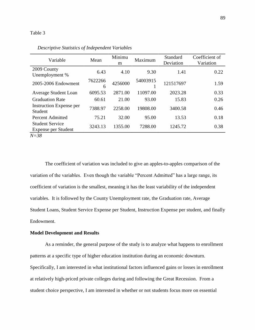
Descriptive Statistics ..............................................................................................86

Model Development and Results ...........................................................................89

Regression Model Estimation ...........................................................................90

First Model ........................................................................................................90

Spending-combined, graduation rate removed .................................................92

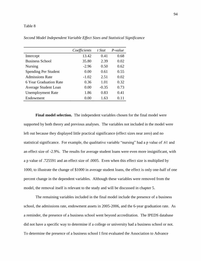
Final Model Selection ......................................................................................94

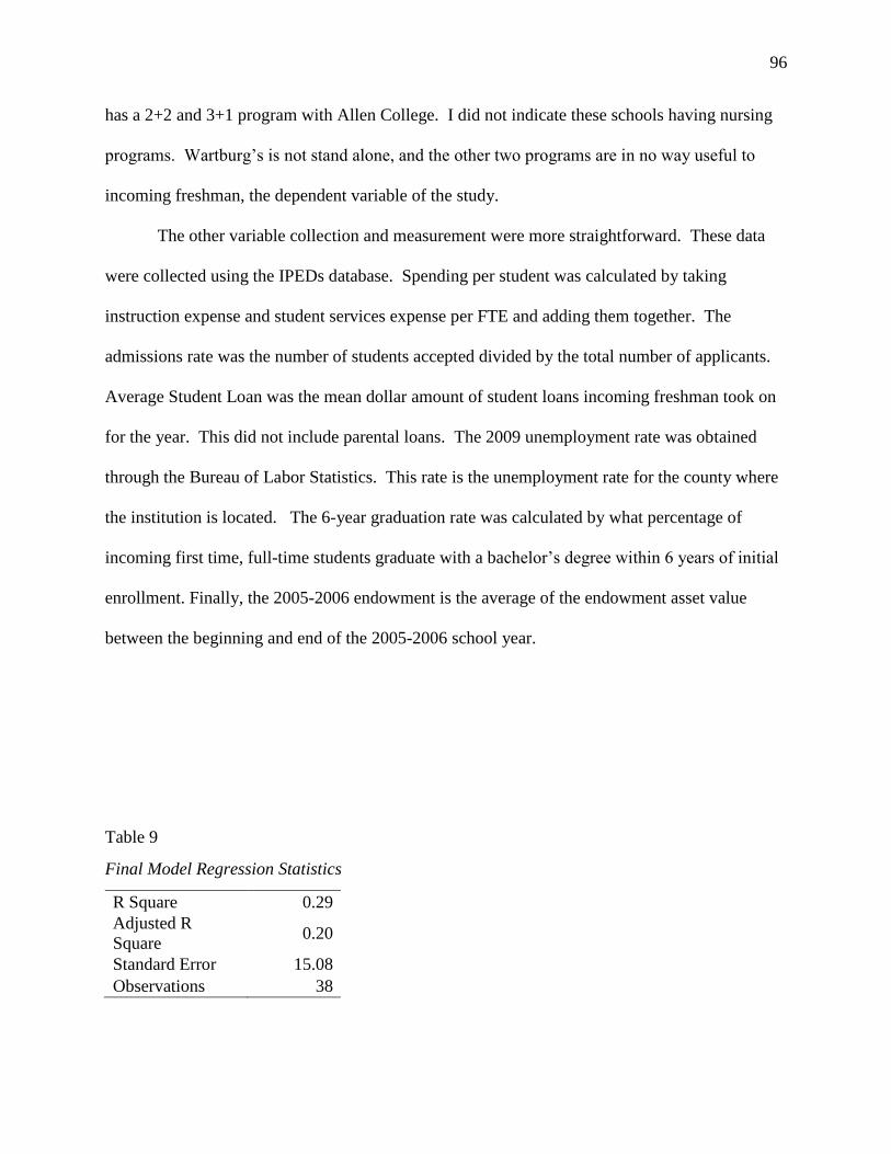
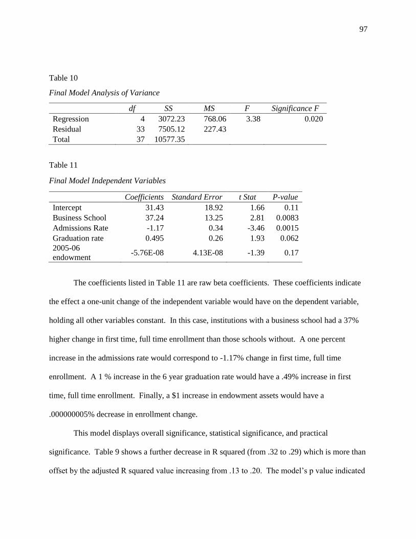
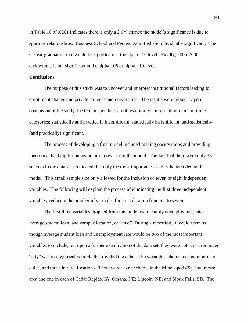
Conclusion .............................................................................................................98

Chapter 5. Conclusions, Implications, and Recommendations ........................................103

Summary of the Study……………………………………………………….....104

Conclusions from the Study .................................................................................105

Prestige Matters ...........................................................................................109

Business Programs Matter ...........................................................................112

Non-Significant Professional Programs .......................................................113

Non-significant, but included variables ..............................................................114

Research Question Revisited ..............................................................................115

Recommendations/Things to Ponder ..................................................................116

Making unpopular decisions in good times ..............................................118

Evaluating Short-Run Tradeoffs ...............................................................118

Limitations and Future Research ........................................................................119

Final Conclusion .................................................................................................121

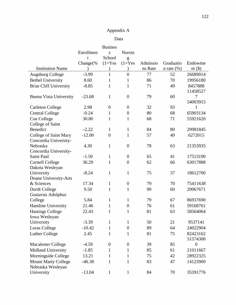
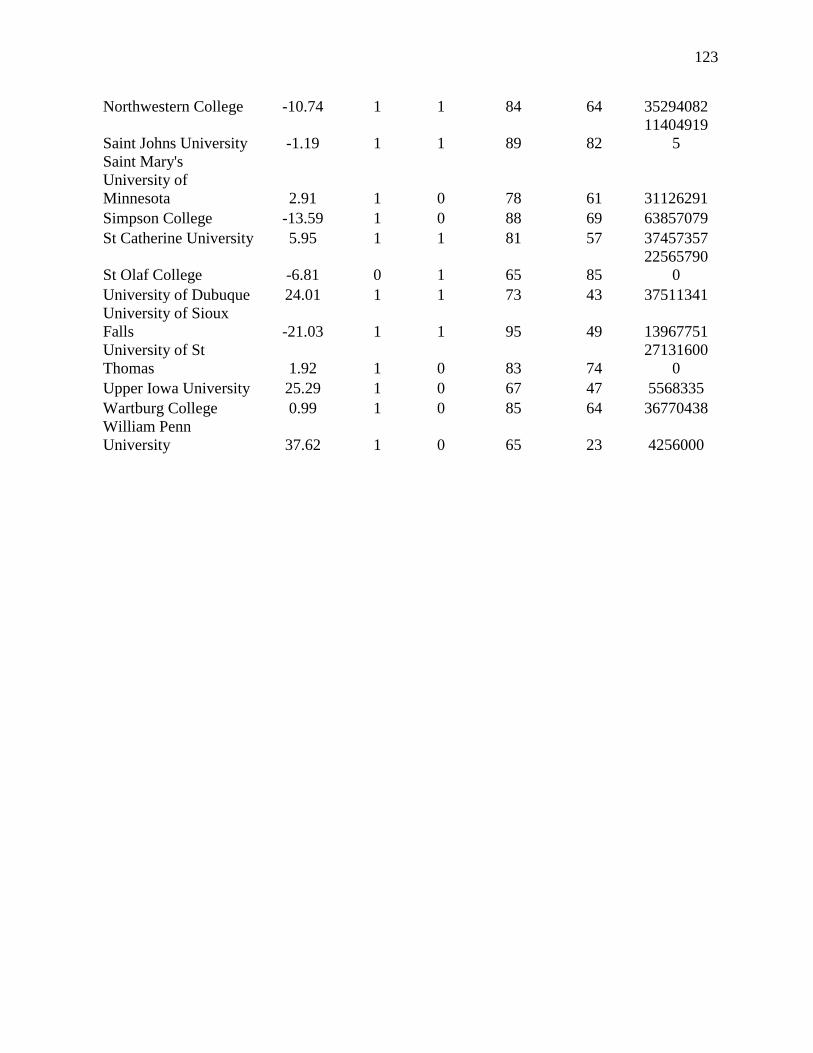
Appendix A……………………………………………………………………………..122

References ........................................................................................................................124

1

CHAPTER 1. INTRODUCTION

From the day I first enrolled in doctoral courses until the conclusion of this study, the

impetus for completion has become more pure in nature. At first, continuing my education

lacked purpose because at the baccalaureate level, formal mastery and training in my discipline

(Economics) beyond the Master’s level was not necessary. In fact, teaching undergraduate level

economics courses did more for me as an economist than any of my seven years of formal

training. In addition to not needing more training as an economist, the coursework was not

possible without quitting my full time job. The real reason I wanted to complete a terminal

degree was because completion was a nearly universal requirement for any career advancement.

Fortunately, the part-time nature of the program and the extended time I took to complete my

dissertation has revealed a greater purpose for completing a doctoral degree.

The concentration (Collateral Component) of my doctoral coursework is higher education

leadership and administration. This program and concentration fits as well as any other

competing program. This “fit” could be described as a relationship of convenience. The core

courses, cohort experience, and research process have developed this relationship into something

much deeper. Whether it is understanding the history of political power and the oppressed, how

good leaders stumble, the source and structure of power, or understanding conceptual

frameworks, the inquiry in the core courses has greatly influenced how I approach research.

Ultimately, this has caused more motivation to succeed in my present-day job and in future

career aspirations.

Currently, I am starting my second year of employment as an Associate Professor of

Practice at a large state institution where there is a large emphasis on research. Prior to this, I

held teaching positions at two smaller universities and a community college for ten years. My

2

current position addresses the secondary nature of undergraduate education as part of the mission

of land grant institutions, especially those with faculty under pressure to publish. Broadly, this

position heightens my awareness of the overall importance of quality undergraduate education.

Personally, the lack of emphasis on teaching at my university has forced me to reflect on the

value of my own private education. This thought experiment, the core education of the program,

my interest in economics, and ultimately a thorough review of literature completed the necessary

force to allow me to complete the study.

As an undergraduate student, I was fortunate that my primary education was excellent, as

was my familial support. Although it is impossible to tell, I believe I would have been

successful at most institutions of higher education. Still, I am always thankful for my decision to

attend a small private institution, despite the higher cost. I believe the small class size and

teaching-focused faculty changed my experience from the status quo to something much greater.

Hardly a day goes by that I am not able to see how my undergraduate education has made me a

better person. I also understand how my experience has a direct impact on family, and my

students as well. Communicating the importance of education, whether to my first grader or a

21 year old in my class, is a daily learning objective.

One outcome of my undergraduate training is the way I view life from the standpoint of

an economist. Specifically, I am intrigued by decisions people make when it comes to scarce

resources. How people utilize their time and money is fascinating to me. From that viewpoint,

the motivation of this study is to understand why students would choose to attend college at an

institution like those in this study when a lower cost option is available during an economic

downturn.

3

As an economist who believes in free markets, I trust market outcomes are indicative of

the highest and best use of scarce economic resources. These resources, generalized into the

categories land, labor, capital, and entrepreneurial skill, are all used in the delivery of

undergraduate higher education. In general, economists believe that if a firm fails, those

resources shall be used elsewhere for a better cause. When markets are efficient, welfare for

society is maximized. This does not mean there are not winners and losers. “Dutch Disease,” is

an economic concept of uncertain origin that describes the secondary effects of positive primary

economic scenarios (Corden, 1984). The general case of Dutch Disease points out the negative

effect on countries after the discovery of a valuable resource such as natural gas or oil. Corden

(1984) summarized much of this literature, and expanded, pointing out that many other factions

of an economy could be adversely affected. The case of higher education dynamics during a

recession is not a direct parallel to Dutch Disease. However, it does provide a premise to

examine the secondary effects of a market disturbance, especially one as large as the Great

Recession.

Believing in market efficiency is a leap of faith. The assumptions of a perfectly

competitive and, therefore efficient market, are as follows: many buyers and sellers, perfect

information, identical product, free entry and exit, and no trade secrets (McEachern, 2011).

Economists have developed models when these assumptions are broken. In the case of higher

education, Oligopolistic Competition fits the market for higher education as the assumptions of

many sellers and identical products are broken (Friedman, 1983). Non-economic literature

supports other deviations from the classical assumptions of perfect competition. Clearly,

students choosing to attend college during high school do not have perfect competition

4

(Simonshon, 2010). Other research on college choice indicates that the economy is playing a

larger role in college choice (Long, 2004).

As mentioned previously, I attended a small private university as an undergrad. I also

attended a public research institution with over 30,000 students to earn my master’s degree.

From there, I taught at my alma mater, followed by a community college, and then a much

smaller public institution trying to gain a higher research profile and now my current position at

a large, public research university. The experience I have as a student and educator gives me a

special perspective on the role of undergraduate education. I am a cheerleader of small colleges,

but above that, I am an economist. If a college or university is to fail due to the efficiencies of

free markets, I want it to be because the outcome is pure and true. I do not want it to be because

stakeholders at those institutions were without the information needed to make necessary

conditions to survive and thrive.

Statement of the Problem

The broad problem this study addresses is access to education. In a 2015 State of the

Union Address, President Obama focused on providing economic prosperity. His first

suggestion was raising the minimum wage, but what was really provocative was his plan to

“upgrade” the skills of future workers through free community college (Obama, 2015). Clearly

education is a direct path to economic prosperity (Hout, 2012). If small private colleges and

universities are spending money on non-academic features to attract students, financially needy

students may not view these institutions as viable options. Access to education is not as simple

as an opportunity for enrollment, it includes geographic access, economic access, programmatic

access, and preparatory access (Windham, Perkins, & Rogers, 2001). If students experience

hurdles to any type of access, enrollment patterns could be affected at several levels of higher

5

education. The displacement of students due to cost could have negative implications for other

students. If these implications have merit, future leaders could use this study’s results as a

resource for decision-making.

More specifically, this study addresses The Great Recession of the past decade and the

corresponding shift in overall consumer behavior as it pertains to higher education. Words like

“austerity” have become mainstream, as has the popularity of conservative personal financial

strategies. During the recession, consumers were seeking value in individual purchases instead

of features, luxury, or non-essential qualities (Bohlen, Carlotti, & Mihas, 2010; Flatters &

Willmott, 2009). Despite this shift in consumer behavior, the cost of attending private colleges

and universities continues to rise. This study aims is to establish a framework for researching

how high-priced producers of higher education (relative to publicly-funded competitors) can

survive a recession and shift in consumer preferences.

Purpose

The purpose of this study is to explore factors that explain enrollment and retention at

small private colleges and universities throughout the Upper Midwest during the Great Recession

that occurred in 2008. This information could be useful for understanding how institutions can

insulate themselves from extreme fluctuations in the business cycle. The existence of these

schools is part of the larger issue of access to higher education in general, which also provides

purpose.

I believe several stakeholders could benefit from this study. The first group is relevant

institutions. The evaluation of private college and university decisions within the framework of

an oligopolistic industry could change decision-making, specifically pertaining to large non-

academic expenditures. In other words, decision-makers could have a more explicit

6

understanding of the internal and external forces driving enrollment decisions. These changes

could lead to better institutional financial health, lower tuition costs, and thriving enrollment.

The student body is a stakeholder as well. Small private schools offer unique qualities that

enhance learning outcomes. If hurdles to access to these institutions are eliminated, many

students could see positive outcomes that would not be associated with other avenues of higher

education. The following question guides the study:

What fixed institutional factors influenced relatively high-priced private colleges to survive

and thrive through the Great Recession?

Procedures/Organization

The organization of this study and the procedures used are that of a traditional five

chapter, quantitative dissertation. My personal and professional background previously

discussed provide the motivation for the study. Chapter Two contains review of literature

supporting a raionale for the research. Chapter Three includes a description of how data were

collected, analyzed, and communicated. Chapters Four presents the results of the study. As an

economist, I am used to overly technical quantitative studies that are only understood by the

researchers and perhaps only a handful of other experts in the area. For this reason, I have tried

to utilize the most straightforward quantitative methods possible. The model used to analyze the

research question was a hedonic model utilizing an ordinary least squares regression. Both

statistically significant and insignificant results provide insight into the proposed research

question. Chapter Five utilizes economic theory and leadership theory to interpret the results in a

richer fashion.

7

Conceptual Framework

The purpose of reviewing established literature in the next chapter is to provide support

for my preconceived beliefs, review how the topic has evolved, and finally provide a space for

where this new study can add to the existing body of literature.

Indeed, the educational outcomes I experienced as a student were not unique. Many

students experience positive outcomes at small private colleges. Despite these positive

outcomes, small private institutions are moving away from a liberal arts tradition to a focus on

applied programs (Jaquette, 2013). The reason for this shift is clear, except for the most

prestigious institutions, maintaining enrollment is key to survival (O’Connel & Perkins, 2003).

The way these institutions compete fits the way firms and organizations in for-profit industries

behave (Jacob, McCall & Stange, 2013). Therefore, the underlying economic theory of firm and

organizational behavior provide a framework for analysis.

On the other hand, the finance and economics of institutions of higher education is

unique (Paul, 2005). To begin, the choice students face when picking a college or university is

very complex (Chapman, 1981). Three areas of the literature review narrowed the focus of the

study. These areas are college choice, the theory of luxury goods, and the effect of a recession

on firms selling luxury goods during a recession. The Great Recession was a once in a lifetime

economic downturn, and the shift in consumer attitudes was real and pronounced (Flatters

&Willmott, 2009), but the dynamics of the recession were not limited to the demand side. From

the viewpoint of colleges and universities (the supply side), the constant pursuit of prestige and

how this pursuit affects stakeholders is relevant. My study aims to address both.

8

Definition of Key Terms

Game Theory: The study of strategic behavior (Friedman, 1983).

Hedonic Model: A multiple regression model utilizing characteristics of a heterogeneous product

to explain variation in product price (Studenmund, 2001).

Luxury Good: A good or service highly responsive to change in consumer income (Besley,

1989).

Oligopoly: A market in which there are only a few firms and all firms are interdependent

(Friedman, 1983).

Product Differentiation: Changing a product in such a way that consumers can discern

differences between competing products (Friedman, 1983).

9

CHAPTER 2. REVIEW OF LITERATURE

The goal of this study is to explore factors that explain enrollment and retention at small

private colleges and universities throughout the Upper Midwest during the Great Recession. The

small private colleges of interest for this study are what have been commonly referred to as

“liberal arts schools,” typically with small residential campuses. To understand the competitive

environment of small, private institutions, it is important to understand issues related to prestige

and inclusivity. This literature review is divided into these nine sections: small private college

or university education; the finance and economics of higher education; economic theory;

prestige; inclusivity and access; the Great Recession; luxury goods; college choice; and

marketing. Following the topical literature review is a conclusion revealing the emerging themes

and trends to support this study.

Small Private College or University Education

One of the foundations of this study is that education in a small setting has some

advantages over the educational experience provided by larger public universities, community

colleges, or online programs. In a modern, but not contemporary essay, McPherson and

Schapiro (1999) recounted President James A. Garfield’s version of an ideal education.

President Garfield believed the best setting for college and/or learning would be himself at one

end of the log and the president and professor of his alma mater at the other end for the purpose

of emphasizing the importance of low student/faculty ratio and the importance of teaching at a

university. The essay concluded with a rationale for the continuation of the liberal arts

educational tradition, noting, “The residential liberal arts college, at its best, remains almost a

unique embodiment of a certain ideal of educational excellence” (p. 73). While the article

focused on liberal arts, it is also clear that mission, size, and faculty are key components of their

10

educational Shangri-La. The authors asserted that if the definition of a liberal arts school is

strictly adhered to, the number of true liberal arts colleges is very low as many are focusing on

more applied and professional programs. This is not a negative outcome as it is clearly displayed

there are many pseudo-liberal arts institutions that can offer the same benefits to students through

the focus on one main quality: faculty-student interaction (McPherson & Schapiro, 1999).

From a similar standpoint, Williams College trustee Paul Neely wrote about

contemporary threats to liberal arts colleges (1999). Neely, a newspaper publisher by trade,

makes compelling statements about the competition soon to challenge liberal arts colleges. For

example, the University of Arkansas, once thought to be a lower-tier school, is now a legitimate

threat to smaller, more highly academically regarded institutions. Juxtaposing the University of

Arkansas is Williams College, which has a sterling reputation and national prominence. Neely

used Arkansas as an example of emerging competition to Williams, but noted other public

universities, community colleges, and online universities as potential threats to the upper crust,

elite private colleges (1999). Neely’s article is not necessarily a pessimistic view of liberal arts

education. Instead, it is a practical evaluation of the changing world of higher education.

Neely’s anecdotal observations from the boardroom about competition illustrate almost all the

current issues faced specifically by liberal arts colleges, most of which can be applied to any

small private institution.

While searching for, and reviewing the literature related to the topic of this study, it

became clear the imprecise use of terminology would become problematic. Taylor and

Morphew (2010) noted, “Small, 4-year private colleges are commonly referred to as ‘liberal arts

colleges’ in the United States. Many times, however, this label is applied inappropriately” (p.

484). Breneman defined liberal arts schools as those that met the following criteria: grant greater

11

than 40% of their degrees in traditional liberal arts fields, have less than 2500 students, are

largely residential, and have a student body of traditional age (1994). Even with a specific

definition, the goals and purposes of a liberal arts college can be applied to schools that are

technically not liberal arts colleges (Taylor & Morphew, 2010). Neely wrote, “At many of the

hundreds of schools that call themselves liberal arts colleges, the term represents nostalgia more

than curriculum” (1999, p. 36). To avoid confusion, this study will categorize schools by size

and campus type. While the academic profiles of these schools can vary, this study aims to

evaluate traditional baccalaureate schools with face-to-face delivery and some type of on-campus

housing.

Carnegie classifies schools by degree type and size as sub-classifications. By size, two

categories are relevant, VS4 and S4, indicating fewer than 1000 students (VS4) and under 3000

students (S4). Also of relevance is the type of campus. Carnegie has classifications for the

residential makeup of the institution. The only schools excluded from consideration in this study

are those with fewer than 25% of students living on campus. This information is provided by the

newer, more sophisticated Carnegie system and database. It should be noted the colleges and

universities in this study are private and not explicitly funded by the state in which the college or

university resides. For example, the university branches that make up the University of

Wisconsin system would largely be included if not prohibited by their public funding.

On the topic of selectivity and rankings Ehrenberg, a researcher at the Cornell Higher

Education Research Institute, pointed out that selectivity and rankings are becoming increasingly

complex (2005). In addition to the complexities of the US News and World Report (USNWR)

rankings, Ehrenberg pointed out it is possible and likely that institutions are able to easily

manipulate their USNWR ranking, specifically with respect to selectivity (2005). One way an

12

institution can enhance selectivity is by rejecting qualified applicants if it is unlikely the

applicant would enroll if accepted (Ehrenberg, 2005). This practice has no rationale other than

enhancing ranking, and actually causes other negative distortions (Ehrenberg, 2005). Barron’s

Profile of American Colleges, a former standard in college ranking guides, uses only four broad

levels to rank selectivity, based only on entrance exam scores (Ehrenberg, 2005). While the

simplicity of this approach could be useful, Ehrenberg pointed out that no ranking within strata is

defined (2005). Multiple authors use the USNWR guide as an official ranking, and it appears it

has become the preeminent ranking guideline in general. Ehrenberg warned this is only because

the USNWR rankings look scientific because of the use of a very complex formula; in actuality

the ranking is not as unbiased or “academic” as it would appear (2005).

Selectivity appears to be a sub-issue of how the market for college enrollment has

recently changed. It would seem logical that a population growing faster than the number of

colleges would increase selectivity, and anecdotes support this logic, but Stanford Economist

Hoxby turned this idea on its head. She argued that if all other things remained the same, this

logic would be correct, however, something did change, and that is student mobility. She

asserted that the old model of going to a college or university near one’s hometown is simply out

of date. Students understand the benefits of finding the school that suits them best, and colleges

and universities understand their effective monopoly is no more. When this is combined with

lower costs of travel (both implicit and explicit) and the availability of information, the number

of institutions of higher education a student will consider increases (Hoxby, 2009). Perhaps the

most notable outcome of mobility, according to Hoxby, is that selectivity overall is decreasing.

Only the top ten percent of higher educational institutions have experienced an increase in

selectivity over the past 50 years. Mobility is the main reason for this change because colleges

13

and universities can no longer operate what is in effect a regional monopoly. If students do not

gain entry to their regional college of choice, they are able and willing to attend elsewhere. This

decrease in selectivity for all but the top tier institutions of higher education is one symptom of

the emerging dichotomy in selectivity amongst institutions of higher education in the United

States: schools are either selective, or they are not (Hoxby, 2009).

Small private college and university outcomes. In a study on the effects of a liberal

education, Seifert, Pascarella, Goodman, Salisbury, and Blaich used the definition of a liberal

arts institution previously used by The Center of Inquiry in the Liberal Arts for their research

(2010). The definition is divided into three parts: (a) the pursuit of intellectual knowledge and

critical thinking, (b) an interrelated learning environment where everything institutionally related

connects, and (c) a focus on student-faculty learning relationships (as cited in Siefert et al.,

2010). This definition, although similar to the previous definitions of a liberal arts institution,

has a greater focus on mission.

Jaquette (2013) related the mission and/or changing mission of colleges and universities

to the enrollment economy, stating that mission drift is in response to the demands of students,

parents of students, and employers, all looking for definitive and immediate measureable results

from higher education. Finally, the definition of college versus university shows up in the

previously mentioned literature on college rankings (Hoxby, 2009).

What is similar in all of the literature about private liberal arts education is size and

student engagement. Certainly there is wiggle room in the definition of what is or is not a liberal

arts institution. However, there is little ambiguity with regards to the size of a university.

Whether the educational focus is liberal arts or more applied, a lower faculty/student ratio

14

indicates an emphasis on student learning giving impetus to research and explore schools such as

those in this study.

The Finance and Economics of Higher Education

Because this study takes aim at an issue from an economic standpoint, it is important to

discern the difference between the terms economics and finance as they relate to the topic. In

discussing finance, I am referring to the hard facts about the business of higher education, which

include the cost of attendance, tuition rates, trends, and other factual information. Economics

refers to a discussion of higher education within the context of economic theory and competition.

Finance

One always-present issue is with the rising cost of college. Nearly every article I

reviewed indicates that the cost of college attendance is advancing at an extraordinary rate.

Often superlatives are used to describe this trend, but beyond this dramatization, authors agree on

little. For example, some authors seem to provide support for both sides of the argument about

the true expense of college; at the very least their statements are not one-sided. Karikari and

Dezhbakhsh, (2013) stated that public college tuition has increased at a faster rate in percentage

terms (3.5% vs. 5.1%) than private tuition from 1995-2004. Later in the same article it is

revealed the absolute change in tuition is still considerably greater at private colleges and

universities, approximately $7,000 vs. $4,000 at public universities. Continuing this

inconsistency, Slaper and Foston (2013) wrote an article titled, “Onward and Upward with the

Cost of College,” but then cited a Wall Street Journal Article (as cited in Slaper and Foston,

2013) revealing the increase in tuition in 2013-2014 to be the smallest in 12 years. This is

certainly not an expected statement given the title. Although the discussion about price is

confusing, it is for good reason and an example of how even the smallest details confuse the

15

topic. For example, Foston (2013) explained the semantic difference between the words “cost”

and “price.” This example is subtle, but the message is clear: prices and costs are going up, and

beyond that assertion, little else is obvious (Foston, 2013).

In a study driven by economic theory, Buss, Parker and Rivenburg (2004) attempted to

model enrollment demand at small institutions of higher education. Their model is very

straightforward. The researchers hypothesize that price, discount rate, price of substitutes,

income, and prestige would be strong predictors of enrollment. The authors split students into

two groups, those with and without financial aid. While there were some minor differences

between the two groups, the overall takeaway from the study was that tuition was by far the

number one driver of enrollment (2004). This work is also relevant to the model of this study,

which will be explained in detail later.

The literature about the high cost of education reveals the reasons for tuition differentials

between publicly funded and privately funded institutions of higher education. At public

universities, the increase in tuition is due to decreases in state support, which is then simply

backfilled through reducing expenditure per student and raising tuition (Martindale, 2015).

Private universities, on the other hand, have been forced to increase tuition because of increases

in expenditure per student, mainly in the form of non-academic programs. This includes things

like housing, food, facilities, varsity sports, and many other services (Ehrenberg, 2012).

The outlook for future tuition costs consistently indicates the upward trend will continue,

but the reasons vary. Recently, Wight Martindale Jr., an adjunct professor at Villanova and

former finance editor of Business Week, asserted that tuition is expensive and will stay expensive

(2015). Martindale noted four reasons why the cost of attending college will remain high: (a)

there are a limited number of institutions, (b) colleges and universities are getting fancier, (c) the

16

experience is fun, and (d) there is an increased attraction from students abroad (2015). While

Martindale’s demand-side analysis looked forward, Foston (2013) looked back and concluded

that internal and external cost (supply) drivers are to blame for rising costs. There is no evidence

in either article, however, that the causes are mutually exclusive. This would indicate there is no

reason that both supply and demand drivers could not assert influence simultaneously. There is a

substantial amount of literature using supply-side factors to explain the increase in the price and

cost of higher education. Conversely, there is far less literature and discussion trying to reveal

demand-side reasons for rising prices and costs (Jacob, McCall, & Stange, 2013).

Economics

The financial state of higher education sets the stage for the economics of higher

education. As Paul (2005) pointed out, the university “is also a complex business with a range of

intertwined functions and responsibilities that come together to create educational products and

services” (p. 107). While most universities are not-for-profit unlike traditional economic firms,

the production of services and need to maintain financial health warrants an economic

explanation of behavior. Like for-profit firms, a main goal of a not-for-profit is continued

existence, which obviously depends on the pursuit of positive financial and economic outcomes.

The analysis of firm behavior is central to microeconomics. The formal definition of

microeconomics, “the branch of economics that analyzes the market behavior of individual

consumers and firms in an attempt to understand the decision-making process of firms and

households,” (Pindyck & Rubinfeld, 2011, p. 4) sets up a discussion of how both producers

(colleges and universities) and consumers (prospective students) make decisions regarding

higher education. Before considering these decisions from either perspective it is important to

understand how complex the economic analysis is for two distinct reasons. First, the consumers

17

(students) are an input in production of the service. Second, the college choice/enrollment

decision lacks information on both ends. Fortunately, there is research to explain the unique

consumer input scenario at colleges and universities.

Economics at prestigious institutions. O’Connell and Perkins (2003) explained the

economics at private liberal arts colleges, asserting that competition for students means two

different things depending on prestige and enrollment status. Colleges and universities that have

prestige and the name recognition and endowments that come along with it typically set tuition

prices strategically low. This low price ensures a shortage and, therefore, the ability to select

only the best students. In this case, the shortage refers to admission. These colleges and

universities have more applicants than their capacity; therefore, there are consistently more

people willing to pay for admission than possible. These high-achieving students then act as

inputs, effectively teaching the very classes they are enrolled. O’Connell and Perkins (2003)

noted this creates a feedback loop: good students teach other, which saves costs. The students

graduate, become successful, and give money back to their alma mater, thus giving the

institution the continued ability to keep tuition below the market price and furthering the ability

to select the best students.

This does not mean prestigious colleges and universities are giving away their product,

tuition prices at these institutions are only “low” in the economic sense as the price charged is

not as high as they could charge and still maintain full-enrollment. One side effect of below-

market pricing is that due to increased mobility (Hoxby, 2009), the “low” price selective colleges

charge actually becomes more expensive to lower-income families when compared to their

income (Dezhbakhsh & Karikari, 2010). It would not be hard to imagine that schools like

18

Harvard and Yale could charge double or triple their current price and still fill up seats. A “low”

price is clearly relative.

Economics at non-prestigious institutions. Competition for students at colleges and

universities without high levels of prestige does not maintain the complex input/output scenario

as described at prestigious institutions. Instead these colleges and universities rely on student

enrollment and tuition as a main source of revenue and not as an input in the production of

education (O’Connell & Perkins, 2003). O’Connell and Perkins compared the situation of

prestigious institutions with the tough situation faced by institutions without prestige. Colleges

and universities without prestige seek prestige, but the only way to do so is by spending money

on academics (2003). Unfortunately, their short-run goals are to make ends meet, which

predicates attracting students by whatever means necessary. These strategies typically do not

include spending money on academics, the only way to gain prestige (O’Connell & Perkins,

2003). While O’Connell and Perkins specifically cited a feedback loop for prestigious

institutions, it seems as though a similar but negative pattern emerges for colleges and

universities without prestige. If this is the case, the difference between institutions of higher

education with prestige and those without would become even greater.

As my review of the literature on the finance, education, or competition of higher

education has evolved, it has become increasingly clear how complex the topic is. The literature

is thin on one issue, a demand-side analysis of consumer preferences and subsequently one of

institutional behavior (Jacob, McCall, & Stange, 2013). In an article addressing how

consumption patterns of college students have changed over time, Jacob, McCall and Stange

legitimized the headlines of popular periodicals noting the changing role of consumptive luxuries

in student choice and enrollment (2013). In other words, college is becoming more like a

19

country club than what most of us remember. For the purpose of this study, two quotes from the

Jacob, McCall, and Stange (2013) stand out: “Less selective (but expensive) schools, by

comparison, have a greater incentive to focus on consumptive amenities” (p. 4) and, “In fact, our

estimates suggest that relatively few students actually place a positive value on instructional

spending” (p. 26). On the other hand, Jacob, McCall and Stange asserted that spending on

academics will result in the increased enrollment of high-achieving students; however, they

noted this will most likely inhibit the institution’s ability to attract other students (2013). These

quotes support the educational purpose for my study; non-selective schools are choosing short

run enrollment success due to students’ demand for consumptive luxuries over long run success

and better educational outcomes.

Product differentiation. Competition for students also relies on whether or not colleges

and universities can actually differentiate themselves. The premise of a monopolistically

competitive or oligopolistic industry, which most closely resembles the industry of higher

education, is that individual firms are able to set themselves apart from other competitors. This

study looks at one specific market, small institutions of higher education, within the much larger

overall industry of higher education. Neely (1999) pointed out the likelihood that pressure from

exogenous forces could actually be commodifying higher education. Brint, Riddle, Turk-

Bicakci, and Levy (2005) discussed curricular changes at all institutions of higher education,

noting the shift seems to be away from a liberal arts focus to one of practical training. Students

at non-prestigious colleges and universities are driven by career-oriented goals, making the need

for a high-priced liberal education less attractive (Brint et al., 2005). Neely (1999) feared that

students enrolled at prestigious colleges and universities for their undergraduate education will

pursue graduate degrees at higher rates at large research universities, turning small private

20

colleges and universities into high-priced prep schools that will become extinct exactly as

passenger trains did in the mid-20th century. Again, Neely was not negative about the

effectiveness of private colleges and universities, he simply was speculating a potentially

negative outcome.

This does not mean that colleges and universities do not or cannot differentiate

themselves. Two areas where institutions of higher education can differentiate themselves are

size and quality of education. Koshal and Koshal (2000) studied whether colleges and

universities experience economies of scale and/or scope and how a quality variable could be

utilized. Their study began with the example of Swarthmore College and Williams College

juxtaposed against Hannibal-Lagrange College as a premise for identifying a quality variable

(2000). While economists may be guilty of assuming too much, Koshal and Koshal’s

assumption is backed by specific research. There is specific evidence that the overall quality of

education can be both improved, and that the improvement can be quantified (2000). Koshal and

Koshal collected data on 295 of the 500 liberal arts colleges in the United States (2000, p. 212).

Their main assertions were that institutions smaller than 2343 students could benefit from

growing (2000, p. 219). The other main finding pertinent to this research is that while

economies of scope exist by offering graduate education, research is not cost-effective at small

institutions of higher education (Koshal & Koshal, 2000)

Other literature discusses how colleges differentiate themselves in different and more

tangible ways. Arizona State University (ASU), one of the largest public institutions in the

country, seems to understand the fruitless pursuit of becoming the next Ivy League or Berkeley-

quality institution. ASU is utilizing other strategies to augment their internal and external

success (Crow, 2010). Crow, the President of ASU at the time, wrote about delivering authentic

21

educational experiences while still maintaining the inclusivity that allowed ASU to have

unprecedented enrollment success (2010). While size may affect how institutions of higher

education achieve goals and outcomes, the goals and outcomes do not seem to differ between

large, small, public, private, selective, or non-selective institutions. Crow stated that ASU is a

giant public university, yet it aimed to deliver the same outcomes as small, private institutions.

The words of ASU’s president about ASU obviously show some bias, but are echoed

elsewhere. There is an argument that once an institution is inclusive, meaning it has the ability

to accept and place all applicants, the value of a college degree decreases (Covaleskie, 2014), or

that universal access is little more than trade school (Trow, 2007). While this paints a negative

view on the economic and/or monetary aspirations of college goers, it does suggest that once all

have economic gains, the truest gain of education can be redeveloped, much in the way Crow

(2010) envisioned the mission/vision of Arizona State University. Even if a college degree loses

economic value because the supply is too great, the non-monetary outcomes of higher education

will be numerous and in line with the traditional learning outcomes associated with higher

education.

Most of the articles reviewed for this study examine liberal arts education, private

education, and small residential education as well as provide evidence to support positive

outcomes. Seifert, Pascarella, Goodman, Salisbury, and Blaich (2010) compared the outcomes

of small liberal arts colleges and universities against Chickering and Gamson’s (1987) seven

principles of good practice in undergraduate education. Of the seven principles, small liberal arts

colleges and universities had an advantage over larger institutions in the following categories:

good teaching, high quality interactions with faculty, academic challenge, and high expectations

(Seifert et al., 2010). Interestingly, Seifert et al. also discovered similar positive outcomes at

22

community colleges. The community college outcome initially looks like evidence against the

worth of a higher priced educational experience. However, the researchers make it clear the

positive outcomes are for different reasons. Community colleges offer better outcomes than

large research institutions because of higher levels of structure and support for lower-achieving

students while small liberal arts colleges and universities provide positive outcomes for all levels

of students (Seifert et al., 2010). The researchers identify funding as the main variable to explain

differences in advising experiences and the outcomes between community colleges, small private

institutions, and large public institutions of higher education. Schudde and Rab (2014) also

believe that community colleges are effective at academic advising, but lack the monetary base

necessary to counsel students in non-academic areas.

Economies of scale. For colleges and universities without high levels of prestige,

competition not only comes from other similar institutions, but from online institutions as well

(Burrell, 2008). Whether competing against online programs or each other, bottom tier private

colleges are in competition for enrollment (O’Connell & Perkins, 2003). The most pragmatic

purpose behind attracting more students for these institutions is economies of scale, the idea that

increasing output (in this case enrollment) lowers the per-unit cost of production. Minimum

efficient scale is the size of production that minimizes per unit cost. According to the research of

O’Connell & Perkins (2003), the minimum enrollment for small liberal arts colleges and

universities is somewhere between 1500 and 2000 students. Koshal and Koshal (2000) identified

2,343 students as the ideal number of undergraduates for taking advantage of the cost savings

associated with adding students.

It is clear that small private colleges not at capacity, or below the 1500-2343 student cost

minimizing standard (Koshal & Koshal, 2000; O’Connell & Perkins, 2003), are interested in

23

increasing enrollment to take advantage of economies of scale. The literature tells two stories

about how this is achieved. The pragmatic approach, advertising outcomes, may actually have

an adverse effect on future reputation. Ehrenberg (2012) described the information asymmetry

between buyer and seller in this scenario. For marginal students the asymmetry is that they do

not understand why they should attend any specific college. To increase enrollment, colleges

and universities diversify and tout more applied programs. On the non-academic side they

promote student service expenditures, or other non-academic programming to increase student

interest (Ehrenberg, 2012).

By focusing on enrolling marginal students by way of non-academic recruiting, these

colleges risk long run success. “Reducing the cost of college will involve gut-wrenching anger-

inducing trade-offs” (Foston, 2013, p. 8). These tradeoffs could be short-term enrollment

success versus the overall long-run health and viability of the institution (Foston, 2013; Jacob,

McCall, & Stange, 2013). While current competition for students is fierce, the long run growth

model includes raising the reputation of the college or university, which can be done by investing

in academics and is only successful if high-quality students enroll (O’Connell & Perkins, 2003).

Enrolling marginal students does not fit the long run growth encouraged by any of these

researchers.

Market price and discount. The biggest difference between a perfectly competitive

market and higher education is the assumption of price-taking behavior, which O’Connell and

Perkins (2003) suggested is the market for higher education. This difference is apparent when

analyzing the financial trends in higher education. While tuition has gone up, so too has the

discount rate (Ehrenberg, 2005), which also increases the ability to discriminate students’

willingness to pay. By doing this, institutions are able to charge a unique price to each

24

individual student. The colleges and universities offering a high discount rate (Ehrenberg, 2005)

match those O’Connell and Perkins (2003) described as having a lack of prestige. Simply put,

the institutions without prestige and, therefore, financially dependent on enrollment, are likely to

be the ones heavily discounting tuition as Ehrenberg (2005) described. Institutions of higher

education competing for students as revenue drivers and not as production inputs will

individually lower prices to put bodies in seats and beds. From an economic standpoint, price

discrimination and discounting allows non-prestigious colleges and universities to maximize

revenue, a response to a surplus of product, which reinforces the non-selective and non-

prestigious nature of the institution.

The ability to set a price below equilibrium and to not discount tuition to attract students

allows selective institutions to be just that—selective (O’Connell & Perkins, 2003). This

selectivity can be viewed as a result of two prices: the price selective colleges pay for the input

of student production and the price the student pays for education (Winston & Zimmerman,

2004). Colleges and universities that have the ability to fill classrooms with only high-quality

students can use this as a cost saving measure. Winston and Zimmerman (2004) said that is why

nationally recognizable institutions of higher education, such as Harvard, are able to get away

with graduate teaching assistants teaching large classes as the main instructors. In general, the

students can teach themselves.

Peer effects. Winston and Zimmerman used the phenomenon of peer effects in a

production economics framework to explain that the effect is strong, extensive, and applicable in

many settings/scenarios (2004). Most importantly, these effects can explain why certain markets

in higher education appear to be out of equilibrium. Using high-quality students as a cost saving

measure begets the ability to enhance financial stability in the future. If the reputation of a

25

higher education institution can only be built through its students (O’Connell & Perkins, 2003),

good students are an input in the production of positive education outcomes (Winston &

Zimmerman, 2004), and positive education outcomes result in students making more money

(Martindale, 2015), these students can give more to the very universities that made them who

they are (Winston & Zimmerman, 2004). This is the very reason why less selective colleges and

universities desire to gain the prestige that selective institutions possess.

Prestige

Much of the literature regarding the competition among colleges and universities refers to

prestige as something that is measureable and real; however, the specific prestige each researcher

focuses is without explicit definition. Therefore, this section is devoted to giving an overview of

prestige from multiple viewpoints from the overall university to the faculty and staff, and finally

the students. Finally, this section provides a definition of prestige as it is used for the remainder

of the study.

One way to interpret prestige would be by ranking of traditional outside publications.

Volkwein and Sweitzer (2006) conducted a study to test the validity of the USNWR prestige

rankings. They examined the correlation between the selectivity rankings in the USNWR and

four other common college guidebooks. The correlation between the ratings of other

guidebooks; Barron’s, Peterson’s, Fiske, and the Princeton Review, range from .69 to .83,

indicating a substantial amount of agreement between the four other less-known rating entities.

Although the guidebooks tend to agree on prestige, the researchers aimed to explain what

characteristics of colleges and universities contribute to prestige. The model Volkwein and

Sweitzer finalize in pursuit of explaining variations in prestige had an adjusted R squared of .88.

While this cannot be directly compared to the correlation coefficient between the guidebooks, the

26

model seems to have more explanatory power than the guidebooks. The model, a blocked set-

wise regression, explains prestige using entering SAT, professor salary, faculty productivity,

student-faculty ratio, age of institution, total enrollment, and percent of full time faculty as

significant variables. While all seven variables were statistically significant, the top three

variables have considerably larger effect sizes than the rest, these were SAT, professor salary,

and total enrollment (2006).

As noted previously, the topic of prestige is complex. What is not complex is the nearly

universal pursuit of prestige by all types of institutions of higher education. Toma (2009)

conducted a qualitative study of 38 institutions in the Atlanta area to study prestige at all types of

institutions of higher education in the United States to see how the pursuit of prestige varied at

institutions with varying levels of academic notoriety. Along with his campus observations, he

interviewed 10 upper level administrators at four universities representing four different types of

institutions. The four types of institutions, community colleges, liberal arts colleges,

comprehensive colleges, and large state research universities, all seek to enhance the image and

function of the university, typically striving to be associated with the group of schools seen as

one level superior. The conclusion from the study is that all four types of institutions of higher

education are trying to achieve objectives in the same way, typically, by attracting better students

and faculty and making campus improvements (Toma, 2009). While other authors (Chabotar,

2010; Ehreneberg, 2012; O’Connell & Perkins, 2003; Slaper & Foston, 2013) viewed increasing

costs as a bad thing, Toma viewed this race to the top as something positive. He ignored rising

costs and instead focused on the positive enhancements all institutions make to try to achieve the

prestige of the next level (2009).

27

In a study about the effect of prestige-seeking behavior from the perspective of graduate

education at mid-level doctoral granting institutions, Gardner (2010) found the pursuit of

prestige to have both positive and negative attributes. As Toma (2009) pointed out, the pursuit

of higher levels of prestige increased both the quality of the students and faculty. From the

faculty perspective, increases in funding were obvious positive outcomes of prestige-seeking

behavior. Conversely, the negative side effects of prestige-seeking behavior were the increasing

stratification and negative cultural aspects of graduate education, such as competitive behavior

and high rates of turnover (Gardner, 2010).

Finally, in the most appropriate setting related to the topic for this study, O’Meara and

Bloomgarden (2011) conducted a case study to interpret faculty impact of prestige-seeking at a

high quality liberal arts college which was striving to become nationally elite. In this setting the

results were clear. While there were a few comments about the benefits younger faculty may

enjoy, the consensus was that the teaching mission of the university would be harmed at the

expense of an increased focus on new faculty scholarship and research needed to elevate the

profile of the college or university (O’Meara & Bloomgarden, 2011).

Student applications. From students’ perspectives, prestige is about the value of

education. For some, prestige comes from simply completing a degree, for example, a degree

from an Ivy League school. From the standpoint of gaining admittance to selective institutions,

the trends in higher education create some interesting secondary outcomes. Prestigious colleges

and universities are not expanding in capacity, but applicants are, meaning that fewer and fewer

students are admitted into their first-choice institutions (Bound, Hershbein, & Long, 2009).

Bound et al. outlined the trickle-down effect that this increasing selectivity creates by explaining

how students prepare to compete for college admission (2009). Within an economic framework,

28

the competition between buyer and seller oftentimes relates to the information to which each side

is privy. USNWR seems to level this playing field according to Bound et al. (2009), who pointed

out that this heightened transparency incentivizes students to game the admissions process by

focusing on test scores (AP/ACT/SAT) and other activities. They conclude the end result is

students who have memorized factual content but are not prepared to obtain a true education.

Although not specifically stated, the tenor of Bound et al.’s work is that of negativity. The

researchers opine the process of the admissions game has taken away from the true purpose of

higher education even for those students with the highest level of pre-college achievement

(Bound et al., 2009).

The takeaway from the literature is quite evident; prestige matters. However, a definition

of prestige is hard to come by. In some cases, like Volkwein and Sweitzer (2006), prestige,

selectivity and reputation are used synonymously. For others like O’Meara and Bloomgarden

(2011), prestige can manifest itself in other areas such as research. Even early researchers

confuse these terms as evidenced by Trusheim and Course’s (1981) assertion that “A man’s

occupational status depends greatly on having attended college (Jenchks et al., 1979), but

apparently not very much on the social prestige or selectivity of the college he attends” (p. 296).

Because this study focuses on enrollment trends for institutions financially dependent on tuition

dollars, the adopted definition of prestige shall be, “the ability to turn away qualified applicants.”

Inclusivity and Access

Community colleges provide an easy access point to higher education. Most have few or

no admissions standards and the cost of attendance is explicitly low. In general, having an open

door policy is shown to have overall positive results for both individuals and society at large

(Everett, 2015). While this does create nearly universal access (Trow, 2007), it also can create a

29

negative signal to employers. While a two-year degree is better than no degree, it sometimes

suggests an inferior education (Schudde & Goldrick-Rab, 2014). On the other hand, a two-year

degree can be used as a springboard to a four-year degree or vocational training that has both

economic and non-economic gains (Schudde & Rab, 2014).

Prestige is not something that is binary in nature, even the most inclusive colleges and

universities, such as community colleges, offer some level of prestige. Sociological researchers

Schudde and Goldrick-Rab (2014) examined stratification of higher education with a specific

emphasis on community colleges, through which the United States has emerged as a world

leader in access to higher education (Trow, 2005). Schudde and Goldrick-Rab concluded

community colleges enhance access, but create more stratification and income/social inequality

depending on the student or the situation (2014).

The contemporary discussion of the role of the community college is a good starting

place to reflect on the history of access to education in the United States. The following section

includes a history of access, followed by the history of government intervention and the implied

belief that access to higher education is part of the American dream, especially since the end of

World War II.

Historical access. The assumptions of this study seem to be in line with the assumptions

about higher education made in the past. The primary assumption of research on education is

that going to college is universally a good thing. The research on the benefits of higher

education highlight the benefits to the individual, or the benefits to society. Other than the

explicit opportunity cost of going to college (foregone wages), little harm is ever discussed. That

being said, the benefits of education have not always been as widely accepted, especially when

reviewing the history of higher education from the beginning.

30

According to Longstaff (2014), going as far back as Socrates/Plato/Aristotle, the benefits,

purpose, and right to education exhibit a cyclical pattern. The earliest universities had no

physical location and were available to all. The only prerequisite to attendance was a desire to

learn and understand. Only when the infrastructure of brick and mortar necessitated charging

fees did higher education become increasingly exclusive. Longstaff pointed out the cycle would

be inclusivity followed by exclusivity (2014). Examples of this trend include correspondence

courses in the 19th century (inclusive), low rates of attendance and graduation in the 20th century

(exclusive), and finally the inclusive development of massive open online courses in the 21st

century (Longstaff, 2014).

The exclusivity of college has not always correlated with the economic value of

education. Labaree (as cited in Covaleskie, 2014) pointed this out by noting that obtaining a

degree was a signal of educational attainment and not a signal of economic worth in the past.

Education beyond a basic level was indeed for the upper crust, but the reasons to attend college

historically have not been economic. More simply, until modern times, college attendees would

have economic success waiting in adulthood despite their level of educational attainment

(Labaree, 1999, as cited in Covaleskie, 2014).

After the GI bill and then the Higher Education act of 1965, the trend that a college

education was a right changed to a view of it becoming a cultural belief (Burrell, 1967, as cited

in Bound & Turner, 2002). In either case, the goal of educating the workforce was achieved.

The secondary effect of this legislation was the cultural belief that having access and choice to

post-secondary education was a right. Since then, obtaining a college degree is increasingly seen

as a necessity (Covaleskie, 2014). While this puts pressure on students to attend college despite

what may be their true aspirations, this belief does point to an increasing level of access and

31

inclusivity; whether permanent or as part of the inclusivity/exclusivity cycle. This assumption,

belief, and necessity were the main foci of President Obama’s 2015 State of the Union Address,

in which he promoted the idea of free community college education for all. While the issues

surrounding this plan (namely funding) could be argued at length, the motive and rationale for

the plan are pure. Rhetoric such as this is surely in response to the economic event marking the

beginning of President Obama’s tenure.

The Great Recession

The economic downturn of 2007-2009, commonly referred to as “The Great Recession,”

was an economic event similar to ten other economic downturns since 1948 (National Bureau of

Economic Research, 2010). The negative portion of the business cycle typifies all recessions.

What makes a recession different from a normal downturn is the length and severity of the

contraction. Of the ten recessions since the Great Depression, it is commonly asserted that this

recession was the worst (De Nardi, French, & Benson, 2012). Research done prior to the

recession (2004) by Buss et al. indicated macroeconomic indicators had little or no impact on

enrollment demand at liberal arts colleges. Although the research was done just prior to the

recession of 2007-2009, the severity of the Great Recession begs to expand on this research.

Buss et al. conclude net cost is the main factor of determining enrollment (2004). From an

economic standpoint, this is simply a parallel of the Law of Demand. Following a discussion of

the Law of Demand is typically an explanation of determinants of demand, or demand drivers.

One main demand driver is income, which follows a direct relationship with demand. In other

words, when income rises, the entire demand curve for most goods increases.

Gross Domestic Product (GDP) is the main statistic used to determine the status of the

macro economy and, specifically, if a recession exists. The primary interpretation of GDP is

32

production within a country during a specific amount of time, usually a year. This interpretation

is presented with the expenditure approach to GDP measurement which explains how adding up

purchases can calculate GDP. Following this explanation is another measurement approach to

GDP: income. Instead of adding up purchases made by economic entities, all income is added as

the market price of all goods and services represents the income paid to all producers along the

supply chain. By using this interpretation, GDP can be used to measure the economic well-being

of an entire country by explaining how household income falls during a recession. Since the

recession of 2007-2009 was the most severe since the Great Depression, it is worth questioning

whether or not this large decrease in household income had a negative impact on demand for

college, regardless of type.

Immediately following the recession, researchers in many fields published articles

seeking to understand the implications of the recession for specific industries. Zumeta, a

Professor of Public Affairs and expert on higher education finance, published a comprehensive

article on the impact of the recession and higher education shortly after the conclusion of the

recession. Zumeta (2011) focused on state finance and notes public funding of higher education

was cut in a similar manner to the recession of 2002-2004. Beyond commentary about possible

federal student aid funding changes, Zumeta’s article did not mention private education.

At a broader level, Flatters and Willmott (2009) identified how a typical consumer will

change following an economic downturn, specifically, a deep recession, drawing parallels from

the Great Depression or Japan’s lost decade. From 1995-2005, the boom prior to the recession,

real household income grew by 1/3 and because of this increase, consumers demanded the

following: premium products, products ethically produced, high technology, and extreme

experience-seeking through travel or other services (Flatters & Willmott, 2009). From this

33

understanding of the consumer prior to the recession, Flatters and Willmott identified eight

trends the new consumer will follow after a recession, several of which have a direct impact on

higher education.

The most pervasive of these trends, because it shows up in the other trends as well, is a

demand for simplicity. Flatters and Willmott highlighted several specific products, such as basic

Apple (the computer company) products that flourished post-recession and typify these new

simple products and markets as those likely to succeed going forward (2009). Later research

(Bohlen, Carlottie, and Mihas, 2010) supported this trend, concluding that consumers are no

longer interested in non-meaningful features and want meaningful content in all purchases. At

an even higher level, Scruggs and Benegal’s (2012) assertion that people no longer care about

the environment because of the recession could be explained by their new demand for simplicity.

The trends described by Flatters and Willmott are divided into trends that will increase

and those that will decrease, although it is evident they move in opposite directions on the same

spectrum. For example, the demand for simplicity is juxtaposed by the decline of ethical

consumerism and green consumerism. The demand for simplicity is a broad trend, while the

decline of green and ethical consumerism explains specific markets (Flatters and Willmott,

2009). Put another way, green or ethically sourced products are just examples of the bells and

whistles that Bohlen et al. (2010) said consumers no longer value.

The final two positive trends Flatters and Willmott identified are both highly correlated

with the demand for simplicity. These trends are the popularity of discretionary thrift, also

known as austerity, and the rise of the mercurial consumer (2009). Because of the highly

publicized nature of the recession, affluent consumers are affected. That is, even though the

recession had little explicit personal impact on many of these households, their fiscal mindset

34

was altered towards risk aversion (Perriman, Ramsaran-Fowdar, and Baguantet, 2010). These

newly fiscally conservative consumers will now proudly shop at thrift stores and be reluctant to

switch back to premium items (Bohlen et al., 2010).

Perriman et al. (2010) explained that the four Ps of marketing (price, product, promotion,

and place) fail to work with the new consumer following a recession. As described by Flatters

and Willmott (2009), the mercurial consumer seems to be the best way to describe the reasons

why Perriman et al. (2010) think firms face a tough road. The term mercurial, as used by Flatters

and Willmott (2009), is understood as synonym for volatile or unpredictable, A specific example

Perriman et al. pointed’ out is the lack of allegiance consumers hold for any specific brand, and

that they are now happy to hop around from brand to brand (2010). This lack of loyalty would

seem to have a direct relationship to colleges and universities, which may count on the allegiance

of alumni to persuade their own children to attend their alma mater.

Diminished output and increased unemployment are highly correlated. This correlation is

so strong, they are seen as given assumptions in economic theory. During the recession, the

resulting unemployment was much more severe for workers with little education. According to

Hout (2012), the unemployment rate of college graduates, aged 35-54 (2.8%) was less than half

that of the same age group with high school diplomas (6%). Clearly, economic success and

educational attainment have strong basic correlations. This strong relationship could be inferred

as impetus for increases in higher education enrollment.

Luxury Goods

To determine how an economic downturn affects small colleges and universities, the type

of service the education delivered at these institutions is important. From a theoretical economic

standpoint, a luxury good is one that is highly responsive to a change in income, making it

35

vulnerable to changes in overall economic conditions. Steak is a standard example of a luxury

good. In the general case, income elasticity is a measurement used to determine a luxury good.

This measurement is defined as the change in consumption divided by the change in income

(Besley, 1989; De Wolff, 1941). A specific case may be my consumption of steak. If I received

a raise of 5% and increased my steak consumption by more than 5%, steak would be a luxury

good. This is juxtaposed by a necessity (or normal) good, which is positively related to income,

but less so (Besley, 1989), and inferior goods, which are inversely related to income. Even as far

back as 1941, it was understood that defining goods was contextual, and only simple at aggregate

levels (DeWolff, 1941). The issue with specifically defining a luxury good is that the label is not

universally applicable. While steak is a luxury good to me (or most people) for that matter, it is

not a luxury good to people with extreme incomes and wealth. It is doubtful Bill Gates or

Warren Buffet celebrate financial success with a trip to the grocery store to buy t-bones.

Instead of viewing the status of goods based on the goods alone, it is necessary to view

the good through the lens of the consumer. Matsuyama (2002) established this framework

deftly. Matsuyama extensively gave credit to Katona (1964) to establish that as products age

and/or develop they become cheaper and obtainable to more and more people. Katona (1964)

said, “The drudgery of seeking subsistence has been supplanted for millions of people, not by

abundance and indulgence, but rather by a new concept of what are necessities and needs” (p. 6

as cited in Matsuyama, 2002). Matsuyama himself said this even more succinctly, “Third, the

very notion of necessities and luxuries is a relative one,” and, “As a household’s income goes up,

a consumer good changes from a luxury to an amenity, and finally, to a necessity” (p. 1036).

The literature relating to the rising cost of college (Buss, Parker & Rivenburg, 2003;

Ehrenberg, 2012; Karikari & Dezhbaksh, 2013; Martindale, 2015) combined with the contextual

36

view of income elasticity would certainly imply that small private education is a luxury good.

Vickers and Renand’s three conceptual dimensions of the marketing of luxury goods (2003)

would reinforce this conclusion. To some extent, private education is functionally different than

cheaper alternatives, provides an enhanced experience, and provides a non-tangible symbolic

difference; the specific three categories Vickers and Renand defined as the dimensions of luxury

(2003). However, the literature establishes that the consumer is fickle, so no definition (luxury

or otherwise) can or should be established without empirical evidence. This will be an ongoing

question, regardless of results.

College Choice

On the topic of college choice, there is certainly no shortage of research. In the comically

titled article Weather to Go to College, Simonsohn (2010) concluded that students visiting a

college or university on a cloudy day are actually more likely to attend that specific institution.

Simonsohn’s economic justification for the result is an economic concept called projection bias

(2009). Projection bias is the consistent mistake of either under or overvaluing the future utility

of a good (Simonsohn, 2010). Simonsohn’s results seem illogical, but the article appears to be

accurate and thoroughly vetted. This serves as my justification to include only a brief section on

college choice. A review of the choice literature reveals two things. The first is how the

business of college has changed in a relatively short period of time. The second is that although

many factors relating to college choice have changed, many appear to stay the same from one

generation to the next and that the possibility for future research on the topic of college choice is

endless. The following section elaborates on these two points.

College choice researcher and economist Chapman stated, “Within this increasingly

intense competition for students, many colleges have persisted in the belief that they can affect

37

students’ choice of college merely by modifying their institutional descriptions or the targeting

of their recruiting” (1981, p. 490). While 1981 is 36 years ago, this quote illustrates the

simplicity of college recruiting little more than one generation ago. Still, the model Chapman

developed holds true in many ways. Where students go to college depends on the students

themselves and four external categories: student characteristics, external influences, fixed college

characteristics, and college marketing (1981). It is hard to imagine any of these categories are no

longer influential in college choice. Even Chapman’s assertion that friends are a main driver of

the enrollment decision (1981) still makes sense in contemporary times.

Around the same time, an economic model for college choice was developed. This

model, developed by Jackson, was unique for two reasons. The first reason why the model was

unique was the evaluation of student choice as a three-stage process and not a singular point in

time (Jackson, 1982). Second, the model was derived for economic purposes. The implications

of the research, as indicated by the author, are that public programs and funding must be

considered with college choice in mind (Jackson, 1982)

Since Chapman’s (1981) and Jackson’s (1982) seminal work, the college choice model

has been extensively refined and researched. Jackson’s 3-phase model has been elaborated, and

overall modeling has become far more sophisticated. Cabrera and LaNasa (2000) cited a model

developed in 1989 by researchers Hossler, Braxton and Coopersmith dividing the time between

the 7th and 12th grade into three different phases. Together with Chapman’s work, these works

make it clear the distinct qualities of a college or university are fixed in the short term. This does

not mean the different qualities of an institution are not important in college choice; they are

simply not flexible. How the college and student gain information about these qualities appears

to be key (Cabrera & LaNasa, 2000; Chapman, 1981).

38

Advances in college choice modeling have continued to shed light on the decision. Long

(2004) developed a conditional logistic model to explain how college choice has changed over a

time period of 30 years. The power of big data becomes evident in Long’s research as she is able

to identify attributes of each college or university associated with the college choice decision. In

the model, each institution is represented by a vector of qualities, as is the student. The end

result is powerful: “an individual will compare his options, including attending college, entering

the labor force, or not working at all, and choose the alternative that maximizes his lifetime

utility subject to his budget constraint.” (Long, 2004, p. 279.) Long’s (2004) article is helpful in

understanding college choice, but it is more helpful with regards to econometric modeling. The

conditional logistic model and outcomes of Long’s study legitimize what is common sense:

students choose college based on qualities such as tuition, programs, distance, and instructional

support and how he or she believes this will augment the future (2004).

In some ways it seems as though college choice was not changing from 1981 to 2004, it

was becoming more complex and perhaps thorough. Many researchers (Cabrera & La Nasa,

2000; Hemelt & Marcotte, 2011; Long, 2004) introduced much more sophisticated and new

perspectives on college choice. For example, Long (2004) showed cost is no longer as strong of

a predictor of overall college attendance as it was in 1972. However, cost is still vitally

important when considering cost differentials between schools and how students choose between

different cost alternatives (Long, 2004). Kim (2004) stated that financial aid is still important

when predicting college selection; however, it encourages college attendance for whites and

Asians, but has little/no influence on African-Americans or Latinos. These two examples show

how the factors (cost and financial aid) are still relevant, but the research is more specific, in this

case, showing how financial aid does not encourage access for all races equally as opposed to the

39

overall impact of financial aid. In all of the literature, price, cost, and financial aid are

significant but the research is more specific. In general, though, Long (2004) stated it best:

“This relationship may suggest that college decisions have become more closely linked to

developments in the economy” (p. 293).

Marketing

This literature review has sections on Economics and Finance; continuing with this

business trend is a section on Marketing. This section title is partly inspired because of the

search results when using the term marketing instead of selling or recruiting. These are all ways

to describe the manner in which institutions try to persuade students to apply and ultimately

enroll. Because the purpose of this study is to explain enrollment and retention during the Great

Recession, this research is vital. University of Bath researchers, Naidoo, Shankar, and Veer

(2011) provided an entry point into this literature.

Naidoo, Shankar and Veer (2011) viewed higher education from a consumer standpoint.

Their article reaffirmed the other business-like sections of this literature review, but adds several

key points. The first is that the way education is marketed or communicated to students must

change, as students are no longer “academic disciples with homogenous needs and wants” (p.

1156). While it seems as though Naidoo et al. concluded that the consumer culture will change

the way education is delivered, they also warned that overreaction could lead to negative

outcomes in scholarship and research (2011). This seems in line with the previous work done on

prestige. While institutions of higher education need to fill seats, they also need to stay true to

academic mission and vision of higher education.

The “fixed effects” of Chapman’s (1981) model are really those of interest when it comes

to marketing. If these things cannot be changed in the short run, but are actually factors leading

40

to the college choice decision (Chapman, 1981), how they are advertised or communicated is

crucial. Take, for example, a business degree. During an economic boom, entrepreneurship may

be highlighted, but during a recession, applied skills may be championed. This leads the

literature review to the topic of communication. The literature provides an entertaining

flashback to my own college choice experience which included recruiting phone calls and print

literature delivered in the mail. Clearly times have changed. It would be easy to jump straight

into the use of social media in recruiting, but that would necessitate glossing over an even bigger

recruiting development: the internet.

Online information and recruiting. Bill Gates said, “The Internet will help achieve

‘friction free capitalism’ by putting buyer and seller in direct contact and providing more

information to both about each other” (as cited in Maurer and Liu, 2007). While Mr. Gates’

view of the internet is perhaps biased, he does offer insight into the potential the internet holds to

help solve market inefficiencies and information asymmetry (Maurer & Liu, 2007). Maurer and

Liu’s (2007) article is not about recruiting college students, it is about how businesses utilized

websites to recruit potential employees. Their findings are that e-recruiting is simply marketing

and that websites are often too complex for job seekers. The remedies for these issues are

streamlined websites that understand the job seeker and that can integrate information (Maurer &

Liu, 2007). This parallels nicely with the conclusion of a Noel-Levitz study that indicates the

potential of social media for recruiting purposes but reinforces the importance of the institution’s

main webpage (as cited in Reuben, 2008).

This does not mean that social media has no place in recruiting students to colleges and

universities. Reuben explained how different types of social media can be used in conjunction

with traditional college marketing (2008). Some platforms like YouTube and Flickr seem best

41

suited to replace old mailers, while other platforms like Facebook, Twitter, and blogging offer

unique communication potential (Reuben, 2008). What all of these communication techniques

have in common is flexibility and the ability to change or offer new information quickly.

Because the “fixed effects” (Chapman, 1981) are fixed in the short run, the ability to shape and

change communication strategies in the short run may be an important factor to consider when

regarding the success of the colleges and universities in this study.

The literature quickly reveals a study of small private colleges and universities is

anything but simple. The typical liberal arts college is no longer easy to define. College choice

is even more complex, as are the finance and economics of higher education during a recession.

However, it is clear these institutions play an important role in access to education, and their

continued existence is positive. The following section presents theory to help make sense of the

previous literature, and the study to follow.

Theoretical Literature

Two theories help provide a framework or “lens” through which I can view my

quantitative results. The economic theory I have chosen is Oligopoly Theory, as originally

presented by French mathematician/philosopher Augustin Cournot and elaborated by James

Friedman. The definition of oligopoly is a market in which there are only a few firms and all

firms are interdependent (Friedman, 1983). This economic theory will support the quantitative

aspect of my survey, but will also aid in providing a theoretical lens for analysis. This theory

will frame the place of organizations within a larger system as well as help identify the economic

actions and decision-making of individual colleges and universities. The second theory I have

chosen is Bolman and Deal’s Political Frame (2011). This theory will emphasize the analytical

component of research. I have chosen this secondary theory to strengthen and complement the

42

quantitative/economic Oligopoly Theory. Where Oligopoly Theory is thin, Political Frame

theory will reinforce conclusions from a political science/human behavior standpoint.

Oligopoly Theory

Cournot competition or Cournot duopoly is the first and most popular of all oligopoly

models (Friedman, 1983). The concept of a specific type of competition, the precursor to

traditional oligopoly, appears in Cournot’s 1838 work, Researches into the Mathematical

Principles of the Theory of Wealth. Although this is the seminal work on oligopoly, I instead use

Friedman’s 1983 Oligopoly Theory for two main reasons. First and most obvious, it is more

applicable due to its publication in English, during a time when economic theory is more

established; in 1838, Macroeconomics did not exist. The second reason is less obvious.

Economics is a relatively new field, as evidenced by the lack of Modern Macroeconomic study

prior to the Great Depression (Dimand, 1995). Therefore, the supporting work has become more

complete, applicable, and understood in contemporary scenarios as all of economics has

advanced during this time (Friedman, 1983). Friedman himself supported the use of his own

theory when he pointed out the shortcomings of the Cournot model: “As for realism, the very

restrictive circumstances that the market be single-period is surely grossly unrealistic, and it is

definitely important to the conduct of firms in the economy that they interact with one another

for long stretches of time” (1983, p. 33).

The study of oligopoly theory is traditionally associated with microeconomics.

Specifically, microeconomics is the study of individual decision-making units within the context

of various market settings (Pindyck & Rubinfeld, 2011). These market settings range from the

highly competitive perfect competition to almost no competition in Pure Monopoly (McEachern,

2011). Perfectly competitive markets are those in which there are many sellers, many buyers,

43

homogenous goods, no barriers to entry, and very little producer profit beyond a normal amount.

Pure monopoly is the opposite: a market where there is one seller, binding barriers to entry, and a

large amount of producer profit (McEachern, 2011). The other two market models fall in

between the extremes, monopolistic competition and oligopoly (McEachern, 2011). My research

utilizes the market structure of oligopoly as it best represents the market of private higher

education. An oligopolistic market is one in which there are a few firms (few to be defined

later), barriers to entry, the possibility of differentiated products, firm interdependence, and

ambiguous profit potential (McEachern, 2011).

The crux of studying oligopoly, according to Friedman, is the ability to understand,

evaluate, and predict the strategy of other players in the market (1983). Unlike perfect

competition and monopoly, where a basic profit maximization problem is the extent of basic

lessons, the study of oligopoly reveals the study of strategic behavior, also known as game

theory (Friedman, 1983). The study of game theory is simple. There are players, rules, and

outcomes. The most important feature of the rules and outcomes are that the actions of one

player influence the outcomes for all other players (Davis, 1983; Von Neuman & Morgenstern,

1947).

The word “few” has a specific meaning, “not many but more than one” (Merriam-

Webster, 2004), which is not that specific. Friedman noted this ambiguity, wondering, “Where

is the line to be drawn between oligopoly and competition? At what number do we draw the line

between few and many?” (1983, p. 8). In some cases, “few” is quantitatively defined, either by a

simple number (Friedman, 1983) or a more advanced metric such as a Hirschman-Herfindahl

index (Rhoades, 1993). In a typically quantitative field, the best signal of few firms over many is

that strategic interdependence is a main concern (Friedman, 1983).

44

In the case of my study, the argument over the designation “few” is not without at least

some consideration. My designations about the population of institutions for my study are those

that fit my definition of a non-selective small private college in the Upper Midwest. The

colleges and universities include those from the Iowa Intercollegiate Athletic Conference,

Minnesota Intercollegiate Athletic Conference, Midwest Conference, and Great Plains Athletic

Conference.

Without question, athletics was one quality of each college or university to consider.

However, this non-academic function of the institution is not the main focus of the study. The

inclusion of athletic conferences of institutions of higher education has more to do with the idea

that colleges and universities within geographically similar locations will compete for students in

the same way oligopolistic firms compete for customers and revenue. It is simply good luck that

most of the colleges and universities in the area are similar in size and mission. Although

institutions of higher education at opposite geographic ends of each conference (or state) may not

be direct competitors, they are part of competing conferences.

Geographic competition. The “extent of the market” is a geographical limitation

between competitors, defining who is and who is not in the market (Carlton & Perloff, 1994). It

is important to understand the product or service must be clearly defined (Carlton & Perloff,

1994). For example, Harvard and MIT are likely competitors, and it is likely Stanford could be

included as well. Even though they are in close in proximity, community colleges in Boston

would not be participants in this market, narrowly defined as ultra-selective private liberal arts

colleges. My study considers the market consisting of private colleges and universities in

Minnesota, Iowa, and Wisconsin, Illinois, South Dakota, and Nebraska, all of which have similar

profiles.

45

The theoretical backbone underlying the importance of understanding the significance of

“few” is what happens when there are more than a few firms. In competitive theory, the

presence of many sellers dictates the market is not affected by the addition or subtraction of a

firm (Pindyck & Rubinfeld, 2011). More plainly, each firm is small relative to the overall

market, their production is insignificant (Pindyck & Rubinfeld, 2011). For a market to have

many sellers there must be no barriers to entry. It follows then, that if a profitable market

situation arises, firms enter the market. In the case of private colleges and universities in the

upper Midwest, this is not the case. The reason for the lack of great fluctuation in the number of

institutions is because of barriers to entry. The barrier to entry in the case of higher education is

scale (Pindyck & Rubinfeld, 2011), not to mention accrediting agencies and other “overhead.”

For a firm to enter into the market, the fixed costs are prohibitive.

Making the assumption the market resembles oligopoly dictates the competitors and their

unique qualities be known. Providentially, Friedman’s treatment of oligopoly helps understand

which firms to include in a group. He does this by defining product differentiation. If

consumers can identify the producer’s unique product, the product has been differentiated

(Friedman, 1983). It is important to note this does not mean the products/services cannot be very

similar. Friedman’s example is apple size; in which larger or sweeter apples are measures of

differentiation (1983). More so, actual differences need not be present for differentiation to

apply, only consumers’ opinion of difference (Friedman, 1983).

Hotelling (1929) provided the primary modeling of product differentiation (as cited in

Friedman, 1983). Hotelling’s spatial model is unique by the way it ignores actual differentiation

and assumes homogenous products (1929). In this model, Hotelling used a line representing a

town with two motels. Consumers will give preference to whichever hotel is closest (1929). The

46

flexibility of this model is that the definition of “closeness” can become flexible with

elaboration. Salop (1979) changed Hotelling’s line segment town to a circle. This change

refined the equilibrium, but also allows differentiation (distance) to be interpreted as qualities

other than location. One example could be soda with Coca-Cola being the least sweet, Royal

Crown in the middle and Pepsi differentiating by being the sweetest. Using the strictest

interpretation of “identical” or “homogenous” could prove all goods differentiated (Friedman,

1983). This will be important to consider when understanding the level of competition between

specific colleges and universities in the study.

Advertising is one generic way firms can choose to differentiate. This added expenditure

has one goal: to increase product demand (Friedman, 1983). The idea of advertising will parallel

other types of differentiation in the institutions of this study. Advertising does not add tangible

value to the product; therefore, it is not illogical to conclude there is too much advertising

(Friedman, 1983). Friedman, however, pointed out there are two types of advertising within an

oligopolistic framework: cooperative and predatory (1983). If advertising for one college or

university raises general awareness of institution, it is cooperative and could be beneficial for

other institutions. If the purpose of the advertisement is to poach students from competitors, it

only increases cost, thereby lowering profit and raising the price to the end-user (Friedman,

1983)

Types of oligopoly. Generally, Cournot’s oligopoly is the starting point for most

textbook treatments of oligopoly. In most textbooks, the second and third presentations are

almost always the Stackelberg leader/follower model and the Bertrand price competition model.

Each of these models possesses the same issues as Cournot duopoly (Friedman, 1983), but may

provide helpful insight as they apply to specific market situations. The Bertrand model refines

47

the Cournot model by setting forth assumptions and changing the decision-making variable from

output to price (Pindyck & Rubinfeld, 2011). The Bertrand Model is an “oligopoly model in

which firms produce a homogeneous good, each firm treats the price of its competitors as fixed,

and all firms decide simultaneously what price to charge” (Pindyck & Rubinfeld, 2011, p. 456).

The equilibrium outcome of this model is proven mathematically like the Cournot Model, but

makes more intuitive sense; firms continually lower price (and thereby capturing market share)

until economic profit is eliminated (Pindyck & Rubinfeld, 2011). This does not mean the firms

run each other out of business, zero economic profit implies an industry standard level of profit,

but no more than enough profit to stay in business.

Largely self-explanatory by name, the Stackelberg leader/follower model assumes one

firm in any given industry is a leader; whereby other firms wait until the leader has made a

price/output decision before making similar decisions (Friedman, 1983). Common sense may

indicate the follower firms would have an advantage; however, this is not the case (Pindyck &

Rubinfeld, 2011). Because the assumption that goods are identical and demand is given and

modeled by a linear demand function, moving first proves advantageous (Pindyck & Rubinfeld,

2011). In any oligopoly model, demand is not questioned, so moving first gives a firm the ability

to capture a large segment of the market; despite more information, lower market share dictates

following firms will have less profit (Pindyck & Rubinfeld, 2011).

Between the Cournot, Stackelberg, and Bertrand models there is no consensus regarding

accuracy or superiority because each of these models has similar shortcomings (Friedman, 1983).

This does not mean the three models are equal; some market settings fit better than others

(Pindyck & Rubinfeld, 2011). For the study of this purpose, qualities of each model are used in

spirit to help understand the market for private higher education in the upper Midwest. Further

48

study of the proposed regions to consider could result in different models for each conference

and/or a model overall.

Game theory. As alluded to earlier, the interdependence of firms in an oligopolistic

market provides the impetus for a different kind of competition, one that can be explained by the

study of game theory. A “game” in the setting of an oligopolistic market is a setting in which

there are two or more players, each with the same goal (usually to maximize profit), where

actions of each player affect the other, with individual outcomes determined by the decisions of

all players (Friedman, 1983).

Assuming players are not cooperative results in an equilibrium (outcome) that is not

optimal for the players overall. Nash’s 1951 work on game theory equilibrium was the first to

make this case. The Nash equilibrium is not necessarily new from an economic standpoint; its

power is setting the Cournot model into the Game Theory Model (Friedman, 1983). In the

context of oligopolistic markets, the Nash equilibrium occurs when players have no incentive to

change strategy (1951). A market setting is not a zero sum game, therefore, the noncooperation

assumption is key. If players, or institutions of higher education in this case, could cooperate,

outcomes could be better for all players. In the case of competing private colleges and

universities, competition could take the form of price leadership, but is more likely to take place

through product differentiation. As the literature study reveals, many institutions of higher

education seeking to gain enrollment do so through non-academic spending, which could

potentially cut into each college or university’s profit.

Political Frame

The non-economic theory I have chosen as a theoretical framework is Bolman and Deal’s

(2011) Political Frame theory. The Political Frame is one of four “frames” Bolman and Deal

49

used to help better understand the complexity of organizations. The other three frames

(Structural, Human Resource, and Symbolic) all offer some help understanding organizations of

higher education, but the political frame is highly relevant with regards to the topic of my study.

There are four specific reasons why I have chosen the Political Frame theory to

complement my economic theory. The first is the technical process of the theories presented in

Reframing Organizations: Artistry, Choice, and Leadership. In fact, early in the book the

authors offered a specific interpretation of “framing” (Bolman & Deal) as a way to interpret

complex organizations. Bolman and Deal are professional framers, which in and of itself

provides a way for other researchers (such as myself) to use theory as a lens or framework in a

similar spirit.

Although it may seem negative, all four frames conceptualized by Bolman and Deal seek

to explain why bad things happen in good organizations (2011). This pattern holds through each

of the four theories and is entirely applicable to the purpose of my study. Succinctly, my

literature review establishes the need for successful institutions of higher education by explaining

that there is a lack of access either by lack of choice, or by dearth of seats. While Bolman and

Deal’s theories generally focused on negative outcomes, they used these to develop strategies for

success. These strategies for success are dependent on understanding the pitfalls explained

earlier in the book. The Political Frame is especially pertinent to understand how decision-

making at successful institutions differs from their unsuccessful counterparts. Because the

purpose of this study is to provide research to be used by decision-makers, this frame is relevant.

Throughout the book and specifically within each of the “frames,” Bolman and Deal

(2011) used different examples to highlight the specific “frame” of topic. In the chapter

explaining the political frame, the authors used the Challenger and Columbia Space Shuttle

50

disasters as managerial examples. To see if an organization and its failures could be explained

using the political frame, Bolman and Deal (2011) offered five political assumptions to establish

fit. They are:

1. Organizations are coalitions of assorted individuals and interest groups.

2. Coalition members have enduring differences in values, beliefs, information, interest,

and perceptions of reality.

3. Most important decisions involve allocating scarce resources—who gets what.

4. Scarce resources and enduring differences put conflict at the center of day-to-day

dynamics and make power the most important asset.

5. Goals and decisions emerge from bargaining and negotiation among competing

stakeholders jockeying for their own interests. (pp. 194-195)

In my opinion, these assumptions all fit the decision-making at institutions of higher

education. Just as Bolman and Deal have done with regards to the fit of NASAs decision making

(2011), I will evaluate the management of colleges to these five political frame assumptions.

Political Assumption #1: College campuses are obviously composed of many different

individuals and groups. The groups, which all are composed of individuals, are often nested

within each other. Faculty members of one department are a group, which could be a subset of a

larger academic group such as a “school” or “college.” Each of those larger groups is probably a

component of a much bigger group, like academics. Similar analysis could be done for co-

curricular individuals and groups, support staff, and administration.

Political Assumption #2: Bolman and Deal used taxpayers, NASA, engineers and

astronauts to highlight this assumption (2011). From this analysis, it is clear that the differences

each group exhibits do not have to be part of a conflict; the differences mainly illustrate what is

51

most important to each different group. This is true for higher education as well. The vice

president of academics and the vice president of finance, for example, most certainly have

different ideas of what is most important. The janitor, president, and soccer coach all may (and

likely do) have differing opinions as well.

Political Assumption #3: Perhaps the easiest way to illustrate this assumption is

competition scholarship funding. If new academic scholarships are offered, then perhaps athletic

scholarships must be cut. This assumption could easily be met by evaluating the general budget

of any institution. The groups highlighted in Assumption #2 understand there may be tradeoffs

when virtually any entity within the organization gains or loses funding.

Political Assumption #4: This is the most complex of the four frames, but I believe it

means those with power will settle differences. Bolman and Deal differentiated between formal

and informal authority and the dynamic complexities of power in and of itself (2011). While the

President/Provost/Chancellor of the University may have the most power, power centers can

certainly be seen at every other level. This dispersion of both formal and informal power at a

college or university clearly fits the assumption outlined by the authors.

Political Assumption #5: Because of the interdependence and shared goals of different

groups at the university, this assumption, that goals and decisions emerge from internal

competition, is true as well. At every institution I have ever worked, “political capital” was

relevant terminology. While this seems to be a negative view of an organization, I do not believe

this is the case. Only because different groups share some goals is this type of bargaining and

decision-making possible. As Bolman and Deal explained, understanding this dynamic is

important to avoid common organizational pitfalls (2011).

52

The final reason to utilize Political Frame theory is one word: interdependence. Bolman and

Deal (2011) explained, “The political frame does not blame politics on individual characteristics

such as selfishness, myopia, or incompetence. Instead, it proposes that interdependence,

divergent interest, scarcity, and power relations inevitably spawn political activity” (p. 194). Just

as colleges and universities within a conference or region are interdependent, so too are different

factions of a university. This common theme of interdependence dovetails nicely with the other

theoretical framework of oligopoly theory.

Conclusions

Creswell (2013) stated the purpose of the literature review by asserting, “It provides a

framework for establishing the importance of the study as well as a benchmark for comparing the

results with other findings.” (p. 28). This literature review has accomplished the first part of this

quote, revealing the following conclusions:

Traditional “liberal arts” colleges are fewer in number. The reason the number of

liberal arts colleges has declined is due to the explicit definition of “liberal arts”

and the introduction of applied programs at colleges previously defined as liberal

arts-focused. Despite these curricular changes the small campus setting and focus

on student engagement still provides positive educational outcomes different than

more affordable options. For these reasons the existence of these colleges and

universities is important within the context of access to education.

Higher education has a few unique qualities within the context of economics,

finance and competition. Nonetheless, institutions are highly competitive and

must behave in a way that ensures financial stability.

53

Even though private education typifies a luxury good, the existence of such

institutions has ramifications with regards to access at other types of higher

education, which are clearly not luxuries. This idea highlights that access to

education is a uniform concern.

The Great Recession was the most negative economic event since the Great

Depression and its influence was felt nation-wide, including on institutions of

higher education and potential students.

Marketing is the informational link between college characteristics and college

choice. If college characteristics cannot change in the short run, dynamic

marketing may be able to insulate enrollment from negative responses to

exogenous forces.

These conclusions point to one very specific gap in the literature: how students view

relatively high-priced, non-prestigious private education during a recession. The research question

of this study, “What fixed institutional factors influenced relatively high-priced private colleges to

survive and thrive through the Great Recession?” aims to fill this gap by quantifying what overall

“fixed” features of colleges and universities is correlated with enrollment change pre and post-

recession by means of traditional quantitative analysis as described in the next chapter.

54

CHAPTER 3. METHODOLOGY

The purpose of this chapter is to provide a rationale for the methodology I have chosen as

well as an explanation of the model used to analyze the study’s question. I will provide a brief

explanation of the study’s research design followed by research questions, sample and selection,

explanation of variables, data analysis, and finally the limitations of the study. The general

purpose of this study was to explain enrollment and retention during the Great Recession at non-

selective private colleges and universities. During a recession, consumers often choose value

over features and amenities (Bohlen et al., 2010; Flatters & Willmott, 2009), potentially making

private education vulnerable to negative enrollment trends. To inspect this general idea the study

was designed to give a quantitative interpretation of the effect that differences between like

institutions had on enrollment change during the economic time frame defined as the Great

Recession.

Research Design

The purpose of this descriptive research study is to understand why institutions with

similar core characteristics, such as size and mission, had various levels of enrollment success

during the Great Recession. The study was designed to explain both endogenous and exogenous

factors correlated with enrollment change. The specific model chosen to fulfill this goal is a

hedonic regression whereby enrollment change before and after the Great Recession serves as

the dependent variable, otherwise known as the criterion variable.

Quantitative analysis. The general framework of analysis is a quantitative study. This

does not mean that characteristics of schools only traditionally described numerically are

included. As Creswell (2014) pointed out, quantitative analysis and qualitative analysis are

rigidly different. Instead, Creswell stated that quantitative analysis should be used “as an

55

approach for testing objective theories by examining the relationship among variables” (2014, p.

4). The literature review for this study established several ideas for which quantitative analysis

is an appropriate tool. First, the literature established small private schools are a valuable

component of higher education. Within this area of higher education, it is established that

consumers (students) are demanding more job-specific training, non-selective schools are

dependent on tuition revenue, and finally the literature revealed consumers focus on value over

consumptive amenities during a time of poor economic performance. These conclusions are

directly linked to the topics asked by the research question of the study.

Research Question

The literature review for this study helped refine the question guiding this study, which was:

What fixed institutional factors influenced relatively high-priced private colleges to survive and

thrive through the Great Recession?

Sample

The sample for this study consists of the institutions within several athletic conferences in

the Upper-Midwest. The purpose for utilizing athletic conferences for selection had almost

nothing to do with athletics, but was used instead for grouping of schools. Two of the

conferences, The Minnesota Intercollegiate Athletic Conference and the Iowa Intercollegiate

Athletic Conference, are NCAA Division III conferences. The NCAA Division III philosophy

statement is:

Colleges and universities in Division III place the highest priority on the overall quality

of the educational experience and on the successful completion of all students’ academic

programs. They seek to establish and maintain an environment in which a student-

athlete’s athletics activities are conducted as an integral part of the student-athlete’s

56

education experience, and an environment that values cultural diversity and gender equity

among their student-athletes and athletics staff. (Division III Philosophy Statement)

This supports the assertion that Division III schools are not just about athletics, but are also about

academics. The fact that these schools all participate in athletics helps to narrow the focus of the

study. Because all institutions in this study participate in collegiate athletics, (whereby a

minimum number of sports must be offered), the institutions selected for the study will have

similar demographics relating to the makeup of the student body. These institutions all have

traditional college-age students with an active residential campus environment.

Furthermore, the selection of schools in similar states and athletic conferences will help

to control for differences in the culture of students. The study aims to unpack reasons why

certain institutions were more successful than others. If the decision-makers themselves

(students) come from a more uniform background, the results could be more meaningful. With a

limited number of schools, the number of control variables needed to be carefully examined,

supporting even more the reason to include like schools within the same athletic conference.

The schools selected for this study included non-selective small private colleges and

universities located in the Upper-Midwest, which means that schools near either coast or those

with national name recognition were not included. I was particularly interested in schools in

Iowa, Minnesota, and Nebraska similar to those with which I have experience, both as a student

and a faculty member. The terminology “non-selective” was used to establish that the schools of

focus were largely supported by tuition revenue and did not have an extensive waiting list, no

matter the macroeconomic environment. This does not preclude schools in the geographic area

of interest that have academic admissions standards; school with different levels of selectivity

57

were included as long as the schools were not so prestigious that they became impervious to any

economic downturn.

The descriptor “small” was meant to refer to schools of a certain size, likely defined by

basic Carnegie classifications. My original focus was on schools with enrollments of fewer than

5000 students, and the sites selected meet this guideline, save one, The University of St. Thomas

(UST). UST was kept in the data set because there simply was no reason to exclude them other

than enrollment and the knowledge that the dependent variable would measure percentage

changes in enrollment. The term “Upper-Midwest” could include any of the following:

Minnesota, Wisconsin, Michigan, South Dakota, and North Dakota. Given that the largest

conference, The Minnesota Intercollegiate Athletic Conference (MIAC), is the center of this

geographic area, I refer to the sites as from the Upper Midwest.

Athletic conferences. The Minnesota Intercollegiate Athletic Conference was formed in

1920, and currently supports 22 sports, equally divided between men and women (The MIAC

Story). The conference was established in 1920 and there are currently 13 member schools. All

13 schools are in Minnesota, while six of them are located in the Minneapolis-St. Paul

metropolitan area. Three of the schools (College of Saint Benedict, St. Catherine University, and

Saint John’s University) are gender-specific schools. All 13 are privately funded. St. Mary’s

University is the smallest institution with just over 1,000 undergraduate students, the University

of St. Thomas is the largest, with over 6,000 students. While this range is large, the remaining

11 schools fall within a much narrower range. In addition to the aforementioned schools, the

conference includes Augsburg College, Bethel University, Carleton College, Concordia College,

Gustavus Adolphus College, Hamline University, Macalester College, and St. Olaf College.

58

Similar to the Minnesota Intercollegiate Athletic Conference is the conference located

just south, The Iowa Intercollegiate Athletic Conference (IIAC). This conference has many

similar qualities to the MIAC, with a few exceptions. To begin, Iowa has no metropolitan area

similar to the Twin Cities (although Des Moines and Cedar Rapids provide a “city” atmosphere),

there is one school outside of Iowa (Nebraska Wesleyan), and the enrollments are much smaller,

with seven of the nine schools having enrollments between 1000 and 2000 students. More

important are the similarities. The IIAC supports the same sports, and has a similar mission.

IIAC Mission statement is:

The institutions of the Iowa Intercollegiate Athletic Conference (IIAC) strive to

exemplify the NCAA Division III philosophy by:

Creating learning experiences on each campus that support intellectual, spiritual,

emotional and physical growth and well-being of all students.

Enabling student athletes to learn from competitive opportunities while

developing individual athletic gifts and talents to support personal and academic

achievement and aspirations.

Sustaining a competitive athletic culture representing the best of Division III in an

atmosphere that brings excitement, joy, and appreciation of sport and competition

to student athletes, the campus community, and spectators alike. (Mission and

Vision)

MIAC Mission Statement is:

The Minnesota Intercollegiate Athletic Conference strives to guide, govern and support

fair and equitable athletic competition and promote student-athlete well-being among its

members. The Conference recognizes and celebrates the important contribution

59

competitive athletics can make to the quality of an education experienced in a context in

which the academic program is paramount. (The MIAC Story)

While the mission statements of the two conferences are not formatted the same way, they both

emphasize the place of athletics within an institution as a method of achieving positive

educational outcomes for students. This happens to be the main tenant of the NCAA Division III

mission and vision which clearly prioritizes academics above athletics.

The discussion of mission is inserted here because of the inclusion of a non-NCAA

athletic conference in the data set, the Great Plains Athletic Conference (GPAC). The GPAC is a

conference which includes member schools which are part of the National Association of

Intercollegiate Athletics (NAIA). Instead of a mission statement, the NAIA has Five Core

Values, which are outlined on the Association’s webpage and are as follows (Five Core Values),

1. Integrity: Know and do what is right

2. Respect: Treating others the way you want to be treated

3. Responsibility: Embrace opportunities to contribute

4. Sportsmanship: Bring your best to all competition

5. Servant Leadership: Serve the common good

Certainly it would be possible to dissect the differences between the NCAA, the NAIA, the

IIAC, MIAC, and GPAC, but it is easy to see that they are certainly compatible with each other.

It is clear that the national associations and regional athletic conferences associated with the

schools in this study have at the core of their missions the betterment of the student-athlete;

specifically, with regards to their growth outside the field of play.

The Great Plains Athletic Conference includes schools from Iowa, Nebraska, and South

Dakota. In addition to being regional competitors to the schools in the MIAC and IIAC, the

60

schools are of similar size, are all private, and offer similar academic programs. Even more

telling of the similarities to the MIAC and IIAC are the former names of the conference, The

Nebraska Intercollegiate Athletic Conference from 1969-1992, followed by the Nebraska-Iowa

Athletic Conference from 1992-2000. Current member schools include Briar Cliff University,

College of St. Mary (women only), Concordia University, Dakota Wesleyan University, Doane

University, Dordt College, Hastings College, Midland University, Morningside College, Mount

Marty College, and Northwestern College.

Finally, four additional schools were added to the data set because of their recent

participation in the conferences of the study. Cornell College, Upper Iowa University, and

William Penn University left the Iowa Conference in 2012,2003, and 2001. The University of

Sioux Falls was a Great Plains Athletic Conference member until 2011. With the addition of

these four schools, the total number of institutions in the sample is 37.

Data Collection

The types of data collected for this study included information about several institutional

factors, such as enrollment data, number of academic programs, number of student loads, etc.

The data were collected from several sources. The source for institutional level data was the

Integrated Postsecondary Education Data System (IPEDS), which is a part of the National

Center for Education Statistics (NCES). Data related to specific qualities of nursing programs

were collected through the American Association of Colleges of Nursing. State and metropolitan

area unemployment data were collected through reports from the Bureau of Labor Statistics.

Data relating to business degree offerings were collected through The Association to Advance

Collegiate Schools of Business (AACSB International). Finally, data were collected from the

individual schools’ own websites.

61

The data set used most extensively in this study is the National Center for Education

Statistics Integrated Post-Secondary Data System (IPEDS). This system provides a

comprehensive measure for educational statistics at the national-level (Voigt, Long, Huelsman,

& Engle, 2014). According to Voigt et al. (2014), the data center was created in 1992 for the

purpose of understanding the state of different types of higher education institutions at the

national level. Although not explicitly stated, it is almost mandatory for schools to report to

IPEDS to maintain Title IV eligibility (Voigt et al., 2014). This is confirmed by the observation

that all schools from the three conferences of interest provide data for the IPEDS database.

The other data sources utilized were found at the websites, collegeatlas.org and

aacsb.edu. Collegeatlas.org is a service that provides information to prospective students. From

the “about us” link on their webpage, a mission-like phrase appears: “For nearly a decade we’ve

been helping aspiring students and education minded professionals make better, more informed

choices by providing them with relevant, reliable and up-to-date information about college and

higher education opportunities.” The website continues to express how the data and information

provided is bias free, unlike that of the other sources, such as the individual schools’ websites.

This website was used to determine what type of programs were offered by each school.

Likewise, AACSB.edu, the website of AACSB International (Association to Advance Collegiate

Schools of Business), was used as a source for information regarding whether a business

program was accredited. Finally, the American Association of Colleges of Nursing was used to

collect information regarding nursing programs.

Where possible, the websites of each school were used to collect additional data about

each institution. An example would be the nature of the nursing program offered at each school.

As the literature review revealed, education at many traditional liberal arts universities is seeing

62

a shift to more applied programs. This information was first sought at the school’s own website.

If any information was ambiguous, a secondary source was used to corroborate.

The Bureau of Labor Statistics “data tools” feature was used to collect unemployment

and income data for states and metropolitan areas. The Mission of the Bureau of Labor Statistics

is as follows:

The Bureau of Labor Statistics (BLS) of the U.S. Department of Labor is the principal

Federal agency responsible for measuring labor market activity, working conditions, and

price changes in the economy. Its mission is to collect, analyze, and disseminate

essential economic information to support public and private decision-making. As an

independent statistical agency, BLS serves its diverse user communities by providing

products and services that are objective, timely, accurate, and relevant. (About BLS)

This mission statement ensures the economic data collected is the most accurate and accountable

information available on such topics.

Dependent variable. The dependent variable of interest in this study was student

enrollment. For schools without the luxury of very large endowments and donors, tuition is the

main revenue driver (Ehrenberg, 2012). The main goal of the study was to explain enrollment

change. To do so, full-time equivalent (FTE) fall enrollment from the Fall of 2006 (just prior to

the recession) and 2011 (just after the conclusion of the recession) was collected. This full-time

measure (FTE) reflected a number adjusting part-time enrollees into the full-time equivalent.

Throughout the data analysis process, I transformed this variable several times to most accurately

reflect the change in enrollment. The final model calculates the percentage change in enrollment

by taking 2011 first-time full-time enrollees minus the same enrollment measure in 2006 and

dividing it by 2006 enrollment. The basic rationale for this transformation was that an

63

enrollment change of five students for an institution with 1000 students would be understood as a

larger increase than an enrollment change of five students for an institution with 2000 students.

Independent variables. The number of explanatory variables might be theoretically

unlimited; however, given the limited number of data points for an appropriate N:p ratio and the

desire to maintain a parsimonious model, the following independent variables were included in

the model. The first group of variables were collected from the NCES IPEDS data center. The

second group of variables were collected either through the school’s own website, or a third

party website. The final number of independent variables selected for the analysis was four.

The variables were selected carefully. Location may seem to be the least obvious of

those chosen for the final model, but this variable was chosen because it is the one feature a

school is least likely to change. Because of this, the effect of a recession on enrollment could be

valuable for future planning. The expense variables were chosen to identify any differences in

institutional decisions regarding how revenue dollars are returned to students in the form of

academic and non-academic services and support. Although price and discount were not

included in the model, student loans were included. I felt student loans would represent the

closest proxy to the explicit financial burden the student must bear. In addition, the newly

budget conscious consumer may react differently to dependence on loans than other financial

concerns.

The percent of students admitted variable was included as a way to control for the

dependence on tuition that a school may have. As the literature showed, schools with high levels

of prestige may not have issues during a recession as they are able to maintain enrollment due to

the high demand for their specific product. For this same reason endowment assets were

included in the analyses as well.

64

The presence of a business school or a nursing school was chosen as a variable because

of the liberal-arts focus of most of the schools in the data set. Although this study was never

about liberal arts schools specifically, the overlap was great. This, combined with new demand

for applied programs, led me to include these two professional programs as variables within the

model.

The following variables were collected from the IPEDs data center. The description of

each variable was procured from the actual IPEDS database.

Average amount of student loans awarded to full-time, first-time degree/certificate-

seeking undergraduate students

Loans to students - Any monies that must be repaid to the lending institution for

which the student is the designated borrower. Includes all Title IV subsidized and

unsubsidized loans and all institutionally- and privately-sponsored loans. Does not

include PLUS and other loans made directly to parents.

Percent Admitted-Total

If number of total applicants (APPLCN) > 0

then Percent admitted total (DVIC01) = number of admissions-total(ADMSSN)

divided by the total applicants(APPCLN)

Ratios are converted to percentages and rounded to the nearest whole number.

6 Year Graduation Rate

6-year graduation rate of the subcohort of full-time, first-time students seeking a

bachelor's or equivalent degree - 2007 Bachelors subcohort (4-year institutions)

This rate is calculated as the total number of students completing a bachelor

65

degree or equivalent within 6-years (150% of normal time) divided by the revised

bachelor subcohort minus any allowable exclusions.

Instruction Expense Per FTE

Instruction expenses (F1C011) divided by 12-month FTE enrollment

(FTE12MN)

Instruction - A functional expense category that includes expenses of the

colleges, schools, departments, and other instructional divisions of the institution

and expenses for departmental research and public service that are not separately

budgeted. Includes general academic instruction, occupational and vocational

instruction, community education, preparatory and adult basic education, and

regular, special, and extension sessions. Also includes expenses for both credit

and non-credit activities. Excludes expenses for academic administration where

the primary function is administration (e.g., academic deans). Information

technology expenses related to instructional activities if the institution separately

budgets and expenses information technology resources are included (otherwise

these expenses are included in academic support). FASB institutions include

actual or allocated costs for operation and maintenance of plant, interest, and

depreciation. GASB institutions do not include operation and maintenance of

plant or interest, but may, as an option, distribute depreciation expense.

Student Services Expense per FTE

Student service expenses (F1E051) divided by 12-month FTE enrollment

(FTE12MN)

66

Student services (expenses) - A functional expense category that includes

expenses for admissions, registrar activities, and activities whose primary

purpose is to contribute to students emotional and physical well - being and to

their intellectual, cultural, and social development outside the context of the

formal instructional program. Examples include student activities, cultural

events, student newspapers, intramural athletics, student organizations,

supplemental instruction outside the normal administration, and student records.

Intercollegiate athletics and student health services may also be included except

when operated as self - supporting auxiliary enterprises. Also may include

information technology expenses related to student service activities if the

institution separately budgets and expenses information technology resources

(otherwise these expenses are included in institutional support.) FASB

institutions include actual or allocated costs for operation and maintenance of

plant, interest, and depreciation. GASB institutions do not include operation and

maintenance of plant or interest but may, as an option, distribute depreciation

expense.

Endowment Assets

Endowment assets (year-end) per FTE enrollment for public and private not-for-

profit institutions using FASB standards is derived as follows:

Endowment assets (year-end) (F2H02) divided by 12-month FTE enrollment

(FTE12MN)

Endowment assets are gross investments of endowment funds, term endowment

funds, and funds functioning as endowment for the institution and any of its

67

foundations and other affiliated organizations. Endowment funds are funds

whose principal is nonexpendable (true endowment) and that are intended to be

invested to provide earnings for institutional use. Term endowment funds are

funds which the donor has stipulated that the principal may be expended after a

stated period or on the occurrence of a certain event. Funds functioning as

endowment (quasi-endowment funds) are established by the governing board to

function like an endowment fund but which may be totally expended at any time

at the discretion of the governing board. These funds represent non-mandatory

transfers from the current fund rather than a direct addition to the endowment

fund, as occurs for the true endowment categories.

Degree of Urbanization

Locale codes identify the geographic status of a school on an urban continuum

ranging from “large city” to “rural.” They are based on a school’s physical

address. The urban-centric locale codes introduced in this file are assigned

through a methodology developed by the U.S. Census Bureau’s Population

Division in 2005. The urban-centric locale codes apply current geographic

concepts to the original NCES locale codes used on IPEDS files through 2004.

11 = City: Large: Territory inside an urbanized area and inside a principal city

with population of 250,000 or more.

12 = City: Midsize: Territory inside an urbanized area and inside a principal city

with population less than 250,000 and greater than or equal to 100,000.

13 = City: Small: Territory inside an urbanized area and inside a principal city

with population less than 100,000.

68

21 = Suburb: Large: Territory outside a principal city and inside an urbanized

area with population of 250,000 or more.

22 = Suburb: Midsize: Territory outside a principal city and inside an urbanized

area with population less than 250,000 and greater than or equal to 100,000.

23 = Suburb: Small: Territory outside a principal city and inside an urbanized

area with population less than 100,000.

31 = Town: Fringe: Territory inside an urban cluster that is less than or equal to

10 miles from an urbanized area.

32 = Town: Distant: Territory inside an urban cluster that is more than 10 miles

and less than or equal to 35 miles from an urbanized area.

33 = Town: Remote: Territory inside an urban cluster that is more than 35 miles

of an urbanized area.

41 - Rural: Fringe: Census-defined rural territory that is less than or equal to 5

miles from an urbanized area, as well as rural territory that is less than or equal to

2.5 miles from an urban cluster.

42 = Rural: Distant: Census-defined rural territory that is more than 5 miles but

less than or equal to 25 miles from an urbanized area, as well as rural territory

that is more than 2.5 miles but less than or equal to 10 miles from an urban

cluster.

43 = Rural: Remote: Census-defined rural territory that is more than 25 miles

from an urbanized area and is also more than 10 miles from an urban cluster.

69

Of the variables collected through the IPEDs data, only “degree of urbanization” was

transformed. Because the inclusion of all 12 categories would necessitate the use of 11

categorical variables, the categories were condensed. Categories 11, 12, 21, and 22 were

combined to form the “city” category. The other categories were then defined as the default

category.

In general, the IPEDS data were incredibly valuable. However, they reflect some level of

compromise. For example, the variables “Instruction Spending per FTE” and “Student Services

Spending per FTE” are not what is commonly referred to as a deep parameter. Instead, it is a

comprehensive measure of spending on multiple categories. A parallel use of comprehensive

variables would be the concept of a vector of variables, whereby a number of variables are

combined in a like category. This is necessary, particularly when there are a large number of

possible explanatory (independent) variables, and a limited data set. On the other hand, these

comprehensive IPEDs variables utilize a specific unit of measurement, dollars, that is easy and

useful to interpret.

The economic variables of interest relate to unemployment and income, the two main

determinants of a recession. The variable “unemployment rate” was found using the Bureau of

Labor Statistics. The unemployment rate is defined as the number of people actively seeking

work divided by the labor force. The specific definition of being unemployed is anyone who

“does not have a job, have actively looked for work in the prior 4 weeks, and are currently

available for work” (Labor Statistics from the Current Population Survey). Where available, the

unemployment rate for the city in which the institution is located was used. When this was not

available, the closest regional measurement was utilized. The “income” variable was calculated

in much the same way. Per capita income was the specific statistic used.

70

The final two variables included in the model were the presence of a school of business

or a nursing school. These two categorical variables function in the same way. An institution

was recorded a “1” for either category if the specific program was present at the institution.

Only four-year degrees were counted. These data were fairly straightforward for nursing, for

business programs, the data collection was much more complicated.

If an institution had a nursing program, it was accredited, and the presence of the

program was easily corroborated. If an institution had a business program, this was not the case.

The first place I researched was the International AACSB website, the premier accrediting body

for collegiate schools of business. However, when searching for programs this way, only one

school was found to have current AACSB accredited status. Because I knew many more schools

had business programs, I went to the institutions’ websites. For a school to be counted (a “1”)

for the business categorical variable, they needed to have a stand-alone unit dedicated to

business. This would include a school, division, or department. Once I utilized this framework,

the division became much clear. The only area of ambiguity was those schools with economics

as a major but no business department. These schools were not counted as having a business

program.

Data Analysis

The section explains the data analyses procedures utilized to address the general research

questions of interest. As a reminder, the question stated previously was:

What fixed institutional factors influenced relatively high-priced private colleges to survive

and thrive through the Great Recession?

71

Ordinary Least Squares was the technique used to develop models addressing the research

question. Because the data set was small, no specialized software or programming was required.

The model was estimated by Microsoft Excel’s regression tool which is available as an add-in in

the 2013 version of the software. Statistical significance was established by comparing the

reported p-value to an alpha level of .05. However, it should be noted that confidence intervals

and traditional hypothesis testing could be interpreted as well.

The specific statistical procedure used to analyze data was multiple linear regression, the

main tool of econometricians. Studenmund defined econometrics as “economic measurement,”

(2001, p. 4), while Schmidt (2005, p. 5) stated, “Econometrics is the study of the application of

statistical methods to economic problems.” It is incorrect to assume or believe econometrics is

used as a method of establishing causality (Schmidt, 2005). Studenmund stated, “Regression

analysis is a statistical technique that attempts to ‘explain’ movements in one variable, the

dependent variable, as a function of movements in a set of other variables, called the independent

(or explanatory) variables, through the quantification of a single equation (2001, p. 7). This

quote does not necessarily dissuade researchers from claiming causality; however, when

Studenmund stated, “a regression result, no matter how statistically significant, cannot prove

causality,” (2001, p. 8), it is abundantly clear econometrics and regression analysis are

specifically about explaining relationships and not causality.

An ordinary least squares (OLS) regression results in a model Y=Bo+B1X1, whereby X

is a dependent variable and Y is the dependent variable. The example used by Studenmund

(2001) is as follows:

Yi=the weight (in pounds) of the ith customer

Xi=the height (in inches above 5 feet) of the ith customer

72

Ei= the value of the stochastic error term for the ith customer

When OLS is utilized, the resulting estimate of the relationship between variables is one that

minimizes the sum of the squared residuals. In statistics this is often called a “line of best fit”

that fits a line to the data, minimizing the square of the difference between the data and the line

fit to the data. In Studenmund’s example, his estimates that B0=103.40 and B1=6.38 can be

interpreted as follows: a person exactly five feet tall will weigh 103.40 pounds. For every inch

taller, the person is expected to be 6.38 pounds heavier. The “true” model being estimated

would include an error term, or the unobservable variation within the data. The estimated

regression does not include an estimate of the error term because by nature, it is unobservable.

While this example is simplistic, it does provide a framework for relational analysis

versus causation. A simple way to unpack this difference would be to say taller people are

heavier than shorter people. Being an inch taller does not cause weight gain. The assumption

that no other differences in observations in this case is unrealistic. Age, sex, food intake,

exercise are but a few of the observable independent variables not included in the model.

Regression analysis has a tool to add these to the model.

Multiple linear regression takes this simple model and adds more independent variables.

These estimated regression coefficients explain the effect of a one unit change in the independent

variable on the dependent variable, holding all other variables constant. Or, each individual

explanatory variable can be interpreted as its own linear relationship with the dependent

(criterion) variable (Studenmund, 2001, p. 42). This technique is more powerful than utilizing

multiple simple linear regression. Multiple linear regression allows the researcher to pinpoint

correlation between variables and to exclude the masking effect of correlated independent

variables.

73

An example to illustrate this would be the relationship between drinking and lifetime

earnings. Multiple authors (Barrett, 2002; Hamilton and Hamilton) found a positive correlation

between drinking and earnings. While the models (and interpretation) of the results in each of

these studies differs, they all find a similar relationship. Here, an avoidance of any causal

interpretation is important. If drinking habits and income were the only available data, the

relationship between the two could be overstated because of an omitted variable. In this case, the

omitted variable could be a social indicator. Those workers with aggressive career aspirations or

social skills are likely to drink more, and they are likely to earn more money. By omitting social

indicators, drinking habits may mistakenly be given too much explanatory regard. For this

reason, it is important to design models with any obvious omitted variables (Schmidt, 2005,

Studenmund, 2001).

Hedonic modelling. The specific quantitative model I used in this study is a hedonic

model. A hedonic model utilizes the characteristics (likely independent variables) of a product

to explain an outcome such as selling price. One of the first hedonic models was used in 1939 to

explain pricing variation in automobile markets, where the added price of features and

differences in actual selling price would be compared (Court, 1939, as cited in Sirmans,

Macpherson & Zietz, 2005). Since these early models, hedonic pricing models have been most

popular in the field of real estate (Linneman, 1980). However, a trend to utilize this type of

modeling is emerging elsewhere.

According to Martinez-Garmendia, in a 2010 article for the Journal of Business

Research,

74

The value of HPM (hedonic price modeling) is that it can decompose the price paid for a

heterogeneous good into separate components related to the product characteristics. For

example, it can break down how much of the price paid for a car is a construct of the

values placed on its manufacturer, number of doors, and color. (p. 690)

Or, as Sirmans, Macpherson and Zietz (2005) concluded,

The usefulness of hedonic modeling is to price these individual features by using multiple

regression analysis on a polled sample of many dwellings. As these authors point out,

using this model assumes that consumers derive utility (and therefore value) from various

housing characteristics and that the value of this utility can be priced. (p. 4)

The parallel characteristics for the institutions in this study include institutional features

that could be described as one of Chapman’s (1981) “fixed effects.” Like other economic

models the hedonic pricing model takes the general form (Sirmans, Macpherson, & Zeitz, 2005;

Frew & Jud, 2009),

Price= (Physical characteristics, other factors)

In a similar manner, the general model I use is of the same form. However, I have replaced price

with pre-post recession enrollment change as my dependent variable.

2011-2007 Enrollment= f(Fixed Effects, Economic Variables)

Of note is the exclusion of price. The removal of tuition and fees along with discount was a

thoughtful process based on acceptance of the efficient market hypothesis. Timmerman and

Granger (2004), economists at the University of San Diego, stated the efficient market

hypothesis makes forecasting in financial markets impossible, as the price encompasses all

available and timely information. The application to my study is that price, discount, and net

price are all the natural evolution of competitive behavior at each school. That is, schools with

75

higher prices likely deliver more to students. As for discounting, this too follows the assumption

the pricing strategies utilized by schools represents best practices used throughout the

institution’s history. Instead, the study focuses on institutional qualities as well as the proportion

of budget spent on different features of each school. In addition, all schools included in the

study are all expensive relative to competition at community colleges and public institutions.

Enrollment change. The general dependent variable for this model, enrollment, could

be represented by many different variables. For example, enrollment could include both part

time or full-time students. It could also include distance learning, graduate enrollment, or both.

For example, my enrollment at the University of St. Thomas could count as an FTE (full-time

equivalent) for portions of my doctoral program. However, my enrollment as part of a distance

cohort also predicated a different tuition rate and subsequently a different revenue source for the

University. Sorting through the multitude of variable choices given by the IPEDS data center

reveals that because of institutional differences, defining a standard dependent variable would be

more of a challenge than I anticipated.

Upon reflecting on the purpose of the study, the model’s dependent variable became

clear. The literature revealed the continued existence of private colleges and universities was

part of the overall access to education problem. While access is an issue pertinent to all levels of

education, the specific access of emphasis for this study is access to traditional baccalaureate

undergraduate education. This certainly points to collecting and interpreting the actual change in

the physical undergraduate enrollment. Again, this number seems relatively straightforward,

until part-time and distance education is considered. While it is conceivable to adjust different

types of enrollment data, I decided to use the same variable for each institution instead of trying

76

to achieve equivalence by creating a new variable. The data available with this in mind was total

full-time, first-time undergraduate enrollment.

The positive benefits of using this enrollment data is that it avoids confusion between

new first year student enrollment and transfer student enrollment change. In other words, it

eliminates the potential for unobservable qualities that effect retention, and subsequently,

enrollment. It also eliminates the possibility of graduate enrollment skewing the results. Per

extensive conversations with research specialists at the NCES, this variable most closely

approximates on campus enrollment trends and changes.

Limitations/Ethical Considerations

The limitations of this study are largely related to data selection. The selection of schools

from three athletic conferences only limits the sample size. Early in the process of collecting

data I strongly considered adding more schools. While this urge was strong, I chose to pursue a

more modest model with the original proposed data.

Throughout the research process I was concerned with any inappropriate methodology

with regards to data, model development, and analysis. In short, I have strived to conduct

research as responsibly as possible. Therefore, when models returned insignificant/little results,

I became concerned with continuing model development.

However, my goals and intentions for this study have been clear from the beginning.

Even when stating my research question, I avoided using directional hypothesis testing, or

making any assumptions about results. Finally, as I previously stated, I have no personal

motivation to conduct a study with any desired outcomes. My only “bias” when it comes to the

research is in line with the outcome of the literature review, that the continued existence of these

schools is an integral part of the access to higher education issue. Frankly, my motivation is only

77

to provide, analyze, and interpret the information made available by the collected data. This

required additional models as presented. Other data limitations could be attributed to the

interpretation of the variables. For example, student services spending per student encompasses

spending on a number of non-academic related activities. One dollar spent on the varsity

football team could not be discerned from one dollar spent on the drama club. Finally, the model

cannot be generalized to schools outside of the geographic area sampled.

With methods, variables, and a sample, I was able to perform several statistical analyses.

The following section describes the development of these models and an interpretation of the

results. These results are combined with theory and practice in subsequent section.

78

CHAPTER 4. RESULTS

After the discussion of the selection of multiple linear regression as the methodology of

this study, chapter four continues the explanation of the research process. In this chapter I

examine the classical assumptions of multiple linear regression as applied in this study. I then

display and explain the descriptive statistics of the raw data. From there, I outline the model

selection process. Finally, I report the final model and results. As a reminder, the research

question guiding the study is:

What fixed institutional factors influenced relatively high-priced private colleges to survive

and thrive through the Great Recession?

The software utilized for this study was Microsoft Excel. Specifically, the data analysis

add-in was used within Excel 2013. As previously stated multiple linear regression, specifically

a hedonic model, was utilized for explaining differences in the dependent variable in the model.

This specific software package is one of, if not the most, basic multiple linear regression

tools available. I determined Excel was suitable for a number of reasons. First, the sample size

was small, so the amount of computing power necessary was minimal. Second, Excel is a

commonly utilized program and could be understood and used by many. Finally, the goal of this

project was not to display my skill in quantitative modeling; instead it was to explore enrollment

patterns in a specific context. Thus, more advanced software was not needed. Finally, other

software packages have algorithms and features used to pick the “best” model and to diagnose

any violations of the assumptions of multiple linear regression. In lieu of this software function,

I examine each of the classical assumptions critically.

Assumptions for Multiple Regression

Studenmund (2000, p. 85) outlined The Classical assumptions as follows:

79

i. The regression model is linear in coefficients, is correctly specified, and

has an additive error term.

ii. The error term has a zero population mean.

iii. All explanatory variables are uncorrelated with the error term

iv. Observations of the error term are uncorrelated with each other (no serial

correlation).

v. The error term has a constant variance (no heteroscedasticity).

vi. No explanatory variable is a perfect linear function of any other

explanatory variable(s) (no perfect multicollinearity).

vii. The error term is normally distributed (this assumption is optional but

usually is invoked).

The first assumption of linear regression is that the relationship between the independent

variables and the dependent variable is linear. By “linear” it is assumed the relationship between

the variables does not change over the range of observations. That is, the effect size is constant.

This assumption may seem difficult to overcome, as many of the relationships in science, nature,

and otherwise are not linear. However, given the narrow range of the observations in the data,

and the ability to transform variables to reflect a linear relationship render this assumption valid

in the case of this study. Two methods were used to further satisfy the assumption. First, theory

does not indicate a non-linear relationship; second, scatter plots comparing each individual

independent variable to the dependent variable were analyzed. No non-linear patterns are

present.

Assumption II does not require the same level of analysis as the first assumption. The

reason this assumption is quickly passed over is because a violation of the assumption would

80

only result if the model suppressed the constant term. Suppressing the constant term forces the

model through the origin. Doing this would bias the error term over the entire range of the

analysis. The inclusion of the error term allows the model freedom to start at any point. The

estimated starting point, the intercept, can be interpreted as the value of the dependent variable if

the value of all independent variables were zero. Studenmund (2000) stated, “In essence, the

constant term equals the fixed portion of Y that cannot be explained by the independent

variables, whereas the error term represents the stochastic portion of the unexplained value of Y”

(pp. 86-87). Therefore, the inclusion of a constant term allows the error term and the

unexplained variation to be independent of each other.

Like assumption II, classical assumption IV is easily satisfied. This model is not time-

series data whereby serial (or auto) correlation would be a concern. The reason time-series data

often violates assumption IV is because one year influences the next. If, for instance, this model

used enrollment data over several years in a row, trends from one year to the next could

systematically trend one direction or the other. Classical assumption VI is met as a violation of

the assumption would not allow Excel to calculate OLS estimates if there were perfect

multicollinearity. One example of perfect multicollinearity would be the relationship between

height and weight. If a model’s dependent variable were weight, as measured in pounds, height

in inches could be an independent variable. If the researcher added height in yards, perfect

multicollinearity would be present because there is a perfect relationship between the

independent variables. If perfect multicollinearity were to occur in this manner, Excel would

alert the researcher to this issue in a not-so-subtle way; the OLS calculation simply will not

work. Finally, classical assumption VII is often overlooked. In fact, other sources (Schmidt,

2005; Assumptions of Linear Regression), do not include the assumption in the traditional set.

81

Assumptions III and V are also satisfied, but require more analysis. The main cause for a

violation of assumption III is omitted variable bias. To some extent, all models will violate this

assumption. This is because it is impossible to quantify a model without leaving something out;

likely many variables have miniscule relationships with the dependent variable that are either

obscure, unobservable, or impossible to measure. Instead, the severity of the problem can be

determined by assessing the results of the model. Omitted variables may not have a huge impact

on the accuracy and reliability of the model if the omitted variables are not correlated with the

rest of the independent variables (Schmidt, 2005), therefore giving researchers relief that the

omission of fringe variables will not nullify their work. However, if the omitted variable is

strongly correlated with a variable included in the model, the bias of the variable will show up in

the effect size of the included variable (Schmidt, 2005). Another way to think of this would be

that the omission of variables empowers those included in the model. This would result in bias

(either positive or negative), or perhaps statistical significance where there is none.

Unfortunately, the only process to detect omitted variables is unexpected outcomes and then

reassess the model. With no illogical statistical or practical significance in the model, I am

comfortable the model has not omitted the type of variables that would greatly bias those

included in the model.

A violation of assumption V would include the presence of heteroscedasticity. If a model

contains heteroscedasticity, there will be a relationship between the dependent variable and the

variance of the error term. One symptom of heteroscedasticity would be an error term that

“fans” or increases in variability as the dependent variable becomes larger. This violation still

allows the regression to be unbiased, but it is no longer the “best” as determined by the accuracy

82

of the model. If a model has heteroscedasticy, it will be better at analyzing the relationship

between variables at low levels than high levels, or the other way around.

In economics, heteroscedasticity is often an issue when income is an independent

variable. If, for instance, income were the independent variable and transportation expenditure

were the dependent variable, heteroscedasticty would be likely. The positive relationship

between income and expenditure would be consistent over the range of observations, but the

residuals would increase in variability as income increased. If a person has a low income, the

variability in expenditure on transportation is limited by the fact their budget is limited. As

income rises, so too does variability simply because it can; a multi-millionaire could spend an

inordinate amount on expensive vehicles, or not, they simply have choice. In this case, the effect

of income on transportation expenditure would not be systematically biased, the issue would be

accuracy. Given the presence of heteroscedasticity, OLS has a more difficult time quantifying a

statistically significant result. Fortunately, when results are present, researchers do not have to

worry about bias.

The most basic way to test for heteroscedasticity is to analyze the residuals. The residual

term in regression analysis is the difference between what the model estimates and the actual

value. This is subtly different from the error term. Since the error term cannot be observed (by

nature, it is unobservable) and the residual can be calculated, the residuals are used. The

residuals in this study do not have any systematic error. As seen below, the residuals do not

appear to become larger or smaller over any range.

83

Figure 4.1. Residual Analysis

Finally, a violation of classical assumption VI would be a specification error. Baseball

statistics would be one place where this could happen. For instance, if a researcher was

explaining the variation in player salary by use of statistics, perfect multicollinearity could ensue.

If at bats, plate appearances, walks, hits, hit by pitch, batting average, slugging percentage, and

on base percentage were specified as independent variables, an error would result. This is

because batting average is calculated by taking hits divided by at bats. More subtly, on base

percentage takes success divided by plate appearances. Baseball statistics are fun, but a learning

curve exists; few people would know that an at bat and a plate appearance are not the same

statistic. A homerun is an example of a baseball event that has many underlying statistical

qualities. A homerun first counts as a plate appearance and an at bat. It also counts as a hit, but

because the hitter scores, it counts as a run; but wait, there’s more! Because the hitter was

responsible for driving in the run, it counts as an “RBI,” or run batted in. In addition, the batter

accounts for four total bases, which adds to slugging percentage. Clearly, the potential for

-50

-40

-30

-20

-10

0

10

20

30

40

-30 -20 -10 0 10 20 30

Res

idu

al

Actual Enrollment Change (%)

84

overlap and redundancy is enormous. In education, statistics an example of redundancy could be

including a student’s ACT and SAT scores as independent variables, which could limit the

power of each. Perfect multicollinearity could ensue if some statistic or rating index were used

that was the result of combining variables already in the model. Model specification errors are

not limited to perfect multicollinearity. It could also refer to omitted variables or an incorrect

functional form.

In the case of this study’s data, no perfect multicollinearity exists; if it did, Excel would

report an error. This does not preclude the study from an issue with multicollinearity. Perfect

multicollinearity is easy to fix: just remove the redundant variable. It is less easy to remedy

when the correlation between independent variables is less obvious. Imperfect multicollinearity

is a bigger issue. Variance inflation factors can be calculated (Studenmund, 2000) to test for

excessive multicollinearity. Variance inflation factors are nothing more than a reinterpretation of

correlation matrices. As seen below, an examination of correlation matrices of all independent

variables resulted in no cause for concern.

85

Table 1

Correlation Matrix

BS AR Nurse

Gra

d %

Avg

SL

Une

m %

Endowme

nt

Cit

y

Instruc

t Exp

SS

Exp

Business

School 1.00 Admissions

Rate 0.70

1.0

0

Nursing 0.04

0.2

4 1.00 Graduation

Rate

-

0.38

0.0

0 -0.10 1.00

Average

Student Loan 0.16

-

0.0

4 0.08

-

0.28

1.0

0

Unemployment

Rate

-

0.25

-

0.4

7 -0.23 0.02

0.2

8 1.00

Endowment

-

0.70

-

0.6

2 -0.30 0.59

-

0.2

7 0.35 1.00

City

-

0.16

-

0.0

8 -0.01 0.05

-

0.0

3 0.11 0.10

1.0

0

Instruction

exp/student

-

0.65

-

0.4

4 -0.13 0.80

-

0.2

5 0.25 0.83

0.1

0 1.00

Student service

exp/student

-

0.67

-

0.4

6 0.02 0.45

-

0.2

3 -0.04 0.61

-

0.1

0 0.64 1.00

Note. BS is business school, AR is admissions rate, etc…

Sample Size/Population

The institutions in this study were chosen purposefully. During some point in the

research process all of the schools that fit the criteria of the study were observed. The IPEDs

database facilitates a multitude of filters to select a list of schools. Different filters result in

86

hundreds of schools. Despite the high number of possible filters, the resulting list of schools

were too unlike. In other words, using schools with too much variability (quantitative or

qualitative) would result in in an inability to model anything. Instead I chose to include the

schools affiliated with the regional/state athletic conferences listed above, which numbered 38.

McClave and Sincich (2000) called this a “representative sample,” one that results in

observations that fit a desired set of qualities. By limiting the number of schools and, therefore,

needing fewer control variables, meaningful statistical results are more likely.

Descriptive Statistics

The dependent variable, the percentage change in first time, full-time undergraduate

enrollment between 2006 and 2011, had a mean of 2.1%. In other words, the average incoming

freshman class at the institutions included in this study increased by 2.1%. When conducting

regression analyses, the dependent variable must have variability present for the independent

variables to explain. In the case of enrollment change there is plenty. The minimum enrollment

change was -46%, while the maximum was 37%. The standard deviation was 16.7%. To

explain the variation in enrollment change, variation in the independent variables must be present

as well.

As a frame of reference, Table 1 indicates actual enrollment data. These data indicate the

number of first time, full-time enrollees. These students have not attended college elsewhere,

and are full-time students. This is the closest variable to the informal “incoming freshman class”

available. Note that this does not include transfer students. Given the average enrollment

increase of 2.1%, it is no surprise the average incoming class grew by 6.4 students. In addition,

the minimum, maximum, and standard deviation did not change in any meaningful way between

the chosen years. It should be noted that while the range of observations is great, this is due to

87

the inclusion of one school in the sample, The University of St. Thomas, which has

undergraduate enrollments larger than the rest of the sample. UST was included in the sample

because it fit all other qualities and attributes of institutions in the study. The standard deviation

combined with the mean give a clearer picture of the variability within the sample.

Table 2

First Time, Full-Time Enrollment Statistics Across Sampled Institutions

School Year Mean Minimum Maximum Standard

Deviation

Coefficient of

variation

2006-2007 390.40 100.00 1299.00 217.60 0.56

2011-2012 396.80 88.00 1324.00 223.00 0.56

A total of ten independent variables were selected for the analyses, which included three

categorical variables. One of the categorical variables used in the analyses was “business

school” in which 34 colleges/institutions had business schools or departments, and four schools

had no business offerings. A similar variable, nursing, resulted in a more even split: 21 schools

had nursing programs, while 17 did not. It should be noted two institutions (Upper Iowa and

William Penn) had R.N. to B.S.N programs and one school (Wartburg) had a joint 2+2 or 3+1

program where the actual nursing degree would be earned elsewhere. These programs did not

qualify as nursing programs for the school as defined by this study. The last categorical variable,

city, included 11 institutions set in or around large population centers and 27 in more rural

locations.

These ten variables are the result of the comprehensive literature review, whereby it was

determined traditional small private colleges and universities face specific challenges with

regards to the Great Recession. It should be noted again this study is not concerned with the

88

performance of liberal arts schools per se; instead it is focused on the performance of small,

private Colleges and Universities. The literature revealed some unique qualities of higher

education about economics and finance; however, it also revealed these institutions behave in the

same profit-seeking manner described by economic theory. The literature review also

determined what factors were the main drivers of college choice, and subsequently, enrollment.

These conclusions, along with the development of a hedonic model, drove the development, and

subsequent selection of the ten independent variables listed.

As a reminder, the county unemployment rate is the official unemployment rate for the

county the main campus resides. The 2005-2006 Endowment is the average value of the

institutions private endowment. The variable, “graduation rate” is the percent of undergraduate

enrollees who graduate within 6 years. Instruction Expense per student is the annual budget

related to instruction divided by number of students. Likewise, Student Service expense per

student is the total amount spent on student services (including athletics) divided by number of

students. Finally, “percent admitted” is the admissions rate; it should be noted not all students

admitted attend. The following table illustrates the arithmetic mean, the minimum and

maximum observation, the standard deviation, and the coefficient of variation among each of the

remaining independent variables.

89

Table 3

Descriptive Statistics of Independent Variables

Variable Mean Minimu

m Maximum

Standard

Deviation

Coefficient of

Variation

2009 County

Unemployment % 6.43 4.10 9.30 1.41 0.22

2005-2006 Endowment 7622266

6 4256000

54003915

1 121517697 1.59

Average Student Loan 6095.53 2871.00 11097.00 2023.28 0.33

Graduation Rate 60.61 21.00 93.00 15.83 0.26

Instruction Expense per

Student 7388.97 2258.00 19808.00 3400.58 0.46

Percent Admitted 75.21 32.00 95.00 13.53 0.18

Student Service

Expense per Student 3243.13 1355.00 7288.00 1245.72 0.38

N=38

The coefficient of variation was included to give an apples-to-apples comparison of the

variation of the variables. Even though the variable “Percent Admitted” has a large range, its

coefficient of variation is the smallest, meaning it has the least variability of the independent

variables. It is followed by the County Unemployment rate, the Graduation rate, Average

Student Loans, Student Service Expense per Student, Instruction Expense per student, and finally

Endowment.

Model Development and Results

As a reminder, the general purpose of the study is to analyze what happens to enrollment

patterns at a specific type of higher education institution during an economic downturn.

Specifically, I am interested in what institutional factors influenced gains or losses in enrollment

at relatively high-priced private colleges during and following the Great Recession. From a

student choice perspective, I am interested in whether or not students focus more on essential

90

academic features of a college than services, amenities or extras during economic downturns.

While I am a supporter of education at these institutions, the research shows their continued

existence in the larger frame of higher education is important for a multitude of reasons. With

my motivations transparent, I will present several models and the process behind deciding on a

final model, the model that represents the truest relationship between the independent variables

(the specific qualities and features of each institution), and the dependent variable, enrollment

change.

Regression model estimation. The purpose of utilizing an ordinary least squares

regression model is to estimate the effect independent variables have on one single dependent

variable. This “true” regression model is one that would encompass all independent variables

related to the change in enrollment of first time, full time undergraduate students from the

beginning to the end of the Great Recession. Because the number of variables affecting

enrollment is nearly infinite, a parsimonious model is a logical choice. While no regression

equation estimate is perfect or without uncertainty, pursuing one to practically analyze the

research question of this study is the purpose of producing model estimates.

First model. The first model includes all ten independent variables. The dependent

variable being estimated was the enrollment change from the beginning of the recession to the

end. These data were transformed from the number of students to a percent. As seen in Table 4,

the results were mixed.

Table 4 Regression Statistics, Comprehensive Model (all variables included)

R Square 0.32

Adjusted R

Square 0.07

Standard Error 16.33

Observations 38

91

Table 5

Analysis of Variance, Comprehensive Model (all variables included)

df SS MS F Significance

F

Regression 10 3381.57 338.16 1.27 0.30

Residual 27 7195.79 266.51

Total 37 10577.35

Presenting information about each of the ten independent variables would be redundant as the

overall model is not significant. The F statistic (1.27) and the corresponding p value of .29

presented in Table 5 provide support for this assertion. At first glance, this outcome is

disappointing, showing little ability to explain variation in enrollment. However, further analysis

reveals potential—namely, the R Squared value. R squared, as defined as the regression sum of

squares divided by the total sum of squares is a ratio with potential values between 0 and 1. A

value of .32 indicates the model explains .32, or 32% of the total variation of the dependent

variable. The difference between the R Squared value and the adjusted R squared value indicates

potential.

The biggest problem using R squared as a measure of model fit is that it must increase

whenever the researcher adds an independent variable, regardless of appropriateness of the

variable (Studenmund, 2001). What is not evident is whether or not the inclusion of the variable

added more to the explanatory power of the model than was offset by the loss of a degree of

freedom (Studenmund, 2001). In response to this question, adjusted R squared can be used. As

stated as function of R squared, adjusted R squared is equal to 1-(1-R^2)*[(n-1)/(n-k-1)],

whereby adjusted R squared only increases if the increase in R squared more than offsets the (n-

1)/(n-k-1) term, which will cause adjusted R squared to decrease as k (the number of variables)

increases.

92

In model number one, the adjusted R squared is far smaller than the R squared. This,

combined with the limited number of data points, indicates some of the variables included in the

first model are redundant or irrelevant, both of which would result in the scenario previously

described. From this, variable selection followed a parsimonious procedure dictated by student

choice literature. Also supporting this model selection process is the limited number of data

points.

Spending-combined, graduation rate removed. The development of a second model

eliminated variables without a direct theoretical relationship to college choice and/or the

recession. In this model business school and nursing school presence were included to address

the trend away from liberal education to applied in response to student (consumer) demand. The

admissions rate was included as a proxy for prestige. The average endowment from 2005-2006

was included to illustrate past financial performance of the institution, and perhaps another

indicator of prestige. The economic variables included the unemployment rate of the county

where each school was located, the average amount of student loan debt, and finally the amount

of money schools spent on each student by adding instructional plus student services expense per

student for a total of eight independent variables. Tables 6 and 7 illustrate the overall model

performance.

Making choices to eliminate variables, especially without using an algorithm, was very

difficult. To go from ten to eight variables, instruction expense per student and student services

expense per student were combined into one variable. My rationale for this went beyond the fact

that the degrees of freedom would improve. I experimented with several iterations of this

variable, assuming that it must hold some explanatory power, but no matter how I transformed

the two variables, neither were significant. Still, I felt that what student got back from their

93

tuition dollars could have an impact on enrollment, so I combined the variables, interpreted

simply as “spending per student.” Removing graduation rate was much harder, but when faced

with a limited data set, ten variables is too many, and this seemed like the best choice.

Table 6

Regression Statistics, spending combined-graduation rate removed

R Square 0.32

Adjusted R Square 0.13

Standard Error 15.76

Observations 38

Table 7

Analysis of Variance, Spending combined-graduation rate removed

df SS MS F Significance F

Regression 8 3373.37 421.67 1.70 0.14

Residual 29 7203.99 248.41

Total 37 10577.35

The results of the second model indicate the hypothesized issues of the first model were

indeed present. As seen in Table 6 the overall R Squared of the model declines but the adjusted

R squared rises. In addition, the overall model’s statistical significance improves as seen in

Table 7. While it is still not significant at the alpha=.05 level, it moves in the right direction. As

before, reporting on individual significance is superfluous. However, in this new model, two

independent variables have become statistically significant, business school and admissions rate.

Table 8 presents this information.

94

Table 8

Second Model Independent Variable Effect Sizes and Statistical Significance

Coefficients t Stat P-value

Intercept 13.42 0.41 0.68

Business School 35.80 2.39 0.02

Nursing -2.96 0.50 0.62

Spending Per Student 0.00 0.61 0.55

Admissions Rate -1.02 2.51 0.02

6 Year Graduation Rate 0.36 1.01 0.32

Average Student Loan 0.00 -0.35 0.73

Unemployment Rate 1.86 0.83 0.41

Endowment 0.00 1.63 0.11

Final model selection. The independent variables chosen for the final model were

supported by both theory and previous analyses. The variables not included in the model were

left out because they displayed little practical significance (effect sizes near zero) and no

statistical significance. For example, the qualitative variable “nursing” had a p value of .61 and

an effect size of -2.9%. The results for average student loans were even more insignificant, with

a p value of .725591 and an effect size of .0005. Even when this effect size is multiplied by

1000, to illustrate the change of $1000 in average student loans, the effect is only one-half of one

percent change in the dependent variables. Although these variables were removed from the

model, the removal itself is relevant to the study and will be discussed in chapter 5.

The remaining variables included in the final model include the presence of a business

school, the admissions rate, endowment assets in 2005-2006, and the 6-year graduation rate. As

a reminder, the presence of a business school went beyond accreditation. The IPEDS database

did not have a specific way to determine if a college or university had a business school or not.

To determine the presence of a business school I first evaluated the Association to Advance

95

Collegiate Schools of Business’ (AACSB) list of accredited schools, and found only one school,

The University of St. Thomas. I would not feel comfortable making generalizations about

AACSB accreditation, but I am certain that after examining the list of schools with accreditation,

they are typically much larger than those in this study. Having been employed at two institutions

involved with AACSB accreditation in the past, this is no surprise. The process of attaining and

maintaining accreditation is lengthy and expensive.

Therefore, I went to each school’s website to determine if the school had a business

school. My criteria were as follows: First, the school had to offer traditional business majors.

These included management, finance, marketing, and accounting. Second, the business school

had to be a stand-alone entity. This could be a school, college, or department. The

determination of presence of business school was obvious using these criteria. Further

reinforcing the divide between institutions with and without business schools was the way

economics was presented. For example, Carleton College does not have a business school, but

does have an economics major. This major is clearly marketed as a social science degree within

a liberal education, and not an applied business major.

The presence of a nursing program was similar. While there was less ambiguity with

regards to the actual presence of a nursing school, the existence of 2+2 and 3+1 programs made

this determination a bit trickier. My criteria for determining if a school had a nursing program

had only one criteria: accreditation. The American Association of Colleges of Nursing provided

a list of accredited schools. I cross-checked this list with each of the school’s websites to

corroborate the results. I then went one-step further, checking the other schools’ websites to

make sure they did not have a non-accredited program. Three schools had partial programs.

Upper Iowa University and William Penn both have RN-BSN programs while Wartburg College

96

has a 2+2 and 3+1 program with Allen College. I did not indicate these schools having nursing

programs. Wartburg’s is not stand alone, and the other two programs are in no way useful to

incoming freshman, the dependent variable of the study.

The other variable collection and measurement were more straightforward. These data

were collected using the IPEDs database. Spending per student was calculated by taking

instruction expense and student services expense per FTE and adding them together. The

admissions rate was the number of students accepted divided by the total number of applicants.

Average Student Loan was the mean dollar amount of student loans incoming freshman took on

for the year. This did not include parental loans. The 2009 unemployment rate was obtained

through the Bureau of Labor Statistics. This rate is the unemployment rate for the county where

the institution is located. The 6-year graduation rate was calculated by what percentage of

incoming first time, full-time students graduate with a bachelor’s degree within 6 years of initial

enrollment. Finally, the 2005-2006 endowment is the average of the endowment asset value

between the beginning and end of the 2005-2006 school year.

Table 9

Final Model Regression Statistics

R Square 0.29

Adjusted R

Square 0.20

Standard Error 15.08

Observations 38

97

Table 10

Final Model Analysis of Variance

df SS MS F Significance F

Regression 4 3072.23 768.06 3.38 0.020

Residual 33 7505.12 227.43

Total 37 10577.35

Table 11

Final Model Independent Variables

Coefficients Standard Error t Stat P-value

Intercept 31.43 18.92 1.66 0.11

Business School 37.24 13.25 2.81 0.0083

Admissions Rate -1.17 0.34 -3.46 0.0015

Graduation rate 0.495 0.26 1.93 0.062

2005-06

endowment -5.76E-08 4.13E-08 -1.39 0.17

The coefficients listed in Table 11 are raw beta coefficients. These coefficients indicate

the effect a one-unit change of the independent variable would have on the dependent variable,

holding all other variables constant. In this case, institutions with a business school had a 37%

higher change in first time, full time enrollment than those schools without. A one percent

increase in the admissions rate would correspond to -1.17% change in first time, full time

enrollment. A 1 % increase in the 6 year graduation rate would have a .49% increase in first

time, full time enrollment. Finally, a $1 increase in endowment assets would have a

.000000005% decrease in enrollment change.

This model displays overall significance, statistical significance, and practical

significance. Table 9 shows a further decrease in R squared (from .32 to .29) which is more than

offset by the adjusted R squared value increasing from .13 to .20. The model’s p value indicated

98

in Table 10 of .0201 indicates there is only a 2.0% chance the model’s significance is due to

spurious relationships. Business School and Percent Admitted are individually significant. The

6-Year graduation rate would be significant at the alpha=.10 level. Finally, 2005-2006

endowment is not significant at the alpha=.05 or alpha=.10 levels.

Conclusions

The purpose of this study was to uncover and interpret institutional factors leading to

enrollment change and private colleges and universities. The results were mixed. Upon

conclusion of the study, the ten independent variables initially chosen fall into one of three

categories: statistically and practically insignificant, statistically insignificant, and statistically

(and practically) significant.

The process of developing a final model included making observations and providing

theoretical backing for inclusion or removal from the model. The fact that there were only 38

schools in the data set predicated that only the most important variables be included in the

model. This small sample size only allowed for the inclusion of seven or eight independent

variables. The following will explain the process of eliminating the first three independent

variables, reducing the number of variables for consideration from ten to seven.

The first three variables dropped from the model were county unemployment rate,

average student loan, and campus location, or “city.” During a recession, it would seem as

though average student loan and unemployment rate would be two of the most important

variables to include, but upon a further examination of the data set, they were not. As a reminder

“city” was a categorical variable that divided the data set between the schools located in or near

cities, and those in rural locations. There were seven schools in the Minneapolis/St. Paul metro

area and one in each of Cedar Rapids, IA; Omaha, NE; Lincoln, NE; and Sioux Falls, SD. The

99

other two variables, county unemployment rate and average student loan, are precisely the

variable the name implies.

The effect sizes of the three dropped variables were not practically close to zero, although

they were not large compared to the other variables. For an effect to be practically insignificant,

the relationship between independent and dependent variable would be near zero. In the case of

this study, the effect size of unemployment was 1.86. This would mean that a one percent

increase in unemployment would be correlated with 1.86% change in enrollment pre- and post-

recession, our dependent variable. However, the associated p value was .47. “Student loan” had

a similar result. The effect size of student loan was -.00049. At first glance, this seems

incredibly small, but when multiplied by $1000 it would correspond to a .49% change in

enrollment, other things equal. Arguably, this is a similar effect to the unemployment variable,

however with a p value of .75, the interpretation of the effect is inappropriate. Last, and least, is

city. As a categorical variable, its effect size denotes a one-time difference between the group

denoted by the variable and rest of the data points. This effect is .89, or a .89% difference in pre

and post-recession enrollment between Institutions located in a city and those not. However, a p

value of .88 renders this result completely unreliable, and likely due to chance.

Comparing a p value to a set standard (such as .05) to make conclusions about statistical

significance is the tradition of quantitative researchers. If a variable has a corresponding p value

<.05, the conclusion would be to accept the alternative hypothesis. That is, the evidence

provides support of a numerical relationship. However, the opposite is not true. As a

statistician, I am very careful to avoid making statements like “city and enrollment change have

no correlation.” This would imply the data provides proof. Simply, the data set does not provide

statistical evidence there is a relationship, but provides no evidence there is not. Keeping in

100

mind a relationship may exist in truth; I will instead explain the lack of significant results and

provide rationale for the exclusion of the variable from the model.

County unemployment rate may be the easiest to explain its expulsion. While the

economic performance of a region (as measured by unemployment) certainly influence the

success of businesses in the area, it could easily be argued a college or university’s enrollment is

insulated from nearby fluctuations in the unemployment rate. There are two fundamental

reasons to support this assertion. The first is that most high school students choose to leave the

immediate area where they attended primary school. The second is that unemployment in the

upper Midwest was relatively low compared to the rest of the country, and there was little

variation within the sample set.

The removal of the “city” categorical variable is supported by the same rationale. At no

place in the college choice literature did campus location seem to be a driving force behind

enrollment decisions. One hypothesis during a recession would be that city campuses would

have an advantage as there would be more jobs for students. Conversely, it could be argued that

since these institutions are all located in places where the economy was less effected, the

placement of campus would have no differing effect on the dependent variable whether the

economy was in a recession or an economic expansion.

The removal of the average student loan variable was one for which I struggled. For

many students the debt with which they leave a college or university is the true explicit cost of

attendance. Whereby institutional discounting, scholarships, grants, or parental contribution

subsidized the rest of the cost of attendance. With nearly all of this information available, I felt

as though average student loan was the best economic indicator to use. Utilizing student loan

also allowed me to eliminate cost of attendance from consideration. This was an important

101

decision as “price” is a moving target when it comes to institutions of higher education. For

example, comparing an institution that requires on-campus living to one that does not is a very

difficult problem. I went through many iterations of cost of attendance variables, but most of

them were contrived or difficult to understand, hence my conclusion that average student loan

would be the best personal economic indicator.

The data simply did not support my hypothesis. Throughout the process of conducting

this research I was frequently disappointed with the results. The IPEDs database allowed me

nearly endless data. Unfortunately, the process of understanding enrollment changes became

more like understanding changes in the stock market; there are simply too many variables to

control. Despite a long and frustrating process, two key takeaways emerged. The first is the

corroboration of the prestige literature. Within this targeted sample, admission rate plays a huge

role in maintaining positive enrollment, even when none of the institutions is nationally

prestigious. The second is perhaps unique to this research, and provides a compelling reason to

continue research on the topic. This takeaway relates to the ongoing emphasis on applied

programs at traditionally liberal-arts focused schools. The literature generally focuses on overall

trends, but does not focus on specific programs. This research supports the theory by showing a

37% difference in enrollment change between schools with business schools and those without.

The bigger story, in my opinion, is that the difference between schools with nursing programs

and those without was both practically and statistically insignificant.

The research question of this study was, “What fixed institutional factors influenced

relatively high-priced private colleges to survive and thrive through the Great Recession?”

Strictly answering this question by the support of data, the presence of a business school

had a positive impact on enrollment and the admissions rate had a negative relationship with

102

enrollment, which were both in line with the previous literature. The graduation rate was almost

significant with a p value of .062, indicating a strong likelihood of a positive relationship with

enrollment. Finally, the presence of a nursing program, unlike a business program, had no

measureable relationship with enrollment. Although the data set limited the statistical power of

the study, the results provide ample opportunity to make assertions relating to the leadership,

economics, and general state of relatively high-priced private colleges and universities.

103

CHAPTER 5. CONCLUSIONS, IMPLICATIONS, AND RECOMMENDATIONS

My personal college experience was partly the impetus for this study and not because it

was an overwhelmingly positive experience. In hindsight, my strategy and subsequent choice of

college was with many faults. My advisement at college was poor, and I had trouble

transitioning from the safe harbors of home to the unchartered territory of semi-adulthood while

away for the first time. Despite these issues, my development as a critical thinker was profound

and was a direct result of my attendance at a school directly comparable with those in this data

set, a small private university with an explicit focus on student engagement. I cannot say what

my adult outcomes would have been had I pursued a different (and likely less costly) path.

Indeed, my own history is likely viewed through rose-colored lenses, but the positive academic

outcomes of attending college are supported by research (Seifert et al., 2010), as well as the

long-standing belief that this type of education is the pinnacle of higher education pedagogy

(McPherson & Schapiro, 1999). Despite personal missteps and poor decisions, both the liberal

and applied aspect of my undergraduate training remain something that positively augments my

life on a daily basis.

In addition to the personal rationale for studying factors influencing success at small

private universities is a broader, academic rationale. While the study was not motivated by

curiosity in the access to education, it clearly became influenced in this area, especially during a

recession. At the access level, the existence of available seats matters as long as community

colleges and low priced public universities are full. California was a microcosm of this

phenomena; if students forego private education for public, the availability of inclusive

education could be constrained. My college experience is an example of the choice component

of the access issue. There is some chance I would not have graduated, or perhaps attended,

104

college without the option of an institution with an explicit “hands on” approach to

undergraduate education.

After completing this study my feelings about the continued existence of all types of

higher education is more pronounced. The remainder of this chapter will include a summary of

the study and results followed by conclusions and implications of the results. Finally, the

chapter ends with limitations and recommendations for additional research on the topic.

Summary of the Study

In general, the study was guided by the desire to understand how a disturbance like the

Great Recession would affect institutions of higher education. Small private institutions in the

Midwest, where the actual effect of the recession was not as pronounced as other geographic

areas, was of particular interest. Specifically, the question guiding the study was:

What fixed institutional factors influence enrollment gains or losses at relatively high-

priced private colleges during and following the Great Recession?

The significance of the study is that the results could provide a rationale for

administrators when faced with choices pertaining to spending, recruitment, and enrollment

strategies. Specifically, the results could be the basis for allocating resources towards academic

spending at the sake of superfluous student service expenditures. In general, these types of

decisions will typify the management strategy of focusing on long-term success over short run,

“window dressing.”

The data utilized for the study included quantitative measures of 38 schools in the upper

Midwest. The dependent variable was the change in first time, full-time undergraduate

enrollment between 2006 and 2011. These data, collected from the National Center for

Educational statistics, can be interpreted as incoming freshman class. The independent variables

105

included measures related to Chapman’s (1981) “fixed effects,” as well as metrics explaining the

difference between schools with and without prestige. The final model included whether the

institution had a business school, the admissions rate, the graduation rate, and the endowment of

the university just prior to the recession. Admittedly, this model was underwhelming from a

quantitative results standpoint. Because the data set was limited to 38 schools, the number of

independent variables was limited, thereby the lack of statistical significance is not surprising.

While the affirmative results provide evidence for discussion and conclusion, so too do the “non-

results.”

Conclusions from the Study

In retrospect, I believed the type of education examined in this study typified that of a

luxury good. From an economic standpoint, a luxury good is one that is highly responsive to

changes in consumer income. Ergo, during a period of falling incomes (a recession), it would be

assumed consumption of such luxury goods would fall. After collecting data, this assumption

was clearly false. For the 38 schools in the data set, the incoming freshman class actually rose

by 2.1%. Overall undergraduate attendance rose nationwide from 17.8 million students to 21

million students.

Educational statistics relating to enrollment and the demographics of institutions are

abundant, so there is quantitative support for many positions, perhaps even ideas at odds, for

example, the changing costs and benefits of college attendance. What cannot be argued is that

college attendance overall greatly increased during the recession. Two conclusions can be drawn

from these results. First, although the cost of college is increasing, the opportunity cost of

attendance falls during a recession. This is because although tuition increases, the value of

working in lieu of full time college decreases. The main consequence of an economic slowdown

106

is fewer jobs and lower wages. The “opportunity” cost of not working is diminished; so

although the explicit cost of college may be rising, the implicit cost is actually falling more.

Second, the assumption that relatively high-priced private education is a luxury good overall is

false.

The literature on the rising cost of college (Buss, Parker & Rivenburg, 2003; Ehrenburg,

2012; Karikari & Dezhbaksh, 2013; Martindale, 2015; Slaper, 2015) is generally focused on the

explicit, out-of-pocket cost of college attendance. Other literature (Abel & Deitz, 2014) explains

the economic concept of opportunity cost in the context of college attendance during a recession.

Increasing attendance during a period of falling incomes seems like a paradox, until the implicit

cost of college is included with tuition to reveal the total economic cost of attendance.

Explicitly, Abel and Deitz defined the opportunity cost of college “is equivalent to the wages that

could have been earned by working instead of going to college” (p. 4). Additionally, Abel and

Deitz (2014) pointed out the opportunity cost of college is actually much greater than the explicit

cost, resulting in a surprising fact that the overall cost of college attendance actually held steady

and then declined from 2010-2013 (p. 5).

Explaining the specific outcome of enrollment increases at the institutions included in

this study can be explained in two ways. First, the institutions in the study are not seen by those

served as a luxury good. As a reminder, a luxury good is one that is highly correlated with

changes in income. Because income falls during a recession, so too would consumption of

luxury goods. From a quantitative standpoint, attendance at these institutions does not constitute

a luxury goods as defined by Besley (1989), or earlier by De Wolff (1941). However, this is not

useful from a strategic management standpoint. Matsuyama’s (2002) framework would indicate

the subject matter is a luxury good because it fits the descriptors of a luxury good. However,

107

Matsuyama pointed out, “very notion of necessities and luxuries is a relative one” (2002, p.

1036). The institutions in this study certainly look like luxury goods, but the fact that enrollment

increased over a time when the economy suffered proves otherwise.

The explanation as to why attendance at relatively high priced private colleges and

universities in the upper Midwest is not viewed as a luxury good can be partly explained by the

second reason, enrollment did not fall during the Great Recession. The recession in large part

was not something that affected the areas where most of the institutions in the study are located.

Data collected, but ultimately not used, in the final model included the unemployment rate of the

county where each school was located. The average unemployment of these counties was 6.4%,

far below the prevailing national rate of or above 9% for much of the recession. In conclusion,

the rising attendance at colleges and universities in the upper Midwest is the result of the

lowering overall cost of attendance, or by the fact that the recession largely avoided the region of

interest.

If it is true that the recession largely avoided the area of interest, it would be a mistake to

infer the dynamics at institutions of higher education in the area remained unchanged. Even

though jobs and income remained largely unchanged in Iowa, Minnesota, South Dakota, and

Nebraska, there is evidence that consumer trends change regardless of economic fortunes.

Several studies (Bohlen et al., 2010; Flatters & Willmott, 2009; Scruggs & Benegal, 2012)

support the belief that consumers change their mindset during an economic event. The

implications for the institutions in this study are that despite positive enrollment trends, the

rationale for attendance may change.

At the broadest level, viewing this conclusion through the lens of an oligopolistic market

and the influence of game theory gives another insight into how a good so closely aligned with

108

the attributes of a luxury good actually does not show the actual market dynamic in real life.

College, public or private, is offering more amenities than ever before. When the first school

offers a climbing wall or frozen yogurt machine, it is a luxury. When they all have them, it is

normal. Much like other goods once seen as “luxury,” private education may have become a

status quo choice for consumers in the area covered by the schools in this study.

Game theory helps explain this transition to a luxury status quo. Friedman (1983)

showed that the general framework for game theory includes a reaction function and a payoff

function. The market this framework explains can have multiple firms (schools in this case) and

unique payoff functions for each firm (p. 214). The key insight oligopoly and game theory gives

with respect to the increasing amount of paradoxical non-academic spending is that the firms

have no choice.

Another way to explain this interdependence is a comparison to the light pickup truck

market. Several years ago (2010), Ford introduced a built-in tailgate step on their F-150 model

of pickup truck. General Motors responded with ads that characterized Ford buyers as “weak” if

the owner could not get into the bed of the truck without the aid of a step. Not surprisingly,

when General Motors redesigned their similar sized pickup trucks for the 2014 model year, they

included a built-in step. Without Ford’s differentiation, General Motors would not have the step.

This same concept could apply to the institutions in this study. Decisions at each institution are

dependent on those at other institutions. Offering a new major, building projects, or augmenting

on-campus amenities could have as much to do with the offerings of those items at competing

institutions as the needs and of the institutions mulling the decision.

Having a rock climbing wall is certainly not a necessity and the gains to the educational

experience are likely minimal, much like the bumper step is not a vital component to a pickup

109

truck. From there it seems as though it is a slippery slope. Most would not argue that air

conditioning in either the dorm or the pickup truck are unnecessary luxuries; however, it was not

so long ago that it was not available in either scenario. Ehreneberg (2012) said college is getting

expensive because of all of these amenities, and Martindale (2015) pointed out these amenities

are fun and help draw students to college. Still, academic spending (O’Connell & Perkins, 2003)

is the way to enrollment success and administrators will need to understand the tradeoffs

associated with academic and non-academic spending (Foston, 2013).

Prestige Matters. Although the quantitative results of the study were not overly robust,

several key takeaways emerged. The first is that prestige does matter, even within the context of

a geographically limited sample. As presented in the final model, the admissions rate was

significant at the alpha=.01 level, and practically showed importance with an unadjusted beta

coefficient of -.94.

Instead of using more subjective rankings, I used the admissions rate for each institution

as a proxy for prestige. The rate presented in the study included the number of admitted

applicants divided by the number of total applicants. As I mentioned earlier, I view this number

as a proxy for prestige, as such a topic is very difficult to measure.

The literature review indicated that economics at prestigious versus non-prestigious

institutions was quite different (O’Connel & Perkins, 2003: Hoxby, 2009). The difference

between the two is stark and seems to be almost dichotomous between the “haves” and “have-

nots.” O’Connell and Perkins described the positive and negative feedback loops these two

types of institutions experience. For those with prestige, success begets success; for those

without prestige, short-term recruiting strategies often hinder long run growth by not focusing on

academic spending and beget the constant need for enrollment management (2003).

110

My use of an admissions rate is an attempt to provide some gradient to the measure

instead of asserting a school either has or has not prestige. The admissions rate for an institution

is reflective of three things. These three things reflect the immediate, intermediate, and long-

term health of the institution. The first is the financial health of the institution. If a school is

under capacity, specifically if it is under the optimal enrollment to minimize cost per student

(Koshal & Koshal, 2000), a higher admissions rate may ensue, especially if the institution does

not have a strong financial foundation. Institutions with immediate financial need are likely to

admit more students than those without immediate need.

The second interpretation of the admissions rate is the popularity of the institution. If

many students apply to attend, the institution is likely popular. Given there are distinct physical

limitations constraining the number of admitted students, a low admission rate could be

interpreted by understanding the denominator of the equation as the number of people desiring

admittance.

Finally, the third interpretation of the admissions rate is academic standards. This

interpretation focuses on the numerator of the measure. If an institution has exceedingly high

standards, the number of admitted students could be somewhat independent of the capacity of the

institution. If indeed the number of admitted students is below capacity, the institution’s

financial health is likely strong. The ability to focus on academic standards is due to long run

success and evidence of high levels of prestige.

The results of the study indicated that for each 1% increase in the admissions rate, an

institution (other things being equal) would have a pre-post freshman enrollment change of -

.94%. Framed another way, a 5% difference in admissions rates would correspond to a -4.7%

change in pre-post recession freshman enrollment. The corresponding p value of this measure

111

was .0041, indicating a .4% chance that the outcome was by chance. Given the extraordinary

amount of literature exclaiming the importance of prestige, I am inclined to believe the results of

the study are not by chance. Even though none of the 38 schools in this study have the national

name recognition and prestige of Ivy League schools, prestige is still an important predictor of

enrollment success during a recession.

Theoretically, oligopoly/game theory does not clarify the importance of admissions

standards, prestige, and the pursuit of prestige as well as Bolman and Deal’s Political Frame

Theory (2011). As mentioned previously, the admissions rate can be viewed through the lens of

in three time frames, short, medium, and long run. Decision-makers at non-selective colleges

and universities like those in this study may be inclined to recruit through non-academic avenues

at the expense of long run growth (Jacob, McCall, & Stange, 2013). When viewed through the

political frame, it becomes evident why these decision makers may make decisions that do not

promote long-term growth. Assumption four, that those with power will settle differences, sheds

light on topic (Bolman & Deal, 2011).

Assumption four asserts those with power will be the ones to settle differences. Perhaps

the difference again would be budget related, but the struggle could be between athletics,

personnel, and faculty. Again, this struggle could be framed as the struggle between long run

objectives (faculty) and short run enrollment success (athletics). Ultimately, the persuasion of

either side may be moot; instead the victor may be the side by which the objectives most closely

line up to those of the actual decision maker.

The other assumptions Bolman and Deal outlined in the political frame reinforce how

important it is for members of an institution to understand and agree on the importance of an

institutional mission. It seems as though conflict between parties is pitting “right vs. wrong,’ or

112

‘good vs. evil,” which could not be further from the truth. Whether the science laboratory is not

receiving an upgrade because of athletics, counseling services, better food, or any other number

of non-academic pursuits is not relevant. Without short run success, there is no long run; the

performance each faction of the institution can and will influence other factions. While

assumption number four pits different groups against each other, continued existence must be an

explicit and shared goal.

Business programs matter. The single biggest determinant of success over the

recession was the presence of a business school. The final model indicated a beta coefficient of

37.24 with a p value of .0083, making it both significantly and practically significant. This type

of variable is a categorical variable. Within the model, a data point either fits the characteristic

and is assigned a “1,” or does not fit and is assigned a “0.” The schools with a business school

have this variable in the regression, while those without, do not.

The interpretation of this result is that institutions with a business school had an incoming

freshman class change of 37.24% over the recession period compared to those that did not, other

things held constant. This outcome was so large it influenced me to look at the raw data to make

sure there was no mistake. Four schools in the data set did not have a defined school of business.

They were Carleton College, The College of St. Mary, Macalester College, and St. Olaf College.

Carleton, Macalester, and St. Olaf have strong liberal arts missions. In fact, all three mission

statements include the phrase “Liberal Arts” as a focal point. The College of St. Mary has a

four-part mission that could embody the spirit of a liberal arts tradition.

To be clear, the fact these four schools did not have a business school does not mean they

lost enrollment, instead it simply means they did not have the positive influence of having a

business school over the addressed time period. Carleton actually gained 3% while The College

113

of St. Mary lost 12%, Macalester lost 4.5%, and St. Olaf was down 6.8%. Clearly those are not

favorable enrollment outcomes, but they are not catastrophic. The reason they did not simply

lose 35% enrollment compared to the group with a business school (the average enrollment gain

less 37%), is because there are other factors that are correlated with enrollment success, some

measureable (admissions/prestige), while others are not. These schools were able to offset their

lack of business school with other positive influences.

Non-significant professional programs. The shifting focus of small private colleges

from an explicit focus on liberal arts to application (Jacquette, 2013) is no surprise given the

results discussed in the last chapter. It would follow, then, that a similar result would hold for

institutions with nursing programs. It did not. In fact, from a statistical standpoint, the results

were disappointing. The second model I reported in this study indicated a beta coefficient of -

2.96 and a p value of .62. The 3 percent effect size indicates a practically significant number, but

since “nursing” is a categorical variable, the difference between institutions with nursing

programs and those without may only be a few students. Even if the effect size were larger, the

p value of .62 makes any inference unreliable.

After some thought, this result is not as truly unexpected as it first seemed. I believe

there are several reasons why the presence of different types of applied programs have different

effects on enrollment, and the reasons are related to the fundamental differences of the programs.

While nursing and business are both applied, a career in nursing is more explicitly defined than a

career in business. While there are different types of nurses, they all have the common

component of providing health care to human patients. Business programs are much more

diverse. Finance, marketing, economics, management, and entrepreneurship are all business

degrees, but are very different in both curriculum and application.

114

Business programs fit the demands of consumers that Jaquette (2013) discussed, while

nursing does not. If a student is attending a relatively high priced private college, the presence of

a recession may influence the student to choose a major that pays off either by the number of

available jobs, or by the amount he or she will be compensated post-graduation. Nursing, on the

other hand, seems like something people decide to do regardless of the state of the economy.

Non-significant, but included variables. Two other variables appear in the final model,

the institution’s graduation rate just prior to the recession, and the endowment assets of the

institution just prior to the recession. It is a misnomer that statistically insignificant results

should be excluded from the model. These two variables each provide a good example of why

this is true.

The graduation rate provides potential students with information regarding his/her chance at

successful degree completion, the ability to obtain a job, and ultimately paying off loans. Its

inclusion in the model follows the same rationale as the inclusion of applied programs. The

effect of graduation rate is .495, an expected number. Schools with higher graduation rates

tended to have enrollment success over the period defined by the recession. Unfortunately, the p

value of the graduation rate is .062, just outside the pre-study level, alpha=.05. In this case, the

variable is almost significant. Given the meager amount of data, I chose to include the variable.

Endowment, on the other hand, had a p value of .17, which is simply too far away from .05 to

say it is almost significant. However, when endowment is taken out of the model, the

admissions rate becomes insignificant. Both endowment and admissions rate could be

interpreted as measures of prestige. When endowment is not included in the model, omitted

variable bias ensues (Studenmnund, 2001). In plain English, ordinary least squares becomes

confused; the correlation between an institution’s endowment and the admissions rate cancels out

115

the statistical significance of either. For this reason I left endowment in the model. Like the

graduation rate, it is possible it could be significant given a larger data set.

Research Question Revisited

The research question for this study were general and not in the hypothesis testing format

often seen in quantitative research. As such, the conclusions drawn above fit within the

framework of each question instead of emphatically answering the questions with statistical

authority. The institutional factors attributing to enrollment success include the presence of a

business school, prestige (as measured by the admissions rate), and the graduation rate (at the

alpha=.10 level). The presence of a nursing program and the school’s endowment did not appear

to be statistically significant.

Recommendations/Things to Ponder

In the final section of this chapter I outline my recommendations. I have included “things

to ponder” in the heading because I feel the conclusions provide managers and decision makers

at small private institutions things to consider as opposed to directives. Like econometricians, I

am hesitant to assert causal relationships.

When I started my undergraduate degree, I shared a small 1950s era dorm room. My

roommate and I had a 25 inch TV and a big stereo. At some point during those four years I

became acquainted with a finance professor who oftentimes compared our lives in college to

living in a country club. I was put off by his characterization of our lives at college. Shortly

after graduation did I realize his assertion was accurate. By the time I was a senior in college I

lived in suite-style accommodations where each unit had a common living area, three bedrooms,

and three bathrooms for six students to share. In addition, we all enjoyed meal plans that

116

allowed us to eat as much as we wanted and were often able to request specific food. Perhaps

the biggest luxury I enjoyed was the conveyor belt that magically took away dirty dishes.

I did not choose to attend one college over another because of fancy food or

housekeeping. In truth, those were things that evolved while I was there and eventually just took

for granted. I think my attitude towards those items is similar to many students’ attitudes. Even

though the institution provides something that is inherently luxurious, it does not mean the

consumer responds to the good as predicted. Just because a good or service is truly luxurious in

purpose and function does not mean customers respond in practice as an economist would

predict they would to a luxury good.

This assertion is important for managers to consider. Imagine the decision to either fund

a biology lab or to make a food service enhancement. The person in charge of making a budget

decision in this framework might be inclined to serve what he or she thinks the customer wants

in lieu of what the student, and possibly the institution, needs. From the perspective of the

decision-maker, the final determination may be made out of the pursuit of self-preservation.

Like corporate CEOs, university presidents, provosts, deans, and others may lean towards short

run success. Likely, the loudest noise will be attended first.

I have no grand illusions that mangers and decision makers will suddenly start to make

decisions with the long run health of the institution in mind at all times. I think it would be

almost impossible for a leader to make decisions knowing the decision may have adverse

personal consequences. Instead, the results of this study, specifically that enrollment grew

during a recession and the assertion that attendance at these institutions is not seen as a luxury

good is crucial to understanding budget tradeoffs.

117

Take the food service/biology lab decision. Students have, and will always complain

about the food; it is something they understand. What they may not understand is the importance

of functional and modern lab equipment. From the decision-maker’s standpoint, better food may

bring more students through the door; but only if they care. It is unlikely students not yet

attending care about food; they have not been indoctrinated to complain. If a consumptive

amenity is not seen as a luxury, its inclusion is unlikely to have an impact on enrollment. The

lab equipment is quite the opposite. It is disappointing, but as an educator, we all need to

understand the fruits of our labor may not be seen firsthand; it is after graduation when students

realize the benefits of education.

These benefits are not without some recognition. Successful students are likely to reward

the institutions that helped develop their success by monetary gifts, networking, or other

contributions. While a better dessert bar is appreciated, the biology lab is likely what causes an

alumnus to give back to the school. Whether giving back is in the form of money, creating a

professional network, or promoting legacy attendance, the payoff is real.

Again, I cannot explain how leaders make decisions with short run goals ahead of long

run goals. My recommendation on this topic is to consider the value of the tradeoff. If long run

success and prestige is only promoted through academic spending, then the cost of short run

nonacademic spending is known and real. If this cost is to occur, the decision-maker must be

certain the short run program will have benefits to outweigh the cost of long run growth. Indeed,

the long run will never happen if short run success is not consistent.

Making unpopular decisions in good times. During these positive enrollment periods,

it is crucial for managers to identify the opportunity to sacrifice more short run success for long

term, permanent growth. Perhaps the single most cited research in this study is Chapman (1981),

118

who set the baseline for how students chose between colleges. The “fixed effects” are the things

that matter which should be focused on during positive economic time periods. These qualities

and attributes of a school are only fixed in the short run. Buildings, programs, and even the

mission and vision of institutions can be changed over time, but only when the institution can

afford to do so.

One of the most important implications of this study is that institutions like those in this

study must focus on prestige, or more accurately, the qualities that beget prestige. The

stakeholders at these institutions must have the mission and vision of academic prestige

ingrained into the daily fabric of their existence. It is imperative there be an institutional force

that overcomes the politics and power-broking responsible for undermining the success of

private colleges and universities.

Evaluating short-run tradeoffs. While it would be nice to consider decision-making in

positive economic situations, the truth is that administrators’ decisions are more closely

scrutinized when times are tough. This study did not focus on the actual “game” played by

administrators in oligopolistic settings; instead, it only asserted the interdependence of the

schools. Understanding this game will be different for each setting. What is important for

administrators to consider is that when scarce resources are allocated towards non-academic

spending for the desired outcome of immediate enrollment growth, they must be effective.

While the benefit of these strategies is unknown at implementation, the cost is explicit and is

substantial; these tradeoffs cannot come without reward.

I often ask students, “Why did you decide to attend this university?” Many times the

answer is, “It just felt right.” Not revealed by this answer is what motivated the student’s

campus visit. Chapman’s (1981) work reveals exogenous reasons for school choice, school

119

administrators must determine which investments lead to getting students on campus, and those

that simply make students happy after they have already decided to attend.

Limitations and Future Research

The results of this study provide future research opportunities for myself or others.

Throughout the research process I avoided “rabbit holes,” which were distractions from my

primary research focus. These things could be the result of the days’ events, what I had been

reading in non-academic settings, or talk around the water cooler. These topics had to be

avoided for the purpose of completing the study; which does not mitigate the importance of these

topics. These topics include quantitative modeling and extending the economic comparison of

the behavior between higher education institutions and profit-seeking firms.

Better modeling involves addressing the generalizability of the study. The first area of

generalizability I would like to address is to see how the model performs over the same set of

schools but during a different period. The focus of the study was to examine performance

throughout a recession. I would like to see if the same factors hold during periods of economic

growth. The research question I would explore is whether or not rising incomes allowed students

to make college and major choices without the pressure of gaining applied knowledge that is

immediately transferred. The answer to this question would be interesting to proponents of the

liberal arts curriculum at many of these schools. It would be interesting to see if the effect of a

business school would still hold, and if so, to what extent.

The second area of generalizability I would address would be utilizing the model over the

same time period with a different group of institutions. This could include larger schools, public

schools, but most importantly, it would look at schools in different geographic regions. The

economy is incredibly complex and intertwined, but the effect of a nation-wide recession are not

120

evenly felt. The overall result of non-results could be different if the model were applied to

schools located in a geographic area that was explicitly harmed by the recession. This could

include areas such as Florida, Arizona, and California, all which experienced much higher

unemployment levels over the analyzed time period.

The assumption made in the previous paragraph was that the model could only serve one

geographic area. This assumption was born out of necessity. During my research, I was

concerned a quantitative model would not produce any results if differences among the data set

were too great. If I were to be able to make any positive contribution on the subject, I needed to

control for as many variables as possible. When schools became too unlike, I feared I would be

unable to control the multitude of variables that could influence enrollment. Because of this, the

number of institutions in the data set was limited, which then limited the quantitative power of

the study. Expanding the data set would allow the use of more independent variables.

The other reason my data set and subsequent model were constrained was more personal.

My own experience and knowledge as a researcher was a limiting factor. Additionally, I sought

to conduct the research process in an ethically responsible way, which often made me concerned

about data mining or exploring different models when I did not have an explicit reason to do so.

Whether by additional training or the help of a more experienced researcher, I aim to reinforce

the quantitative component of this study.

Within my skill set, I could refine and enhance the model to serve a different purpose.

The general objective of the study was to explore factors contributing or detracting from

enrollment over the Great Recession. Given the surprising difference between the effect of

business schools versus nursing programs, I would like to explore the effect different applied

programs had on enrollment over the same time period. The first applied program I would

121

evaluate would be K-12 teaching programs. After that I would explore pre-med and pre-law. I

would even be interested in exploring the effect of B.A.S offerings whereby students completed

bachelor’s degrees after being given 300-400 level credit for career experience.

Finally, the results of the study could be augmented by adding a qualitative component.

An easy place to begin would be to interview leaders at the institutions of the study or students

who attended during the time period to gain greater insight into the decision to change recruiting

methods or the rationale for attendance. A qualitative component could also be added to examine

the nature of competition between schools. The theoretical framework of oligopoly assumed the

competition amongst schools was non-cooperative and that enrollment gained by one institution

could be enrollment lost by another. The study also neglected to address how the actions of other

institutions influenced decisions. Asking these leaders these questions could corroborate

quantitative results, yield new results, and generally enrich the topic.

Final Conclusion

In conclusion, I feel the study was successful, despite a lack of statistical significance.

The results allowed a specific measurement and interpretation of the correlation between prestige

(as measured by admissions rate) and business school presence. These results, along with other

non-significant results allowed me to conclude that not all applied programs have the same

correlation with enrollment during an economic downturn and provide leaders of such

institutions a reference for future similar scenarios.

122

Appendix A

Data

Institution Name

Enrollmen

t

Change(%

)

Busines

s

School

(1=Yes

)

Nursin

g

(1=Yes

)

Admissio

ns Rate

Graduatio

n rate (%)

Endowme

nt ($)

Augsburg College -3.99 1 0 77 52 26689014

Bethel University 8.60 1 1 86 70 19956180

Briar Cliff University -8.85 1 1 71 49 8457888

Buena Vista University -23.68 1 0 79 60

11458527

7

Carleton College 2.98 0 0 32 93

54003915

1

Central College -0.24 1 0 80 68 65903134

Coe College 30.80 1 1 68 71 55921620

College of Saint

Benedict -2.22 1 1 84 80 29981845

College of Saint Mary -12.00 0 1 57 49 6272015

Concordia University-

Nebraska 4.30 1 0 78 63 21353935

Concordia University-

Saint Paul -1.50 1 0 65 41 17513190

Cornell College 36.29 1 0 62 66 63017888

Dakota Wesleyan

University -8.24 1 1 75 37 18612700

Doane University-Arts

& Sciences 17.34 1 0 79 70 75411638

Dordt College 9.50 1 1 90 60 20067671

Gustavus Adolphus

College 5.84 1 1 79 67 86937690

Hamline University 21.46 1 0 76 61 59168761

Hastings College 22.43 1 1 81 63 58564064

Iowa Wesleyan

University -3.39 1 1 50 21 9537141

Loras College -10.42 1 0 89 64 24022904

Luther College 2.45 1 1 81 75 82423162

Macalester College -4.59 0 0 39 85

51574300

0

Midland University -1.85 1 1 85 61 21011667

Morningside College 13.21 1 1 75 42 28922325

Mount Marty College -46.38 1 1 83 47 14123900

Nebraska Wesleyan

University -13.04 1 1 84 70 35391776

123

Northwestern College -10.74 1 1 84 64 35294082

Saint Johns University -1.19 1 1 89 82

11404919

5

Saint Mary's

University of

Minnesota 2.91 1 0 78 61 31126291

Simpson College -13.59 1 0 88 69 63857079

St Catherine University 5.95 1 1 81 57 37457357

St Olaf College -6.81 0 1 65 85

22565790

0

University of Dubuque 24.01 1 1 73 43 37511341

University of Sioux

Falls -21.03 1 1 95 49 13967751

University of St

Thomas 1.92 1 0 83 74

27131600

0

Upper Iowa University 25.29 1 0 67 47 5568335

Wartburg College 0.99 1 0 85 64 36770438

William Penn

University 37.62 1 0 65 23 4256000

124

References

About BLS. (n.d.). Retrieved from www. bls.gov/infohome.htm

Assumptions of Linear Regression. (n.d.) Retrieved from

http://www.statisticssolutions.com/assumptions-of-linear-regression/

Barrett, G. F. (2002). The effect of alcohol consumption on earnings. Economic Record, 78(240),

79-96.

Besley, T. (1989). A definition of luxury and necessity for cardinal utility functions. The

Economic Journal, 99(397), 844–849.

Bohlen, B., Carlotti, S., & Mihas, L. (2010). How the recession has changed US consumer

behavior. McKinsey Quarterly, 1(4), 17-20.

Bolman, L. G., & Deal, T. E. (2011). Reframing organizations: Artistry, choice and leadership.

San Francisco, CA: Jossey-Bass.

Bound, J., Hershbein, B., & Long, B. T. (2009). Playing the admissions game: Student reactions

to increasing college competition. Journal of Economic Perspectives, 23(4), 119-146.

Bound, J., & Turner, S. (2002). Going to war and going to college: Did World War II and the GI

Bill increase educational attainment for returning veterans? Journal of Labor Economics,

20(4), 784-815.

Breneman, D. W. (1994). Liberal arts colleges: Thriving, surviving, or endangered?

Washington, DC: Brookings Institution Press.

Brint, S. G., Riddle, M., Turk-Bicakci, L., & Levy, C. S. (2005). From the liberal to the

practical arts in American colleges and universities: Organizational analysis and

curricular change. The Journal of Higher Education, 76(2), 151-180.

125

Burrell, D. N. (2008). Why small private liberal arts colleges need to develop effective marketing

cultures. Journal of Strategic Marketing, 16(3), 267-278.

Buss, C., Parker, J., & Rivenburg, J. (2004). Cost, quality and enrollment demand at liberal arts

colleges. Economics of Education Review, 23(1), 57-65.

Cabrera, A. F., & La Nasa, S. M. (2000). Understanding the college choice process. New

Directions for Institutional Research, 2000(107), 5-22.

Carlton, D. W., & Perloff, J. M. (1994). Modern industrial organization. Boston, MA: Addison

Wesley.

Chabotar, K. J. (2010). What about the rest of us? Small colleges in financial crisis. Change: The

magazine of higher learning, 42(4), 6-13.

Chapman, D. W. (1981). A model of student college choice. The Journal of Higher Education,

52(5), 490-505.

Chickering, A. W., & Gamson, Z. F. (1987). Seven principles for good practice in undergraduate

education. AAHE bulletin, 3, 7.

Corden, W. (1984). Booming sector and Dutch disease economics: Survey and

consolidation. Oxford Economic Papers, 36(3), 359-380.

Covaleskie, J. (2014). What good is college? The economics of college attendance.

Philosophical Studies in Education, 45, 93-101.

Creswell, J. W. (2014). Research design: Qualitative, quantitative, and mixed methods

approaches. Los Angeles, CA: Sage Publications.

Crow, M. M. (2010). Differentiating America's colleges and universities: A case study in

institutional innovation in Arizona. Change: The Magazine of Higher Learning, 42(5),

36-41.

126

Davis, M. D. (1997). Game theory: A nontechnical introduction. Mineola, NY: Dover. Original

work published in 1983.

De Nardi, M., French, E., & Benson, D. (2012). Consumption and the great recession. Economic

Perspectives, 36(1), 1-16.

De Wolff, P. (1941). Income elasticity of demand, a micro-economic and a macro-economic

interpretation. The Economic Journal, 51(201), 140–145.

Dezhbakhsh, H., & Karikari, J. A. (2010). Enrollment at highly selective private colleges: Who

is left behind? Contemporary Economic Policy, 28(1), 94-109.

Dimand, R. W. (1995). Irving Fisher, JM Keynes, and the transition to modern

macroeconomics. History of Political Economy, 27, 247-266.

Ehrenberg, R. G. (2005). Method or madness? Inside the U.S. News & World Report college

rankings. Journal of College Admission, 189, 29–35.

Ehrenberg, R. G. (2012). American higher education in transition. The Journal of Economic

Perspectives, 26(1), 193-216.

Everett, J. B. (2015). Public community colleges: Creating access and opportunities for first-

generation college students. Delta Kappa Gamma Bulletin, 81(3), 52.

Few. (2003). In Merriam-Webster's dictionary (11th ed.). Springfield, MA:

Merriam-Webster.

Flatters, P. & Willmott, M. (2009). Understanding the post-recession consumer. Harvard

Business Review, 87(7/8), 106-112.

Gardner, S. (2010). Keeping up with the Joneses: Socialization and culture in doctoral education

at one striving institution. The Journal of Higher Education, 81(6), 728-749.

Friedman, J. (1983). Oligopoly theory. New York, NY: Cambridge University Press.

127

Hamilton, V., & Hamilton, B. H. (1997). Alcohol and earnings: Does drinking yield a wage

premium? Canadian Journal of Economics, 30(1), 135-151.

Hemelt, S. W., & Marcotte, D. E. (2011). The impact of tuition increases on enrollment at public

colleges and universities. Educational Evaluation and Policy Analysis, 33(4), 435-457.

Hotelling, H. (1929). Stability in competition. Economic Journal, 39, 41-57.

Hout, M. (2012). Social and economic returns to college education in the United States. Annual

Review of Sociology, 38, 379-400.

Hoxby, C. M. (2009). The changing selectivity of American colleges. Journal of Economic

Perspectives, 23(4), 95–118.

Jackson, G. A. (1982). Public efficiency and private choice in higher education. Educational

Evaluation and Policy Analysis, 4(2), 237-247.

Jaquette, O. (2013). Why do colleges become universities? Mission drift and the enrollment

economy. Research in Higher Education, 54(5), 514-543.

Jacob, B., McCall, B., & Stange, K. M. (2013). College as country club: Do colleges cater to

students' preferences for consumption? (Working Paper No. 18745). Retrieved from

National Bureau of Economic Research website: http://www.nber.org/papers/w18745

Karikari, J. A., & Dezhbakhsh, H. (2013). Are selective private and public colleges

affordable? Education Economics, 21(1), 60-78.

Kim, D. (2004). The effect of financial aid on students' college choice: Differences by racial

groups. Research in Higher Education, 45(1), 43-70.

Koshal, R., & Koshal, M. (2000). Do liberal arts colleges exhibit economies of scale and scope?

Education Economics, 8(3), 209–220.

128

Labaree, D. (1999). How to succeed in school without really trying: The credentials race in

American education. New Haven, CT: Yale University Press.

Linneman, P. (1980). Some empirical results on the nature of the hedonic price function for the

urban housing market. Journal of Urban Economics, 8(1), 47-68.

Long, B. (2004). How have college decisions changed over time? An application of the

conditional logistic choice model. Journal of Econometrics, 121(1), 271-296.

Longstaff, E. (2014). The Prehistory of MOOCs: Inclusive and exclusive access in the cyclical

evolution of higher education. Journal of Organisational Transformation & Social

Change, 11(3), 164-184.

Martindale Jr, W. (2015). Demographics, demand, and the feds: Why colleges will stay

overpriced. Academic Questions, 28(1), 97-100.

Martínez-Garmendia, J. (2010). Application of hedonic price modeling to consumer packaged

goods using store scanner data. Journal of Business Research, 63(7), 690-696.

Matsuyama, K. (2002). The rise of mass consumption societies. The Journal of Political

Economy, 110(5) 1035-1072.

Maurer, S. D., & Liu, Y. (2007). Developing effective e-recruiting websites: Insights for

managers from marketers. Business Horizons, 50(4), 305-314.

McClave, J. T., & T. Sincich. (2000). A first course in statistics. Upper Saddle River, NJ:

Prentice-Hall.

McEachern, W. A. (2011). Econ Micro3. Mason, OH: South-Western.

McPherson, M. S., & Schapiro, M. O. (1999). The future economic challenges for the liberal arts

colleges. Daedalus, 128(1), 47-75.

Mission and Vision. (n.d.). Retrieved from www.iowaconference.com

129

Naidoo, R., Shankar, A., & Veer, E. (2011). The consumerist turn in higher education: Policy

aspirations and outcomes. Journal of Marketing Management, (27)11/12, 1142-1162.

Nash, J. (1951). Non-cooperative games. The Annals of Mathematics, 54(2), 286-295.

National Bureau of Economic Research (2010, September). US business cycles and

contractions. Retrieved from http://www.nber.org/cycles.html

Neely, P. (1999). The threats to liberal arts colleges. Daedalus, 128(1), 27-45.

Obama, B. (2015, January). State of the Union Address. Presented before a joint session of

Congress, Washington, D.C.

O’Connell, J. F., & Perkins, G. M. (2003). The economics of private liberal arts colleges. The

Journal of Business, 76(3), 499-514.

O'Meara, K., & Bloomgarden, A. (2011). The pursuit of prestige: The experience of

institutional striving from a faculty perspective. The Journal of the Professoriate, 4(1),

40-74.

Paul, D. A. (2005). Higher education in competitive markets: Literature on organizational

decline and turnaround. The Journal of General Education, 54(2), 106-138.

Perriman, H. E, Ramsaran-Fowdar R. R, & Baguant, P. The impact of the global financial crisis

on consumer behaviour. Proceedings from the 2010 Annual London Business Research

Conference, Melbourne, Australia: World Business Institute.

Pindyck, R. S., & Rubinfeld, D. (2011). Microeconomics. Upper Saddle River, NJ: Pearson.

Reuben, R. (2008). The use of social media in higher education for marketing and

communications: A guide for professionals in higher education. Retrieved from

http://doteduguru.com/wp-content/uploads/2008/08/social-media-in-higher-

education

130

Rhoades, S. A. (1993). Herfindahl-Hirschman Index. The Federal Reserve Bulletin, (79)March,

188-189.

Salop, S. C. (1979). Monopolistic competition with outside goods. The Bell Journal of

Economics, 10(1), 141-156.

Schmidt, S. (2005). Econometrics. New York, NY: McGraw-Hill Irwin.

Schudde, L., & Goldrick-Rab, S. (2014). On second chances and stratification how

sociologists think about community colleges. Community College Review, 43(1), 27-45.

Scruggs, L., & Benegal, S. (2012). Declining public concern about climate change: Can we

blame the great recession? Global Environmental Change, 22(2), 505-515.

Seifert, T. A., Pascarella, E. T., Goodman, K. M., Salisbury, M. H., & Blaich, C. F. (2010).

Liberal arts colleges and good practices in undergraduate education: Additional

evidence. Journal of College Student Development, 51(1), 1-22.

Simonsohn, U. (2010). Weather to go to college. The Economic Journal, 120(543), 270-280.

Sirmans, S., Macpherson, D., & Zietz, E. (2005). The composition of hedonic pricing

models. Journal of Real Estate Literature, 13(1), 1-44.

Slaper, T., & Foston, A. K. (2013). Onward and upward with the cost of college. Indiana

Business Review, 88(2), 3.

Studenmund, A. H. (2001). Using Econometrics (4th ed.). Boston, MA: Addison Wesley.

Taylor, B. J., & Morphew, C. C. (2010). An analysis of baccalaureate college mission

statements. Research in Higher Education, 51(5), 483-503.

The MIAC Story. (n.d.). Retrieved from www.miacathletics.com

Toma, J. D. (2009). Positioning for prestige in American higher education: Case studies of

strategies at four public institutions toward “getting to the next level.” A summary paper

131

for the Center for Enrollment Research, Policy, and Practice (CERPP). Retrieved from

http://www.usc.edu/programs/cerpp/publications1.html

Trow, M. (2007). Reflections on the transition from elite to mass to universal access: Forms and

phases of higher education in modern societies since WWII. In J. & P. Altbach (Eds.),

International handbook of higher education (pp. 243-280). Dordrect, Netherlands:

Springer.

Trusheim, D., & Crouse, J. (1981). Effects of college prestige on men's occupational status and

income. Research in Higher Education, 14(4), 283-304.

Vickers, J., & Renand, F. (2003) The marketing of luxury goods: An exploratory study – three

conceptual dimensions. The Marketing Review 3, 459-478.

Voight, M., Long, A. A., Huelsman, M., & Engle, J. (2014). Mapping the postsecondary data

domain: Problems and possibilities. Institute for Higher Education Policy.

Volkwein, J. F., & Sweitzer, K. V. (2006). Institutional prestige and reputation among

research universities and liberal arts colleges. Research in Higher Education, 47(2), 129-

148.

Von Neumann, J., & Morgenstern, O. (1947). Theory of games and economic behavior (2nd ed.).

Princeton, NJ: Princeton University Press.

Windham, P., Perkins, G. R., & Rogers, J. (2001). Concurrent-use campuses: Part of the new

definition of access. Community College Review, 29(3), 39-55.

Winston, G., & Zimmerman, D. (2004). Peer effects in higher education. In C. Hoxby (Ed.)

College choices: The economics of where to go, when to go, and how to pay for it (pp.

395-424). Chicago, IL: University of Chicago Press.

132

Zumeta, W. (2010). The great recession: Implications for higher education. In M. F. Smith (Ed.),

NEA 2010 Almanac of Higher Education (pp. 29-42). Washington, DC: National

Education Association.