A Quantity-Driven Theory of Term Premiums and

Exchange Rates ∗

Robin Greenwood Samuel G. Hanson

Jeremy C. Stein Adi Sunderam

Harvard University and NBER

November 1, 2019

Abstract

We develop a model in which risk-averse, specialized bond investors must be paid to

absorb shocks to the supply and demand for long-term bonds in two currencies. Since long-

term bonds and foreign exchange are both exposed to unexpected movements in short-term

interest rates, our model naturally links the predictability of long-term bond returns to

the predictability of foreign exchange returns. Specifically, a shift in the net supply of

long-term bonds in one currency influences bond term premiums in both currencies as

well as the foreign exchange rate between the two currencies. Our model matches several

important empirical patterns, including the co-movement between exchange rates and bond

term premiums as well as the finding that central banks’quantitative easing policies impact

not only local-currency long-term yields, but also foreign exchange rates. We also show

that this quantity-driven approach provides a unified account explaining both why foreign

exchange tends to outperform when the foreign interest rates exceed domestic rates and

why long-term bonds tend to outperform when the yield curve is steep.

∗We are grateful to John Campbell, Ken Froot, Arvind Krishnamurthy, Hanno Lustig, and Matteo Maggioriand seminar participants at Harvard, Oxford Said, Warwick Business School, and SITE 2019 for helpful comments.Greenwood, Hanson, and Sunderam gratefully acknowledge funding from the Harvard Business School Divisionof Research.

1 Introduction

One of the most significant developments in financial markets since the global financial crisis has

been the introduction of quantitative easing (QE) policies– i.e., large-scale purchases of long-

term bonds– by the world’s major central banks. While there continues to be an active debate

about the long-run impact of these policies, the evidence is largely settled that asset purchase

programs achieved the intended short-run effect of reducing long-term bond yields (Gagnon et.

al. [2011], Joyce et. al. [2011]). More recent work has suggested that quantitative easing policies

also impacted foreign exchange rates. For example, Neely (2010), Bauer and Neely (2014), and

Swanson (2017) have noted that the Fed’s long-term bond purchases were associated with a large

depreciation of the U.S. dollar vis-a-vis other major currencies.

From the point of view of standard asset-pricing theory, making sense of the impact of QE

has proven diffi cult. Ben Bernanke, while Chair of the Federal Reserve, quipped that “the

problem with quantitative easing is that it works in practice, but it doesn’t work in theory.”As

Woodford (2012) explains, a mere “reshuffl ing”of assets between households and the central bank

does not change the pricing kernel in standard theories. Addressing this challenge, a growing

literature argues that a quantity-driven, supply-and-demand approach in the spirit of Tobin

(1958, 1969) provides a natural explanation for bond price movements stemming from QE. This

literature assumes that bond markets are not closely tied to the ultimate household sector and,

hence, are often disconnected the kinds of consumption risk considerations featured in standard

theories. Instead, specialized bond investors with limited risk tolerance– best thought of as

financial intermediaries– must be paid to absorb shocks to the supply and demand for long-term

bonds (Vayanos and Vila [2009, 2019], Greenwood and Vayanos [2014]).1

According to this portfolio balance view, holding fixed the expected path of future short-

term rates, an inward shift in the supply of long-term bonds– such as occurred during QE–

leads to a fall in long-term bond yields because it reduces the total amount of risk borne by

specialized investors.2 Since the fixed-income market is assumed to be both disconnected from

aggregate consumption and partially segmented from other parts of the broader capital markets

(e.g., equities, commodities, real estate, etc.), specialized bond investors cannot diversify away

the interest rate risk they bear. Indeed, in the absence of such segmentation, it is diffi cult to

understand why QE policies– which, while large relative to national bond markets, are small

relative to global market for all financial assets– have such a large impact on long-term yields.

In this paper, we argue that this same quantity-driven, supply-and demand approach is also

remarkably useful for understanding the impact of quantitative easing on foreign exchange (FX)

rates, and that it provides a unified account of several puzzles in the exchange rate literature.

The key idea is that foreign exchange is an “interest-rate sensitive” asset– i.e., it is heavily

exposed to news about future short-term interest rates. Thus, if the global bond and FX markets

1Other contributions in this vein include Li and Wei (2013), Hanson (2014), Hanson and Stein (2015), Malkho-zov, Mueller, Vedolin, and Venter (2016), Hanson, Lucca, and Wright (2018), and Haddad and Sraer (2019).

2See, for example, Hamilton and Wu (2012), D’Amico and King (2013), and Greenwood, Hanson, and Vayanos(2016).

1

are integrated with one another, shocks to the supply of other rate-sensitive assets such as

long-term domestic and foreign bonds will also impact exchange rates. Concretely, when U.S.

short-term interest rates rise, foreign currencies typically depreciate against the U.S. dollar for

the usual uncovered-interest-rate-parity (UIP) reasons. At the same time, the prices of long-

term dollar-denominated bonds decline for standard expectations hypothesis reasons. Since

foreign currencies and long-term U.S. bonds are exposed to the same primary risk factor– i.e.,

unexpected movements in short-term U.S. interest rates, a shift in the supply of long-term U.S.

bonds affects the risk premium on both types of assets.

Our baseline model is a straightforward generalization of the Vayanos and Vila (2009, 2019)

term structure model to a setting with two currencies. Specifically, we consider a model with

short-term and long-term bonds in two currencies, say, the U.S. dollar (USD) and the euro

(EUR). There is an exogenously given short-term interest rate in each currency that evolves

stochastically over time. We assume the short rates in the two currencies are positively, but

imperfectly correlated.

The key friction in the model is that the marginal investors in the global bond and FX

markets– who we call “global bond investors”– are specialized bond investors. These investors

must absorb exogenous shocks to the supply and demand for long-term bonds in both currencies

as well as demand shocks in the foreign exchange market. Since these specialists have a limited

risk-bearing capacity and are concerned about the risk of near-term losses on their imperfectly

diversified portfolios, they will only absorb these supply and demand shocks if the expected

returns on domestic and foreign long-term bonds as well as foreign exchange adjust in response.

To solve the model, we must pin down three equilibrium prices: the long-term yield in each

currency and the foreign exchange rate between the two currencies– e.g., the number of dollars

per euro. Equivalently, we must pin down the equilibrium expected returns on three long-short

trades: a “yield curve trade”in each currency– i.e., a trade that borrows short-term and lends

long-term in a given currency– and an “FX trade”– i.e., a trade that borrows short-term in

dollars and lends short-term in euros.

We first show that this baseline model predicts that shifts in the net supply of long-term

bonds impact not only term premiums, but also the expected returns on the FX trade and,

hence, exchange rates. For instance, an increase in the supply of long-term U.S. bonds raises

both the expected excess return on long-term U.S. bonds and the expected return on the borrow-

in-dollar lend-in-euro FX trade, leading to a depreciation of the euro versus the dollar.

The key to this result is the fact that the U.S. yield curve trade and the borrow-in-dollar

lend-in-euro FX trade have similar exposures to U.S. short rate risk. First, consider the U.S.

yield curve trade. When the U.S. short rate rises unexpectedly, long-term U.S. yields also rise

through an expectations hypothesis channel: the expected path of U.S. short rates is now higher,

so long-term U.S. yields must also rise for long-term U.S. bonds to remain attractive to investors.

As a result, the price of long-term U.S. bonds falls, so investors in the U.S. yield curve trade lose

money. The borrow-in-dollar lend-in-euro FX trade is also exposed to U.S. short rate risk. When

the U.S. short rate rises unexpectedly, the euro depreciates through a UIP channel: since future

2

short rates are now expected to be higher in the U.S. than in Europe, the euro must fall and

then be expected to appreciate in order for short-term euro bonds to remain attractive. Thus,

the FX trade suffers losses at the same time as the U.S. yield curve trade.

Now consider the effect of an increase in the net supply of long-term U.S. bonds– e.g., because

the Federal Reserve announces it is going to unwind the quantitative easing policies it has pursued

since 2008. Following this outward shift in the supply of long-term U.S. bonds, global bond

investors will be more exposed to future shocks to short-term U.S. interest rates. As a result, the

price of bearing U.S. short rate risk must rise. Since long-term U.S. bonds are exposed to U.S.

short rate risk, this leads to a rise in the term premium component of long-term U.S. yields. At

the same time, it also leads to a rise in the risk premium on the borrow-in-dollar lend-in-euro FX

trade, which is similarly exposed to U.S. short rate risk. As a result, the euro must depreciate

against the dollar and will then be expected to appreciate going forward.3

The baseline model makes several additional predictions. First, we show that bond supply

shocks should have a larger impact on bilateral exchanges rates when the correlation between

the two countries’ short rates is low. For example, the USD-JPY exchange rate should be

less responsive to U.S. QE than the USD-EUR exchange rate. Second, our model matches the

otherwise puzzling finding in Lustig, Stathopoulos, and Verdelhan (2019) that the return to the

FX trade declines if one borrows long-term in one currency to lend long-term in the other. In

our model, this pattern arises because the “long-term”FX trade has offsetting exposures to U.S.

and euro short-rate shocks, making it less risky for specialized bond investors than the standard

FX trade involving short-term bonds.

After fleshing out these basic predictions, we show that this supply-and-demand approach

delivers a natural and unified account that links two well-known facts about bond return pre-

dictability and foreign exchange return predictability. First, in the best known empirical failure

of the expectations hypothesis of the term structure, Campbell and Shiller (1991) showed that

the yield curve trade earns positive expected returns when the yield curve is steep. Second, Fama

(1984) showed that the FX trade earns positive expected returns when the short-term interest

rate in foreign currency exceeds that in domestic currency. With one additional assumption,

our model can simultaneously match these two facts. Specifically, we assume that global rates

investors’exposure to the FX trade is increasing in the foreign exchange rate due to balance-of-

trade driven flows. This assumption, which is needed in Gabaix and Maggiori (2015) to match

the Fama (1984) result, immediately delivers the Campbell-Shiller (1991) for both the domestic

and foreign yield-curve trades in our model.4

To see the intuition, suppose that the level of short-term rates in euros exceeds that in dollars.

3We have discussed these effects in terms of U.S. short rate risk, but they apply symmetrically to euro shortrate risk. Specifically, the supply of long-term euro bonds has the opposite effect on the USD-EUR exchange rateas the supply of long-term U.S. bonds. For instance, an increase in the supply of long-term euro bonds will lowerthe risk premium on the borrow-in-dollar lend-in-euro FX trade, leading the euro to appreciate against the dollar.

4Symmetrically, the assumption that Vayanos and Vila (2009, 2019) needed to match the Campbell-Shiller(1989) fact within a segmented-markets model of the term structure– that the net supply of long-term bonds isdecreasing in long-term yields– immediately delivers the Fama (1984) pattern for foreign exchange in our model.

3

By standard UIP logic, the euro will be strong relative to the dollar. However, because of the

assumed balance-of-trade flows, specialized bond investors must bear greater euro exposure when

the euro is strong.5 This raises the expected returns on the borrow-in-dollar lend-in-euro FX

trade. As a result, the expected return on the FX trade is increasing in the euro-minus-dollar

short-rate differential as in Fama (1984). This is the logic in Gabaix and Maggiori (2015).

However, because specialized bond investors will lose money on these FX positions if U.S. short

rates rise, the equilibrium expected returns on the U.S. yield curve trade must also rise. Since

the U.S. term structure will be steeper than the euro term structure because U.S. short rates are

lower and are expected to mean-revert, the model will also match Campbell and Shiller’s (1991)

finding that a steep term structure predicts high excess returns on long-term bonds.

In our baseline model, while the global bond and FX markets are not tethered to aggregate

consumption and are partially segmented from other broad asset classes, the global bond and

FX markets are tightly integrated because global bond investors can flexibly buy bonds of any

maturity in both currencies. In an extension, we ask what happens if some bond investors are less

flexible, giving rise to further segmentation within the global bond and FX markets. Specifically,

we replace some of our flexible global bond investors with local-currency bond specialists, who

can only trade short- and long-term bonds in their local currency, as well as with specialists in the

FX trade. Introducing such further segmentation delivers two additional insights relative to the

baseline model. First, shocks to the net supply of long-term bonds in either currency generally

have a larger impact on the foreign exchange rate than in the baseline model. This effect arises

because further segmentation effectively reduces bond investors’collective risk-bearing capacity.

Second, shocks to the net supply of either dollar or euro long-term bonds trigger FX trading flows

between global bond investors and FX specialists, whose FX positions serve as a suffi cient statistic

for the expected excess returns on foreign exchange. In this way, the extension endogenizes the

kinds of capital market driven FX flows considered in Gabaix and Maggiori (2015).

In a second extension, we consider the impact of introducing investors who cannot hedge any

foreign exchange risk arising from investments they make in non-local assets. For instance, bond

mutual funds may be prohibited from using derivatives to hedge foreign exchange risk. These

unhedged investors effectively “staple”the returns on foreign exchange together with the excess

returns on non-local assets. We show that introducing such unhedged investors further amplifies

the effect of asset supply shocks on exchange rates.

Our work is most closely related to papers studying portfolio balance effects in currency

markets (e.g., Kouri [1976], Evans and Lyons [2002], Froot and Ramadorai [2005], Gabaix and

Maggiori [2015]). In these models, the disconnect between exchange rates and macroeconomic

fundamentals (Obstfeld and Rogoff [2000]) is explained by a disconnect between intermediaries in

currency markets and the broader economy.6 Our paper is also closely related to papers studying

5The idea is that U.S. net exports to Europe rise when the euro is strong and the dollar is weak. U.S. exportersthen want to swap the euros they receive from their European sales back into dollars. To accommodate thesetrade-driven flows, specialized bond investors must then sell dollars and buy euros.

6A literature in international economics, including Farhi and Werning (2012) and Itshoki and Mukhin (2019),features reduced-form “UIP shocks,”which similarly disconnect exchange rates from macro fundamentals.

4

portfolio balance effects in bond markets.7 Our key contribution is to show that the structure of

financial intermediation, which links shocks hitting the intermediaries in FX markets to shocks

in the bond market, helps to explain several important empirical patterns. In the model, we

assume that the same intermediaries are the marginal investors in both long-term bond and

foreign exchange markets. Given our key observation that both long-term bonds and foreign

exchange are interest-rate sensitive assets, this form of segmentation is natural: any human

capital or physical infrastructure useful for managing interest-rate sensitive assets can naturally

be applied to both bonds and foreign exchange.

Our paper is also related to the vast literature taking a consumption-based, representative

agent approach to exchange rates.8 As we detail below, consumption-based models generally

imply very different relationships between foreign exchange rates and interest rates than those

implied by our model. For instance, in consumption-based models, the expected return on the

borrow-in-dollar lend-in-euro FX trade is negatively related to the difference between U.S. and

euro term premiums. By contrast, in our quantity-driven approach, the expected excess return

on the euro is positively related to the U.S.-minus-euro term premium differential.

What explains this fundamental difference? In consumption-based models, foreign currency

appreciates in bad times for foreign agents and depreciates in bad times for domestic agents.

These exchange rate dynamics make domestic assets risky for foreign agents and vice versa,

rationalizing imperfect international risk sharing even with complete financial markets. However,

since interest rates fall in bad economic times in most consumption-based models, the price of

long-term foreign (domestic) bonds rises in bad foreign (domestic) times. Since the realized

returns on foreign currency are positively correlated with those on long-term foreign bonds and

negatively correlated with those on domestic bonds, the expected return on foreign currency

is positively related to the foreign-minus-domestic term premium differential. By contrast, in

our theory as in the data, the realized returns on foreign currency are negatively (positively)

correlated with those on long-term foreign (domestic) bonds. This is because the realized returns

on foreign exchange and long-term bonds are both driven by shocks to short-term interest rates.

As a result, the expected return on foreign currency is negatively related to the foreign-minus-

domestic term premium differential.

The remainder of the paper is organized as follows. In Section 2, we present some empirical

evidence that motivates our theoretical analysis. Section 3 presents the baseline model. Section

4 presents an extension that allows for further segmentation within the global bond and FX

markets. Section 5 considers the implications when investors are constrained in their ability to

hedge FX risk. Section 6 concludes.

7See, for example, Vayanos and Vila (2009, 2019), Greenwood, Hanson, and Stein (2010), Greenwood andVayanos (2014), Hanson (2014), Hanson and Stein (2015), Malkhozov, Mueller, Vedolin, and Venter (2016),Hanson, Lucca, and Wright (2018), and Haddad and Sraer (2019).

8Prominent contributions to this literature include Backus, Kehoe, and Kydland (1992), Backus and Smith(1993), Backus, Foresi, and Telmer (2001), Verdelhan (2010), Colacito and Croce (2011, 2013), Bansal andShaliastovich (2012), and Farhi and Gabaix (2016).

5

2 Motivating evidence

To motivate our theoretical analysis, we begin by presenting evidence for three related proposi-

tions. First, exchange rates appear to be about as sensitive to changes in long-term interest-rate

differentials as to changes in short-term interest rate differentials. Second, the component of long

rate differentials that matters for exchange rates appears to be a forecastable term premium dif-

ferential, rather than the future path of short rates. And third, the differences in term premiums

that move exchange rates appear to be partially quantity-driven, as they are responsive to QE

announcements. This last feature cannot be captured by complete-markets, representative-agent

models of exchange rates, since in such models supply shocks such as QE are just “reshuffl ings”

in the sense of Woodford (2012) and have no effect on asset prices.

2.1 Contemporaneous movements in foreign exchange rates

Table 1 shows monthly panel regressions of the form

∆hqc,t = Ac +B ×∆h

(i∗c,t − it

)+D ×∆h

(y∗c,t − yt

)+ ∆hεc,t (1)

where∆hqc,t is the quarterly (h = 3) or annual (h = 12) log change in currency c vis-a-vis the U.S.

dollar (USD), i∗c,t and it denote the foreign and U.S. short-term interest rates, and y∗c,t and yt are

the foreign and U.S. long-term interest rates. Positive values of ∆hqc,t denote appreciation of the

foreign currency versus the dollar. The sample includes monthly observations between 2001 and

2017 for the euro (EUR), British pound (GBP), and Japanese yen (JPY). In Table 1, we measure

the short-term interest rate as the 1-year government yield and long-term interest rate as the

10-year zero-coupon government yield. Details on data construction are in the Online Appendix.

The regressions include currency fixed effects and exploit within currency time-series variation.

The regressions are estimated using monthly data and contain overlapping observations, so we

report Driscoll-Kraay standard errors– i.e., the panel analog of Newey-West (1987).

Column (1) shows the well-known result, consistent with standard uncovered interest rate

parity (UIP) logic, that the foreign currency appreciates in response to an increase in the foreign-

minus-dollar short rate differential. A one percentage point increase in the short rate differential

in a given quarter leads to a 4.68 percentage point appreciation of the foreign currency. Column

(2) shows a new result: currencies appear to be at least as responsive to changes in long-term

interest rates as they are to changes in short-term interest rates. Specifically, the long-term yield

differential, ∆h(y∗c,t− yt), enters with a coeffi cient of 4.37, which compares to a coeffi cient of 3.51

on short rate differential, ∆h(i∗c,t− it). Columns (3) and (4) present specifications that break the

short- and long-term rate differentials into their foreign and U.S. dollar components:

∆hqc,t = Ac +B1 ×∆hi∗c,t +B2 ×∆hit +D1 ×∆hy

∗c,t +D2 ×∆hyc,t + ∆hεc,t. (2)

6

Foreign and U.S. short-term rates enter with opposite signs in column (3).9 Similarly, the foreign

and U.S. long-term yields enter with coeffi cients of 5.09 and −4.83 in column (4), consistent with

the idea that changes in term premium differentials impact the exchange rate.

Columns (5) to (8) repeat the analysis from columns (1) to (4), but in this case the dependent

variable is the annual change in the exchange rate. Compared to the prior specifications using

quarterly changes, the coeffi cient on the foreign-minus-U.S. short rate differential is smaller

in magnitude (0.80 in column (6) versus 3.51 in column (2)), but the coeffi cient on long rate

differential is larger (7.37 in column (6) versus 4.37 in column (2)).

The evidence in Table 1 suggests that exchange rates react to movements in bond term

premia. However, the change in the 10-year bond yield is not a clean measure of changes in term

premia: it represents the sum of changes in term premia and changes in expected future short-

term interest rates. A potentially cleaner, albeit still imperfect, measure of movements in term

premia is the change in forward interest rates at distant horizons. Distant forward rates reflect

expectations of short-term interest rates in the distant future plus a term premium component.

The idea is that there is typically relatively little news about short-term rates in the distant

future, so changes in distant forward rates primarily reflect term movements in premia (Hanson

and Stein [2015]). Indeed, there is a large literature showing that forward rates forecast the

excess returns on long-term bonds (Fama and Bliss [1987], Cochrane and Piazzesi [2005]).

Table 2 presents regressions of the same form as in Table 1, but now using distant forward

rates (f ∗c,t and ft) instead of long-term yields (y∗c,t and yt) as our proxy for term premia. The

distant forward we use is the 3-year 7-year forward government bond yield. Compared with

Table 1, the coeffi cients on the short-rate differentials are slightly larger in magnitude and the

coeffi cients on the long-rate differentials are slightly smaller in magnitude, but the latter remains

highly significant. For example, in column (2) of Table 2, the short- and long-rate differentials

enter with coeffi cients of 4.72 and 2.99, which compares to a coeffi cients of 3.51 and 4.37 in

column (2) of Table 1. Thus, Table 2 reinforces the conclusion that changes in the term premia

component of long-term bond yields are associated with movements in foreign exchange rates.

2.1.1 Robustness

We have explored several variations on our baseline specifications. We find similar results with

different proxies for short-term rates, including the 2-year yield, and different proxies for distant

forward rates, including the 1-year 9-year forward. We also find similar results if we expand the

panel to also include the Australian dollar, Canadian dollar, and Swiss franc.

However, it is important to note that our results are sample dependent. They are statistically

and economically strong when we start our analysis in 2001 or later but become significantly

weaker if we extend the sample back further into the 1990s and 1980s. One possible explanation

9Changes in foreign short rates attract a larger coeffi cient than changes in domestic short rates. This is whatone would expect if innovations to foreign rates are more persistent than their domestic counterparts. Alternately,we might expect this result if we think of the U.S. as setting world short rates and the short rates in other currenciesmove less than one-for-one with U.S. short rates– i.e., if i∗c,t = β∗cit + ξ

∗c,t where β

∗c ∈ (0, 1).

7

for this sample dependence is that inflation was more volatile in earlier periods. As emphasized

in Section 3, our theory speaks to real interest rates and exchange rates, which may be swamped

by fluctuations in nominal price inflation in earlier data. A second possibility is that currency

and long-term bond markets were less integrated in earlier periods. The development of a more

integrated global bond and currency market may have taken place in the 1990s, especially after

the introduction of the euro in 1999 (Mylonidis and Kollias [2010], Pozzi and Wolswijk [2012]).

As we discuss in Section 4, one would not expect a tight linkage between exchanges rates and

bond term premia if bond markets are highly segmented from the foreign exchange market.

A final concern is that our results may reflect an omitted variables problem to the extent that

changes in long-term yields and foreign exchange rates reflect common movements in money-like,

convenience premiums as in Krishnamurthy and Vissing-Jorgensen (2012) and Jiang, Krishna-

murthy, and Lustig (2019). Convenience premiums are also quantity-driven, but are conceptually

distinct from the bond risk premiums which are our focus. However, fluctuations in convenience

premiums should generate the opposite relationship between contemporaneous changes in foreign

exchange rates and U.S. Treasury yields.10 Thus, when we control for the innovation to Jiang,

Krishnamurthy, and Lustig’s (2019) U.S. Treasury basis variable– which indeed helps explain

contemporaneous movements in exchange rates– the coeffi cients of interest in Tables 1 and 2 are

essentially unchanged.

2.2 Forecasting bond and foreign exchange returns

In Tables 1 and 2, we used changes in long-term yields and forward rates as proxies for movements

in the term premium on long-term bonds. If this interpretation is correct, these same measures

should also forecast excess returns on long-term bonds over short-term bonds in their respective

currencies. Table 3 tests this prediction by running bond return regressions of the form

rxy∗c,t→t+h − rxyt→t+h = Ac +B ×

(i∗c,t − it

)+D ×

(f ∗c,t − ft

)+ εc,t→t+h (3)

and

rxy∗c,t→t+h − rxyt→t+h = Ac +B1 × i∗c,t +B2 × it +D1 × f ∗c,t +D2 × f ∗t + εc,t→t+h. (4)

Here rxy∗c,t→t+h denotes h-month returns on long-term bonds in country c in excess of the short-

term interest rate in that country. rxyt→t+h denotes h-month excess returns on long-term bonds

in the U.S. As in Tables 1 and 2, the sample period run from 2001 to 2017 and consists of the

USD-EUR, USD-GBP, and USD-JPY currency pairs.

The key results are in columns (2), (4), (6) and (8) of Table 3, which show that distant

10Suppose there is an increase in the supply of U.S. Treasury debt. Assuming the special demand for U.S.Treasury debt is downward sloping, this supply increase will lower the convenience premium on U.S. Treasuries,pushing up U.S. Treasury yields (Krishnamurthy and Vissing-Jorgensen [2012]). Furthermore, if foreign investorsderive greater convenience services from U.S. Treasuries than do U.S. investors, this increase in U.S. Treasurysupply should also lead the dollar to depreciate versus foreign currencies– i.e., foreign currencies should appreciateversus the dollar. Thus, movements in convenience premium should lead to a positive association betweencontemporaneous movements in U.S. Treasury yields and movements in foreign currencies.

8

forward rates predict future excess bond returns at 3- and 12-month horizons. For example,

column (2) shows that if the foreign distant forward rate is one percentage point higher than the

U.S. distant forward, then, over the next three months, the excess returns (in foreign currency)

on long-term foreign bonds exceed the excess returns (in dollars) on long-term U.S. bonds by

1.68 percentage points on average. Similar results obtain at an annual forecasting horizon.

In Table 4, we forecast the excess returns on investments in foreign currency. The specifi-

cations parallel those in Table 3, but the dependent variable is now the log excess returns on

an investment in foreign currency that borrows for h-months at the U.S. short-term rate it and

invests at the foreign short-term rate i∗t . In other words, the regressions take the form:

rxqc,t→t+h = Ac +B ×(i∗c,t − it

)+D ×

(f ∗c,t − ft

)+ εc,t→t+h, (5)

and

rxqc,t→t+h = Ac +B1 × i∗c,t +B2 × it +D1 × f ∗c,t +D2 × ft + εc,t→t+h, (6)

where rxqc,t→t+h ≡ qc,t+h − qc,t + (h/12) × (i∗c,t − it) is the h-month excess return (in dollars) onthe foreign currency c .

The results in Table 4 are consistent with a risk premium interpretation of our earlier results.

For example, in column (2), an increase in the foreign-minus-U.S. distant forward rate differen-

tial negatively predicts 3-month currency returns with a coeffi cient of −1.47 (p-value < 0.01).11

This means that if the foreign distant forward rate rises by one percentage point relative to the

U.S. distant forward, investors can expect a 1.47 percentage point lower return on the trade

that borrows in dollars and lends in foreign currency over the next 3 months. This is consistent

with our results in Tables and 1 2: when the foreign-minus-U.S. term premium differential rises,

the long-term yield and distant forward rate differentials rise. For instance, Tables 2 show that

increases in the foreign-minus-U.S. distant forward differential are associated with a contempora-

neous appreciation of the foreign currency. Table 4 shows that a high foreign-minus-U.S. distant

forward rate differential is associated with subsequent depreciation of the foreign currency and

thus low returns on foreign currency.

2.3 Central bank Quantitative Easing announcements

The results so far are consistent with the idea that bond term premiums play a role in driving the

foreign exchange risk premium. And, they cut against standard consumption-based asset-pricing

models and in favor of a segmented-markets approach where supply and demand play a key role

in determining bond and FX risk premium. Specifically, because long-term bonds are generally a

hedge in consumption-based models whereas foreign currency investments are risky, these models

imply that term premium differentials should have the opposite relationship with FX risk premia

11The coeffi cients on the short-term interest rate differential are essentially zero, consistent with evidence thatthe “FX carry trade”that borrows in low short-rate countries and invests in high short-rate countries has beenweak in recent decades (e.g., Jylha and Suominen [2011]).

9

than that implied by our theory. In other words, consumption-based models generally imply the

coeffi cients on long-rate differentials should have signs opposite of those shown in Tables 1, 2,

and 4. That said, our prior results do not tell us precisely what drives bond term premiums in

the first place and, thus, do not necessarily single out a supply-and-demand approach to risk

premium determination.

As a final piece of more direct motivating evidence for our quantity-driven approach, we

turn our attention to central bank announcements about changes in the net supply of long-term

bonds. As noted earlier, many studies have documented the impact of central bank quantitative

easing (QE) announcements on long-term bond yields (Gagnon et al [2011], Krishnamurthy

and Vissing-Jorgensen [2011], and Greenwood, Hanson, and Vayanos [2016]). Drawing on these

previous studies, we isolate periods where we have more confidence that changes in long-term

yields and distant forward rates reflect quantity-driven news about term premiums, and show

that these changes in term premims typically occur alongside changes in exchange rates.

Figure 1 illustrates our approach. Expanding the list in Mamaysky (2018), we construct a list

of large-scale asset purchase announcements by the U.S. Federal Reserve, the European Central

Bank, the Bank of England, and the Bank of Japan. For a QE announcement on date t, we

show the appreciation of the foreign exchange rate and the movement in foreign-minus-domestic

distant forward rates from day t − 2 to day t + 2. For the U.S. announcements, we show the

average appreciation of the dollar relative to euro, pound, and yen versus the movement in U.S.

long-term forward rates minus the average movement in forward rates for the euro, pound, and

yen. For the other three currencies, we show their appreciation relative to the dollar versus the

movement in the local currency forward rate minus the dollar forward rate.

Consider the Fed’s announcement on March 18, 2009 that it would expand its purchases of

long-term U.S. bonds to $1.75 billion from a previously announced $600 billion. As can be seen

in Figure 1, distant U.S. forward interest rates fell by more than 40 basis points relative to those

in other countries in the days surrounding this announcement, and the dollar depreciated by

approximately 4 percent vis-a-vis the euro, pound, and yen basket. For many announcements,

neither distant forwards nor currencies move by much, perhaps because the announcements were

anticipated, or because they fell short of the market’s expectations of future bond purchases.

However, Figure 1 shows that the announcements that were associated with significant relative

movements in distant forward rates were typically associated with sizable currency depreciations.

In Table 5, we focus our attention to these QE announcements and re-estimate the regressions

from Table 2, namely:

∆4qc,t+2 = A+B ×(∆4i

∗c,t+2 −∆4itt+2

)+D ×

(∆4f

∗c,t+2 −∆4ft+2

)+ ∆4εc,t+2, (7)

and

∆4qc,t+2 = A+B1 ×∆4i∗c,t+2 +B2 ×∆4itt+2 +D1 ×∆4f

∗c,t+2 +D2 ×∆4ft+2 + ∆4εc,t+2. (8)

10

Whereas in Tables 1 and 2 we studied quarterly and annual changes, here we restrict attention

to the 55 QE-related announcements in the U.S., Eurozone, the United Kingdom, and Japan.

The regressions have more than 55 observations because for the 20 U.S. QE announcements, we

include data points for each of the euro, pound, and yen responses; this is similar to looking at the

average change in the dollar relative to these three currencies. To avoid double-counting events

from a statistical perspective, we cluster our standard errors by announcement date. As in Figure

1, ∆4qc,t+2 is the four-day change in the exchange rate, from two-days before the announcement

to the close two-days after; all other variables are measured over the same period.

Column (2) shows the central result. Both changes in short-term interest rate differentials and

changes in long-term forward rate differentials measured around QE-news dates are positively

related to movements in exchanges rates. Column (4) shows that the effects of foreign and U.S.

term premiums on exchange rate movements are approximately symmetric and of opposite sign,

attracting coeffi cients of 3.2 and −2.5 respectively.

In sum, the evidence suggests that, not only is there a close connection between bond-market

term premiums and FX risk premiums, but that both of these premiums have roots in shocks to

bond supplies. These stylized facts are the motivation for the model that we turn to next.

3 Baseline model

Our baseline model generalizes the Vayanos and Vila (2009, 2019) term-structure model to a

setting with two currencies, say, the U.S. dollar and the euro. We consider a model with short-

and long-term bonds in domestic currency (dollars) and foreign currency (euros). There is an

exogenously given short-term interest rate in each currency. The key friction is that the global

bond market is partially segmented from the broader capital market: we assume the marginal

investors in the global bond market– who we call “global bond investors”– are specialized in-

vestors. These bond investors must absorb exogenous shocks to the supply and demand for

long-term bonds in both currencies as well as demand shocks in the foreign exchange market.

These specialists have a risk-bearing capacity that is potentially small relative to the supply-and-

demand shocks they must absorb and are concerned about the risk of near-term losses on their

imperfectly diversified portfolios. As a result, they will only absorb these shocks if the expected

returns on domestic and foreign long-term bonds as well as foreign exchange adjust in response.12

3.1 Model setup

The model is set in discrete time. To maintain tractability, we assume that asset prices (or yields)

and expected returns are linear functions of a vector of state variables. To model fixed income

assets, we (i) substitute log returns for simple returns throughout and (ii) use Campbell-Shiller

12To be clear, we are not assuming that global financial markets are highly segmented: we are simply positingthat there is some segmentation at the level of broad financial asset classes. In other words, we are assumingthat “bad times”for the marginal investors in global bond markets need not coincide with “bad times”for morebroadly diversified investors or for the representative households in, say, the U.S. and Europe.

11

(1988) linearizations of log returns. We view (i) and (ii) as linearity-generating modelling devices

that do not impact the qualitative conclusions we draw.13

3.1.1 Financial assets

Here we describe the four assets in the model: short- and long-term bonds in both domestic and

foreign currency. We then describe the foreign exchange market.

Short-term domestic bonds The log short-term interest rate in domestic currency between

time t and t + 1, denoted it, is known at time t and follows an exogenous stochastic process

described below. We think of the short-term domestic rate as being determined outside the

model by domestic monetary policy. Thus, we assume short-term domestic bonds are available

in perfectly elastic supply– i.e., investors can borrow or lend any desired quantity in domestic

currency from t to t+ 1 at it.14

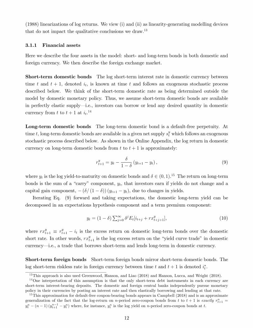
Long-term domestic bonds The long-term domestic bond is a default-free perpetuity. At

time t, long-term domestic bonds are available in a given net supply syt which follows an exogenous

stochastic process described below. As shown in the Online Appendix, the log return in domestic

currency on long-term domestic bonds from t to t+ 1 is approximately:

ryt+1 = yt −δ

1− δ (yt+1 − yt) , (9)

where yt is the log yield-to-maturity on domestic bonds and δ ∈ (0, 1).15 The return on long-term

bonds is the sum of a “carry”component, yt, that investors earn if yields do not change and a

capital gain component, − (δ/ (1− δ)) (yt+1 − yt), due to changes in yields.Iterating Eq. (9) forward and taking expectations, the domestic long-term yield can be

decomposed in an expectations hypothesis component and a term premium component:

yt = (1− δ)∑∞

j=0 δjEt[it+j + rxyt+j+1], (10)

where rxyt+1 ≡ ryt+1 − it is the excess return on domestic long-term bonds over the domestic

short rate. In other words, rxyt+1 is the log excess return on the “yield curve trade”in domestic

currency– i.e., a trade that borrows short-term and lends long-term in domestic currency.

Short-term foreign bonds Short-term foreign bonds mirror short-term domestic bonds. The

log short-term riskless rate in foreign currency between time t and t+ 1 is denoted i∗t .

13This approach is also used Greenwood, Hanson, and Liao (2018) and Hanson, Lucca, and Wright (2018).14One interpretation of this assumption is that the only short-term debt instruments in each currency are

short-term interest-bearing deposits. The domestic and foreign central banks independently pursue monetarypolicy in their currencies by posting an interest rate and then elastically borrowing and lending at that rate.15This approximation for default-free coupon-bearing bonds appears in Campbell (2018) and is an approximate

generalization of the fact that the log-return on n-period zero-coupon bonds from t to t + 1 is exactly rnt+1 =ynt − (n− 1) (yn−1t+1 − ynt ) where, for instance, ynt is the log yield on n-period zero-coupon bonds at t.

12

Long-term foreign bonds Long-term foreign bonds mirror long-term domestic bonds. They

are available in an exogenous, time-varying net supply sy∗t . The log return in foreign currency

on long-term foreign bonds is given by the analog of Eq. (9), and the log yield-to-maturity on

foreign bonds, y∗t , is given by the analog of Eq. (10). We use rxy∗

t+1 ≡ ry∗

t+1 − i∗t to denote theexcess return on the “yield curve trade”in foreign currency.

Foreign exchange Let Qt be the foreign exchange rate defined as units of domestic currency

per unit of foreign currency. An exchange rate of Qt means that an investor can exchange foreign

short-term bonds with a market value of one unit of foreign currency for domestic short-term

bonds with a market value of Qt in domestic currency. Thus, a rise in Qt means an appreciation

of the foreign currency relative to domestic currency. Let qt denote the log exchange rate.

Consider the excess return on foreign currency from time t to t + 1– i.e., the FX trade that

borrows short-term in domestic currency and lends short-term in foreign currency. The log excess

return on foreign currency is approximately:

rxqt+1 = (qt+1 − qt) + (i∗t − it). (11)

Thus, the excess return on foreign currency is the sum of a “carry” component, i∗t − it, that

investors earn if exchange rates do not change and a capital gain component, (qt+1 − qt), due tochanges in exchange rates. Assuming the exchange rate is stationary with a steady-state level of

qt = 0– i.e., that purchasing-power parity holds in the long run, we can iterate forward and take

expectations to obtain:

qt =∑∞

j=0Et[(i∗t+j − it+j)− rx

qt+j+1], (12)

as in Froot and Ramadorai (2005). Thus, the exchange rate is the sum of a UIP component and

an FX risk premium component.16

Real versus nominal rates Since our theory hinges on comovement between exchange rates

and short-term interest rates, it makes sense to think of the four interest rates in our model as real

interest rates and the exchange rate as the real exchange rate.17 This is why we focused on data

in recent decades– when inflation expectations have been firmly anchored and where movements

in nominal interest rates largely correspond to movements in real rates– in the previous section.

16Although UIP fails in our model, covered-interest-rate parity (CIP) will hold because the only friction in ourmodel is the limited risk-bearing capacity of bond investors and the CIP arbitrage trade is completely riskless forbond investors. However, it would be straightforward to capture the kinds of post-2008 CIP violations documentedby Du, Tepper, and Verdelhan (2018), Jiang, Krishnamurthy, and Lustig (2019), and Du, Hebert, and Huber(2019) by adding investor balance sheet constraints to the model as in, e.g., Garleanu and Pedersen (2011). And,in the presence of time-varying constraints, CIP violations would comove with bond and FX risk premiums.17If short-term nominal interest rates move one-for-one with expected inflation, then news about future inflation

will not impact real exchange rates. What is more, inflation news will not lead to unexpected changes in nominalexchange rates: it will only lead to expected future movements in nominal exchange rates. By contrast, newsabout future short-term real rates should always impact both real and nominal exchange rates.

13

3.1.2 Risk factors

Investors face two types of risk in our model: interest rate risk and supply risk. First, long-term

bonds are exposed to interest rate risk. For example, long-term domestic bonds will suffer an

unexpected loss if short-term domestic rates rise unexpectedly. Similarly, foreign exchange posi-

tions are exposed to interest rate risk: foreign currency will depreciate (appreciate) unexpectedly

if short-term domestic (foreign) rates rise unexpectedly. Second, both long-term bonds and FX

positions are exposed to supply risk: there are random supply shocks which impact equilibrium

bond yields and exchange rates, holding fixed the expected future path of short rates.

Short-term interest rates We assume short-term interest rates in domestic and foreign cur-

rencies follow symmetric AR(1) processes with correlated shocks. Specifically, we assume:

it+1 = ı+ φi(it − ı) + εit+1 , (13a)

i∗t+1 = ı+ φi(i∗t − ı) + εi∗t+1, (13b)

where ı > 0, φi ∈ (0, 1), V art[εit+1 ] = V art[εi∗t+1 ] = σ2i > 0, and ρ = Corr[εit+1 , εi∗t+1 ] ∈ [0, 1].

Net bond supplies We assume the net supplies of long-term domestic bonds (syt ) and long-

term foreign bonds (sy∗t ) follow symmetric AR(1) processes. Specifically, we assume:

syt+1 = sy + φsy(syt − sy) + εsyt+1, (14a)

sy∗t+1 = sy + φsy(sy∗t − sy) + εsy∗t+1 , (14b)

where sy > 0, φsy ∈ (0, 1), and V art[εsyt+1 ] = V art[εsy∗t+1 ] = σ2sy ≥ 0. These net bond supplies

should be viewed as the gross supply of long-term bonds minus the demand of any inelastic

“preferred habitat” investors– i.e., they reflect the combined supply and demand shocks that

global rates investors must absorb in equilibrium. Assuming that the two short rates and bond

supplies follow symmetric AR(1) processes enhances the analytical tractability of the model, but

it is easy to solve the model numerically if we relax these symmetry assumptions.18

Net FX supply We assume that global bond investors must engage in a borrow-at—home and

lend-abroad FX trade in time-varying quantity sqt to accommodate the opposing demand of other

unmodeled agents. Concretely, we assume:

sqt+1 = φsqsqt + εsqt+1 , (15)

where V art[εsqt+1 ] = σ2sq ≥ 0 and φsq ∈ (0, 1). Of course, if we consider all agents in the global

economy, then foreign exchange must be in zero net supply: if some agent is exchanging dollars

for euros, then some other agent must be exchanging euros for dollars. However, the specialized

18The Appendix discusses the impact of relaxing these symmetry assumptions on short rates and bond supply.

14

bond investors in our model are only a subset of all actors in global financial markets, so they

need not have zero foreign exchange exposure.

Collecting terms, let εt+1 ≡ [εit+1 , εi∗t+1 , εsyt+1 , εsy∗t+1, εsqt+1 ]

′ and Σ ≡ V art [εt+1]. For simplicity,

we assume the three supply shocks are independent of each other and of both short rates. Again,

this independence assumption enhances analytical tractability, but it is straightforward to solve

the model numerically for any arbitrary variance-covariance matrix Σ.

3.1.3 Global bond investors

The global bond investors in our model are specialized investors who choose portfolios consisting

of short-term and long-term bonds in the two currencies. They have a constant risk tolerance of

τ and have mean-variance preferences over wealth tomorrow. Let dyt (dy∗t ) denote bond investors’

holdings of long-term domestic (foreign) bonds and let dqt denote investors’position in the borrow-

at-home and lend-abroad FX trade.19 Thus, defining dt ≡ [dyt , dy∗t , d

qt ]′ and rxt+1 ≡ [rxyt+1, rx

y∗t+1,

rxqt+1]′, investors choose their portfolio holdings to solve

maxdt

{d′tEt [rxt+1]−

1

2τd′tV art [rxt+1] dt

}, (16)

so their demands must satisfy:

Et [rxt+1] = τ−1V art [rxt+1] dt. (17)

These preferences are similar to assuming that investors manage their overall risk exposure using

Value-at-Risk or other standard risk management techniques.

In practice, we associate the global bond investors in our model with market players such

as fixed-income divisions at global broker-dealers and large global macro hedge funds. Relative

to more broadly diversified players in global capital markets, risk factors related to movements

in interest rates loom large for these imperfectly diversified bond market players. Indeed, the

particular form of segmentation that we assume is quite natural since both government bonds

and foreign exchange are highly interest-rate sensitive assets. Specifically, any human capital or

physical infrastructure that is useful for managing interest-rate sensitive assets can be readily

applied to both bonds and foreign exchange.20

19Irrespective of whether global bond investors are domestic- or foreign-based, they solve (16). The idea isthat we can represent an investor’s positions in any asset other than short-term bonds in her local currency as alinear combination of these three long-short trades. So, assuming that all investors have the same risk toleranceand hold the same beliefs about returns, all global bond investors will choose the same exposures to these threelong-short trades regardless of whether they are based at home or abroad.20It is easy to allow for shocks to the aggregate risk tolerance of global bond investors. Specifically, if aggregate

risk tolerance at time t is τ t, demands satisfy Et [rxt+1] = τ−1t V art [rxt+1]dt. If the physical net supply of assetsthat investors must hold is st, the market-clearing conditions are dt = st, implying Et [rxt+1] = V art [rxt+1] τ

−1t st.

This is equivalent to our model with τ = 1 and st = τ−1t st. We would then assume the effective supplies st = τ−1t stfollow a VAR(1) process.

15

3.2 Equilibrium

3.2.1 Conjecture and solution

We need to pin down three equilibrium prices: yt, y∗t , and qt. To solve the model, we conjecture

that prices are linear functions of a 5 × 1 state vector xt = [it, i∗t , s

yt , s

y∗t , s

qt ]′. As shown in the

Online Appendix, a rational expectations equilibrium of our model is a fixed point of an operator

involving the “price-impact”coeffi cients which govern how the supplies st impact yt, y∗t , and qt.

Specifically, the market clearing condition dt = st implicitly defines an operator which gives

the expected returns– and, hence, the price-impact coeffi cients– that will clear markets when

investors believe the risk of holding assets is determined by some initial set of price-impact

coeffi cients. A rational expectations equilibrium of our model is a fixed point of this operator.

In the absence of supply risk (σ2sy = σ2sq = 0), this fixed-point problem is degenerate and

there is a straightforward, unique equilibrium. However, when asset supply is stochastic, the

fixed-point problem is non-degenerate: the risk of holding assets depends on how prices react

to supply shocks. For example, if investors believe supply shocks will have a large impact on

prices, they perceive assets as being highly risky. As a result, investors will only absorb supply

shocks if they are compensated by large price declines and high future expected returns, making

the initial belief self-fulfilling. This kind of logic means that (i) an equilibrium only exists when

investors’risk tolerance τ is suffi ciently large relative to the volatility of supply shocks and (ii)

the model admits multiple equilibria.21 However, there is at most one equilibrium that is stable

in the sense that it is robust to a small perturbation in investors’beliefs regarding equilibrium

price impact.22 We focus on the unique stable equilibrium in our analysis.

3.2.2 Equilibrium expected returns and prices

We now characterize equilibrium expected returns and prices. Market clearing implies that

dt = st. Thus, using equation (17), equilibrium expected returns must satisfy:

Et [rxt+1] = τ−1V art [rxt+1] st = τ−1Vst, (18)

21Equilibrium non-existence and multiplicity of this sort are common in models like ours where short-livedinvestors absorb shocks to the supply of infinitely-lived assets. Different equilibria correspond to different self-fulfilling beliefs that investors hold about the price-impact of supply shocks and, hence, the risks associated withholding assets. For previous treatments of these issues, see De Long, Shleifer, Summers, and Waldmann (1990),Spiegel (1998), Watanabe (2008), Banerjee (2011), Albagli (2015), and Greenwood, Hanson, and Liao (2018).22Consistent with Samuelson’s (1947) “correspondence principle,”this stable equilibrium has comparative stat-

ics that accord with standard intuition. By contrast, the comparative statics of the unstable equilibria are usuallycounterintuitive. For instance, at an unstable equilibrium, an increase in the volatility of short rate shocks canreduce the impact that supply shocks have on equilibrium prices. By contrast, in the unique stable equilibrium, anincrease in the volatility of short rate shocks always increases the impact of supply shocks on equilibrium prices.Furthermore, as supply risk grows small, the stable equilibrium converges to the equilibrium with no supply risk,whereas the unstable equilibria explode with extremely small supply shocks having a massive price impact.

16

where V = V art [rxt+1] is constant in equilibrium. Writing out Eq. (18) and making use of the

symmetry between long-term domestic and foreign bonds in equations (13) and (14), we have:

Et[rxyt+1

]=

1

τ[Vy × syt + Cy,y∗ × sy∗t + Cy,q × sqt ] (19a)

Et[rxy∗t+1

]=

1

τ[Cy∗,y × syt + Vy × sy∗t − Cy,q × sqt ] (19b)

Et[rxqt+1

]=

1

τ[Cy,q × (syt − sy∗t ) + Vq × sqt ] , (19c)

where Vy ≡ V art[rxyt+1] = V art[rx

y∗t+1], Cy∗,y ≡ Covt[rx

yt+1, rx

y∗t+1], andCy,q ≡ Covt[rx

yt+1, rx

qt+1] =

−Covt[rxy∗t+1, rxqt+1]. These variances and covariances are equilibrium objects: they depend both

on shocks to short-term interest rates and on the equilibrium price impact of supply shocks.

Making use of Eqs. (10) and (12) and the AR(1) dynamics for it, i∗t , syt , s

y∗t , and s

qt , we can

then characterize equilibrium yields and the exchange rate. The long-term domestic yield is:

yt =

Expectations hypothesis︷ ︸︸ ︷{ı+

1− δ1− δφi

× (it − ı)}

+

Steady-state term premium︷ ︸︸ ︷{τ−1 (Vy + Cy,y∗)× sy

}(20a)

+

{τ−1

1− δ1− δφsy

[Vy × (syt − sy) + Cy,y∗ × (sy∗t − sy)] + τ−11− δ

1− δφsqCy,q × sqt

}︸ ︷︷ ︸

Time-varying term premium

;

the long-term foreign yield is:

y∗t =

Expectations hypothesis︷ ︸︸ ︷{ı+

1− δ1− δφi

× (i∗t − ı)}

+

Steady-state term premium︷ ︸︸ ︷{τ−1 (Vy + Cy,y∗)× sy

}(20b)

+

{τ−1

1− δ1− δφsy

[Cy,y∗ × (syt − sy) + Vy × (sy∗t − sy)]− τ−11− δ

1− δφsqCy,q × sqt

}︸ ︷︷ ︸

Time-varying term premium

;

and the foreign exchange rate is

qt =

Uncovered interest rate parity︷ ︸︸ ︷{1

1− φi× (i∗t − it)

}−

FX risk premium︷ ︸︸ ︷{τ−1

1

1− φsyCy,q × (syt − sy∗t ) + τ−1

1

1− φsqVq × sqt

}. (20c)

Eqs. (20a) and (20b) say that long-term domestic and foreign yields are the sum of an ex-

pectations hypothesis piece that reflects expected future short-term rates and a term premium

piece that reflects expected future bond risk premia. For instance, the expectations hypothesis

component of long-term domestic rates depends on the current deviation of short-term domestic

rates from their steady-state level (i∗t − ı) and the persistence of short-term rates (φi). Similarly,the domestic term premium depends on the current deviation of asset supplies from their steady

state levels and the persistence of those asset supplies. Eq. (20c) says that the foreign exchange

17

rate consists of an uncovered interest rate parity (UIP) term, reflecting expected future foreign-

minus-domestic short rate differentials, minus a risk-premium term that reflects expected future

excess returns on the borrow-at-home lend-abroad FX trade.

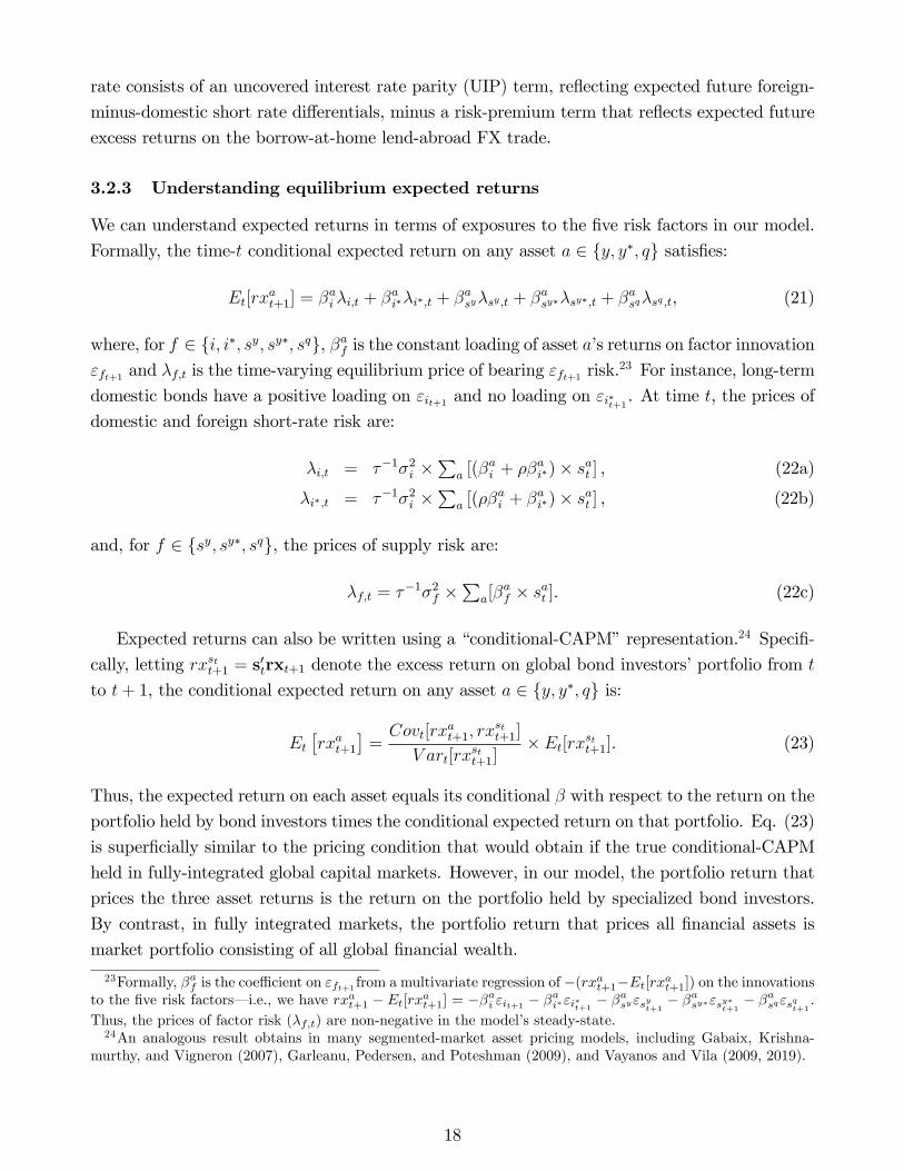
3.2.3 Understanding equilibrium expected returns

We can understand expected returns in terms of exposures to the five risk factors in our model.

Formally, the time-t conditional expected return on any asset a ∈ {y, y∗, q} satisfies:

Et[rxat+1] = βai λi,t + βai∗λi∗,t + βasyλsy ,t + βasy∗λsy∗,t + βasqλsq ,t, (21)

where, for f ∈ {i, i∗, sy, sy∗, sq}, βaf is the constant loading of asset a’s returns on factor innovationεft+1 and λf,t is the time-varying equilibrium price of bearing εft+1 risk.

23 For instance, long-term

domestic bonds have a positive loading on εit+1 and no loading on εi∗t+1. At time t, the prices of

domestic and foreign short-rate risk are:

λi,t = τ−1σ2i ×∑

a [(βai + ρβai∗)× sat ] , (22a)

λi∗,t = τ−1σ2i ×∑

a [(ρβai + βai∗)× sat ] , (22b)

and, for f ∈ {sy, sy∗, sq}, the prices of supply risk are:

λf,t = τ−1σ2f ×∑

a[βaf × sat ]. (22c)

Expected returns can also be written using a “conditional-CAPM”representation.24 Specifi-

cally, letting rxstt+1 = s′trxt+1 denote the excess return on global bond investors’portfolio from t

to t+ 1, the conditional expected return on any asset a ∈ {y, y∗, q} is:

Et[rxat+1

]=Covt[rx

at+1, rx

stt+1]

V art[rxstt+1]

× Et[rxstt+1]. (23)

Thus, the expected return on each asset equals its conditional β with respect to the return on the

portfolio held by bond investors times the conditional expected return on that portfolio. Eq. (23)

is superficially similar to the pricing condition that would obtain if the true conditional-CAPM

held in fully-integrated global capital markets. However, in our model, the portfolio return that

prices the three asset returns is the return on the portfolio held by specialized bond investors.

By contrast, in fully integrated markets, the portfolio return that prices all financial assets is

market portfolio consisting of all global financial wealth.

23Formally, βaf is the coeffi cient on εft+1 from a multivariate regression of −(rxat+1−Et[rxat+1]) on the innovationsto the five risk factors– i.e., we have rxat+1 − Et[rxat+1] = −βai εit+1 − βai∗εi∗t+1 − β

asyεsyt+1 − β

asy∗εsy∗t+1 − β

asqεsqt+1 .

Thus, the prices of factor risk (λf,t) are non-negative in the model’s steady-state.24An analogous result obtains in many segmented-market asset pricing models, including Gabaix, Krishna-

murthy, and Vigneron (2007), Garleanu, Pedersen, and Poteshman (2009), and Vayanos and Vila (2009, 2019).

18

3.3 Bond term premiums and exchange rates

The major payoff from our baseline model is that we are able to study the simultaneous de-

termination of domestic term premia, foreign term premia, and foreign exchange risk premia.

Specifically, we can ask how a shift in the supply on any of these three assets impacts the

equilibrium expected returns on the two other assets using Eq. (19).

3.3.1 Limiting case with no supply risk

Many of the core results of the model can be illustrated using the limiting case in which asset

supplies are constant over time, leaving only short rate risk– i.e., where σ2sy = σ2sq = 0.

Proposition 1 Equilibrium without supply shocks. If σ2sy = σ2sq = 0 and ρ ∈ (0, 1), then

Cy,q = (1− ρ)δ

1− δφi1

1− φiσ2i > 0. (24)

Cy,y∗ = ρ

(δ

1− δφi

)2σ2i > 0. (25)

Thus, ∂Et[rxqt+1]/∂s

yt = τ−1Cy,q is decreasing in the correlation between domestic and foreign

short rates, ρ, whereas ∂Et[rxy∗t+1]/∂s

yt = τ−1Cy,y∗ is increasing in ρ.

Proposition 1 provides guidance about how shifts in long-term bond supply– e.g., due to QE

policies– should impact exchange rates and term premiums. There are two key takeaways.25

First, Proposition 1 shows that a shift in domestic bond supply impacts the domestic term

premium, the foreign term premium, and the FX risk premium. For example, suppose there is

an increase in the supply of dollar long-term bonds. This increase in dollar bond supply raises

the price of bearing dollar short-rate risk in Eq. (22a), lifting the expected returns on the dollar

yield curve trade and thus dollar long-term yields as in Vayanos and Vila (2009, 2019). The

increase in dollar bond supply also raises the euro term premium and euro long-term yields when

ρ > 0.26 Turning to exchange rates, Eq. (20c) shows that the borrow-in-dollars to lend-in-euros

FX trade is also exposed to dollar short-rate risk: the euro depreciates when dollar short rates

rise through the standard UIP channel. Because the price of bearing dollar short-rate has risen,

the expected returns on the FX trade must also rise. Thus, an increase in the supply of long-term

dollar bonds leads the euro to depreciate; it is then expected to appreciate going forward.27

25Technically, the comparative statics in Proposition 1 must be interpretted as comparative statics on thesteady-state level of expected returns across economies where asset supplies are constant over time– i.e., theygive the effects of supply shifts that investors think are impossible. Nevertheless, the limiting case without supplyrisk highlights the core mechanism at the heart of our model.26This occurs even though long-term euro yields are not directly exposed to movements in dollar short rates.

Specifically, when ρ > 0, an increase in dollar bond supply raises the price of euro short-rate risk in Eq. (22b).Intuitively, since the euro yield-curve trade tends to suffer at the same time as the dollar yield-curve trade, anincrease in the supply of dollar bonds raises the expected return on the euro yield-curve trade.27More precisely, when ρ > 0, an increase in the supply of long-term dollar bonds raises the prices of both

dollar and euro short-rate risk per Eqs. (22a) and (22b). As shown in Eq. (20c), the FX trade has offsetting

19

Second, Proposition 1 shows that the effects of a shift in domestic bond supply depend on the

correlation ρ between domestic and foreign short-rates. When ρ is higher, more of the effect of the

domestic bond supply shift appears in long-term foreign yields and less shows up in the exchange

rate. For instance, U.S. short-term rates are more highly correlated with those in Europe than

those in Japan. Thus, Proposition 1 suggests we should expect U.S. QE– a reduction in dollar

bond supply– to lead to a larger depreciation of the dollar versus the Japanese yen than versus

the euro. At the same time, U.S. QE should lead to a larger reduction in European term premia

than Japanese term premia. Intuitively, if foreign and domestic short rates are highly correlated,

then the UIP component of the exchange rate will not be very volatile; if domestic short rates

rise, foreign short rates are also likely to rise, leaving the UIP component of the exchange rate

largely unchanged. This means that the FX trade is not very exposed to interest rate risk and,

therefore, its expected return should not move much in response to bond supply shifts.

3.3.2 Adding supply shocks

We now show that these results generalize once we add stochastic shocks to the net supplies of

domestic and foreign long-term bonds and to foreign exchange.28

Proposition 2 Equilibrium with supply shocks. If 0 ≤ ρ < 1, σ2sy ≥ 0, σ2sq ≥ 0, then in

any stable equilibrium we have ∂Et[rxqt+1]/∂s

yt = τ−1Cy,q > 0. If in addition ρ > 0 and σ2sq = 0,

then in any stable equilibrium we have ∂Et[rxy∗t+1]/∂s

yt = τ−1Cy,y∗ > 0. Thus, by continuity of

the stable equilibrium in the model’s underlying parameters, we have ∂Et[rxy∗t+1]/∂s

yt > 0 unless

foreign exchange supply shocks are especially volatile and ρ is near zero.

Proposition 2 shows that, once we allow supply to be stochastic, shifts in bond supply continue

to impact bond yields and foreign exchange rates as they did in Proposition 1 where supply was

fixed. Shifts in supply tend to amplify the comovement between long-term bonds and foreign

exchange that is attributable to shifts in short-term interest rates.

The exception is when FX supply shocks are especially volatile (σ2sq is large) and the corre-

lation of short rates ρ is low. Because FX supply shocks push domestic and foreign long-term

yields in opposite directions by Eq. (20), if these shocks are highly volatile they can result in a

negative equilibrium correlation between domestic and foreign bond returns, Cy,y∗, even if the

underlying short rates are positively correlated. However, in the empirically relevant case where

ρ is meaningfully positive, we have Cy,y∗ > 0 and bond yields behave as in Proposition 1.

exposures to dollar and euro short rates due to standard UIP logic. However, when the two short rate processesare symmetric as in Eq. (13), the exposure to dollar short rates dominates and we have ∂Et[rx

qt+1]/∂s

yt > 0.

28As shown in the Online Appendix, when σ2sy > 0 and σ2sq > 0, solving the model involves characterizing the

stable solution to a system of four quadratic equations in four unknowns. When σ2sy > 0 and σ2sq = 0, the model

can be solved analytically: we simply need to solve two quadratics and a linear equation.

20

3.3.3 Empirical implications of the baseline model

In Section 2, we presented evidence for three propositions. First, exchange rates appear to

be about as sensitive to changes in long-term interest rate differentials as they are to changes

in short-term interest rate differentials. Second, the component of long rate differentials that

matters for exchange rates appears to be a term premium differential. Third, the term premium

differentials that move exchange rates appear to be, at least in part, quantity-driven. Using our

baseline model, we can now formally motivate these empirical results.

For simplicity, we focus on the case where FX supply shocks are small– i.e., the limit where

sqt = 0 and σ2sq = 0.29 In this case, the foreign exchange risk premium is decreasing in the

difference between foreign and domestic bond supply (sy∗t − syt ),

Et[rxqt+1

]=

<0︷ ︸︸ ︷[−τ−1Cy,q

]× (sy∗t − syt ) , (26)

and the difference between foreign and domestic bond risk premiums is increasing in sy∗t − syt :

Et[rxy∗t+1 − rx

yt+1

]=

>0︷ ︸︸ ︷[τ−1 (Vy − Cy,y∗)

]× (sy∗t − syt ) . (27)

Eqs. (26) and (27) motivate our regressions examining QE announcement dates in Section 2. In

the context of the model, we think of a euro QE announcement as news indicating that the supply

of euro long-term bonds sy∗t will be low. Eq. (27) shows that this decline in euro bond supply

should reduce euro term premia relative to dollar term premia. And, Eq. (26) shows that this

decline in sy∗t should increase the risk premium on the borrow-in-dollar lend-in-euros FX trade,

leading the euro to depreciate relative to the dollar. By symmetry, U.S. QE announcements– i.e.,

news that syt will be low– will have the opposite effects.

Combining Eqs. (26) and (27), the FX risk premium is negatively related to the difference

between foreign and domestic bond risk premia:

Et[rxqt+1

]=

<−1︷ ︸︸ ︷[− Cy,qVy − Cy,y∗

]× Et

[rxy∗t+1 − rx

yt+1

]. (28)

Eq. (28) motivates the tests in Section 2 where we forecast foreign exchange returns using the

difference in (proxies for) foreign and domestic term premia. When euro bond supply is high,

the euro term premium is high and the risk premium on the borrow-in-dollar lend-in-euro FX

trade is low. Thus, the FX risk premium moves inversely with the foreign term premium. The

same argument applies to the domestic term premium with the opposite sign– i.e., the FX risk

premium moves proportionately with the domestic term premium.30

29The Online Appendix shows that a similar, albeit slightly more complicated, set of results obtains whenσ2sq > 0 and s

qt 6= 0.

30The constant of proportionality in Eq. (28), −Cy,q/ (Vy − Cy,y∗), is less than −1 because foreign exchange is

21

Combining Eq. (12) and (28), the exchange rate reflects the sum of expected (i) foreign-minus-

domestic short rate differentials and (ii) foreign-minus-domestic bond risk-premium differentials:

qt =∑∞

j=0Et[i∗t+j − it+j] +

>1︷ ︸︸ ︷[Cy,q

Vy − Cy,y∗

]×∑∞

j=0Et[rxy∗t+j+1 − rx

yt+j+1]. (29)

This result motivates the tests in Table 1 and 2 where we regress changes in exchange rates

on changes in short rate differentials and changes in (proxies for) term premium differentials.

When foreign bond supply is high, the foreign term premium is high and the risk premium on

the borrow-at-home to lend-abroad FX trade is low. For investors to earn low returns on foreign

currency, foreign currency must be strong– qt must be high– and must be expected to depreciate.

Lastly, our model can match the otherwise puzzling finding in Lustig, Stathopoulos, and

Verdelhan (2019) that the return to the FX trade– conventionally implemented by borrowing

and lending short-term in different currencies– declines if one borrows long-term in the currency

with low rates and lends long-term in the currency with high rates. To see this, note that the

return on a long-term FX trade that borrows long-term at home to lend long-term abroad is

just a combination of our three long-short returns. Specifically, the return on this long-term FX

trade equals (i) the return to borrowing long to lend short at home (−rxyt+1), plus (ii) the returnto borrowing short at home to lend short abroad (rxqt+1), plus (iii) the return to borrowing short

abroad to lend long abroad (rxy∗t+1). Thus, the expected return on the long-term FX trade is:

Et[rxqt+1 +

(rxy∗t+1 − rx

yt+1

)]=

∈(0,1)︷ ︸︸ ︷[1− Vy − Cy,y∗

Cy,q

]× Et

[rxqt+1

]. (30)

Eq. (30) shows that the expected return on the long-term FX trade is smaller in absolute

magnitude– and hence less volatile over time– than that on the standard short-term FX trade.

The intuition is that the long-term FX trade has offsetting exposures that reduce its riskiness

for global rates investors as compared to the standard FX trade. For instance, the standard FX

trade (rxqt+1) will suffer when there is an unexpected increase in domestic short rates. However,

borrowing-long to lend-short in domestic currency (i.e., −rxyt+1) will profit when there is anunexpected rise in domestic rates. Thus, the long-term FX trade is less exposed to interest rate

risk than the standard short-term FX trade. As a result, the expected return on the long-term

FX trade moves less than one-for-one with that on the standard short-term FX trade.

We collect these observations in the following proposition:

Proposition 3 Empirical implications. Suppose ρ ∈ (0, 1), σ2sy > 0, and σ2sq = 0. Then:

• The FX risk premium (Et[rxqt+1

]) is decreasing in the difference in net long-term bond

supply between foreign and domestic currency (sy∗t − syt ). The difference between foreign

and domestic bond risk premia, Et[rxy∗t+1 − rx

yt+1

], is increasing in sy∗t − syt .

effectively a “longer duration”asset than long-term bonds.

22

• Et[rxqt+1

]is negatively related to Et

[rxy∗t+1 − rx

yt+1

].

• The foreign exchange rate (qt) is the sum of expected future foreign-minus-domestic short-

rate differentials and a term that is proportional to expected future foreign-minus-domestic

bond risk premium differentials.

• The expected return on the borrow-long-in-domestic to lend-long-in-foreign FX trade(Et

[rxqt+1 +

(rxy∗t+1 − rx

yt+1

)]) is smaller in magnitude than that on the standard borrow-

short-in-domestic to lend-short-in-foreign FX trade, (Et[rxqt+1

]).

3.4 A unified approach to carry trade returns

In this subsection, we show that our model can deliver a unified explanation that links foreign

exchange return predictability and bond return predictability. For foreign exchange, Fama (1984)

showed that the expected return on the borrow-at-home to lend-abroad FX trade is increasing

in the foreign-minus-domestic short rate differential, i∗t − it. This is the best known and mostempirically robust failure of uncovered interest rate parity. For long-term bonds, Fama and Bliss

(1987) and Campbell and Shiller (1991) showed that the expected return on the borrow-short

to lend-long yield curve trade is increasing in the slope of the yield curve or the “term spread,”

yt − it. This is arguably the best known and most empirically robust failure of the expectationshypothesis of the term structure. In other words, the expected excess returns on both the FX

trade and the yield curve trade are increasing in their “carry,”defined as the return that investors

will earn if asset prices remain unchanged.

The baseline model we developed above does not generate either the Fama (1984) result for

the FX trade or the Campbell and Shiller (1991) result for the yield curve trade. In our baseline

model, shocks to short-term interest rates make foreign exchange and long-term bonds risky

investments for global rates investors. However, the level of short-term interest rates does not

affect expected excess returns on foreign exchange and long-term bonds.

However, a simple extension of our model can simultaneously match these two facts if we follow

Gabaix and Maggiori (2015) and, appealing to balance-of-trade flows, assume that global rates

investors’exposure to foreign currency is increasing in the strength of the foreign currency. Put

simply, our model makes it possible to “kill two birds with one stone.”Specifically, the assumption

that Gabaix and Maggiori (2015) needed to make to match the Fama (1984) pattern within a

segmented-markets model of the foreign exchange market, immediately delivers the Campbell-

Shiller (1991) result for both the domestic and foreign yield-curve trades. Symmetrically, the

assumption that Vayanos and Vila (2009, 2019) needed to make to match the Campbell-Shiller

(1991) fact within a segmented-markets model of the term structure– i.e., that the net supply

of long-term bonds is decreasing in the level of long-term yields– immediately delivers the Fama

(1984) pattern for foreign exchange in our model.

Concretely, we extend the model by allowing the net supplies to depend on equilibrium prices:

23

nyt = syt − Syyt, (31a)

ny∗t = sy∗t − Syy∗t , (31b)

nqt = sqt + Sqqt, (31c)

where Sq, Sy ≥ 0. For example, the assumption that Sq > 0 follows Gabaix and Maggiori (2015)

and is a reduced-form way of modeling balance-of-trade flows in the FX market. Specifically,

assume the domestic country runs a trade surplus of Sqqt with the foreign country: when foreign

currency is strong, domestic exports rise and domestic imports decline. However, if the domestic

country is running a trade surplus, domestic exporters will want to swap the foreign currency

they receive from their foreign sales for domestic currency. By FX market clearing, global bond

investors must take the other side of these trade-driven flows. Thus, when foreign currency is

strong, the expected returns on foreign exchange must rise to induce global bond investors to

increase their exposure to foreign currency. As Gabaix and Maggiori (2015) show, assuming that

Sq > 0 in this way delivers the Fama (1984) result for foreign exchange markets.

We solve the extended model using the same approach that we used to solve the baseline

model.31 The comparative statics of expected returns with respect to the independent supply

shocks– syt , sy∗t , and s

qt– in this extension are similar to those in the baseline model. However,

in this extension, it and i∗t impact now expected returns on the three carry trades.

Proposition 4 Matching Fama (1984) and Campbell-Shiller (1991). Suppose ρ < 1. If

(i.a) Sq > 0 and Sy = 0 or (i.b) Sq = 0 and Sy > 0 and (ii) there are no independent supply

shocks (σ2sy = σ2sq = 0), then ∂Et[rxqt+1

]/∂i∗t = −∂Et

[rxqt+1

]/∂it > 0. Since exchange rates are

less responsive to short rates than under UIP, if one estimates the time-series regression:

rxqt+1 = αq + βq × (i∗t − it) + ξqt+1, (32)

one obtains βq = ∂Et[rxqt+1]/∂i

∗t > 0 as in Fama (1984).

Under the same conditions, we also have ∂Et[rxyt+1

]/∂it = ∂Et

[rxy∗t+1

]/∂i∗t < 0. Thus, long-

term yields are less responsive to movements in short rates than under the expectations hypothesis,

so expected returns on long-term bonds are high when short rates are low. Furthermore, since

the term spread is high when short rates are low, if one estimates the time-series regressions:

rxyt+1 = αy + βy × (yt − it) + ξyt+1 and rxy∗t+1 = αy∗ + βy∗ × (y∗t − i∗t ) + ξy∗t+1, (33)

one obtains βy = βy∗ > 0 as in Campbell and Shiller (1991).

To see the logic, assume σ2sy = σ2sq = 0– i.e., there are no independent supply shocks, so net

31Specifically, the demands dt of global rates investors are still given by Eq. (17) above. Stacking the netsupplies in Eq. (31) as nt =

[nyt , n

y∗t , n

qt

]′, the market clearing conditions become dt = nt. Thus, equilibrium

returns satisfy Et [rxt+1] = τ−1V art [rxt+1]nt.

24

supplies only fluctuate because of movements in short-rates. In this case, we have

Et[rxqt+1

]= τ−1 [Cy,qSy × (y∗t − yt) + Vq × Sqqt] , (34)

and

Et[rxyt+1 − rx

y∗t+1

]= τ−1 [(Vy − Cy∗,y)Sy × (y∗t − yt) + 2Cy,qSq × qt] . (35)

First, assume Sq > 0 and Sy = 0 and suppose that i∗t − it > 0– i.e., that euro short rates

exceed dollar short rates. By standard UIP logic, the positive short-rate differential means that

the euro will be strong– i.e., qt will be high. The assumption that Sq > 0 implies that U.S. net

exports will be high, so U.S. exporters will want to convert their euro sales back to dollars. The

need to absorb these trade-driven FX flows means that global bond investors must bear greater

exposure to the euro when the euro is strong, raising the expected returns on the borrow-in-

dollar lend-in-euro FX trade. As a result, the expected return on the FX trade is increasing in

the euro-minus-dollar short-rate differential as in Fama (1984). This mechanism allows Gabaix

and Maggiori (2015) to match the Fama (1984) result. However, because these FX exposures

mean that global bond investors will lose (make) money if dollar (euro) short rates rise, the

equilibrium expected returns on the dollar (euro) yield curve trade must also rise (fall). Since

the U.S. term structure will steeper when i∗t − it > 0 by standard expectations-hypothesis logic,

the extended model will match Campbell and Shiller’s (1991) finding that a steep term structure

predicts high excess returns on long-term bonds.32

Another way to simultaneously match these two facts within our model is to follow Vayanos

and Vila (2009, 2019) who assume the net supply of long-term bonds is decreasing in the level

of long-term yields– i.e., to assume that Sy > 0. This would be the case if, as in the data, firms

and governments tend to borrow long-term when the level of interest rates is low, or if there are

“yield-oriented investors”who tend substitute away from long-term bonds and towards equities

when interest rates are low. As Vayanos and Vila (2009, 2019) show, assuming that Sy > 0

delivers the Campbell-Shiller (1991) result for long-term bonds. Specifically, assume Sy > 0 and

Sq = 0 and suppose that i∗t − it > 0. By standard expectations hypothesis logic, euro long-term

rates will be higher than dollar long-term rates, but the yield curve will be steeper in dollars since

dollar short rates will be expected to rise more over time. However, since the net supply of long-

term bonds is decreasing in long-term yields, the term premium component of long-term yields

will be larger in dollars than in euros, matching Campbell-Shiller (1991). However, the resulting

difference between dollar and euro long-term bond supply means that global bond investors will

have a larger exposure to dollar short-rate shocks, so the expected return on the FX trade will

also be positive. As a result, the expected return on the FX trade will be increasing in the

difference between euro and dollar short-term rates, matching the Fama (1984) pattern.

32Term spreads also positively forecast bond returns in our baseline model since supply shocks move yields andexpected returns on long-term bonds in the same direction. What is novel here is that term spreads forecast bondreturns even in the absence of independent supply shocks.

25

3.5 Relationship to consumption-based models

Our quantity-driven, segmented-markets model provides a unified way of jointly understanding

term premiums and foreign exchange rates. Thus, it is natural to contrast our model’s implica-

tions with those of frictionless consumption-based asset pricing models. Table 6 compares our

model’s implications with those of leading consumption-based models. We focus on real interest

rates and exchange rates since, as noted above, our theory speaks most naturally real returns.

Empirically, short-term real interest rates typically rise in economic expansions (and fall in

recessions)– e.g., because central banks adjust nominal short rates cyclically and since nominal

prices are sticky. In our model, specialized bond investors must take long positions in long-

term bonds (i.e., syt , sy∗t > 0). While rapid economic expansions are good times for the typical

household in the economy, they are actually bad times for the specialized bond investors because

specialists will suffer large capital losses on their long-term bond holdings. Thus, as in Vayanos

and Vila (2009, 2019), long-term bonds are risky for specialized investors and real term premiums

will be positive in our model. In most consumption-based models, short-term real rates also rise

in good economic times (and fall in bad times). However, this means that long-term real bonds

are a macroeconomic hedge for the representative household, implying that real term premiums

are negative and the real term structure should be downward sloping on average.33 Empirically,

however, real term structures are usually upward sloping, just like the nominal term structures.34

Consumption-based models also imply very different comovement patterns between foreign

exchange rates and real interest rates than those implied by our model. In consumption-based

models, foreign currency appreciates in bad times for foreign agents (and depreciates in bad times

for domestic agents). These exchange rate dynamics make domestic assets risky for foreign agents

(and foreign assets risky for domestic agents), rationalizing imperfect international risk sharing

even with complete financial markets.35 However, since foreign interest rates fall in bad foreign

times in most consumption-based models, the price of long-term foreign bonds rises in bad foreign

times. (Symmetrically, in bad domestic times, foreign currency depreciates and price of long-

term domestic bonds rises). Thus, realized foreign currency returns are positively (negatively)

correlated with those on long-term foreign (domestic) bonds. As a result, FX risk premium are

increasing in the foreign-minus-domestic term premium differential in most consumption-based

models (i.e., Covt[rxqt+1, rx

y∗t+1 − rx

yt+1

]> 0 and Et[rx

qt+1] is positively related to Et[rx

y∗t+1 −

rxyt+1]). By contrast, in our theory as in the data, the realized returns on foreign currency are

negatively (positively) correlated with those on long-term foreign (domestic) bonds. This is

33To be sure, there are consumption-based models where real interest rates rise in recessions, implying a positivereal term premium (e.g., Wachter [2006]). Empirically, however, real interest rates tend to fall in recessions.34The U.S. real curve has been upward sloping over 90% of the time from 1999 to present. The U.K. real curve

has been upward sloping nearly 75% of the time since 1986. And, for both countries, the relevant figures for thereal yield curve are similar to those for the nominal curve.35Since foreign short rates decline in bad foreign times in most consumption-based models, there is a standard

“UIP effect” that pushes foreign currency to depreciate in bad foreign times. However, by construction, thisUIP effect needs to more than fully offset in consumption-based models by either a temporary appreciation offoreign currency (i.e., by news that the expected returns on foreign currency will be lower going forward) or bya permanent appreciation (i.e., an innovation to a random walk component of the exchange rate).

26

because the realized returns on foreign exchange and long-term bonds are both driven by shocks

to short-term interest rates. As a result, the expected return on foreign currency is negatively

related to the foreign-minus-domestic term premium differential.

Finally, our model is capable of jointly matching the Fama (1984) “carry trade”pattern for

foreign exchange rates and the Campbell-Shiller (1991) “carry trade”pattern for long-term real

bonds. While consumption-based models are capable of matching the Fama (1984) pattern for

foreign exchange (see, e.g., Verdelhan [2010] and Bansal and Shaliastovich [2012]), they struggle

to simultaneously match the Campbell-Shiller (1991) pattern for real bonds in a realistic fashion.

Consider, for instance, Verdelhan (2010) who builds a habit formation model of foreign exchange

in the tradition of Campbell and Cochrane (1999). Suppose domestic agents are closer to their

habit level of consumption than foreign agents, so domestic agents are currently more risk averse.

Since the precautionary savings effect dominates the intertemporal substitution effect in Verdel-

han’s (2010) model, domestic short-term rates will be below foreign short rates. And, because

domestic agents are more risk averse, the expected excess returns to holding foreign currency

must be positive, thereby generating the Fama (1984) pattern. However, since interest rates

decline in bad economic times in Verdelhan (2010), long-term real bonds hedge macroeconomic

risk and carry a negative risk premium. Furthermore, bond risk premiums are more negative

when short rates are low. Thus, if the Verdelhan (2010) model is calibrated so the term structure

is steep when short rates are low– as is manifest in the data, the model delivers a negative asso-

ciation between the term spread and bond risk premiums, contrary to Campbell-Shiller (1991).36

The same is true for Bansal and Shaliastovich (2012), who build a long-run risks model of foreign

exchange in the tradition of Bansal and Yaron (2004).

In summary, Table 6 shows that our model is able to simultaneously match a large number of

important stylized facts about long-term bonds and foreign exchange rates. By contrast, leading

consumption-based models struggle to simultaneously match these stylized facts.

4 Further segmenting the global bond market

In Section 3, we showed that we can match several important empirical regularities about term

premiums and exchange rates using a simple segmented-markets model in which the marginal

investors in the global bond market are specialized bond investors. While this simple approach

is appealing, it does not capture two significant real-world features of bond and foreign exchange

markets. First, real-world markets feature a variety of different investor types– each facing a

different set of constraints– opening the door to meaningful segmentation within the global bond

market. Second, real world bond and foreign exchange markets involve substantial trading flows

between different investor types (Evans and Lyons [2002] and Froot and Ramadorai [2005]).

In this section, we further segment the global bond market as in Gromb and Vayanos (2002),

assuming some bond investors cannot trade short- and long-term bonds in both currencies. A

36It is also possible to calibrate the Verdelhan (2010) model to match the Campbell-Shiller (1991) pattern, butone then needs the yield curve to be flatter (less inverted) when short rates are low, which is counterfactual.

27

first key take-away from this extension is that, with further segmentation, exogenous bond supply

shocks give rise to endogenous trading flows in the foreign exchange market that are associated

with changes in exchange rates. A second key take-away is that a small amount of additional

segmentation always increases the impact of bond supply shocks on exchange rates. Furthermore,

unless market segmentation is extreme, bond supply shocks have a larger impact on exchange

rates than in our baseline model.

Our extended model features four types of bond investors. All types have mean-variance

preferences over one-period-ahead wealth and a risk tolerance of τ . Types only differ in their

ability to trade different assets. Specifically:

1. Domestic bond specialists, present in mass µπ, can only choose between short- and long-

term domestic bonds– i.e., they can only engage in the domestic yield curve trade. Thus,

their demand for long-term domestic bonds is byt = τ(V art

[rxyt+1

])−1Et[rxyt+1

].

2. Foreign bond specialists, also present in mass µπ, can only choose between short- and long-

term foreign bonds– i.e., they can only engage in the foreign yield curve trade. Their

demand for long-term foreign bonds is by∗t = τ(V art

[rxy∗t+1

])−1Et[rxy∗t+1

].

3. FX specialists, present in mass µ (1− 2π), can only choose between short-term domestic

and foreign bonds– i.e., they can only engage in the FX trade. Their demand for the

borrow-at-home-lend-abroad FX trade is bqt = τ(V art

[rxqt+1

])−1Et[rxqt+1

].

4. Global bond investors, present in mass (1− µ), can hold short- and long-term bonds in

both currencies and can engage in all three long-short trades. Their demand for the three

trades is dt = τ (V art [rxt+1])−1Et [rxt+1].

We assume µ ∈ [0, 1] and π ∈ (0, 1/2). Increasing the combined mass of specialist types, µ,

is equivalent to introducing greater segmentation in the global bond market. Thus, our baseline

model corresponds to the limiting case where µ = 0. At the other extreme, markets are fully

segmented when µ = 1. And, when µ ∈ (0, 1) markets are partially segmented.

Our domestic bond specialists are reminiscent of the specialized bond investors in Vayanos

and Vila (2009, 2019) in the sense that their positions in long-term domestic bonds are a suffi cient

statistic for the expected returns on the domestic yield curve trade. Our FX specialists are similar

to the FX intermediaries in Gabaix and Maggiori (2015): their FX positions are a suffi cient

statistic for the expected returns on the FX trade. In practice, we associate the domestic and

foreign bond specialists with market participants who, for institutional reasons, exhibit significant

home-bias and are essentially unwilling to substitute between bonds in different currencies. And,

we associate FX specialists with the global commercial banks who play an outsized role in the

foreign exchange market, but, who, are not natural holders of long-term bonds in either currency.

It is straightforward to solve for equilibrium under further segmentation. Letting [diag (V)]

be the matrix with the diagonal elements ofV = V art [rxt+1] on its diagonal and zeros elsewhere,

the vector of specialist investor demands is bt = [byt , by∗t , b

qt ]′= τ [diag (V)]−1Et [rxt+1]. Letting

28

Π = diag (π, π, 1− 2π), the market clearing conditions become st = µΠbt + (1− µ) dt, which

implies that equilibrium expected returns are given by:

Et [rxt+1] = τ−1[µΠ [diag (V)]−1 + (1− µ) V−1

]−1st. (36)

With this characterization, we can demonstrate the following results:

Proposition 5 Further segmenting the bond market. Suppose ρ < 1, σ2sy ≥ 0, σ2sq ≥ 0.

Suppose fraction µ of investors are specialists. We have the following results:

(i.) Segmentation leads to endogenous trading flows. For any µ ∈ (0, 1), a shock to the

supply of any asset a ∈ {y, y∗, q} triggers trading in all assets a′ 6= a between global bond

investors and specialist investors.

(ii.) (a) Greater segmentation increases own-market price impact. Formally, for anya ∈ {y, y∗, q}, ∂2Et[rxat+1]/∂sat ∂µ > 0. (b) Segmentation has a hump-shaped ef-fect on cross-market price impact. Formally, for any a ∈ {y, y∗, q} and a′ 6= a,∣∣∂Et[rxat+1]/∂sa′t ∣∣ is hump-shaped function of µ with ∣∣∂Et[rxat+1]/∂sa′t ∣∣ > 0 in our baseline

model (µ = 0) and ∂Et[rxat+1]/∂sa′t = 0 under full segmentation (µ = 1). (c) Overall,

greater segmentation increases bond market-wide price impact. For any supplyst 6= 0, the expected return on the global bond market portfolio rxstt+1 = s′trxt+1 is increasing

in µ: ∂Et[rxstt+1]/∂µ > 0.

(iii.) If asset supply is stochastic, greater segmentation increases market volatility.Formally, for any arbitrary bond portfolio pt 6= 0 with returns rxptt+1 = p′trxt+1, we have

∂V art[rxptt+1]/∂µ > 0. (If asset supply is constant, volatility is independent of µ.)

Increasing µ– i.e., further segmenting the global rates markets– has two direct effects on the

market equilibrium. First, as we increase µ, risk sharing becomes less effi cient because fewer

investors can absorb a given supply shock. For instance, the fraction of investors who can absorb

a shock to domestic bond supply is µπ + (1− µ), which is decreasing in µ. This gives rise to an

“ineffi cient risk-sharing”effect. Second, as we increase µ, we replace global bond investors whose

demands take the correlations between the three assets into account with specialist investors

who, taken as a group, behave as if the three returns are uncorrelated. This gives rise to a

“width of the pipe”effect: price impact is only transmitted across markets to the extent there

are investors– “the pipe”– whose demands are impacted by shocks to other markets. Finally,

there is a third indirect effect of increasing segmentation. To the extent that greater segmentation

directly raises the price impact of supply shocks, greater segmentation amplifies return volatility,

further increasing price impact. This is an “endogenous risk effect.”

As we raise µ, these three effects always increase the impact of a supply shock in market a, sat ,

on expected returns in that market: ∂2Et[rxat+1]/∂sat ∂µ > 0 for any a ∈ {y, y∗, q}. Cross-market

price impact under partial segmentation is more complicated. For instance, consider how the

29

FX risk premium responds to domestic bond supply, ∂Et[rxqt+1]/∂s

yt , as a function of µ. When

there are only global rates investors (µ = 0), a shock to domestic bond supply raises expected

returns on the FX trade: ∂Et[rxqt+1]/∂s

yt > 0. This is the key result from our baseline model.

By contrast, it is clear that ∂Et[rxqt+1]/∂s

yt = 0 when there are no global rates investors (µ = 1).

In this case, markets are completely segmented and bond supply shocks have no impact on the

foreign exchange market. In between, however, µ has a hump-shaped effect on cross-market

price impact. This hump-shape reflects the combination of the ineffi cient risk-sharing effect,

which typically leads ∂Et[rxqt+1]/∂s

yt to rise with µ and dominates when µ is near 0, and the

width of the pipe effect, which typically leads ∂Et[rxqt+1]/∂s

yt to fall with µ and dominates when

µ is near 1. Furthermore, the endogenous risk effect amplifies the net of these two effects, so the

hump-shaped pattern is more pronounced when there is more supply risk.

These results are illustrated in Figure 2.37 Panel A of Figure 2 plots the impact on expected

returns of a domestic bond supply shock as a function of µ. The plot assumes π = 1/3, so

specialists are evenly split between domestic bonds, foreign bonds, and foreign exchange. The

plot shows that, while ∂Et[rxyt+1]/∂s

yt is always increasing in µ, segmentation has a hump-shaped

effect on ∂Et[rxqt+1]/∂s

yt (and ∂Et[rx

y∗t+1]/∂s

yt ). Unless µ is near 1 and the global rates markets

is highly segmented, the effect of bond supply shocks on foreign exchange exceeds that in our

baseline model where µ = 0. Thus, it is natural to conjecture that the impact of bond supply

shocks on foreign exchange markets has risen in recent decades because µ has fallen over time.

In other words, relative to earlier periods where markets were extremely segmented (µ ≈ 1), the

global rates market has gradually become more integrated, raising ∂Et[rxqt+1]/∂s

yt (Mylonidis

and Kollias [2010], Pozzi and Wolswijk [2012]).

The next two plots in Panel B of Figure 2 show the trading response to a unit domestic bond

supply shock as a function of µ. When µ ∈ (0, 1), markets are partially segmented, meaning that

global bond investors and the three specialist types disagree on the appropriate compensation for

bearing factor risk exposure. Following a supply shock to any one asset, global bond investors

trade across markets to align– but not equalize– the way that factor risk is priced in different

markets. For instance, a shock to the supply of domestic bonds leads to foreign exchange trading

between global bond investors and FX specialists. Specifically, following a positive shock to

domestic bond supply, global bond investors want to increase their exposure to domestic bonds

and reduce their exposure to the FX trade. Foreign exchange specialists must take the other side,

increasing their exposure to the FX trade. These endogenous FX trading flows are associated

with an increase in FX risk premia and a depreciation of foreign currency.

37To draw Figures 2 and 3, we assume there is some FX-specific fundamental risk: we assumelimT→∞Et [qt+T ] = q∞t follows a random walk q∞t+1 = q∞t + εq∞,t+1 with V art [εq∞,t+1] = σ2q∞ > 0, imply-ing qt = q∞t +

∑∞j=0Et[(i

∗t+j − it+j)− rx

qt+j+1]. If σ

2q∞ = 0, then in the absence of supply risk, FX is a redundant

asset: FX returns are a linear combination of those on domestic and foreign bonds. Thus, if we instead assumedσ2q∞ = 0 in Figure 2, global bond investors would take very large long-short positions as µ approached 1 since theywould face no fundamental risk and would only be exposed to supply risk. Furthermore, while cross-market impactwould still be hump-shaped when σ2sq , σ

2sy > 0, instead of the smooth plots in Figure 2, there would be a sudden

decline in cross-market impact once µ became very close to 1. Indeed, in the limit where σ2q∞ = σ2sq = σ2sy = 0,cross-market impact would increase in µ for all µ ∈ (0, 1) and then discontinuosly vanish at µ = 1.

30

In this way, our extension with additional bond market segmentation endogenizes the kinds

of capital market driven FX flows considered in Gabaix and Maggiori (2015). Rather than being

exogenous quantities that specialist FX investors are required to absorb, these endogenous FX

flows are tied to supply-and-demand shocks for long-term domestic or foreign bonds.

5 The role of foreign exchange hedging

In this section, we show that adding investors who cannot hedge foreign exchange risk– i.e.,

investors who effectively “staple” the returns on foreign exchange together with other excess

returns– amplifies the effect of supply shocks on exchange rates. Going further, such return

stapling means that a broader set of financial shocks may impact exchange rates.

5.1 Unhedged bond investors

A variety of institutional frictions, including constraints on short-selling or using derivatives, may

constrain certain investors’ability to hedge foreign exchange risk. To capture such investors,

we add unhedged domestic and foreign bond investors to the model– i.e., investors who cannot

separately manage the FX exposure resulting from any investments they make in non-local, long-

term bonds. For example, if unhedged domestic investors want to buy long-term foreign bonds

to capture the foreign term premium, they must take on exposure to foreign currency. Thus,

unlike global rates investors, who can separately manage their exposures to foreign currency and

the foreign yield-curve trades, these unhedged domestic investors always “staple together” the

returns on the FX trade and the foreign yield curve trade.

Adding unhedged bond investors is like introducing a particular form of market segmentation.

As a result, supply shocks in one asset lead to trading in other related assets. Furthermore, we

show that adding unhedged bond investors always amplifies the impact of bond supply shocks

on the FX market relative to our baseline model.

We assume there are three investor types– all with mean-variance preferences over one-period-

ahead wealth and risk tolerance τ– who only differ in terms of the assets they can trade:

1. Unhedged domestic investors are present in mass η/2. They can trade short-term domestic

bonds, long-term domestic bonds, and long-term foreign bonds, but not short-term foreign

bonds. Thus, if they buy long-term foreign bonds, they must take on foreign exchange

exposure, generating an excess return of rxy∗

t+1 + rxqt+1 over short-term domestic bonds. In

effect, these investors only have access to excess returns rxD,t+1 ≡ [rxyt+1, rxy∗

t+1 + rxqt+1]′ =

H′Drxt+1 where HD ≡ [1 0; 0 1; 0 1].

2. Unhedged foreign investors are also present in mass η/2 and are the mirror image of un-

hedged domestic investors. They can trade short-term foreign bonds, long-term foreign

bonds, and long-term domestic bonds, but not short-term domestic bonds. If they buy

long-term domestic bonds, they must take on foreign exchange exposure, generating an

31

excess return of rxyt+1 − rxqt+1 over short-term foreign bonds. These investors effectively

only have access to excess returns rxF,t+1 ≡ [rxyt+1 − rxqt+1, rxy∗

t+1]′ = H′F rxt+1 where

HF ≡ [1 0; 0 1;−1 0].

3. Global bond investors, present in mass (1− η), can hold short- and long-term bonds in both

currencies and can engage in all three carry trades.

Unhedged investors will naturally exhibit home bias in equilibrium. For instance, since an

FX-unhedged position in long-term domestic bonds is always riskier than the FX-hedged posi-

tion, it is particularly risky for foreign unhedged investors to invest in domestic bonds. Thus,

relative to global rates investors and domestic unhedged investors, foreign unhedged investors

face a comparative disadvantage in holding long-term domestic bonds. Symmetrically, domestic

unhedged investors face a comparative disadvantage in holding long-term foreign bonds.

It is easy to solve for equilibrium in this extension by aggregating the demand across investor

types and imposing market clearing. Equilibrium expected returns are:

Et [rxt+1] = τ−1[η

2HD (H′DVHD)

−1H′D+

η

2HF (H′FVHF )

−1H′F+ (1−η) V−1

]−1st, (37)

where V = V art [rxt+1] is the equilibrium variance-covariance matrix.

We then obtain the following results.

Proposition 6 Adding unhedged bond investors. Suppose ρ < 1, σ2sy ≥ 0, and σ2sq ≥ 0.

Suppose fraction η of bond investors cannot hedge FX risk. We have the following results:

(i.) Introducing unhedged bond investors leads to endogenous trading. For any η ∈(0, 1], a shock to the supply of any asset a ∈ {y, y∗, q} triggers trading in all assets a′ 6= a.

(ii.) Increasing the fraction of unhedged investors η: (a) increases own-market price impact:

∂2Et[rxat+1

]/∂sat ∂η > 0 for all a ∈ {y, y∗, q}; (b) reduces the impact of domestic bond

supply shocks on long-term foreign yields and vice-versa: ∂2Et[rxy∗t+1

]/∂syt ∂η < 0 and

∂2Et[rxyt+1

]/∂sy∗t ∂η < 0; (c) increases the impact of bond supply shocks on exchange

rates: ∂2Et[rxqt+1

]/∂syt ∂η > 0 and ∂2Et

[rxqt+1

]/∂sy∗t ∂η < 0; and (d) raises the expected

returns on the bond market portfolio rxstt+1 = s′trxt+1: ∂Et[rxstt+1]/∂η > 0 for any st 6= 0.

(iii.) If asset supply is stochastic, increasing the fraction of unhedged bond investorsraises market volatility. If asset supply is stochastic, for any arbitrary portfolio pt 6= 0

with returns rxptt+1 = p′trxt+1, we have ∂V art[rxptt+1]/∂η > 0. (If asset supply is constant,

volatility is independent of η.)

Figure 3 shows how a domestic bond supply shock impacts expected returns of as a function of

the fraction of unhedged investors η. In our baseline model where η = 0, an increase in the supply

of long-term domestic bonds raises the expected returns on all three carry trades. As η rises,

the impact on long-term domestic bond returns rises. Own-market price impact rises because

32

we are replacing global rates investors with unhedged foreign investors who are at a comparative

disadvantage at absorbing this domestic bond supply shock. Thus, ∂Et[rxyt+1]/∂s

yt must rise

with η to induce unhedged domestic investors and the remaining global bond investors to pick

up the slack. The same comparative advantage logic explains why the impact of a domestic

supply shock on foreign bond returns declines with η: there are fewer players who are willing to

elastically substitute between long-term domestic and foreign bonds. As a result, ∂Et[rxy∗t+1]/∂s

yt

must fall with η: otherwise unhedged foreign investors’demand for foreign bonds will exceed

the (unchanged) net supply of foreign bonds. Finally, as η increases, the domestic bond supply

shock has a larger impact on foreign exchange markets. To see the intuition, note that the

foreign currency demands of all three investor types are increasing in Et[rxqt+1] and Et[rx

y∗t+1]

and decreasing in Et[rxyt+1]. Thus, with ∂Et[rx

yt+1]/∂s

yt rising with η and ∂Et[rx

y∗t+1]/∂s

yt falling,

∂Et[rxqt+1]/∂s

yt must rise with η to keep the foreign exchange market in equilibrium.

The three plots in Panel B of Figure 3 show the trading response to a positive shock to do-

mestic bond supply as a function of η. In keeping with their comparative advantage, unhedged

domestic investors and global bond investors absorb this shock to domestic bond supply. Un-

hedged domestic investors buy domestic long-term bonds and– to lower their common short-rate

exposure– reduce their unhedged holdings of long-term foreign bonds. Global rates investors buy

long-term domestic bonds and hedge their increased exposure to short-term domestic rates by

reducing their holdings of long-term foreign bonds and foreign exchange. Thus, both unhedged

domestic investors and global rates investors sell long-term foreign bonds and foreign currency.

In equilibrium, unhedged foreign investors must take the opposite side of these flows, buying both

long-term foreign bonds and foreign currency. And, in order to buy foreign currency, unhedged

foreign investors must reduce their holdings of long-term domestic bonds.

The extension captures one intuition about how QE policies may impact exchange rates rates.

Specifically, explaining in May 2015 how he believed large-scale bond purchases by the European

Central Bank (ECB) had weakened the euro, ECB President Mario Draghi commented:

[The ECB’s bond purchases] encourage investors to shift holdings into other asset

classes ... and across jurisdictions, reflected in a falling of the exchange rate.

Specifically, domestic QE policies– i.e., a reduction in syt– would lead unhedged domestic in-

vestors to buy foreign bonds on an unhedged basis, putting additional downward pressure on

domestic currency relative to our baseline model. In summary, the presence of unhedged investors

gives rise to a form of segmentation in the global rates market. This segmentation implies that

a reduction in domestic bond supply leads to trading flows in the foreign exchange market (and

in long-term foreign bonds) and a larger depreciation of domestic currency as compared to our

baseline model.

Interest rate differentials may play an important role in determining the extent of FX hedging.

For instance, suppose i∗t − it is large– i.e., short-term foreign rates exceed domestic rates. In

such an environment, domestic investors may be reluctant to hedge their exposure to foreign

currency because the flow costs of being short foreign currency are large. At the same time,

33

foreign investors may be quite happy to hedge their exposure to domestic currency because the

flow cost of being short domestic currency are negative. Thus, instead of being equal as in our

formulation, the mass of unhedged domestic investors may exceed the mass of unhedged foreign

investors when i∗t − it is large. Formally, we might assume there is a mass ηπ of unhedged

domestic investors, η (1− π) of unhedged foreign investors, and (1− η) of global bond investors

where π is an increasing function of i∗t − it.The resulting difference in the mass of unhedged of investors implies that shocks to domestic

and foreign bond supply will have asymmetric effects. Specifically, when i∗t − it is large, a shockto foreign bond supply will have a larger impact on exchange rates than a similarly sized shock to

domestic bond supply. In such an environment, there will be more unhedged domestic investors,

which reduces the impact of domestic bond supply shocks on domestic term premia and exchange

rates. At the same time, there will be fewer unhedged foreign investors, increasing the impact of

foreign bond supply shocks on foreign term premia and exchange rates.38

5.2 Interest-rate insensitive assets

The key intuition in our model is that foreign exchange is an “interest-rate sensitive” asset–

i.e., it is highly exposed to news about future short-term interest rates. Thus, if the global

rates market is partially segmented from the broader global capital market, shocks to supply of

other rate-sensitive assets– such as long-term domestic and foreign bonds– will impact exchange

rates. However, in the absence of additional frictions, shocks to the supply of interest-rate

insensitive assets– assets whose returns are not naturally exposed to short rate risk– will not

impact exchange rates. However, if some investors in rate-insensitive assets cannot hedge their

FX exposures, then shocks to these assets may also impact FX rates.

For instance, in the Online Appendix, we add domestic and foreign stocks to the model. Un-

expected stock returns depend on news about future dividend growth (assumed to be correlated

across countries), news about future short rates, and news about future equity risk premia. For

the sake of the argument, we assume any bad news about higher short-term rates is perfectly

offset by good news about future dividend growth and that news about future equity risk pre-

mia is driven by equity supply-and-demand shocks that are independent of those driving bond

markets. Under these admittedly strong conditions, the excess return on domestic and foreign

equities are naturally uncorrelated with those on foreign exchange.

If all equity investors can separately manage their FX exposures, then equity supply shocks

will not impact equilibrium exchange rates. And, this remains true regardless of the nature

of equity and bond market segmentation. For example, suppose there is an increase in the

net supply of domestic equities– effectively a negative shock to equity market sentiment– that

pushes up the domestic equity risk premium, while leaving FX risk premia unchanged. This

38This discussion is a bit loose. We are discussing a comparative static as we permanently shift the mix ofdomestic versus foreign unhedged investors. However, the above suggests that this mix fluctuates stochasticallywith i∗t − it over time. While it is beyond the scope of the current paper, we suspect that a more complex modelwith a shifting mix of investors would give rise to time-varying asymmetries of the sort sketched above.

34

shock will lead equity investors to purchase domestic equities. However, since equity investors

can separately manage their FX exposures, all equity investors will purchase domestic equities

on a fully FX-hedged basis, leaving their FX exposure unchanged.

However, if some equity investors cannot hedge FX risk, then shocks to supply of equities

will also impact FX rates even though equities are not inherently interest-rate sensitive. To see

this, we now add some “unhedged domestic equity investors”to the model who we assume can

only hold short-term domestic bonds, domestic equities, and FX-unhedged positions in foreign

equities– i.e., positions that earn the return on foreign currency plus the foreign equity premium.

Following an increase in the supply of domestic equities, unhedged domestic equity investors want

to buy domestic equities and, to manage their overall equity exposure, they want to sell foreign

equities on an FX-unhedged basis– i.e., they will sell foreign currency. By FX market clearing,

bond market investors must take other side of these FX trades, raising their exposure to foreign

currency. As a result, the expected returns on foreign currency must rise, so foreign currency

must depreciate relative to domestic. Thus, when FX hedging is limited, shocks to interest-rate-

insensitive assets can impact exchange rates, consistent with recent empirical findings (Hau and

Rey [2005], Hau, Massa, and Peress [2009], and Lilley, Maggiori, Neiman, and Schreger [2019]).

6 Conclusion

We have developed a quantity-driven model where the limited risk-bearing capacity of global

bond market investors plays a central role in determining foreign exchange rates. In our baseline

model, specialized bond investors must accommodate supply-and-demand shocks in the markets

for foreign and domestic long-term bonds as well as in the foreign exchange market. This means

that global bond and foreign exchange markets are potentially disconnected from aggregate

consumption dynamics.

This simple model captures many features of the data, including (i) the correlations amongst

the realized excess returns on foreign currency and those on foreign and domestic long-term

bonds, (ii) the relationship between the foreign exchange risk premium and the risk premiums

on foreign and domestic bonds, (iii) the effects of quantitative easing policies on exchange rates,

and (iv) the fact that currency trades are potentially more profitable when implemented using

short-term bonds than using long-term bonds. In addition, our baseline model provides a natural

and unified account linking the Fama (1984) result on the predictability of foreign exchange

returns with the Campbell-Shiller (1989) result on the predictability of long-term bond returns.

While our baseline model captures many empirical regularities, shocks to the supply of long-

term bonds do not generate trading flows in the foreign exchange market. We extend the model

by introducing investors who cannot flexibly trade bonds of any maturity in both currencies,

thus further segmenting the global bond market. In the presence of these constrained investors,

shocks to the supply of long-term bonds lead to endogenous trading flows in currency markets

that are associated with movements in the exchange rate. In addition, the presence of constrained

investors typically amplifies the impact of bond supply shocks on exchange rates. Overall, our

35

paper shows that the structure of financial intermediation in bond and currency markets helps

explain a number of empirical regularities in these markets.

From a policy perspective, our model demonstrates that the ability to influence exchange

rates– and hence presumably trade flows– remains a potentially important channel for monetary

policy transmission even when central banks are pinned against the zero lower bound (ZLB)

and must rely on quantitative easing, rather than changes in the short-term rates, to provide

monetary accommodation. Indeed, our analysis leaves open the interesting possibility that when

other conventional channels of transmission are compromised by very low rates (Brunnermeier

and Koby [2019]), this QE-exchange-rate channel may become a relatively more important part

of the overall monetary transmission mechanism. If so, and given the zero-sum nature of this

channel across countries, it would follow that the arguments for monetary-policy coordination

made by Rajan (2016) gather more force near the ZLB.39 To be clear, neither our model nor any

of the evidence that we have presented gives decisive guidance on this point. But the model does

provide a framework in which questions of this sort can be pursued more rigorously.

39Rajan (2016) writes: “. . . .the unconventional ‘quantitative easing’policy of buying assets such as long termbonds from domestic players may certainly lower long rates but may not have an effect on domestic investmentif aggregate capacity utilization is low ... And if certain domestic institutional investors such as pension fundsand insurance companies need long term bonds to meet their future claims, they may respond by buying suchbonds in less distorted markets abroad. Such a search for yield will depreciate the exchange rate. The primaryeffect of this policy on domestic demand may be through the ‘demand switching’effects of a lower exchange raterather than through a demand creating channel. Of course, if all countries engage in demand switching policies,we could have a race to the bottom, with no one any better off.”

36

A Additional results

A.1 Allowing for asymmetries between the two countries

This Appendix discusses how the results of our baseline model in Section 3 generalize if we allowthe two countries to have different short rate and bond supply processes.First, since the stable equilibrium is continuous in the model’s underlying parameters, Propo-

sition 2 implies that Cy,q > 0 whenever ρ < 1 and the short rates and bond supply follow suf-ficiently symmetric processes. For example, while Covt[rx

yt+1, rx

qt+1] 6= −Covt[rx

y∗t+1, rx

qt+1], we

still have Covt[rxyt+1, rx

qt+1] > 0 and Covt[rx

y∗t+1, rx

qt+1] < 0 if there are moderate asymmetries

between the domestic and foreign short rate and bond supply processes– e.g., there can be mod-erate differences in either the volatilities or persistences. Furthermore, Cy,y∗ > 0 whenever ρ > 0,the short rates and bond supply follow suffi ciently symmetric processes, and when FX supplyrisk is suffi ciently small relative to ρ.However, things grow more complicated if we allow for highly asymmetric short rate and

bond supply processes. For instance, with highly asymmetric short rate processes, the sign ofCy,q is ambiguous and the sign of Cy∗,q need not opposite that of Cy,q. For instance, supposethat σ2i∗ ≡ V art[εi∗t+1 ] 6= V art[εit+1 ] ≡ σ2i , but the two short rates share the same persistence φi.Then, focusing on the limit where there is no supply risk for simplicity, we have

Cy,y∗ =

(δ

1− δφi

)2ρσiσi∗, (38a)

Cy,q =1

1− φiδ

1− δφiσ2i

(1− ρσi

∗

σi

)(38b)

Cy∗,q = − 1

1− φiδ

1− δφiσ2i∗

(1− ρ σi

σi∗

). (38c)

While we still have Cy,y∗ > 0 so long as ρ > 0, the behavior of Cy,q and Cy∗,q is morecomplicated. Noting that ρσi∗/σi (ρσi/σi∗) is the coeffi cient from a regression of i∗t on it (it oni∗t ), there are now three possible case:

40

1. If 1 > max {ρσi∗/σi, ρσi/σi∗}– i.e., if the short rates are suffi ciently symmetric, Cy,q > 0and Cy∗,q < 0.

2. If ρσi∗/σi > 1 > ρσi/σi∗– i.e., if foreign short rates move more than one-for-one withdomestic short rates, then Cy,q < 0 and Cy∗,q < 0.

3. If ρσi/σi∗ > 1 > ρσi∗/σi– i.e., if domestic short rates move more than one-for-one withforeign short rates, Cy,q > 0 and Cy∗,q > 0.

In other words, in the event of a positive shock to the supply of long-term dollar bonds,foreign currencies with ρσi∗/σi < 1 would be expected to depreciate against the dollar on impactand then appreciate going forward: this is the case emphasized in the main text. By contrast,foreign currencies with ρσi∗/σi > 1 would be expected to appreciate versus the dollar on impactand then depreciate going forward. To see the intuition, suppose that ρσi∗/σi > 1 > ρσi/σi∗ , soforeign short rates move more than one-for-one with domestic short rates. Here an increase inthe supply of long-term domestic bonds leads to a larger increase in the price of foreign short rate

40However, since min {ρσi∗/σi, ρσi/σi∗} < 1, we can never have Cy,q < 0 and Cy∗,q > 0.

37

risk than in the price of domestic foreign short rate risk. Since foreign exchange has a positiveexposure to domestic short rates and a negative– and opposite– exposure to foreign short rates,the increase in domestic bond supply actually reduces the expected future return on foreignexchange, leading foreign currency to appreciate today. And, since an increase in foreign bondsupply also has a larger impact on the price of foreign short rate risk, such a shock also leadsforeign currency to appreciate.

A.2 Contrast with frictionless asset-pricing models

In this Appendix, we contrast the results from our baseline model in Section 3 with those impliedby frictionless, consumption-based asset pricing models. Consider a frictionless asset-pricingmodel featuring complete international financial markets, but imperfect risk sharing between thehome and foreign countries. Since financial markets are complete, the stochastic discount factoris unique, implying:

M∗t+1 = Mt+1 (Qt+1/Qt) . (39)

where Qt is the foreign exchange rate, Mt+1 is stochastic discount factor (SDF) that price allreturns in domestic currency, and M∗

t+1 is discount factor pricing all returns in formal currency(Backus, Foresi, Telmer [2001]).Taking logs we find:

qt+1 − qt = m∗t+1 −mt+1. (40)

Thus, frictionless theories imply that foreign currency appreciates in bad times for foreign agentswhere m∗t+1 is high and depreciates in bad times for domestic agents when mt+1 is high. Theseexchange rate dynamics make domestic assets risky for foreign agents and vice versa, rationalizingimperfect international risk sharing even with complete financial markets.As shown in Table 6, consumption-based theories typically imply that foreign interest rates

decline in bad times for foreign agents, so standard uncovered-interest-rate-parity (UIP) logicpushes foreign currency toward depreciating in bad times for foreign agents. However, by con-struction, this UIP effect needs to more than fully offset in consumption-based models by eithera temporary appreciation of foreign currency (i.e., by news that the expected returns on foreigncurrency will be lower going forward, perhaps, because Et

[rxqt+1

]is increasing in (i∗t − it)) or by

a permanent appreciation (i.e., by an innovation to a random walk component of the exchangerate).41 Thus, many leading consumption-based models imply

Covt[∆qt+1,∆

(i∗t+1 − it+1

)]= Covt

[rxqt+1, i

∗t+1 − it+1

]< 0. (41)

By contrast, in our theory as in the data, we have Covt[∆qt+1,∆

(i∗t+1 − it+1

)]> 0.

41We have qt+1 = −∑T

j=1(m∗t+1+j −mt+1+j) + qt+T . Letting Et+1 [qt+∞] ≡ limT→∞Et+1 [qt+T ] and taking

expectations and the limit as T → ∞, we obtain qt+1 = −∑∞

j=1Et+1[m∗t+1+j − mt+1+j ] + Et+1 [qt+∞] =∑∞

j=0Et+1[i∗t+1+j − it+1+j − rx

qt+2+j ] + Et+1 [qt+∞]. Since

(Et+1 − Et) qt+1 =

N i∗−it+1︷ ︸︸ ︷∑∞

j=0 (Et+1 − Et) [i∗t+1+j − it+1+j ]−

N rxq

t+1︷ ︸︸ ︷∑∞j=0 (Et+1 − Et) [rx

qt+2+j ] +

N q∞t︷ ︸︸ ︷

(Et+1 − Et) [qt+∞]

unexpected movements in exchange rates must either reflect news about the future interest rate differentials(N i∗−i

t+1 ), news about future excess returns on foreign exchange (N rxq

t+1 ), or permanent news about the long-runlevel of foreign currency (N q∞

t ).

38

Assuming that both the foreign and domestic SDFs are log-normally distributed, we have

Et[rxqt+1

]= Et [qt+1 − qt + (i∗t − it)] =

1

2

(σ2t [mt+1]− σ2t

[m∗t+1

]), (42)

which follows from the facts that qt+1 − qt = m∗t+1 − mt+1, it = −Et[mt+1] − σ2t [mt+1]/2, andi∗t = −Et[m∗t+1] − σ2t [m∗t+1]/2. Thus, the expected excess return on foreign currency is one halfthe difference between the conditional variances of the domestic and foreign log SDFs. In otherwords, foreign currency risk premium will be high when domestic agents are more risk aversethan foreign agents or when domestic agents are exposed to greater macroeconomic risk.Similarly, assuming the local-currency excess returns on long-term bonds are jointly log-

normal, we have:

Et[rxyt+1] +

1

2σ2t [rx

yt+1] = −Corrt[rxyt+1,mt+1]σt[rx

yt+1]σt[mt+1], (43a)

Et[rxy∗

t+1] +1

2σ2t [rx

y∗

t+1] = −Corrt[rxy∗

t+1,m∗t+1]σt[rx

y∗

t+1]σt[m∗t+1

]. (43b)

Consumption-based models almost always imply thatCorrt[rxyt+1,mt+1] > 0 andCorrt[rx

y∗

t+1,m∗t+1] >

0– i.e., long-term domestic (foreign) bonds are an attractive hedge for domestic (foreign) in-vestors. The idea is that domestic interest rates typically decline when the domestic agents’marginal value of financial wealth is unexpectedly high (e.g., because the SDF is persistent orbecause the volatility of the SDF rises in bad times), leading the prices of long-term domesticbonds to rise in these states of the world.In our model, Et

[rxqt+1

]is negatively related to Et[rx

y∗

t+1 − rxyt+1]– i.e., the expected ex-cess returns on foreign exchange are decreasing in the foreign-minus-domestic term premium.What do leading consumption-based model imply? In modern consumption-based models, themain reason expected returns fluctuate over time is because the conditional volatilities of SDFs(σt[mt+1] and σt[m∗t+1]) vary over time– e.g., due to time-varying risk aversion as in habit forma-tion models (Campbell and Cochrane [1999]), time-varying consumption volatility as in long-runrisks models (Bansal and Yaron [2004]), or a time-varying probability of a rare economic dis-aster (Gabaix [2012] and Wachter [2013]). Thus, since Corrt[rx

yt+1,mt+1] > 0, an increase in

σt[mt+1] raises Et[rxqt+1], but reduces Et[rx

yt+1]– i.e., Corr

(Et[rx

qt+1], Et[rx

yt+1])< 0. By con-

trast, in our model, Et[rxqt+1] tends to be high at the same time that Et[rx

yt+1] is also high– i.e.,

Corr(Et[rx

qt+1], Et[rx

yt+1])> 0. Symmetrically, since Corrt[rx

y∗

t+1,m∗t+1] > 0, an increase in

σt[m∗t+1] reduces Et[rx

qt+1] and also reduces Et[rx

y∗

t+1]– i.e., Corr(Et[rxqt+1], Et[rx

y∗

t+1]) > 0. Bycontrast, in our model, we have Corr(Et[rx

qt+1], Et[rx

y∗

t+1]) < 0.This crucial difference stems from two differences between our theory and standard friction-

less theories. First, we assume that the global rates market is partially segmented from thebroader capital markets as well as from ultimate consumption. As a result, long-term bondsare potentially risky for the specialized bond investors who are the relevant marginal holders oflong-term bonds. Second, in consumption-based models, the realized returns on foreign currencyare positively correlated with those on long-term foreign bonds and negatively correlated withthose on domestic bonds. By contrast, in our theory as in the data, the realized returns onforeign currency are negatively correlated with those on long-term foreign bonds and positivelycorrelated with those on domestic bonds.To see this juxtaposition starkly, suppose that σ2t [rx

yt+1] = σ2t [rx

y∗

t+1] = σ2y and thatCorrt[rxyt+1,mt+1] =

39

Corrt[rxy∗

t+1,m∗t+1] = %y,m > 0 are constant over time, so

Et[rxyt+1] +

1

2σ2y = −%y,mσyσt[mt+1], (44a)

Et[rxy∗

t+1] +1

2σ2y = −%y,mσyσt[m∗t+1]. (44b)

Thus, all time-series variation in foreign and domestic bond risk premia is driven by time-variationin the conditional volatility of the domestic and foreign SDFs. However, this implies that

Et[rxy∗t+1 − rx

yt+1] = %y,mσy

(σt[mt+1]− σt[m∗t+1]

). (45)

Using Eq. (42), we find that:

Et[rxqt+1

]=

>0︷ ︸︸ ︷[σt[mt+1] + σt[m

∗t+1]

2%y,mσy

]× Et[rxy∗t+1 − rx

yt+1]. (46)

Thus, most consumption-based theories predict a positive relationship between FX risk premiaand the difference between foreign and domestic term premia. By contrast, as emphasized inSection 3, our theory implies a negative relationship between FX risk premia and the differencebetween foreign and domestic bond risk premia.Turning to the expected return to the long-term FX trade, consumption-based models in this

class imply that the expected returns on the long-term carry trade are greater in magnitude thanthose on the short-term FX trade:

Et[rxqt+1 + (rxy

∗

t+1 − rxyt+1)] =

>1︷ ︸︸ ︷(1 +

σt[mt+1] + σt[m∗t+1

]2%y,mσy

)× Et

[rxqt+1

]. (47)

By contrast, our model is consistent with the evidence in that the return on the long-term FXtrade are smaller than those on the standard, short-term FX trade.

40

References

Albagli, E. 2015. Investment horizons and asset prices under asymmetric information. Journal of Eco-nomic Theory 158: 787-837.

Backus, D., P. Kehoe, & F. Kydland 1992. Dynamics of the trade balance and the terms of trade: TheS-curve. NBER Working Paper No. 4242.

Backus, D. K., & G. W. Smith. 1993. Consumption and real exchange rates in dynamic economies withnon-traded goods. Journal of International Economics, 35(3-4): 297-316.

Backus, D. K., S. Foresi, & C. I. Telmer. 2001. Affi ne term structure models and the forward premiumanomaly. Journal of Finance, 56(1), 279-304.

Banerjee, S., 2011. Learning from prices and the dispersion in beliefs. The Review of Financial Studies24: 3025-3068.

Bansal, R., & I. Shaliastovich. 2012. A long-run risks explanation of predictability puzzles in bond andcurrency markets. Review of Financial Studies, 26(1): 1-33.

Bauer, M. D., & C. J. Neely. 2014. International channels of the Fed’s unconventional monetary policy.Journal of International Money and Finance, 44: 24-46.

Brunnermeier, M., & Y. Koby. 2019. The reversal interest rate. Princeton University working paper.

Campbell, J. Y., & R. J. Shiller. 1988. Stock prices, earnings, and expected dividends. Journal of Finance43:661—76.

Campbell, J.Y. & R. J. Shiller. 1991. Yield spreads and interest rate movements: A bird’s eye view,Review of Economic Studies 58, 495—514.

Campbell, J. Y. 2018. Financial Decisions and Markets: A Course in Asset Pricing. Princeton UniversityPress, Princeton, NJ.

Cochrane, J. H., & M. Piazzesi. 2005. Bond risk premia. The American Economic Review, 95(1): 138-160.

Colacito, R., & M. M. Croce. 2011. Risks for the long run and the real exchange rate. Journal of PoliticalEconomy, 119(1): 153-181.

Colacito, R., & M. M. Croce. 2013. International asset pricing with recursive preferences. Journal ofFinance, 68(6): 2651-2686.

D’Amico, S. & T. King. 2013. Flow and stock effects of large-scale Treasury purchases: Evidence on theimportance of local supply. Journal of Financial Economics 108(2): 425-448.

De Long, J. B., A. Shleifer, L. H. Summers, R. J. & Waldmann. 1990. Noise trader risk in financialmarkets. Journal of Political Economy, 98(4): 703—738.

Driscoll, J. C., & A. C. Kraay. 1998. Consistent covariance matrix estimation with spatially dependentpanel data. Review of Economics and Statistics, 80(4): 549—560.

Du, W., B. Hébert, & A. W. Huber. 2019. Are intermediary constraints priced? NBER Working PaperNo. 26009.

41

Du, W., A. Tepper, & A. Verdelhan. 2018. Deviations from covered interest rate parity. Journal ofFinance, 73(3): 915—957.

Evans, M. D. D., & R. K. Lyons. 2002. Order flow and exchange rate dynamics. Journal of PoliticalEconomy, 110(1): 170-180.

Fama, E. F. 1984. Forward and spot exchange rates. Journal of monetary economics, 14(3): 319-338.

Fama, E. F., & R. R. Bliss. 1987. The information in long-maturity forward rates. American EconomicReview, 77(4): 680-692.

Farhi, E., & X. Gabaix. 2016. Rare disasters and exchange rates. Quarterly Journal of Economics,131(1): 1-52.

Farhi, E., & I. Werning. 2012. Dealing with the Trilemma: Optimal capital controls with fixed exchangerates. NBER Working Paper No. 18199

Froot, K. A., & T. Ramadorai. 2005. Currency returns, intrinsic value, and institutional-investor flows.Journal of Finance, 60(3): 1535-1566.

Gabaix, X., A. Krishnamurthy, & O. Vigneron. 2007. Limits of arbitrage: Theory and evidence fromthe mortgage-backed securities market, Journal of Finance 62: 557-595.

Gabaix, X. & M. Maggiori. 2015. International liquidity and exchange rate dynamics. Quarterly Journalof Economics 130: 1369-1420.

Gagnon, J., M. Raskin, J. Remache, & B. Sack. 2011. The Financial Market Effects of the FederalReserve’s Large-Scale Asset Purchases. International Journal of Central Banking, 7(1), 3-43.

Garleanu, N., & L. H. Pedersen. 2011. Margin-based asset pricing and deviations from the Law of OnePrice. The Review of Financial Studies, 24(6): 1980. 2022.

Garleanu, N., L. H. Pedersen, & A.M. Poteshman. 2009. Demand-based option pricing. Review ofFinancial Studies 22: 4259-4299.

Greenwood, R., S. G. Hanson, & G. Y. Liao. 2018. Asset price dynamics in partially segmented markets.Review of Financial Studies 31: 3307-3343.

Greenwood, R., S. G. Hanson, & J. C. Stein. 2010. A gap-filling theory of corporate debt maturitychoice. Journal of Finance 65(3), 993-1028.

Greenwood, R., S. G. Hanson, & D. Vayanos. 2016. Forward guidance in the yield curve: Short ratesversus bond supply. In Monetary Policy through Asset Markets: Lessons from Unconventional Measuresand Implications for an Integrated World, edited by Albagli, E., D. Saravia, & M, Woodford, CentralBank of Chile.

Greenwood, R. & D. Vayanos. 2014. Bond supply and excess bond returns. Review of Financial Studies27: 663-713.

Gromb, D., & D. Vayanos. 2002. Equilibrium and welfare in markets with financially constrained arbi-trageurs. Journal of Financial Economics, 66(2-3): 361—407.

Haddad, V., & D. Sraer. 2019. The banking view of bond risk premia. Journal of Finance, Forthcoming.1-78.

42

Hamilton, J. D., & Wu, J. C. 2012. The effectiveness of alternative monetary policy tools in a zero lowerbound environment. Journal of Money, Credit and Banking, 44: 3-46.

Hanson, S. G. 2014. Mortgage convexity. Journal of Financial Economics 113: 270-299.

Hanson, S. G. & J. C. Stein. 2015. Monetary policy and long-term real rates. Journal of FinancialEconomics 115: 429-448.

Hanson, S. G., D.O. Lucca, & J.H. Wright. 2018. The excess sensitivity of long-term rates: a tale oftwo frequencies. 2018. Harvard University working paper.

Hau, H., M. Massa, & J. Peress. 2009. Do demand curves for currencies slope down? Evidence from theMSCI Global Index change. Review of Financial Studies, 23(4): 1681—1717.

Hau, H., & H. Rey. 2005. Exchange rates, equity prices, and capital flows. Review of Financial Studies,19(1): 273—317.

Itskhoki, O. & D. Mukhin. 2019. Exchange rate disconnect in general equilibrium. Prnceton Universityworking paper.

Jiang, Z., A. Krishnamurthy, & H. N. Lustig. 2019. Dollar safety and the global financial cycle. StanfordUniversity working paper..

Joyce, M., M. Tong, & R. Woods. 2011. The United Kingdom’s Quantitative Easing policy: Design,operation, and impact. Bank of England Quarterly Bulletin, Q3: 200-212.

Jylhä, P., & M. Suominen. 2011. Speculative capital and currency carry trades. Journal of FinancialEconomics, 99(1): 60—75.

Kiefer, N. M., & T. J. Vogelsang. 2005. A new asymptotic theory for heteroskedasticity-autocorrelationrobust tests. Econometric Theory, 21(06): 1130-1164.

Kouri, P. J. K. 1976. The exchange rate and the balance of payments in the short run and in the longrun: A monetary approach. Scandinavian Journal of Economics, 78(2): 280-304.

Krishnamurthy, A., & A. Vissing-Jorgensen. 2011. The effects of Quantitative Easing on interest rates:Channels and implications for policy, NBER Working Paper No. 17555.

Li, C. & M, Wei, 2013. Term structure modeling with supply factors and the Federal Reserve’s Large-Scale Asset Purchase Progarms, International Journal of Central Banking, International Journal ofCentral Banking, 9(1): 3-39.

Lilley, A., M. Maggiori, B. Neiman, & J. Schreger. 2019. Exchange rate reconnect. NBER WorkingPaper No. 26046.

Lustig, H. N., N. L. Roussanov, & A. Verdelhan. 2011. Common risk factors in currency markets. SSRNElectronic Journal.

Lustig, H. N., N. L. Roussanov, & A. Verdelhan. 2014. Countercyclical currency risk premia. Journalof Financial Economics, 111(3), 527—553.

Lustig, H., A. Stathopoulos, & A. Verdelhan. 2019. The term structure of currency carry trade riskpremia. Forthcoming American Economic Review.

43

Malkhozov, A., P. Mueller, A. Vedolin, & G. Venter. 2016. Mortgage risk and the yield curve. Reviewof Financial Studies, 29(5): 1220-1253.

Mamaysky, H. 2018. The time horizon of price responses to quantitative easing. Journal of Banking &Finance, 90: 32-49.

Mylondis, N., & C. Kollias. 2010. Dynamic European stock market convergence: Evidence from rollingcointegration analysis in the first euro-decade. Journal of Banking & Finance, 34(9): 2056-2064.

Neely, C. J. 2011. The Large-Scale Asset Purchases had large international effects. Federal Reserve Bankworking paper.

Newey, W. K., & K. D. West. 1987. A simple, positive semi-definite, heteroskedasticity and autocorre-lation consistent covariance matrix. Econometrica 55(3): 703-708.

Obstfeld, M., & K. Rogoff. 2000. The six major puzzles in international macroeconomics: Is there acommon cause? NBER Macroeconomics Annual 2000, Volume 15, 339-412.

Pozzi, L., & G. Wolswijk. 2012. The time-varying integration of euro area government bond markets.European Economic Review, 56(1): 36-53.

Rajan, R.. 2016. Towards rules of the monetary game. Speech by R. Rajan, Governor of the ReserveBank of India, at the IMF/Government of India Conference on Advancing Asia: Investing for the Future.

Samuelson, P. A. 1947. Foundations of Economic Analysis, Cambridge, MA: Harvard University Press.

Spiegel, M. 1998. Stock price volatility in a multiple security overlapping generations model. Review ofFinancial Studies 11: 419-447.

Swanson, E. T. 2017, Measuring the effects of Federal Reserve forward guidance and asset purchases onfinancial markets. NBER Working Paper No. 3311.

Tobin, J. 1958. Liquidity preference as behavior towards risk. Review of Economic Studies 25(2), 65-86.

Tobin, J. 1969. A general equilibrium approach to monetary theory. Journal of Money, Credit andBanking: 15-29.

Vayanos, D. and J. Vila. 2009. A preferred-habitat model of the term structure of interest rates. NBERWorking Paper No. 15487.

Vayanos, D. and J. Vila. 2019. A preferred-habitat model of the term structure of interest rates. LondonSchool of Economics working paper.

Verdelhan, A. 2010. A habit-based explanation of the exchange rate risk premium. Journal of Finance,65(1): 123-146.

Watanabe, M. 2008. Price volatility and investor behavior in an overlapping generations model withinformation asymmetry. Journal of Finance 63: 229-272.

Woodford, M. 2012. Methods of policy accommodation at the interest-rate lower bound. Proceedings -Economic Policy Symposium - Jackson Hole, 185-288.

44

45

Figure 1. Movements in foreign exchange versus differential movements in forward rates on QE announcement dates. The figure shows the movement in foreign exchange rates versus movements in the difference between foreign and domestic long-term forward rates around Quantitative Easing (QE) announcement dates by the U.S. Federal Reserve, the European Central Bank, the Bank of England, and the Bank of Japan. For an announcement on date t, we show the change in the foreign exchange rate and the movement in foreign minus domestic long-term rates from day t – 2 to day t + 2. The long-term forward rate is the 3-year yield, 7-years forward. For the U.S. announcements, we show the average appreciation of the dollar relative to euro, pound, and yen versus the movement in U.S. long-term forward rates minus the average movement in forward rates for the euro, pound, and yen. For the other three currencies, we show their appreciation relative to the dollar versus the movement in the local currency forward rate minus the dollar forward rate.

EUR 3/28/08EUR 10/15/08

EUR 5/7/09

EUR 5/10/10

EUR 6/30/10 EUR 10/6/11

EUR 12/8/11

EUR 8/2/12

EUR 9/6/12

EUR 1/22/15

EUR 3/9/15

EUR 3/10/16EUR 8/12/16

EUR 10/26/17

GBP 1/19/09

GBP 2/11/09

GBP 3/5/09

GBP 5/7/09

GBP 8/6/09

GBP 11/5/09

GBP 2/4/10

GBP 10/6/11

GBP 11/29/11

GBP 2/9/12GBP 7/5/12

JPY 10/5/10

JPY 10/27/11

JPY 2/14/12

JPY 4/27/12

JPY 7/12/12

JPY 10/30/12

JPY 4/5/13

JPY 11/3/14

JPY 3/19/15

JPY 1/29/16

USD 11/25/08

USD 12/1/08

USD 12/16/08

USD 1/28/09

USD 3/18/09

USD 8/12/09

USD 9/23/09USD 11/4/09

USD 8/10/10

USD 8/27/10

USD 9/21/10

USD 10/12/10

USD 10/15/10

USD 11/3/10

USD 6/22/11USD 9/21/11USD 6/20/12

USD 8/22/12USD 9/13/12

USD 12/12/12

-6

-4

-2

0

2

Cur

renc

y ap

prec

iatio

n (%

)

-.6 -.4 -.2 0 .2Foreign minus other change in 3-year, 7-years forward (%)

Appreciation of Currency (%) Fitted values

46

Figure 2. Further segmenting the global bond markets. This figure illustrates the model with further segmentation from Section 4. The figure shows the impact of a shock to domestic bond supply on expected returns and investor holdings as a function of the fraction of specialists, 𝜇𝜇. The figure assumes 𝜋𝜋 = 1/3, so specialists are evenly split between domestic bonds, foreign bonds, and foreign exchange. We chose the other parameters so each period represents one month. We assume: 𝜎𝜎𝑖𝑖 = 0.3%, 𝜙𝜙𝑖𝑖 = 0.98, 𝜌𝜌 = 0.5, 𝜎𝜎𝑠𝑠𝑦𝑦 = 1, 𝜙𝜙𝑠𝑠𝑦𝑦 = 0.95 , 𝜎𝜎𝑠𝑠𝑞𝑞 = 0.6, 𝜙𝜙𝑠𝑠𝑞𝑞 = 0.95 , 𝜎𝜎𝑞𝑞∞ = 0.5%, 𝛿𝛿 = 119/120 (i.e., the long-term bond has a duration of 120 months or 10 years), and 𝜏𝜏 = 1.4.

Panel A: Impact of a large shock (4 times 𝜎𝜎𝑠𝑠𝑦𝑦) to domestic bond supply (sy) on expected returns

Panel B: Impact of a unit shock to domestic bond supply (sy) on investor holdings

47

Figure 3. Unhedged bond investors. This figure illustrates the model with unhedged bond investors from Section 5. The figure shows the impact of a shock to domestic bond supply on expected returns and investor holdings as a function of the fraction of unhedged investors, 𝜂𝜂. We chose the other model parameters so each period represents one month. We assume: 𝜎𝜎𝑖𝑖 = 0.3%, 𝜙𝜙𝑖𝑖 = 0.98, 𝜌𝜌 = 0.5, 𝜎𝜎𝑠𝑠𝑦𝑦 = 1, 𝜙𝜙𝑠𝑠𝑦𝑦 = 0.95, 𝜎𝜎𝑠𝑠𝑞𝑞 = 0.6, 𝜙𝜙𝑠𝑠𝑞𝑞 = 0.95, 𝜎𝜎𝑞𝑞∞ = 0.5%, 𝛿𝛿 = 119/120 (i.e., the long-term bond has a duration of 120 months or 10 years), and 𝜏𝜏 = 1.4.

Panel A: Impact of a large shock (4 times 𝜎𝜎𝑠𝑠𝑦𝑦) to domestic bond supply (sy) on expected returns

Panel B: Impact of a unit shock to domestic bond supply (sy) on investor holdings

48

Table 1. Contemporaneous relationship between movements in foreign exchange, short-term interest rates, and long-term interest rates. This table presents monthly panel regressions of the form:

, ,*,,

*( ) ,( )c t cc t c t t c tth h h hi iq D y yA B ε∆ = + ∆ ∆ +∆× − + × −

and

1 2 1 2* *

,,, , .c t c tc t c t c th h h h hth y yq A B B Di Di ε+ +∆ = + × × + ×∆ ∆ ∆ +∆×∆

We regress h-month changes in the foreign exchange rate on h-month changes in short-term interest rates and in distant forward rates in both the foreign currency and in U.S. dollars. All regressions include currency fixed effects. We show results for Euro-USD, GBP-USD, and JPY-USD where a higher value of 𝑞𝑞𝑐𝑐,𝑡𝑡 means that currency c is stronger versus to the dollar. The sample runs from 2001m1 to 2017m12. Our proxy for the short-term interest rate in each currency is the 1-year government yield. Our proxy for the long-term interest rate is the 10-year government bond yield. For regressions involving h-month changes, we report Driscoll-Kraay (1998) standard errors—the panel data analog to Newey-West (1987) standard errors—allowing for serial correlation up to 𝑐𝑐𝑐𝑐𝑐𝑐𝑐𝑐𝑐𝑐𝑐𝑐𝑐𝑐(1.5 × ℎ) lags. *, **, and *** indicate statistical significance at the 0.10, 0.05, and 0.01 levels, respectively. Statistical significance is computed using the asymptotic theory of Kiefer and Vogelsang (2005).

h = 3-month changes h = 12-month changes (1) (2) (3) (4) (5) (6) (7) (8)

Δℎ(𝑐𝑐𝑐𝑐,𝑡𝑡∗ − 𝑐𝑐𝑡𝑡) 4.68*** 3.51** 2.39 0.80

(1.63) (1.69) (1.54) (1.64) Δℎ(𝑦𝑦𝑐𝑐,𝑡𝑡

∗ − 𝑦𝑦𝑡𝑡) 4.37*** 7.37*** (1.20) (1.71) Δℎ𝑐𝑐𝑐𝑐,𝑡𝑡

∗ 7.00*** 5.86*** 5.60*** 2.45 (1.32) (1.34) (1.37) (1.90)

Δℎ𝑐𝑐𝑡𝑡 -3.87*** -2.50** -1.84 -0.01 (1.18) (1.13) (1.17) (1.27) Δℎ𝑦𝑦𝑐𝑐,𝑡𝑡

∗ 5.09*** 11.51*** (1.48) (2.26)

Δℎ𝑦𝑦𝑡𝑡 -4.83*** -7.44*** (1.07) (1.91)

DK lags 5 5 5 5 18 18 18 18 N 612 612 612 612 612 612 612 612 R-squared 0.14 0.19 0.19 0.25 0.07 0.16 0.16 0.28

49

Table 2. Contemporaneous relationship between movements in foreign exchange, short-term interest rates, and long-term forward rates. This table presents monthly panel regressions of the form:

, ,*,,

*( ) ,( )c t cc t c t t c tth h h hi iq D f fA B ε∆ = + ∆ ∆ +∆× − + × −

and

1 2 1 2* *

,,, , .c t c tc t c t c th h h h ht hDq A B i iB D f f ε+ +∆ = + × × + ×∆ ∆ ∆ +∆×∆

We regress h-month changes in the foreign exchange rate on h-month changes in short-term interest rates and in distant forward rates in both the foreign currency and in U.S. dollars. All regressions include currency fixed effects. We show results for Euro-USD, GBP-USD, and JPY-USD where a higher value of 𝑞𝑞𝑐𝑐,𝑡𝑡 means that currency c is stronger versus to the dollar. The sample runs from 2001m1 to 2017m12. Our proxy for the short-term interest rate in each currency is the 1-year government bond yield. Our proxy for the distant forward rate is the 3-year, 7-year forward government bond yield. For regressions involving h-month changes, we report Driscoll-Kraay (1998) standard errors allowing for serial correlation up to 𝑐𝑐𝑐𝑐𝑐𝑐𝑐𝑐𝑐𝑐𝑐𝑐𝑐𝑐(1.5 × ℎ) lags. *, **, and *** indicate statistical significance at the 0.10, 0.05, and 0.01 levels, respectively. Statistical significance is computed using the asymptotic theory of Kiefer and Vogelsang (2005).

h = 3-month changes h = 12-month changes (1) (2) (3) (4) (5) (6) (7) (8)

Δℎ(𝑐𝑐𝑐𝑐,𝑡𝑡∗ − 𝑐𝑐𝑡𝑡) 4.68*** 4.72*** 2.39 2.63

(1.63) (1.56) (1.54) (1.51) Δℎ(𝑓𝑓𝑐𝑐,𝑡𝑡

∗ − 𝑓𝑓𝑡𝑡) 2.99*** 4.01*** (0.85) (1.33) Δℎ𝑐𝑐𝑐𝑐,𝑡𝑡

∗ 7.00*** 7.02*** 5.60*** 5.33*** (1.32) (1.21) (1.37) (1.37)

Δℎ𝑐𝑐𝑡𝑡 -3.87*** -3.89*** -1.84 -1.62 (1.18) (1.11) (1.17) (1.16) Δℎ𝑓𝑓𝑐𝑐,𝑡𝑡

∗ 3.33*** 7.10*** (1.15) (1.45)

Δℎ𝑓𝑓𝑡𝑡 -3.04*** -3.77** (0.76) (1.31)

DK lags 5 5 5 5 18 18 18 18 N 612 612 612 612 612 612 612 612 R-squared 0.14 0.18 0.19 0.23 0.07 0.12 0.16 0.24

50

Table 3. Forecasting foreign minus domestic bond excess return using short-term interest rates and long-term forward rates. This table presents monthly panel forecasting regressions of the form:

*, ,

* *, , ,( ) ( ) ,y y

c t t h c t t h c tc t t c tt hc trx rx i i f fA B D ε→ + → + → +− = + +× − + × −

and

1 2 1 2*, , ,

* *, , .c t

y yc t tc t t h c t hc ctt h t trx rx A B B D Di i f f ε→ + → + → +− + +× × + +× ×= +

We forecast the difference between foreign and domestic h-month bond returns using short-term interest rates and distant forward rates in both the foreign currency and in U.S. dollars. All regressions include currency fixed effects. We show results for Euro-USD, GBP-USD, and JPY-USD where a higher value of 𝑞𝑞𝑐𝑐,𝑡𝑡 means that currency c is stronger versus to the dollar. The sample runs from 2001m1 to 2017m12. Our proxy for the short-term interest rate in each currency is the 1-year government bond yield. Our proxy for the distant forward rate is the 3-year, 7-year forward government bond yield. 𝑟𝑟𝑟𝑟𝑐𝑐,𝑡𝑡→𝑡𝑡+ℎ

𝑦𝑦∗ − 𝑟𝑟𝑟𝑟𝑐𝑐,𝑡𝑡→𝑡𝑡+ℎ𝑦𝑦 is the difference between the h-month excess returns on

10-year foreign bonds and those on 10-year domestic bonds—i.e., the difference between the returns on two yield-curve carry trades that borrow short- and lend long-term. For regressions involving h-month excess returns, we report Driscoll-Kraay (1998) standard errors allowing for serial correlation up to 𝑐𝑐𝑐𝑐𝑐𝑐𝑐𝑐𝑐𝑐𝑐𝑐𝑐𝑐(1.5 × ℎ) lags. *, **, and *** indicate statistical significance at the 0.10, 0.05, and 0.01 levels, respectively. Statistical significance is computed using the asymptotic theory of Kiefer and Vogelsang (2005).

h = 3-month excess returns h = 12-month excess returns (1) (2) (3) (4) (5) (6) (7) (8)

𝑐𝑐𝑐𝑐,𝑡𝑡∗ − 𝑐𝑐𝑡𝑡 -0.22 -0.28** -0.42 -0.53

(0.14) (0.14) (0.41) (0.45) 𝑓𝑓𝑐𝑐,𝑡𝑡∗ − 𝑓𝑓𝑡𝑡 1.68*** 4.16***

(0.31) (0.45) 𝑐𝑐𝑐𝑐,𝑡𝑡∗ -0.38** -0.18 -1.06** -0.58

(0.15) (0.16) (0.42) (0.42)

𝑐𝑐𝑡𝑡 0.08 0.16 -0.02 0.17 (0.16) (0.15) (0.44) (0.44) 𝑓𝑓𝑐𝑐,𝑡𝑡∗ 1.27*** 3.02***

(0.30) (0.44)

𝑓𝑓𝑡𝑡 -1.65*** -3.90*** (0.33) (0.46)

DK lags 5 5 5 5 18 18 18 18 N 609 609 609 609 582 582 582 582 R-squared 0.01 0.12 0.03 0.15 0.01 0.29 0.13 0.37

51

Table 4. Forecasting foreign exchange excess return using short-term interest rates and long-term forward rates. This table presents monthly panel forecasting regressions of the form:

,* *, , ,( ) ( ) ,q

c t t h c tc t c t t c t t hrx i i f fA B D ε→ + → +× − + × −= + +

and

1 2 1 2*

,*

, , , .qc t tc t t h c t tt t hc ci i f frx A B B D D ε→ + → ++ +× ×= + ++ × ×

In words, we forecast h-month foreign exchange excess returns using short-term interest rates and distant forward rates in both the foreign currency and in U.S. dollars. All regressions include currency fixed effects. We show results for Euro-USD, GBP-USD, and JPY-USD where a higher value of 𝑞𝑞𝑐𝑐,𝑡𝑡 means that currency c is stronger versus to the dollar. The sample runs from 2001m1 to 2017m12. Our proxy for the short-term interest rate in each currency is the 1-year government bond yield. Our proxy for the distant forward rate is the 3-year, 7-year forward government bond yield. 𝑟𝑟𝑟𝑟𝑐𝑐,𝑡𝑡→𝑡𝑡+ℎ

𝑞𝑞 is the h-month return on the FX carry trade strategy that borrows short-term in U.S. dollars and lends short-term in currency c. For regressions involving h-month excess returns, we report Driscoll-Kraay (1998) standard errors allowing for serial correlation up to 𝑐𝑐𝑐𝑐𝑐𝑐𝑐𝑐𝑐𝑐𝑐𝑐𝑐𝑐(1.5 × ℎ) lags. *, **, and *** indicate statistical significance at the 0.10, 0.05, and 0.01 levels, respectively. Statistical significance is computed using the asymptotic theory of Kiefer and Vogelsang (2005).

h = 3-month excess returns h = 12-month excess returns (1) (2) (3) (4) (5) (6) (7) (8)

𝑐𝑐𝑐𝑐,𝑡𝑡∗ − 𝑐𝑐𝑡𝑡 -0.00 0.06 0.26 0.38

(0.36) (0.34) (1.47) (1.43) 𝑓𝑓𝑐𝑐,𝑡𝑡∗ − 𝑓𝑓𝑡𝑡 -1.47*** -4.44***

(0.49) (1.27) 𝑐𝑐𝑐𝑐,𝑡𝑡∗ 0.13 -0.24 1.05 0.11

(0.43) (0.49) (1.73) (1.73)

𝑐𝑐𝑡𝑡 0.11 0.07 0.28 0.14 (0.35) (0.33) (1.28) (1.23) 𝑓𝑓𝑐𝑐,𝑡𝑡∗ -0.79 -2.32

(0.57) (1.64)

𝑓𝑓𝑡𝑡 1.52*** 4.21*** (0.52) (1.39)

DK lags 5 5 5 5 18 18 18 18 N 609 609 609 609 582 582 582 582 R-squared 0.00 0.03 0.01 0.05 0.00 0.07 0.04 0.11

52

Table 5. Daily movements in foreign exchange, short-term interest rates, and long-term forward rates on QE announcement dates. This table presents daily panel regressions of the form:

* *, 24 , 2 4 2 4 2 4 , 2, 2( ,) ( )c t c ct tt t c ti iA B fq D f ε+ ++ + + +× − + × +−∆ = + ∆ ∆ ∆

and

1 2 1 2* *, 2 ,4 , 2 4 4 2 4 42 2 4 , 2.c t t t c tc t c ti i fq A fB B D D ε+ ++ + + ++ +× × + ×∆ = + ∆ ∆ ∆ ∆ +∆×

on days with major QE news announcements. In words, we regress 4-day changes in the foreign exchange rate on 4-day changes in short-term interest rates and in distant forward rates in both the foreign currency and in U.S. dollars. For an announcement on date t, we look at changes from date t – 2 to t + 2. We show results for Euro-USD, GBP-USD, and JPY-USD where a higher value of 𝑞𝑞𝑐𝑐,𝑡𝑡 means that currency c is stronger versus to the dollar. Our proxy for the short-term interest rate in each currency is the 1-year government bond yield. Our proxy for the distant forward rate is the 3-year, 7-year forward government bond yield. Standard errors are clustered by date in these specifications. *, **, and *** indicate statistical significance at the 10%, 5%, and 1% levels.

(1) (2) (3) (4)

Δ4(𝑐𝑐𝑐𝑐,𝑡𝑡+2∗ − 𝑐𝑐𝑡𝑡+2) 7.92** 10.46***

(3.26) (1.90) Δ4(𝑓𝑓𝑐𝑐,𝑡𝑡+2

∗ − 𝑓𝑓𝑡𝑡+2) 4.62*** (1.12) Δ4𝑐𝑐𝑐𝑐,𝑡𝑡+2

∗ 7.36** 10.17*** (3.22) (2.00)

Δ4𝑐𝑐𝑡𝑡+2 -15.66** -12.70** (7.35) (5.89) Δ4𝑓𝑓𝑐𝑐,𝑡𝑡+2

∗ 4.53*** (1.35)

Δ4𝑓𝑓𝑡𝑡+2 -4.43*** (1.28)

N 95 95 95 95 R-squared 0.10 0.31 0.14 0.31

53

Table 6: Comparison of our segmented-markets, quantity-driven model with leading consumption-based models.

Real short rates fall in recessions

Real short rates fall in “bad times” for bond investors

Real term premia can be positive: 𝐸𝐸𝑡𝑡[𝑟𝑟𝑟𝑟𝑡𝑡+1

𝑦𝑦 ]>0

Shock to 𝑐𝑐𝑡𝑡+1∗ − 𝑐𝑐𝑡𝑡+1 associated with foreign currency appreciation: 𝐶𝐶𝐶𝐶𝐶𝐶𝑡𝑡[𝑟𝑟𝑟𝑟𝑡𝑡+1

𝑞𝑞 , 𝑐𝑐𝑡𝑡+1∗ − 𝑐𝑐𝑡𝑡+1]>0

FX trade loses (makes) money when foreign (domestic) yield-curve trade does: 𝐶𝐶𝐶𝐶𝐶𝐶𝑡𝑡[𝑟𝑟𝑟𝑟𝑡𝑡+1

𝑞𝑞 , 𝑟𝑟𝑟𝑟𝑡𝑡+1

𝑦𝑦∗ − 𝑟𝑟𝑟𝑟𝑡𝑡+1𝑦𝑦 ]<0.

𝐸𝐸𝑡𝑡[𝑟𝑟𝑟𝑟𝑡𝑡+1𝑞𝑞 ]

negatively related to 𝐸𝐸𝑡𝑡[𝑟𝑟𝑟𝑟𝑡𝑡+1

𝑦𝑦∗ − 𝑟𝑟𝑟𝑟𝑡𝑡+1𝑦𝑦 ]

Fama (‘84) FX carry trade: 𝐸𝐸𝑡𝑡[𝑟𝑟𝑟𝑟𝑡𝑡+1

𝑞𝑞 ] is increasing in (𝑐𝑐𝑡𝑡∗ − 𝑐𝑐𝑡𝑡)

Campbell-Shiller (‘91) yield curve carry trade: 𝐸𝐸𝑡𝑡[𝑟𝑟𝑟𝑟𝑡𝑡+1

𝑦𝑦 ] is increasing in (𝑦𝑦𝑡𝑡 − 𝑐𝑐𝑡𝑡)

Real yield curve steep when short rates low: (𝑦𝑦𝑡𝑡 − 𝑐𝑐𝑡𝑡) decreasing in 𝑐𝑐𝑡𝑡

Notes

Data Yes N/A Yes Yes Yes Yes Yes Yes Yes

Our model Yes No Yes Yes Yes Yes Yes Yes Yes

Textbook C-CAPM model: Power utility, homoskedastic growth shocks, positive autocorrelation of growthi

Yes Yes No No No N/A N/A N/A Yes

Non-standard C-CAPM: Power utility, homoskedastic growth shocks, negative autocorrelation of growthii

No No Yes Yes Yes N/A N/A N/A Yes Reduces equity risk premium

Long-run risks: News about long-run growth, stochastic volatility, EZ-W utility, CRRA (𝛾𝛾) exceeds inverse-EIS (𝜓𝜓−1). iii

Yes Yes No No No No Yes No/Yes Yes/No

Long-run risks: News about long-run growth, stochastic volatility, EZ-W utility, inverse-EIS (𝜓𝜓−1) exceeds CRRA (𝛾𝛾). iv

Yes No Yes Yes Yes Yes No No/Yes Yes/No Reduces equity risk premium

Time-varying probability of rare consumption disastersv

Yes Yes No No No No Yes No/Yes Yes/No

Habit formation: Short rate rises when surplus-consumption ratio risesvi

Yes Yes No No No No Yes No/Yes Yes/No

Habit formation: Short rate falls when surplus-consumption ratio risesvii

No No Yes Yes Yes Yes No No/Yes Yes/No

i See Campbell (1986), Campbell (2003), Campbell (2018). ii See Campbell (1986), Campbell (2003), Campbell (2018). iii See Campbell (2003), Bansal and Yaron (2004), Colacito and Croce (2011), Bansal and Shaliastovich (2013), Campbell (2018). iv See Campbell (2003), Bansal and Yaron (2004), Colacito and Croce (2011), Bansal and Shaliastovich (2013), Campbell (2018). v See Wachter (2013) and Campbell (2018). vi See Campbell and Cochrane (1999), Wachter (2006), Verdelhan (2010), and Campbell (2018). vii See Campbell and Cochrane (1999), Wachter (2006), Verdelhan (2010), and Campbell (2018).