34
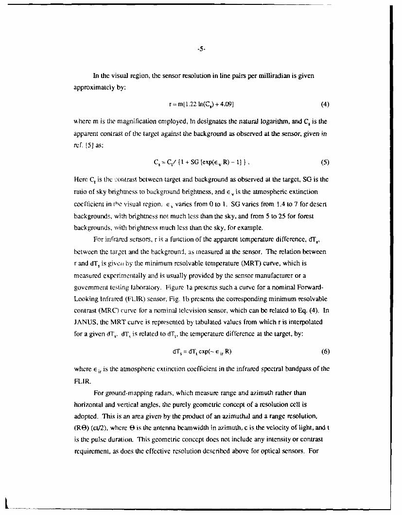
AD-A235 592 A RAND NOTE Suggested Modifications to Optical Sensor Algorithms in JANUS H. H. Bailey, L. G. Mundle, H. A. Ory November 1990 ! ~. . . . . . . ... 91-00342 RAND I 91 5 22 099
| Date post: | 11-Oct-2018 |
| Category: |
Documents |
| Upload: | hoangduong |
| View: | 215 times |
| Download: | 0 times |

AD-A235 592
A RAND NOTE
Suggested Modifications to Optical SensorAlgorithms in JANUS
H. H. Bailey, L. G. Mundle, H. A. Ory
November 1990
! ~. . . . . . . ...
91-00342
RAND I 91 5 22 099

The research described in this report was jointly sponsored by the Director ofDefense Research and Engineering, Contract No. MDA903-90-C-0004; theUnited States Army, Contract No. MDA903-86-C-0059; and the United StatesAir Force, Contract No. F49620-86-C-0008 and was conducted by all three ofRAND's federally funded research and development centers: the NationalDefense Research Institute (Office of the Secretary of Defense, and JointChiefs of Staff); the Arroyo Center (Army); and Project AIR FORCE (AirForce).
The RAND Publication Series: The Report is the principal publication doc-umenting and transmitting RAND's major research findings and final researchreaults. The RAND Note reports other outputs of sponsored research forgeneral distribution. Publications of The RAND Corporation do not neces-sarily reflect the opinions or policies of the sponsors of RAND research.
Published by The RAND Corporation1700 Main Street, P.O. Box 2138, Santa Monica, CA 90406-2138

Unclassified
SECURITY CLASSIFICATION OF THIS PAGE (When Doa Entered) _
R O . ..A PAREAD INSTRUCTIONSREPORT DOCUMENTATION PAGE BEFORE COMPLETING FORM
REOR. NUMBER GOVT ACCESSION NO. 3. RECIPIENT'S CATALOG NUMBER
N-3087-DR&E/A/AF
4. TITLE (end Subtlifle) S. TYPE OF REPORT & PERIOD COVERED
Suggested Modifications to Optical Sensor interimAlgorithms in JANUS
6. PERFORMING ORG. REPORT NUMBER
7. AU THOR(*) S. CONTRACT OR GRANT NUMBER(3)
H. H. Bailey, L. G. Mundie, H. A. Ory MDA903-90-C-0004
9. PERFORMING ORGANIZATION NAME ANO AOORESS i0. PROGRAM ELEMENT. PRIOJECT. TASKAREA a WORK UNIT NUMBERS
The RAND Cornoration
1700 Main Street
Santa Monica, CA 90406
II. CONTROLLING OFFICE NAME ANO AOORESS 12. REPORT DATENovember 1990..
Office of the Under Secretary of Defense
Research and Engineering 13. NUMBEROF PAGES
Washignton, DC 203u1 2514. MONITORING AGENCY NAME & AOORESS(II dllferonrti from Confro llin Office) IS. SECURITY CLASS. (of tAi ,eport)
unclassified1a. OECL ASSI FICATON/OOWN GRAOING
SCHEDULE
16. OISTRIBUTION STATEMENT (*I this Report)
Approved for Public Release; Distribution Unlimited
17. DISTRIBUTION STATEMENT (ai he labtrgact entered in Block 20, It different fIm Reporf)
No Restrictions
,d. SUPPLEMENTARY NOTES
19 K EY WOROS (Continue on reverae sods of necesirn and Identify by block namber)
Target AcquisitionOptical Detectors
Algorithms
Simulation
20 ABSTRACT (Continue on reveree sods It necessry and identily by block number)
see reverse side
DD , JAN ' 1473 Unclassified
SECURITY CLASSIFICATION - PAG * I.- En,.,'YI

Unclassified
SECURITV CLASSIFICATION OF THIS PAGE(Who Do#a Zit.d)*
Optical sensor algorithms in the JANUS(T)ground combat simulation do not include arepeated detection criterion for targetacquisition and weapon firing, nor do theyprovide for the effects of falsedetections. As a result, targets detectedwith very low probability, such as those atranges near the performance limit of thesensor, will often give rise to acquisitionand weapon-firing decisions when raresingle detections result from coverage bymany sensors and time cycles. This Notereviews the detection algorithms foroptical sensors implemented in JANUS(T),identifies some approximations that canlead to overoptimistic estimates of targetacquisition probabilities when thecalculated detection probability is small,and suggests an acquisition criterion thatalleviates the problem.
Unclassified
sCU pIry CLASSIF(CATION Oo ris AG E(w7. ., 00.i

A RAND NOTE N-3087-DR&E/A/AF
Suggested Modifications to Optical SensorAlgorithms in JANUS
H. H. Bailey, L. G. Mundie, H. A. Ory
November 1990
Prepared for theDirector of Defense Research and EngineeringUnited States ArmyUnited States Air Force
RAN D APPROVED FOR PUSUC RELEASE; DISTRIBUTION UNLIMITED

-Ill-
PREFACE
This Note reviews the detection algorithms for optical sensors implemented in the
JANUS(T) engagement model, identifies some approximations that can lead to
overoptimistic estimates of target acquisition probabilities when the calculated detection
probability is small, and suggests an acquisition criterion that alleviates the problem.
Various implementations that differ in the amount of additional computing burden
required are described for the acquisition criterion.
The results should be of interest to anyone involved in applications of the
JANUS(T) engagement model.
The research was carried out as part of the Joint Close Support Study, and this
Note is part of a series of publications documenting that work. The project was jointly
sponsored by the Director of Defense Research and Engineering, the U.S. Army, and the
U.S. Air Force and was conducted by all three of RAND's federally funded research and
development centers (FFRDCs): National Defense Research Institute (Office of the
Secretary of Defense, and Joint Chiefs of Staff); the Arroyo Center (Army); and Project
AIR FORCE (Air Force).
-v-
SUMMARY
The target acquisition algorithms implemented for optical sensors in the
JANUS(T) ground combat simulation, unlike radar sensor algorithms, are found to
include no requirement for repeated detection as a condition for target acquisition
declarations and weapon firing, nor any consideration of possible false detections. As a
result, targets detected with very low probability, such as those at ranges near the
performance limit of the sensor, will often give rise to acquisition and weapon firing
decisions when rare single detections result from coverage by many sensors and time
cycles. A stronger criterion is needed for target acquisition and weapon firing than just a
single detection, to avoid overestimating the number of acquisition and weapon firing
events for long range targets.
An acquisition criterion is suggested, similar to that used with radar sensors in
JANUS, in which two detections out of three successive scans are required to
accomplish acquisition and fire weapons. This criterion is effective primarily in the
region of small detection probability, where the corresponding acquisition probability
approaches a square law dependence on the detection probability. This lowers
acquisition when the detection probability is small and greatly reduces the number of
weapon firings at long range.
Various methods for implementing the acquisition criterion in JANUS have
different effects on the computational load. JANUS is interactive, and it is desirable to
minimize the computing load and execution time. A direct implementation, similar to the
way that radar sensors are currently modeled, stores detection results for two previous
scans, and detection during the current scan is counted as acquisition if detection
also occurred on one of the two previous scans. This implementation involves
specifying search sectors and scan rates for each sensor, accumulating sensor scanning
time over JANUS cycles until it equals the time required for the sensor to cover its
assigned search sector, then evaluating target detection for the completed scan. It thus
requires more computation than the current algorithms and storage of many more
variables, including detection results for two previous scans for each sensor and target
combination. A variation of this approach avoids storage of results by evaluating
acquisition based on the probability of two detections out of three scans as approximated

-vi-
b) repeated application of the results from the current scan to simulate those that would
be obtained from successive scans.
An indirect implementation applies the acquisition criterion to the JANUS
procedure for setting threshold resolution requirements for accessibility of targets to
detection, which otherwise is based on a single detection requirement. The current
JANUS procedure involves drawing a random number between 0 and I and inserting it
into the relationship, expressed in a data table, between sensor resolution and the time-
independent part of the detection probability to determine the threshold resolution
required for accessibility of a given target to detection by a given sensor. The indirect
application of the acquisition criterion involves replacing the current data table by one
that expresses the relationship between sensor resolution and an acquisition probability
expression derived from the time-independent part of the detection probability.
Additional computation and data storage are not required for this indirect approach.
If computing resources permit, the full direct implementation of the acquisition
criterion for optical sensors is recommended. If variable storage must be minimized,
then the variation described for the direct implementation is recommended. If no
additional computing burden can be tolerated, then the indirect implementation is
recommended. Even this indirect approach would greatly improve the modeling of target
acquisition and weapon firing.
-vii-
CONTENTS
PREFACE .. . . . . . .. . . . . . .. . . . . . .. . . . . 1i
SUMMARY ................................................... v
FIGURES AND TABLE........................................... ix
SectionI. INTRODUCTION........................................... I
II. CURRENT IMAGING SENSOR ALGORITHMS......................3Time-Independent Term..................................... 3Time-Dependent Term. ...................................... 7Evaluation Procedure....................................... 8
III. SUGGESTED ACQUISITION CRITERION........................I IRationale...............................................I IDirect Impnlementation...................................... 12Variation on Direct Implementation ........................... 14Indirect Implementation ................................... 17Summary of Implementation Options .......................... 19
IV. CONCLUSIONS ......................................... 23
REFERENCES .............................................. 25
-ix-
FIGURES
1. Examples of sensor resolution performance curves .................. 62. Relationship between detection and acquisition probability based
on a requirement for two detections out of three successive scans ........ 163. Relationship between the time-independent part of the detection
probability and the resolution cycle ratio, C/M ..................... 18
TABLE
1. Threshold resolution requirements for target accessibility .............. 20

-1-
I. INTRODUCTION
Optical sensor algorithms in the version of the JANUS ground combat model
currently in use include no repeated detection criterion for target acquisition and weapon
firing, and no provision for the effects of false detections. A single detection, even
though a rare and isolated event, can result in a weapon firing decision. The probability
of such an event can be appreciable when the detection probability is accumulated from
many sensors over an extended duration. It can lead to an overestimate of sensor and
weapon performance at long ranges. Here we examine whether a repeated detection
criterion is needed as a basis for acqui .ion and weapon firing, what its effects would be,
and how such a criterion could be implemented.
JANUS(T) is an interactive, two-sided, closed, stochastic ground combat
simulation developed and maintained by the U.S. Army Training and Doctrine
(TRADOC) Systems Analysis Activity (TRASANA), which is now called the TRADOC
Analysis Center (TRAC), at White Sands Missile Range, New Mexico. It is derived
from the Lawrence National Laboratory prototype model JANUS. Most air and ground
systems that participate in offensive and defensive operations are represented, with
emphasis on those that participate in maneuver and artillery operations on land. [ I ]
JANUS(T), hereafter referred to simply as JANUS, is widely used for operational
effectiveness analyses, at RAND as well as other locations.
It is characteristic of models that approximations arc involved in the
representation of systems and their performance, and in the overall description of
operations. Because JANUS is interactive, computations must be sufficiently rapid to
allow simulation time not greatly different from real time. Some of the model's
approximations are designed to improve the speed of computation. Usually the
approximations are consistent with the scenario assumptions, but it is always necessary to
examine whether a given scenario produces circumstances in which particular
approximation errors are emphasized that might affect the results significantly.
Consider an example in which ranges between sensors and targets are usually
sufficiently long that detection during any sensor scan is a low probability event, but
many sensors arc involved over many scan periods. The cumulative single detection
probability can become large and can result in weapon firing decisions based on single

-2-
detections. For example, simulation of standoff weapons emphasizes the accuracy of the
detection algorithm in circumstances that may be quite different from those for which it
was derived. As a case in point, algorithms for imaging sensors in JANUS are based on
a detection model that was derived under conditions where det ction probabilities were
much larger than occur during simulations of combat near the range limit 9f the sensors.
During some JANUS simulaiion exercises, target detection and weapon firing
actually were obsern'zd at ranges lorger than expected for the sensors being modeled.
Calculations 5ased on JANUS algorithms also produced small, single-look detection
probabilities, on ,.e order of I percent, at similar long ranges. An appreciable detection
probability, which in JANUS is essentially the acquisition probability, resulted wnen the
small, single-look dcZction probability accumulated over many sensors and time cycles.
With actual sensors, acquisition at small, single-look detection probabilities would
require difficult discrimination against the effects of noise and clutter, which are not
represented in th. JANUS model. However, if noise and clulor effects had been
represented, they might well have given a comparable number of false detections.
Therefore, we investigated possible modifications to the JANUS optical sensor
algorithms that would represent rare detection events more realistically.
This Note examines the representation of imc-ing sensors in the JANUS model
and suggests modifications that would improve the accuracy of target acquisition
calculations in long range combat circumstances. Section II reviews the imaging sensor
detection algorithms and their implementation in JANUS -id identities some of their
limitations. Section III presents modified algorithms with a stronger criterion for target
acquisition and weapon Fring and illustrates their cffec,:ts. Various methods, differing in
the amount of computational burden they impose, are suggested for their implementation
in the JANUS model. Conclusions and recommendations for implcmcnting the
acquisition criterion are summarized in Sec. IV.
-3-
II. CURRENT IMAGING SENSOR ALGORITHMS
The best experimental data on the probability of target acquisition by a human
observer, through direct vision or by observing sensor imagery displayed electronically,
are probably those obtained by the Army's Night Vision Laboratory (NVL), now called
the Center for Night Vision and Electro-Optics (CNVEO), at Ft. Belvoir, Virginia. Their
results have been extended to broader conditions than those of the original experiments
rcported in Johnson's classic paper, 121 and were incorporated into a model that is
usually referred to as the NVL model. [3-41 This model, widely used for analyses of
sensor performance, provides the basis for the representation of imaging sensors in
JANUS. It expresses the detection probability as the product of two terms--P 1 , the
probability of detection with unlimited observation time, which depends primarily on
resolution and contrast, and P2, a time-dependent term that takes account of search
sectors, fields of view, and coverage during a scan time.
TIME-INDEPENDENT TERM
The first term, P1, expresses the experimental observation that, with unlimited
observation time, the probability of detection is a function of C, the number of resolvable
modulation cycles (or line pairs, or resolution cells) present within the critical (usually
minimum) dimension of a target image. The resolution is dependent on sensor quality,
target contrast, and propagation effects. P, is also a function of the background clutter,
type of target, and the kind of decision to be made (detection, recognition, etc.). These
latter factors arc combined into a parameter, M, which scales the resolution requirement;
it is the value of C required to yield a specified value (usually 0.5) for P1, for whatever
types of clutter, target, and decision are specified.
Examples of M can be cited to give a feeling for its magnitude. As noted, the
number of line pairs achieved in resolution must equal M for a 50 percent detection
probability given unlimited observation time. M is often considered to be a fixed scale
value, which, for the example of a small armored vehicle, is set as I for detection against
a reasonably uniform background, 2 for detection in medium clutter, 4 for recognition,
and 6.4 hr idcntification. Actually, M should be thought of as a parameter to which a

-4-
number must be assigned in setting requirements, but for which few guidelines can be
provided. It can be argued that a weapon-firing decision is intermediate between mere
detection and full recognition, and therefore in many cases a value of M = 3 is
appropriate; this perception level is sometimes called classification. The approximate
nature of defining M is implicitly acknowledged by the common use of small integers to
describe a continuous variable.
In the NVL model, P, is represented as a function of the ratio C/M and expressed
by the following empirical equation:
(C/M)2 .7 + .7(C/M)
1 + (C/M)2 "7 + 0.7(C/M)
The expression satisfies the requirement that when C = M, then P = 0.5. The datz to
which this equation is a fit are very approximate. Variability is caused by background
clutter, observer skills, target type, detection criteria, and other factors. Also, it is in the
nature of these empirical data that small departures from zero or unity are difficult to
observe and quantify; therefore, accuracy is probably greatest in the midrange of values.
Other empirical functions can also be used to represent P1. We note in passing that an
expression derived in unpublished work by H. Bailey agrees with the previous expression
more closely (within about 2 percent) than can be easily distinguished by comparison
with the approximate experimental data:
P1 =1 - exp[ - (0.84C/M)2 41 (2)
This form may be more convenient for use in some analyses.
To determine the value of P in a given situation, one must assign a value to M
appropriate to the conditions of the situation and determine the number of resolution
cycles across the minimum target dimension, C, achieved by the sensor under the
prevailing conditions.
For a sensor that resolves only in angle, the resolution is given by the relation:
C=rrO (3)
where r is the resolution of the sensor, usually expressed as the effective number of
resolvable line pairs (sometimes called cycles) per milliradian, and E is the angular
subtense at the sensor, in milliradians, of the critical (usually minimum) dimension L of
the target. For a target at range R, e is simply L/R. The value of r depends on the type
and quality of the sensor.
-5-
In the visual region, the sensor resolution in line pairs per milliradian is given
approximately by:
r = m[ 1.22 ln(C) + 4.091 (4)
where m is the magnification employed, In designates the natural logarithm, and C, is the
apparent contrast of the target against the background as observed at the sensor, given in
ref. f51 as:
Cs = Ct/{1I + SG [exp(E V R) - 1] }.(5)
Here C, is the 2oritrast between target and background as observed at the target, SG is the
ratio of sky brightness to background brightness, and E, is the atmospheric extinction
coefficient in I.Ie visual region. E, varies from 0 to 1. SG varies from 1.4 to 7 for desert
backgrounds, with brightness not much less than the sky, and from 5 to 25 for forest
backgrounds, witlh brightness much less than the sky, for example.
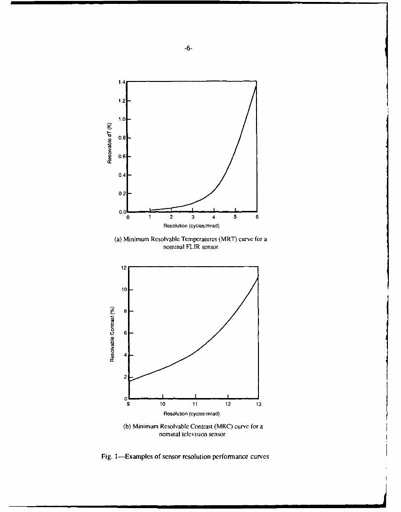
For infrared sensors, r is a function of the apparent temperature difference, dT,,
between the target and the background, as measured at the sensor. The relation between
r and dT, is givci by the minimum resolvable temperature (MRT) curve, which is
measured experimentally and is usually provided by the sensor manufacturer or a
government testing laboratory. Figure Ia presents such a curve for a nominal Forward-
Looking Infrared (FLIR) sensor; Fig. l b presents the corresponding minimum resolvable
contrast (MRC) curve for a nominal television sensor, which can be related to Eq. (4). In
JANUS, the MRT curve is represented by tabulated values from which r is interpolated
for a given dT,. dT, is related to dT t, the temperature difference at the target, by:
dTs = dT t cxp(- E ir R) (6)
where E ir is the atmospheric extinction coefficient in the infrared spectral bandpass of the
FLIR.
For ground-mapping radars, which measure range and azimuth rather than
horizontal and vertical angles, the purely geometric concept of a resolution cell is
adopted. This is an area given by the product of an azimuthal and a range resolution,
(RO) (cl/2), where E is the antenna beamwidth in azimuth, c is the velocity of light, and t
is the pulse duration. This geometric concept does not include any intensity or contrast
requirement, as does the effective resolution described above for optical sensors. For
-6-
1.4
1.2
1.0
S0.8-
0S0.6
0.4
0.2
0.cLI I0 1 2 3 4 5 6
Resolution (cycles/mrad)
(a) Minimum Resolvable Temperatures (MRT) curve for anominal FLUR sensor
12
10
0 6 6
0
8 4Cc
2
0,9 10 11 12 13
Resolution (cycles/mrad)
(b) Minimum Resolvable Contrast (MRC) curve for anominal television sensor
Fig. I-Examples of sensor resolution performance curves
-7-
radars, contrast is replaced by a signal-to-noise or a signal-to-clutter ratio (depending on
which is dominant), and the probability of detection is calculated rigorously for a
specified false detection rate, Pfd. Note that, in the optical imaging case, Pfd is selected
implicitly and subjectively by an observer as he assesses what he considers to be the
effective or usable resolution, whereas for radars this quantity must be entered explicitly.
For optical imaging sensors, it is not known what value is typically selected. It may often
range between 10-3 and 10- 6 depending on the observer's visual acuity, his motivation at
the time, and other factors. In radar calculations, a value at the more conservative end is
commonly used, such as Pfd = 10-6, but not necessarily so.
Considerations up to this point presuppose a line of sight (LOS) between the
sensor and the target. Actually, there may be interferences from terrain or smoke, and
these are handled by the JANUS model. JANUS includes a detailed terrain model that is
used to evaluate whether a line of sight exists between the sensor and the target. An
obscuration factor is incorporated into P1 as a multiplying factor, dependent on the LOS
conditions. Smoke obscuration, which is more dynamic, is addressed in a similar
manner, but the obscuration factor multiplies the time-dependent term.
TIME-DEPENDENT TERM
The time-dependent term in the detection model is given by:
P2 = 1 - exp[ - (C/M) (t/6.8)] (7)
Here t is the amount of time that the target is within the sensor's field of view, termed the
observation time. The C/M factor in the exponent can be thought of as describing the
efficiency with which the observation time can be utilized; greater resolution facilitates
detection. The experimentally determined constant, 6.8, presumably relates to the
number of fixation points within a typical field of view. If one field of view is observed
within the cycle time of 2 sec, at which JANUS operates, the effective amount of time
that the eye fixates on a particular target is 2/6.8 sec, close to the classical fixation
interval or glimpse time of 1/3 sec.
In JANUS, if a total search sector (SS) is to be covered by a sensor with a field of
view (FV) then the time available for looking in each field of view is:
j=2 (FV/SS) (8)
iI__ - I l m m i H ib lIi ii
-8-
where the subscript J indicates that this expression is specialized to the JANUS cycle
time. Substituting this value of t into Eq. (7) yields the expression:
P2j = I - exp[ - (C/M) (2/6.8) (FV/SS)] (9)
where the second subscript again refers to JANUS specialization. As mentioned earlier,
P2j is also multiplied by another factor to account for whether smoke obscures the line of
sight between sensor aid target, but this aspect is peripheral to the present discussion.
EVALUATION PROCEDURE
JANUS is a stochastic model in which outcomes of events are determined by
random draws against their probabilities of occurrence, rather than being described by a
statistical average. Although the model for detection probability has the form of a
product of conditional probabilities, the outcomes of P, and P 2 are evaluated separately
and then multiplied. If the outcome from P, is zero, then no detection is possible, no
matter what the value of P2. If the outcome from P1 is unity, then the outcome from a
random draw against the value of P2 determines whether detection occurs.
Evaluation of P is actually implemented indirectly in JANUS, in a manner that
reduces the amount of computation required. Also, the value of M used to evaluate P1 is
always taken as 3.5 (insofar as the internal data table that is used is constructed using this
value); this value provides sufficient recognition to support a weapon-firing decision; no
other recognition requirement is included in the JANUS model. For each target and
sensor combination, the indirect procedure involves making a random draw against the
range of values of P,, 0 to 1. According to Eq. (1), a given result corresponds to a
particular value of C/M and for the value M = 3.5 used to justify the weapon firing
decision, corresponds to a particular value of C. That value of C is identified as a
threshold value, such that during each cycle time, if the value of C calculated in the
JANUS PAIRS subroutine (based on Eq. (3)) exceeds the threshold, then the given target
is accessible to detection by the given sensor, otherwise it is not. The random draw that
determines the threshold C is performed only once during initialization, and the
thresholds are not changed during a particular JANUS run. This procedure is
implemented in the JANUS INITACQ subroutine, and the data table PAIRSVAL is
entered with the result of the random draw to extract the threshold value of C. Use of
this procedure provides stochastic results while requiring computation of target
-9-
accessibility only once. Thus, it minimizes the computational load and improves the
speed of execution.
P2 is evaluated at each time cycle according to Eq. (9), using particular values of
variables appropriate to the situation at the time and a nominal value of M = 2, which
assumes detection against medium clutter. Some adjustments are applied in particular
cases, such as for a moving target or one that has just fired, but these adjustments are not
germane to the current discussion. In the process, the resolution, C, achieved under
current conditions is evaluated. If the value of C is less than the threshold value, then the
target is not accessible to detection. If the value of C equals or exceeds the threshold
value, then a random draw is made against the value of P2, and the outcome determines
whether the target is detected. If detected, the target is added to the target list for the
sensor (subject to other conditions that can be ignored here), and no furthe det.,idon
criteria must be satisfied to initiate weapon firing.
This procedure is repeated each JANUS time cycle. Assuming for convenience
that P2 maintains a constant value, the average cumulative detection probability for a
given target within the search area of a given sensor over N time cycles is
0 if C < Cthreshold
Pd(N) = (10)
1 -(I P) if C -> Cthreshold
If a given target is within the search area of n sensors over N time cycles, the probability
that Ci >_ Cheshold for any sensor i is P,, and the average number of effective sensors neff
for which Ci _ Chrshold is the sum of the P1, over the n sensors. The cumulative
detection probability for n sensors and N cycles, assuming that P2 remains constant, is
then:
Pd(n,N) I -n -[Pd, (N)] (11)
= - [I - P21Nnff
Of course, P2 does vary, and there are correlations among P1, P2, and C; however, the
above equations illustrate the general dependence of Pd on n and N. The numbers of

sensors and time cycles can be large, so Pd(nN) can grow to an appreciable value, even
for such small values of Pd as might occur near the sensor's range limit.
All the burden of establishing target recognition sufficient for firing is carried byPI, and only a single detection is required to enable tracking and weapon firing.
special criteria are imposed to avoid possible false detections; indeed, JANUS includes
no provisions for false detections or their consequences.
-11-
III. SUGGESTED ACQUISITION CRITERION
RATIONALETarget detection based on a single look is probably not an adequate criterion for
initiating the firing of a weapon. Successive looks at a sensor image of the real world in
real time are not identical, for a wide range of reasons. The target may be moving with
respect to the clutter. The target may be nominally at rest but moving slightly (such as a
hovering helicopter) so that, if the observed contrast is marginal, motion of as little as a
single pixel through the clutter could alter the perceived shape of a target. There may bemotion internal to a target, such as moving guns or rotors, or internal to the clutter, such
as wind-caused foliage movement. The sensor may be moving with similar
consequences. There is always some detector or receiver noise, even though in a well-
designed system these are seldom limiting or even noticeable. There is always somc
electronic noise in a display, which usually is noticeable. The observer's visual system
has its own noise, quantum noise at low light levels, electrical noise in the retina and
tlerves, and changing perception thresholds because of motivation or extraneous inputs.
Illumination and thermal conditions vary. At the margin of barely detectable targets, all
of these phenomena may be operating. One is not looking at a static photograph, and
experienced observers will seldom trust a single glimpse; rare detection must be
confirmed by repetition to be trusted.
Radar engineers and operators concerned with detecting isolated targets (e.g.,
aircraft) at long range (usually limited by receiver noise) have developed an acquisition
criterion of at least two detections out of three successive antenna scans. Indeed, this
criterion is incorporated in the JANUS model for radar sensors. The details are
somewhat different for optical sensors, but a similar criterion of two detections out of
three successive looks is appropriate. Perhaps the criterion should be a slightly different
ratio, such as three out of five, but in general the numerator probably should be greater
than one and the denominator less than ten.
Until better experimental data become available, we suggest addition of anacquisition criterion for optical sensors based on a requirement for two detections out of
three successive scans. This criterion would increase the complexity of the model, so
three possible implementation methods, suggested below, entail different degrees of

-12-
complication. A direct implementation involves storage of detection results from two
previous scans and comparison with the current result; tis is similar to the current radar
algorithms. A variation of this method avoids the storage requirement by computing the
probability that two detections would occur within three successive scans, based on the
result from the current scan. An indirect implementation minimizes modifications to the
JANUS program. No additional variables or computations are required, only substitution
of values derived from a repeated detection requirement for those currently in the
JANUS PAIRSVAL data table mentioned above.
DIRECT IMPLEMENTATION
Direct implementation of the two out of three acquisition algorithm would require
considerable change from the way JANUS currently implements optical sensors.
JANUS evaluates detection by a random draw against the detection probability
calculated for each time cycle, which implicitly assumes a scan rate adequate for sector
coverage within a time cycle. The observation time that is allocated to each target
location may be quite small. Actually, the time required for a sensor to complete a full
scan is usually longer than a single JANUS time cycle. Nevertheless, although it does
not exactly replicate sensor operations, the JANUS procedure linearly approximates the
more exact representation of detection probability, and that is sufficiently accurate as
long as the calculated detection probabilities are small. For larger detection probabilities,
the JANUS procedures somewhat overestimate the detection probability. However, the
linear approximation is often adequate for determination of the single-look detection
probability.
The linear approximation is not adequate for application of the two out of three
acquisition criterion, because this criterion is essentially nonlinear and must be applied to
a complete detection cycle over the full sensor scan period, not just a fragment. To apply
it properly, JANUS procedures must utilize the correct representation of sensor
observation time in the detection equations described earlier. Search subsectors must
also te assigned within JANUS so that when they are covered at the scan rate of the
sensor, the correct amount of time will be spent observing the target. Typically, the total
threat sector could be divided by the number of sensors to determine the search subsector
for an individual sensor. If the number of sensors is large enough, a larger subsector
could be assigned with sectors covered by more than one sensor. Particular assignments

-13-
would depend on particular scenarios but in general should be realistic. The time
required to complete a scan is given by the search subsector divided by the scan rate of
the sensor.
Detection should not be evaluated until a scan is completed for whatever search
sector the sensor covers. That usually takes longer than a JANUS cycle, so that the
observation time entering into the exponential time factor of Eq. (7) is the actual amount
of time the target is within the sensor field of view during the scan.
t= t (FV/SS) = FV/a (12)
where % is the scan time for coverage of the search subsector at the sensor scan rate, a,
and the two are related by % = SS/a. This observation time differs from that in Eq. (8) by
the use oft% rather than the JANUS 2 sec cycle time. Then, if the value of resolution, C,
for the current circumstances exceeds the threshold, a random draw would be made
against the detection probability based on a complete scan, as calculated according to:
P2 = I - e,-p[ - (C/M) (t,/6.8) (FV/SS)] (13)
= I - exp[ - (C/M) (FV/6.8a)]
The result would then be compared with the stored results of earlier detection scans. If
the current scan plus one of the two previous scans achieved detection, then the target
would be acquired. Two flags would be associated with each sensor and target
combination, one flag to store the results for each of the two previous scans, and the flags
set according to detection results as each scan is completed. If a given scan does not
achieve detection, flag settings are shifted backward one scan and compared again in the
next scan.
Some aspects of this model for optical sensors involve license that is not involved
in the corresponding model for radar sensors. The performance of radar hardware is
determined according to operational settings made by the operator. By contrast, optical
sensor scanning rate and sector coverage are often controlled by human observers who
can and do introduce variations in the scanning rate and sector coverage. This can aid or
hinder the search process, according to the circumstances. However, for modeling
purposes, this source of variabili'y is ignored and the optical sensors are assumed to
search in a regular manner that is more amenable to analytical modeling.
-14-
The approach outlined here is a direct implementation of the two out of three
acquisition criterion and is very similar to the procedure currently used in JANUS for
radar sensors. It does increase the number of variables involved in JANUS calculations,
including the two detection flags for each sensor and target combination, the particular
sensor search subsector (which must be redefined each time the sensor moves), the
sensor scan time, and the accumulated search time. Additional computations are
involved in accumulating search time and comparing it with the sensor scan time, and in
comparing results from successive scans; this is somewhat offset by the smaller number
of evaluations of detection probability for each sensor scan time rather than for each
JANUS cycle. Setup effort is increased slightly by the increased number of parameters.
This implementation is recommended if computing resources are available to support it.
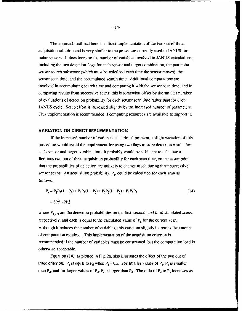
VARIATION ON DIRECT IMPLEMENTATION
If the increased number of variables is a critical problem, a slight variation of this
procedure would avoid the requirement for using two flags to store detection results for
each sensor and target combination. It probably would be sufficient to calculate a
fictitious two out of three acquisition probability for each scan time, on the assumption
that the probabilities of detection are unlikely to change much during three successive
sensor scans. An acquisition probability, -', could be calculated for each scan as
follows:
P = PIP 2 ( - P 3) + PIP3( - P2 ) + P2P 3( - P) + PP 2P 3 (14)
= 3P2-2P21d 2d
where P12,3 are the detection probabilities on the first, second, and third simulated scans,
respectively, and each is equal to the calculated value of Pd for the current scan.
Although it reduces the number of variables, this variation slightly increases the amount
of computation required. This implementation of the acquisition criterion is
recommended if the number of variables must be constrained, but the computation load is
otherwise acceptable.
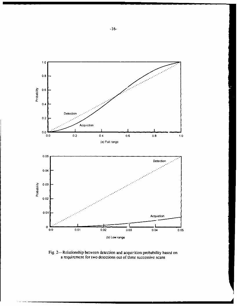
Equation (14), as plotted in Fig. 2a, also illustrates the effect of the two out of
three criterion. P. is equal to Pd when Pd = 0.5. For smaller values of Pd, P. is smaller
than Pd, and for larger values of Pd' P. is larger than Pd. The ratio of Pd to P, increases as
-15-
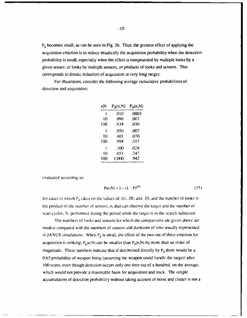
Pd becomes small, as can be seen in Fig. 2b. Thus, the greatest effect of applying the
acquisition criterion is to reduce drastically the acquisition probability when the detection
probability is small, especially when the effect is compounded by multiple looks by a
given sensor, or looks by multiple sensors, or products of looks and sensors. This
corresponds to drastic reduction of acquisition at very long ranges.
For illustration, consider the following average cumulative probabilities of
detection and acquisition:
nN Pd(n,N) P.(n,N)
1 .010 .000310 .096 .003
100 .634 .030
1 .050 .00710 .401 .070
100 .994 .517
1 .100 .02810 .651 .247
100 1.000 .942
evaluated according to:
P(n,N) = 1 - (1 - P)n' (15)
for cases in w hich P,, takes on the values of .01, .05, and. 10, and the number of looks is
the product of the number of sensors, n, that can observe the target and the number of
scan cycles, N, perlormed during the period while the target is in the search subscctor.
The numbers of looks and sensors for which the comparisons are given above arc
modest compared with the numbers of sensors and durations of time usually represented
in JANUS simulations. When Pd is small, the effect of the two out of three criterion for
acquisition is striking; P1(nN) can be smaller than Pd(nN) by more than an order of
magnitude. These numbers indicate that if determined directly by Pd there would be a
0.63 probability of weapon firing (assuming the weapon could handle the target) after
100 scans, even though detection occurs only one time out of a hundred, on the average,
which would not provide a reasonable basis for acquisition and track. The simple
accumulation of detection probability without taking account of noise and clutter is not a
-16-
1.0
0.8
0.4
Detecton0 2
Acquistion
0,0 L0.0 0.2 0.4 0.6 0.8 1.0
(a) Full range
0.05 Detection .**
0.04
.~0.03
-0
0.02
0.01Acquiston
00.0 0.01 0.02 0.03 0.04 0.05
(b) Low range
Fig. 2-Rlationship between detection and acquirition probability based ona requirement for two detections out of three successive scans

-17-
reasonable representation of acquisition, tracking, and firing processes. If the two out of
three acquisition criterion is applied, which has an effect equivalent to discrimination
against noise and clutter, the probability of weapon firing is only 0.03, a twenty-fold
reduction.
Direct implementation of the two out of three criterion would require rewriting
parts of the JANUS program. The general logical approach currently used for radar
sensors could bc followed, with different equations used to represent the optical sensors
and minor differences associated with factors specific to optical sensors, such as smoke,
weapon firing, etc. Although the required program changes appear to be minor, they
must also accommodate the logic and interactions associated with various other
subroutines. Further, any changes would also require corresponding changes to the
JANUS support program used to initialize a JANUS scenario and that used for program
maintenance. Although not difficult, the task would also not be trivial.
INDIRECT IMPLEMENTATION
An alternative indirect implementation method is possible that would apply the
acquisition criterion in a limited way, while not increasing the number of variables or
adding to the amount of computation in JANUS. The acquisition criterion could be
applied to the time-independent part of the expression for detection probability, similar to
the way JANUS currently implements the requirement for a weapon-firing decision. One
could detcrmiinc the threshold value of C for each combination of sensor and target by
first obtaining a value from a random draw between 0 and 1, then applying the result
against the relationship betwecn P, (rather than Pid ) and C/M, where Pid is the same as
P, given by Eq. (1) and P1, is derived from Pid according to the relationship expressed in
Eq. (14). The resulting threshold C/M and corresponding threshold C (retaining the
value of M = 3.5) would be that required for acquisition according to the two out of three
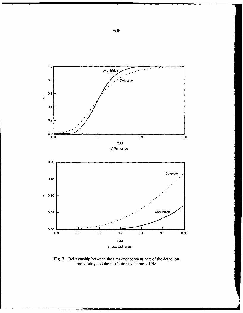
criterion rather than for simple detection. These relationships are illustrated in Fig. 3;
Fig. 3a covers the full range, and Fig. 3b shows an expanded portion for the lower range
between 0.0 and 0.2, of Pid and P1,. In the midrange of values, there is very little
difference in the curves for Pid and P1 ,. and they intersect when (C/M) = 1. For very low
values of P, the values of C/M that correspond to P1, are greater by a large factor than
the values of C/M that correspond to PId- In these cases, the acquisition criterion sets
much larger threshold C values than does the simple detection criterion, and these are
-18-
1.0 Acquisition . .
0-8 .Detection
0.6
0.2
0.010.0 1.0 2.0 3.0
C/M
(a) Full range
0.20
Detection0.15
S0. 10
0.05 .Acquisition
0.00
0.0 0.1 0.2 0.3 0.4 0.5 0.06
C/M
(b) Low CM range
Fig. 3-Relationship between the time-independent part of the detectionprobability and the resolution cycle ratio, C1?NI
-19-
much more difficult to satisfy for targets at long range. Thus, long range targets are
much less likely to be evaluated as accessible to detection and acquisition according to
the acquisition criterion. The more stringent criterion greatly reduces the number of
effective sensors for long range targets. Also, for targets that are evaluated as
inaccessible, compounding of detection probability over large numbers of cycles has no
effect; the targets remain inaccessible and undetected.
The indirect implementation does not apply the full force of the acquisition
criterion; nevertheless, it should greatly reduce the occurrences of acquisition and
weapon firing for targets with low detection probability, such as at long range.
Implementation in JANUS requires only the replacement in the PAIRSVAL table of the
current threshold values of C based on the relationship between Pid and C with new
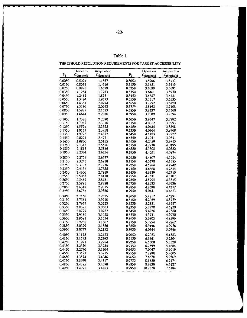
threshold values of C based on the relationship between P1. and C. Table 1 presents
values of Ch,,shojd based on the acquisition criterion that are appropriate for inclusion in
the JANUS model; values of Cthrehld based on Eq. (1), as currently used in JANUS, are
also shown for comparison. In both cases, the value of M = 3.5 is used to scale from
C/M to Cthrshold. Use of the threshold C values based on the acquisition criterion in the
JANUS PAIRSVAL table is recommended if it is necessary to accommodate limited
computing resources.
SUMMARY OF IMPLEMENTATION OPTIONS
The essential modification requirements for the various implementations of the
two detections out of three scans acquisition criterion are summarized below.
Direct Implementation
The direct implementation method provides the full effect of the acquisition
criterion. The modifications required to JANUS include:
1. Specify search subsectors for each sensor and update them after each
movement of target or sensor and specify a corresponding scan time based
on the sensor scan rate.
2. Define and initialize to zero two flags for each sensor and target
combination. One flag is set if target detection occurred in the previous scan,
and the other if target detection occurred in the next previous scan. After
-20-
Table I
THRESHOLD RESOLUTION REQUIREMENTS FOR TARGET ACCESSIBILITY
Detection Acquisition Detection AcquisitionP1 Cthreshold Cthreshold P1 Cthreshold Ctheshold
0.0050 0.5021 1.1557 0.5050 3.5206 3.51370.0150 0.8076 1.4916 0.5150 3.5621 3.54130.0250 0.9870 1.6579 0.5250 3.6039 3.56910.0350 1.1254 1.7783 0.5350 3.6461 3.59700.0450 1.2412 1.8751 0.5450 3.6887 3.62510.0550 1.3424 1.9573 0.5550 3.7317 3.65350.0650 1.4331 2.0294 0.5650 3.7752 3.68200.0750 1.5160 2.0942 0.5750 3.8192 3.71080.0850 1.5927 2.1533 U.5850 3.8637 3.74000.0950 1.6644 2.2080 0.5950 3.9089 3.76940.1050 1.7320 2 2390 0.6050 3.9547 3.79920.1150 1.7962 2.3070 0.6150 4.0012 3.82930.1250 1.8574 2.3525 0.6250 4.0484 3.85980.1350 1.9161 2.3958 0.6350 4.0964 3.89080.1 150 1.9726 2.4?72 0.6450 4.1453 3.92220.1550 2.0271 2.4771 0.6550 4.1951 3.95410.1650 2,0800 2.5155 0.6650 4.2459 3.98650.1750 2.1313 2.5526 0.6750 4.2978 4.01950.1850 2.1813 2.5886 0.6850 4.3508 4.05320.1950 2.2301 2.6236 0.6950 4.4051 4.08740.2050 2.2779 2,6577 0.7050 4.4607 4.12240.2150 2.3246 2.6910 0.7150 4.5178 4.15830.2250 2.3705 2.7236 0.7250 4.5764 4.19490.2350 2.4156 2.7555 0.7350 4.6368 4.23250.2450 2.4600 2.7869 0.7450 4.6989 4.27100.2550 2.5038 2.8178 0.7550 4.7631 4.31070.2650 2.5469 2.8481 0.7650 4.8295 4.35150.2750 2.5896 2.8780 0.7750 4.8983 4.39360.2850 2.6318 2.9075 0.7850 4.9698 4.43720.2950 2.6736 2.9366 0.7950 5.0441 4.48230.3050 2.7150 2.9655 0.8050 5.1217 4.52910.3150 2.7561 2.9940 0.8150 5.2029 4.57790.3250 2.7969 3.0223 0.S250 5.2881 4.62870.3350 2.8375 3.0503 0.8350 5.3778 4.68200.3450 2.8779 3 0782 0.8450 5.4726 4.73800.3550 2.9180 3.1058 0.8550 5.5731 4.79700.3650 2.9581 3.1334 0.8650 5.6805 4.85960.3750 2.9980 3.1607 0.8750 5.7954 4.92620.3850 3.0379 3.1880 0.8850 5.9196 4.99760.3950 3.0777 3.2152 0.8950 6.0544 5.07460.4050 3.1175 3.2423 0.9050 6.2023 5.15830.4150 3.1573 3.2693 0.9150 6.3661 5.25040.4250 3.1971 3.2964 0.9250 6.5500 5.35280.4350 3.2370 3.3234 0.9350 6.7599 5.46840.4450 3.2770 3.3504 0.9450 7.0047 5.60190.4550 3.3171 3.3775 0.9550 7.2988 5.76050.4650 3.3574 3.4046 0.9650 7.6678 5.95690.4750 3.3979 3.4317 0.9750 8.1650 6.21740.4850 3.4385 3.4590 0.9850 8.9330 6.61270.4950 3.4795 3.4863 0.9950 10.9370 7.6184

-21-
each scan, the detection result is placed into the flag for the previous scan,
and previous contents of that flag are shifted to the flag for the next previous
scan.
3. Specify and initialize a timer for each sensor, use it to accumulate time over
JANUS cycles, and compare its contents with the scan time for the sensor.
When the timer contents equal the scan time, reset the timer to zero and
evaluate the detection probability according to Eq. (13) and the requirement
that C exceed CLeshd. If the detection probability is nonzero, draw against
it to determine whether the target is detected. If the target is detected, test to
determine whether it was detected in either of the two previous scans. If so,
consider the target acquired and post it to the sensor target list if the other
conditions are satisfied. If not, shift the contents of detection flags backward
one scan and continue.
Variation of Direct Implementation
The variation on the direct implementation provides essentially the full effect of
the acquisition criterion. The modifications required to JANUS include:
1. Specify search subsectors for each sensor and update after movement, and
specify a corresponding scan time based on the sensor scan rate.
2. Specify and initialize a timer for each sensor, use it to accumulate time over
JANUS cycles, and compare its contents with the scan time for the sensor.
When the timer contents equal the scan time, reset the timer to zero and
evaluate the detection probability according to Eq. (13) and the requirement
that C exceed Cth,,hd. If the detection probability is nonzero, then compute
the acquisition probability according to Eq. (14), and draw against the result
to determine whether the target is acquired. If so, post it to the sensor target
list if other conditions are satisfied. If not, continue.
Indirect Implementation
The indirect implementation provides a large portion of the effect of the
acquisition criterion. The modifications required to JANUS include only:

-22-
1. Replace the values of Cthshld in the PAIRSVAL data table with Ch.hod
values taken from Table 1.

-23-
IV. CONCLUSIONS
The target detection algorithms implemented in the JANUS model for optical
sensors include only weak acquisition requirements, and there is no provision against
false detections, which are ignored. This permits unrealistic acquisition of targets at very
long ranges, based on low detection probabilities, especially when the detection
probabilities are compounded over a long search time or a large number of sensors. As a
result, firing decisions may be made on the basis of rare single detections. Such effects at
long ranges might be emphasized, for example, in simulation of standoff weapons. A
stronger requirement based on repeated detections, such as for two detections out of
three successive scans, would primarily lessen excessively long range acquisitions and
weapon firings.
The acquisition criterion could be implemented by one of the methods described
in Sec. III, selected according to the computing resources available:
I. If sufficient computing resources are available, direct implementation of the
acquisition criterion is recommended. This would apply the acquisition
criterion most strongly and would correspond closely to the way JANUS
currently implements radar sensors.
2. If available computing resources cannot accommodate the number of
variables associated with the direct implementation, then the variation that
approximates the acquisition probability based on only the current detection
probability would be nearly as strong as the full direct implementation.
3. If computing resources are severely constrained, the indirect implementation,
which imposes the acquisition criterion only on the threshold resolution
requirement, is recommended. To accomplish this, the data presented in
Table 1 for the threshold C based on the acquisition criterion can be used to
replace the current values in the PAIRSVAL table that are based on the
single detection criterion. This approach would require minimum effort and,
despite its simplicity, would still to a large extent accomplish the objectives
of the acquisition criterion.
-25-
REFERENCES
1. JANUS(T) Documentation, U.S. Army TRADOC Analysis Center, White SandsMissile Range, New Mexico, June 1986.
2. J. Johnson, "Analysis of Image Forming Systems," Proceedings of Image Intensifier
Symposium, U.S. Army Engineer Research and Development Laboratories, Fort
Belvoir, Virginia, October, 1958.
3. J. A. Ratches et al., Night Vision Laboratory Static Performance Model for Thermal
Viewing Systems, Report 7043, U.S. Army Electronics Command, April 1975.
4. J. A. Ratches, "Static Performance Model for Thermal Imaging Systems," Optical
Engineering, Vol. 15, 525-530, November-December 1976.
5. W. E. Middleton, Vision Through the Atmosphere, University of Toronto Press,
Toronto, 1952.


