A Rational Expectations Modelof Financial Contagion

Laura E. Kodresand

Matthew Pritsker∗

This Version: April 19, 2001Forthcoming in the Journal of Finance

Abstract

We develop a multiple asset rational expectations model of asset prices to explainfinancial market contagion. Although the model allows contagion through several chan-nels, our focus is on contagion through cross-market rebalancing. Through this channel,investors transmit idiosyncratic shocks from one market to others by adjusting theirportfolios’ exposures to shared macroeconomic risks. The pattern and severity of finan-cial contagion depends on markets’ sensitivities to shared macroeconomic risk factors,and on the amount of information asymmetry in each market. The model can gener-ate contagion in the absence of news, and between markets that do not directly sharemacroeconomic risks.

∗International Monetary Fund and the Board of Governors of the Federal Reserve System, respectively.The authors thank Sriram Rajan for research assistance, and Mico Loretan for useful comments and exten-sive guidance in preparing this document. Comments from audiences and discussants at the Federal ReserveBoard, the Bank of Japan, the Federal Reserve Bank of Atlanta Financial Markets Conference, the Interna-tional Monetary Fund, the National Bureau of Economics Research Summer Institute, the Washington AreaFinance Conference, the University of Maryland, Georgetown University, Rutgers University, and VanderbiltUniversity are gratefully acknowledged. The views expressed in this paper are those of the authors but notnecessarily those of the International Monetary Fund or the Board of Governors of the Federal ReserveSystem.

Introduction

A spate of recent financial crises—the Mexican crisis of 1995, the Asian crisis of 1997–98,

the default of the Russian government in August 1998, the sharp depreciation of the real in

Brazil in 1999—have been accompanied by episodes of financial markets contagion in which

many countries have experienced increases in the volatility and comovement of their financial

asset markets on a day-to-day basis. The pattern of contagion has been uneven across both

time and countries—with increased volatility and comovement occurring principally during

times of financial and exchange rate crises—and with some countries, particularly those with

emerging financial markets, having experienced the bulk of the contagion, while countries

with more developed markets have remained relatively unscathed.

Although heightened financial market volatility is to be expected within countries experi-

encing financial and exchange rate crises, the pattern of comovement across countries is not

easily explained. Some of the increased comovement among countries that compete through

trade or share close economic links can be rationalized on the basis of macroeconomic theory;

but these theories are less persuasive in accounting for the increased comovement among the

financial markets of weakly linked countries such as those of South East Asia and Latin

America. An alternative reason for the increased comovement is that financial markets are

responding to the same public news events. However, even accounting for the release of eco-

nomic news and other information, much of the increased volatility and comovement across

countries remains unexplained (Kaminsky and Schmukler, 1999; Baig and Goldfajn, 1999;

Connolly and Wang, 2000).

In this paper we present a rational expectations model of financial markets. The model

is designed to describe asset price movements over short periods of time—such as a day or

a week—during which macroeconomic conditions can be taken as given. Using the model

we provide an explanation for the cross-sectional and time-series pattern of financial market

contagion. In particular we show why emerging markets are especially vulnerable to conta-

gion and why contagion is more likely to appear during times of financial and exchange rate

1

crises. Our model also illustrates how contagion can occur in the absence of public news,

and between countries that do not directly share common macroeconomic fundamentals.

Our paper is related to the burgeoning literature on contagion. One branch of this lit-

erature emphasizes contagious currency crises, relating such crises to various monetary and

financial sector vulnerabilities, including financial market imperfections, incomplete con-

tracting, or weaknesses in government policy. These studies often look for the underlying

causes behind a simultaneous set of speculative attacks.1 A second branch emphasizes con-

tagion spreading as a result of linkages among financial institutions,2 while a third branch

focuses on contagion among financial markets.

Our paper is most closely related to studies of contagion among financial markets. These

papers have principally focused on contagion through a correlated information or a correlated

liquidity shock channel. Under the correlated information channel, price changes in one

market are perceived as having implications for the values of assets in other markets, causing

their prices to change as well (King and Wadhwani, 1990). The correlated liquidity shock

channel posits that when some market participants need to liquidate some of their assets to

obtain cash, perhaps due to a call for additional collateral, they choose to liquidate assets

in a number of markets, effectively transmitting the shock (Calvo, 1999 and Yuan, 2000).

Neither of these channels can completely account for the cross-sectional pattern of conta-

gion. The correlated information channel assumption that price changes in one market have

implications for asset values in other markets is plausible for closely linked markets, but it

seems less reasonable when applied to Latin America and Asia. The correlated liquidity

shock channel is not wholly satisfying for a different reason. Market participants, when hit

with a liquidity shock, would benefit most from selling in highly liquid markets since this low-

ers the impact of their sell orders on prices. This means participants, given a choice—when

1The financial fragilities associated with contagion are analyzed in Corsetti, Pesenti, and Roubini (1999),Rigobon (1998), Agenor and Aizenman (1998), Goldfajn and Valdes (1997), Caballero and Krishnamurthy(1999), Chan-Lau and Chen (1998), Kaminsky and Reinhart (2000) and others.

2Allen and Gale (2000) and Lagunoff and Schreft (2001) provide analyses of contagion caused by linkagesamong financial intermediaries. Van Rijckeghem and Weder (2000) empirically document such linkages.

2

hit with a liquidity shock—would liquidate positions in developed not emerging markets.3

Under this scenario, the fact that contagion has primarily affected a large cross-section of

emerging markets cannot be explained by liquidity shocks alone.

The general model of contagion that we present in the next section is an extension of the

static, single risky asset, noisy rational expectations model of Grossman and Stiglitz (1980),

GS hereafter, to a multiple asset setting. The GS model was first extended to a multiple-

asset setting by Admati (1985) and has since been extended in a number of directions by

others.4 We have stayed close to GS’s original framework to highlight our ideas in as simple

a setting as possible. The main innovation is the economic interpretation that we give to

elements of the GS model. In our model, each risky asset is the national stock market

index of a separate country. The liquidation value of each market index is decomposed into

a component which represents some investors’ private information about that country and

into a residual component which is driven by macroeconomic factors. This decomposition

provides insight into how the macroeconomic risk factor structure of the economy and the

amounts of information asymmetry in different countries together interact to determine the

pattern of financial market contagion.

Our theoretical model nests a number of formal channels for contagion including the

correlated information and correlated liquidity shock channels discussed above. Because

our model is tractable (even with a large number of markets) it can be used to study the

properties of the contagion channels proposed by others. In a recent paper, Kyle and Xiong

(2001) present a model in which contagion only occurs through wealth effects. Because our

model does not contain wealth effects, we view their approach as complementary.

3However, if some money managers are only permitted to take positions in emerging markets and areforced to liquidate their holdings the impact could be concentrated predominately in emerging markets,rather than transferred to the more liquid developed markets. Moveover, there may be instances whereportfolio risk management rules require liquidation in the most risky markets, not necessarily those with themost liquidity (Schinasi and Smith (2000)).

4Admati (1985) considers a continuum of investors that have diverse private information. Others haveextended the model to a dynamic setting with either a single risky asset (Wang, 1993 and 1994) or withmultiple risky assets (Zhou, 1998, and Brennan and Cao, 1997). A recent extension by Yuan (2000) introducesborrowing constraints on the informed investors in a static, single-risky asset setting.

3

Although we believe other channels may be important for contagion, in most of our

analysis here, we concentrate on a variant of the model that only allows for contagion through

a new channel that we refer to as cross-market rebalancing.5 In the cross-market rebalancing

variant of our model investors respond to shocks in one market by optimally readjusting

their portfolios in other markets, transmitting the shocks, and generating contagion. When

portfolio rebalancing occurs in markets with information asymmetries, the resulting price

movements are exaggerated because the orderflow is misconstrued as being information-

based. We believe that the cross-market rebalancing channel has been overlooked in previous

studies and provides a richer explanation of financial market contagion.

We define contagion in our model quite generally as a price movement in one market

resulting from a shock in another market. While this definition is broad, we show that the

price movements resulting from contagion in the cross-market rebalancing variant of our

model are excessive relative to full information fundamentals. Thus, the model generates

price changes that are consistent with the more traditional notions of contagion. However,

despite the connotation that the contagion is “ irrational,” the contagious price movements

generated by our model occur in a framework in which all market participants are rational.

The next section presents our general model of asset prices. The properties of the model

for contagion are explored in sections II through V. Section VI relates the properties of the

model to the patterns of contagion in recent crises. Section VII concludes.

I The General Model

Our model of asset prices is a two period endowment economy. The economy contains N risky

assets with fixed net supply XT , and a riskless asset (the numeraire) which is in perfectly

elastic supply and has a gross rate of return normalized to 1. Investors trade the assets of

the economy in the first period, and then consume the liquidation value of all assets in the

5Fleming, Kirby, and Ostdiek (1998) used the cross-market rebalancing channel as motivation for theirempirical study of volatility comovement. They did not, however, develop a theoretical model.

4

second period. The prices at which trades take place in the first period is denoted by the

N × 1 vector P . The liquidation value of the assets at time 2 is represented by the random

vector v.

A Market Participants

There are three types of participants in the model, informed investors, uninformed investors,

and noise traders (also often referred to as liquidity traders). Informed investors have superior

information relative to other investors about the liquidation value of the assets. They receive

information on the liquidation value of the assets before trading takes place at time 1. Their

information can be represented by decomposing the liquidation value of the assets into two

components, θ and u:

v = θ + u. (1)

The first component, θ, represents the expected value of v conditional on the information

of the informed investors. Throughout the paper we refer to θ as the information of the

informed investors. The second component, u, is a residual which represents that component

of v which is not explained by the information. Because u is a residual, its mean is assumed

to be 0 and it is uncorrelated with θ. The unconditional joint distribution of θ and u is

assumed to be normal with probability distribution

θ

u

∼ N

θ

0

,

Σθ 0

0 Σu

. (2)

Investors in the model are assumed to behave competitively in the sense that they take

prices as given. The number of informed investors is µI and the number of uninformed

investors is µUI . Both types of investors choose their portfolio positions at time 1 to maximize

the expected utility of consuming their time 2 wealth, W2. Informed investors know the

5

realization of θ, and use this information in their portfolio choices. Each informed investor

has CARA utility with risk tolerance parameter τ , and time 1 wealth W1. Borrowing and

lending take place without constraint at the riskless rate of interest, which is normalized

to 0. This allows each informed trader to choose his positions in the risky assets, XI(P, θ),

to maximize:

E[− exp(−W2/τ) | θ] (3)

subject to W2 = W1 + X ′I(v − P ).

It is well known that the optimal choice of XI(P, θ) satisfies:

XI(P, θ) = τ Var(v | θ)−1(E(v | θ)− P )

= τΣ−1u (θ − P ), (4)

where Var(v | θ) = Σu and E(v | θ) = θ. Uninformed investors have the same utility function

as informed investors but choose their portfolio positions without knowledge of θ. They do,

however, know the structure of the model including the unconditional distribution of θ and u

from equation (2). They also observe P (which reveals information about the value of θ) and

condition their choices on P . In particular, the uninformed choose XUI(P ) (the subscript

“UI” denotes “uninformed”), their positions in the risky assets to maximize

E[− exp(−W2/τ) | P ] (5)

subject to W2 = W1 + X ′UI(v − P ).

It is well known that the optimal XUI(P ) satisfies:

XUI(P ) = τ Var(v | P )−1(E(v | P )− P ). (6)

6

The optimal XUI(P ) depends on Var(v | P ) and E(v | P ), and both of these depend on the

informativeness of P for v. These belief functions and P need to be solved together as part

of the overall general equilibrium of the model.

The third type of participants are noise traders. Unlike the first two types of participants

whose demands depend on traders’ assessment of fundamental value, v, noise traders buy

and sell assets based on their own idiosyncratic need for liquidity. The demands of noise

traders are assumed to be uncorrelated with other participants’ objectives, and uncorrelated

with the fundamental value of the assets. The presence of noise traders in our model prevents

equilibrium prices from fully revealing the information of the informed investors. The net

demand of noise traders is denoted by ε, which has the distribution

ε ∼ N (0, Σε). (7)

B Equilibrium and the Information about v Revealed by P

In this section we solve for the competitive rational expectations general equilibrium price

function for the economy. A competitive rational expectations equilibrium exists in period 1

provided that prices P are set so that markets clear, agents are price takers and their demands

maximize their utility, and agents equilibrium beliefs about fundamentals are consistent with

the information about fundamentals that is revealed by prices. We use the market clearing

and belief consistency condition to solve for equilibrium prices and beliefs following a three-

step procedure. First, we substitute the utility maximizing demands from equations (4), (6),

and (7) into the market clearing condition to solve for the information revealed by P given

equilibrium beliefs. Next, we solve for the equilibrium beliefs that are consistent with the

information revealed by equilibrium prices. Finally, given the information revealed by P , we

solve for the equilibrium price function.

Market clearing requires that prices are set so that supply equals demand. This requires

7

that prices P and beliefs E(v | P ) and Var(v | P ) satisfy the equation

XT = µUIXUI(P ) + µIXI(θ, P ) + ε

= µUIτ Var(v | P )−1(E(v | P )− P

)+ µIτΣ−1

u (θ − P ) + ε. (8)

Recall that we assume that uninformed investors know the structure of the model. By

this we mean that they know: the parameters of the demand for assets by the other two

types of investors given in equations (4) and (7); the unconditional distribution of θ and u

given in equation (2); and prices, P . However, they do not know the realization of θ and ε.

Given this information structure, equation (8) can be arranged so that everything known by

uninformed investors is summarized by S(P ), which can be written as θ plus a function of

noise traders’ demands. In other words, knowledge of S(P ) provides uninformed investors

with a noisy signal of θ, the information of the informed investors:

S(P ) = θ +Σuε

τµI, (9)

where

S(P ) =−1

τµIΣu

[µUIτ Var(v | P )−1(E(v | P )− P )− µIτΣ−1

u P −XT

]. (10)

Equation (9) summarizes the information that is revealed by prices to uninformed in-

vestors given their beliefs and knowledge of the economic structure. To make the beliefs

consistent with the information revealed by prices we require that beliefs satisfy the consis-

tency conditions

E(v | P ) = E[v | S(P )] (11)

and Var(v | P ) = Var[v | S(P )]. (12)

8

Imposing these consistency conditions, while exploiting the joint normality of S(P ), θ

and ε, we solve for E(v | P ) as a function of θ and ε, and we solve for Var(v | P ). It is

important to emphasize that our expressions for E(v | P ) and Var(v | P ) are not explicit

functions of equilibrium prices, but are instead consistency conditions on beliefs that must

be satisfied by the equilibrium price function. Equilibrium price functions are found by

rewriting the market clearing condition, equation (8), while substituting in our expressions

for E(v | P ) and Var(v | P ). We also solve for the unconditional variance-covariance matrix

of prices. Our closed-form expression for price is provided in the following proposition:

Proposition 1 The rational expectations equilibrium price function P for the model de-

scribed by equations (1),(2),(4),(6), and (7) is

P = M0 + M1 E(v | P ) + M2 θ + M3 ε (13)

Proof: See the appendix.

This expression for the equilibrium price allows us to characterize how shocks which affect

some assets spread to others. This is analyzed in detail in the next section of the paper.

II Contagion in the General Model

In this section, we derive the channels for contagion that are present in our model. Because

the specification of the assets has been general up to this point, the model can be used to

explain how shocks to one asset or class of assets spread to others. For our purposes, we

interpret each risky asset as representing the portfolio of assets that trade in a particular

asset market, and then use the model to explain contagion between markets. Contagion

occurs when a shock in one market affects prices in other markets. The model contains two

types of shocks, which we refer to as information shocks and liquidity shocks. Information

shocks are the information learned by informed investors, represented by the realizations of

9

θ. Liquidity shocks are the trades made by noise traders due to their idiosyncratic needs

for liquidity, represented by the realizations of ε. To examine how contagion occurs in our

model, we begin by examining the effects that both types of shocks have on prices in general,

and then discuss the circumstances under which the shocks are transmitted across markets.

The relationship between asset prices and various shocks is based on the closed form

expression for P , equation (13). Differentiating P with respect to ε and θ, respectively, the

change in price due to liquidity shocks (noise trading) is

∂P

∂ε= M1

∂ E(v | P )

∂ε+ M3, (14)

and the change in price due to information shocks is

∂P

∂θ= M1

∂ E(v | P )

∂θ+ M2. (15)

The right hand sides of (14) and (15) decompose the effects of a liquidity and information

shock on prices into two components. The first component is the price change that occurs

because the shock changes E(v | P ). We refer to this as the “expectations component” of the

price change because it measures that part of the price change which is due to revisions in the

expectations of uninformed investors. We refer to the second component of the price change

as the “portfolio balance component” because it measures how prices would respond to the

shift in the excess demand curve for assets caused by the shocks if the uninformed investors

believed that the shocks contained no information. It is important to emphasize that the

expressions in equations (14) and (15) are matrices which summarize the sensitivity of prices

to the shocks. Because prices are a linear function of the shocks (see appendix A) the total

price response to a shock is the price sensitivity multiplied by the shock. For example, if

there are more than three markets, then market 3’s total price sensitivity to a liquidity shock

in market 1 is the row 3, column 1 element of ∂P/∂ε; and the expectations and portfolio

balance components of the total sensitivity are the [3, 1] elements of M1∂ E(v | P )/∂ε and

10

M3, respectively. The relative importance of these components will be discussed shortly.

Before studying these components, it is useful to establish the general conditions for the

existence of contagion. An immediate implication of our definition of contagion (as shocks

in one market affecting prices in other markets) is that contagion cannot occur if ∂P/∂ε

and ∂P/∂θ are both diagonal matrices. Whether or not there is contagion, and the relative

importance of the expectations and portfolio balance components, depends on the numbers

of informed and uninformed investors and on other elements of the economic environment.

A Contagion and The Number of Informed and Uninformed In-

vestors

To understand the role that the number of informed and uninformed investors have for

contagion it is useful to consider some limiting cases of our model. For the first limiting

case we hold the number of uninformed investors fixed, but let the number of informed

investors approach infinity. The result is that informed investors push asset prices toward

their expected liquidation values in all markets, and hence there is no contagion. The

economic intuition for this case is provided by the first order condition for informed investors’

optimal portfolio choices. The first order condition requires risky assets to be priced so that,

conditional on the informed investors’ information, the assets earn the riskless rate of return

plus a premium to compensate the investors for risk. Because the riskless rate is normalized

to 0, the first order condition requires risky asset prices to equal the expected value of

v conditional on their information, θ, plus a risk premium. As the number of informed

investors approaches infinity, the amount of risky asset each holds goes to 0; this forces the

equilibrium risk premium to 0 and causes P to converge to θ. Using this limiting expression

for P , one can see that ∂P/∂θ = I and ∂P/∂ε = 0. Since both of these are diagonal there is

no contagion. In our simulation results (section III.B) we find that when more than 5% of

the investors are informed, they drive prices towards fundamentals in all markets, and the

amount of contagion becomes small. Gennotte and Leland (1990) and Admati (1985) also

11

find that when there is more than a small proportion of informed investors, prices closely

reflect fundamentals.

The second limiting case holds the number of uninformed investors fixed and allows the

number of informed investors to approach 0. As the number of informed investors goes to

0, prices only convey public information. This occurs because E(v | P ) converges to its

expected unconditional value, θ. Since this unconditional expected value does not depend

on θ or ε, shocks do not affect expected asset values, and hence the entire price effect of

shocks occurs through the portfolio balance component.

The third limiting case holds the number of informed investors fixed, but lets the number

of uninformed investors approach infinity. The result is that the risk premium that unin-

formed investors earn for holding the risky assets goes to zero, and hence prices converge

to E(v | P ), the expected liquidation value of the assets conditional on the uninformed in-

vestors’ information. In this limiting case, the price effect of shocks occurs only through the

expectations component.

The second and third limiting cases are of particular interest because both approximate

the realistic situation that the fraction of informed investors is small, but they reach opposite

conclusions about the relative size of the portfolio balance and expectations components of

price changes. This shows that the fraction of informed investors alone does not restrict the

relative importance of the two components. Other elements of the economic environment,

however, do affect their relative importance. We will return to this topic in section III.B

below, after examining the role of the economic environment in determining the channels for

contagion.

B The Economic Environment and the Channels for Contagion

In this subsection, to identify the channels for contagion, we first establish a set of conditions

which are sufficient to ensure that there is no contagion between any markets.

12

Proposition 2 If Σθ, Σu, and Σε are all diagonal matrices, then there is no contagion from

any market to any other market.

Proof: See the appendix.

The intuition behind proposition 2 is that the conditions of the proposition rule out all

channels through which a change in price in one market can have an effect on asset demands

in another market. There are three general ways in which changes in price in one market

can affect demand in other markets. The first two are the standard income and substitution

effects from the Slutsky equation. The third is an information effect in which price changes

in one market potentially reveal information about asset values in other markets.

Income effects are never present in our model due to our assumption that investors have

CARA utility and are unrestricted in their ability to borrow. An additional consequence

of our CARA utility assumption, combined with our assumption that liquidation values

are normally distributed, is that risky assets are substitutes for each other only if their

liquidation values are correlated. Proposition 2 restricts Σθ and Σu to be diagonal, which

forces liquidation values to be uncorrelated and hence rules out substitution effects.

Information effects in the model can occur in two ways. The first is if the informed traders’

information is correlated across markets. If it is, then price changes in one market may be

perceived as revealing information which is correlated with asset values in other markets.

The second way information effects can occur is if noise trading is correlated across markets.

If it is, then price changes in one market will affect uninformed investors’ assessment of

whether price changes in other markets are due to informed investors’ information in those

markets or due to noise. As a consequence, when there is correlated noise trading, a price

change in one market will cause uninformed investors to alter their demands for assets in

other markets. Our assumptions that Σθ and Σε are diagonal rule out both of the ways that

information effects can occur in the model.

To summarize, proposition 2 shows that when income, substitution, and information

effects are ruled out in all markets then there is no contagion between those markets. A

13

generalization of this result holds for groups (or blocks) of markets. If markets are grouped

in a way such that the assets in each group are not substitutes for the assets in other groups,

and if the price changes for the markets in each group reveal no information about asset

values for markets in other groups, then there can be contagion among the markets within a

particular group, but there cannot be contagion between the markets in different groups. The

condition guaranteeing that there is no contagion across groups requires that the matrices

Σθ, Σu, and Σε are conformably block diagonal. This result is stated formally in the next

proposition:

Proposition 3 If one of the matrices Σθ, Σu, or Σε is block diagonal, and the other two

matrices are conformably block diagonal with it, then there is contagion between the markets

within a particular block but no contagion between markets in different blocks.6

Proof: See the appendix.

To study the channels for contagion in more detail, it is necessary to relax the conditions

in proposition 2. When the conditions are relaxed, our model allows for contagion through

three different channels.7 If Σθ is non-diagonal, then information on assets is correlated

across markets. Recall that this is the channel for contagion explored in King and Wadhwani

(1990). If Σε is allowed to be non-diagonal, then a liquidity shock in one market is correlated

with liquidity shocks in other markets. This is the channel for contagion considered in

Calvo (1999). The third channel for contagion is cross-market rebalancing in which investors

respond to a shock in one market by rebalancing their portfolios across markets. In our

model contagion occurs through cross-market rebalancing if Σu or Var(v | P ) or both are

6A matrix is block diagonal if it can be represented as a partitioned matrix for which all elements of theoff-diagonal submatrices are zero. Two matrices are conformably block diagonal if the first is block diagonal,and the second, when partitioned at the same rows and columns as the first, is also block diagonal.

7In a previous version, we included the demands of positive feedback traders whose net asset demandsdepended on lagged price changes in one or more markets, and showed that cross-market feedback tradingprovided an additional channel for contagion. We also found that if some market participants follow positivefeedback strategies, possibly in the form of dynamic hedging, in one market (as in Gennotte and Leland(1990)), while other participants underestimate the extent of their activity, then the positive feedback tradingmay substantially exacerbate volatility in the market where it occurs, and through our contagion channelsmay exacerbate volatility in other markets as well.

14

non-diagonal since under these conditions a price change in one market causes a change in

asset demands in other markets.8

Although our model is useful for exploring contagion through a number of channels, in

the remaining sections of our paper we focus exclusively on contagion through cross-market

rebalancing. There are several reasons for this choice. First, the correlated information

and correlated liquidity shock channels have already been considered in the literature—and

neither appears capable of fully explaining important features of the cross-sectional pattern

of contagion. Second, we can relate the cross-market rebalancing channel to the underlying

economic and financial structure of the economy. To the extent these structures vary across

time and countries, our model, when viewed in this context, has the potential to explain

both the cross-sectional and time-series pattern of contagion.

III Contagion Through Cross-Market Rebalancing

In this section and throughout the rest of the paper we restrict the model so that contagion

only occurs through cross-market rebalancing. In the following two subsections, we show

how the parameters of our model can be related to the underlying macroeconomic structure

of the global economy; and we provide a stylized example that illustrates how the economic

structure influences the pattern of contagion.

A The Economic Structure of the Multiple Asset Model

In this subsection, we slightly alter the interpretation of the risky assets by assuming that

each of the N risky assets in our model correspond to an individual country’s entire asset

market. With this interpretation the portfolio which consists of all of the risky securities in

a country’s markets is treated as that country’s sole risky asset. When we refer to contagion,

8Recall from (4) and (6) that the demands of the informed and uninformed investors areXI(P, θ) = τ Σ−1

u (θ − P ), and XUI(P ) = τ Var(v | P )−1(E(v | P ) − P ). Differentiating these expres-sions with respect to P while holding E(v | P ) fixed shows that when Σu or Var(v | P ) is non-diagonal, thenchanges in the price of one asset cause changes in the demand for other assets.

15

we thus now refer to the transmission of shocks across countries rather than across markets.

As before, the liquidation value of the risky assets is denoted v. The vector v can be

decomposed into a component θ which represents the information of informed investors, and

into a component u which informed investors cannot explain:

v = θ + u.

As explained above, we restrict the model so that contagion can only occur through

cross-market rebalancing. Contagion through correlated liquidity shocks and correlated in-

formation is ruled out by requiring that Σε and Σθ are diagonal. Constraining Σθ to be

diagonal is equivalent to assuming that informed investors’ information about the assets in

country i cannot be used to forecast the value of the assets in country j.

Our principal innovation is the structure that we place on u, that component of liquidation

values about which both informed and uninformed investors are uncertain. To generate

contagion through cross-market rebalancing we assume that Σu is non-diagonal. This is

equivalent to assuming that u has a linear factor structure:

u = Bf + η, (16)

where f is an M × 1 vector of common factors which affect asset values in more than one

country; B is an N ×M matrix of factor loadings, which represent the sensitivities of assets’

liquidation values to f , and η is an N × 1 vector of country-specific factors. To remain

consistent with our distributional assumptions from section I, we assume that the elements

of f are independently distributed and standard normal. We also assume that f and η are

independent, and that the elements of η are independently normally distributed with mean

0 and variance Ση.

Although the common factors f and the idiosyncratic factors η could have other interpre-

16

tations, we consider them as representative of the macroeconomic determinants of countries’

long run (period 2) asset values. In this view, equation (16) summarizes the macroeconomic

risk factor structure of asset values for the global economy. The common factors f , because

they affect asset values in more than one country, proxy for systematic macroeconomic risks

such as global or regional business cycles (i.e. global or regional trends in GDP), changes in

global discount factors, or in the terms of trade, or changes in the price of vital inputs such as

oil. The country-specific factors embody differences in the fiscal, monetary, and regulatory

policies that are pursued by each country.

Under our interpretation, investors’ uncertainty about future asset values comes from

their uncertainty about the future macroeconomic state as measured by the realizations

of the macroeconomic factors. Although investors are uncertain about the realizations of

the macroeconomic factors, we assume that investors know the macroeconomic risk-factor

structure of long-run asset values. By this we mean they know which macroeconomic factors

affect asset values (f and η), they know their distributions, and they know how the factors

affect asset values in all countries, i.e. they know B. This is equivalent to our earlier

assumption (section I) that investors don’t know u, but know its distribution.

Investors at time 1 will optimally choose their portfolios based on the information struc-

ture, and on their knowledge of the risk factor structure of assets’ liquidation values. The

information and risk factor structures together shape the pattern of contagion.

B Contagion in a Three-Country Example

The purpose of this subsection is to illustrate contagion through cross-market rebalancing in

the context of a stylized example. In the example, there are three countries and two shared

risk factors. Recall that each country is assumed to have only a single risky asset which

consists of the market index for that country. The liquidation values of the assets take the

17

form:

v1 = θ1 + β1f1 + η1,

v2 = .5 f1 + .5 f2, (17)

v3 = θ3 + β3f2 + η3,

where the shared factors are f1 and f2, and for i = 1, 2, and 3, country i’s liquidation

value, country-specific private information, and country-specific macroeconomic risk are rep-

resented by vi, θi, and ηi respectively.

The most important feature of the example is that countries 1 and 3 do not share any

common macroeconomic factors; instead the assets in countries 1 and 2 share an exposure to

risk factor f1, and the assets in countries 2 and 3 share an exposure to risk factor f2. We have

constructed the example in this way in order to illustrate how a shock in country 1’s asset

market can spread to country 3 even though the liquidation value of the assets in countries

1 and 3 are determined by different macroeconomic risk factors. Our example is “extreme”

in the sense that countries 1 and 3 share no common macroeconomic factors and, because

private information is country-specific, the liquidation value of the assets in countries 1 and

3 are independently distributed.

In the example, country 2 acts as a conduit for transmitting shocks between countries

1 and 3. To focus on country 2’s role, we at first assume that there are no information

and liquidity shocks in country 2. Thus, country 2 has no information asymmetry and no

liquidity traders. In addition, country 2 does not have a country-specific risk factor. Later

we discuss how relaxing these assumptions affects the analysis.

To illustrate contagion, we solve the example for a baseline case and then examine how

shocks in country 1 affect prices in all three countries. The baseline values of the parameters

were chosen to maintain parsimony: β1 and β3, and the supply of risky assets are set equal

to 1; and the random variables f1, f2, η1, η3, θ1, and θ3, and the demands of noise traders in

18

countries 1 and 3 are distributed normally and independently with mean 0 and variance 1.9

Our choices of the numbers of informed and uninformed investors, and their risk tolerance

(µI , µUI , and τ) deserves additional comment. Close examination of the expression for prices

in our model (equations (13) and (20) through (24) in appendix A), shows that µI and µUI

always appear multiplied by τ . This means that the number of investors and their risk

tolerances are not separately identified in the model. For simplicity, we have normalized

investors’ risk tolerances, τ , to 1. We have also chosen to set µI and µUI to 1 and 100

respectively. With this parameterization, 1% of the investors in the model are informed.10

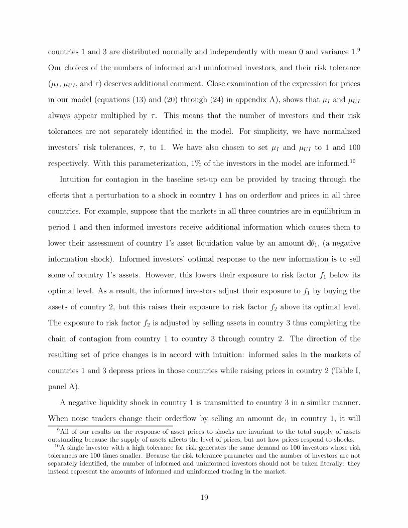
Intuition for contagion in the baseline set-up can be provided by tracing through the

effects that a perturbation to a shock in country 1 has on orderflow and prices in all three

countries. For example, suppose that the markets in all three countries are in equilibrium in

period 1 and then informed investors receive additional information which causes them to

lower their assessment of country 1’s asset liquidation value by an amount dθ1, (a negative

information shock). Informed investors’ optimal response to the new information is to sell

some of country 1’s assets. However, this lowers their exposure to risk factor f1 below its

optimal level. As a result, the informed investors adjust their exposure to f1 by buying the

assets of country 2, but this raises their exposure to risk factor f2 above its optimal level.

The exposure to risk factor f2 is adjusted by selling assets in country 3 thus completing the

chain of contagion from country 1 to country 3 through country 2. The direction of the

resulting set of price changes is in accord with intuition: informed sales in the markets of

countries 1 and 3 depress prices in those countries while raising prices in country 2 (Table I,

panel A).

A negative liquidity shock in country 1 is transmitted to country 3 in a similar manner.

When noise traders change their orderflow by selling an amount dε1 in country 1, it will

9All of our results on the response of asset prices to shocks are invariant to the total supply of assetsoutstanding because the supply of assets affects the level of prices, but not how prices respond to shocks.

10A single investor with a high tolerance for risk generates the same demand as 100 investors whose risktolerances are 100 times smaller. Because the risk tolerance parameter and the number of investors are notseparately identified, the number of informed and uninformed investors should not be taken literally: theyinstead represent the amounts of informed and uninformed trading in the market.

19

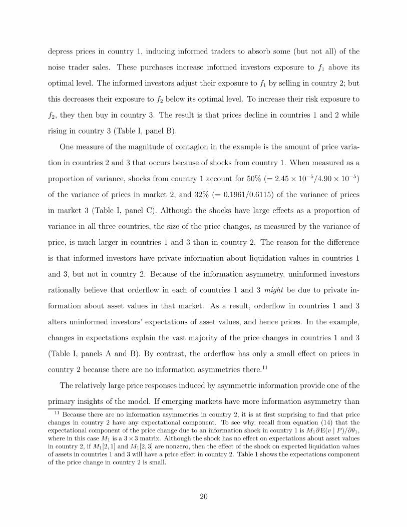
depress prices in country 1, inducing informed traders to absorb some (but not all) of the

noise trader sales. These purchases increase informed investors exposure to f1 above its

optimal level. The informed investors adjust their exposure to f1 by selling in country 2; but

this decreases their exposure to f2 below its optimal level. To increase their risk exposure to

f2, they then buy in country 3. The result is that prices decline in countries 1 and 2 while

rising in country 3 (Table I, panel B).

One measure of the magnitude of contagion in the example is the amount of price varia-

tion in countries 2 and 3 that occurs because of shocks from country 1. When measured as a

proportion of variance, shocks from country 1 account for 50% (= 2.45× 10−5/4.90× 10−5)

of the variance of prices in market 2, and 32% (= 0.1961/0.6115) of the variance of prices

in market 3 (Table I, panel C). Although the shocks have large effects as a proportion of

variance in all three countries, the size of the price changes, as measured by the variance of

price, is much larger in countries 1 and 3 than in country 2. The reason for the difference

is that informed investors have private information about liquidation values in countries 1

and 3, but not in country 2. Because of the information asymmetry, uninformed investors

rationally believe that orderflow in each of countries 1 and 3 might be due to private in-

formation about asset values in that market. As a result, orderflow in countries 1 and 3

alters uninformed investors’ expectations of asset values, and hence prices. In the example,

changes in expectations explain the vast majority of the price changes in countries 1 and 3

(Table I, panels A and B). By contrast, the orderflow has only a small effect on prices in

country 2 because there are no information asymmetries there.11

The relatively large price responses induced by asymmetric information provide one of the

primary insights of the model. If emerging markets have more information asymmetry than

11 Because there are no information asymmetries in country 2, it is at first surprising to find that pricechanges in country 2 have any expectational component. To see why, recall from equation (14) that theexpectational component of the price change due to an information shock in country 1 is M1∂ E(v | P )/∂θ1,where in this case M1 is a 3× 3 matrix. Although the shock has no effect on expectations about asset valuesin country 2, if M1[2, 1] and M1[2, 3] are nonzero, then the effect of the shock on expected liquidation valuesof assets in countries 1 and 3 will have a price effect in country 2. Table 1 shows the expectations componentof the price change in country 2 is small.

20

developed markets because public information on the value of assets in emerging markets

is less readily available, then our three-country example helps to explain the cross-sectional

differences in the pattern of contagion among emerging and developed markets.12 More

specifically, if countries 1 and 3 are viewed as emerging markets, and country 2 is viewed as

a developed market because its information asymmetries are low, then the example shows it is

possible for large price shocks to be transmitted from one set of emerging markets to another

through developed markets without significantly affecting prices in developed markets. This

may explain why emerging markets appear to have been particularly vulnerable to contagion

while developed markets have remained relatively unscathed.

When we allow a more general setting in country 2’s asset markets the pattern of con-

tagion between countries 1 and 3 is qualitatively similar, but conditions in country 2 have

interesting quantitative effects on the magnitude of price movements. In this regard, it is

important to note the role that information asymmetry in country 2 plays in the transmission

of shocks. If there is more information asymmetry in country 2, then its asset prices will be

more sensitive to orderflow. This raises the cost of rebalancing risk exposures in country 2’s

market. As a result, there will be less cross-market rebalancing from country 1 to country

2, and less rebalancing from country 2 to country 3, reducing country 3’s price response to

shocks from market 1.13 Because this example shows that more information asymmetry in

developed markets reduces contagion among emerging markets, it suggests that steps which

12 Evidence for asymmetric information in emerging markets is suggested by the results of Claessens,Djankov, and Lang (2000) who studied the ownership and control structure of publicly traded companies innine South East Asian countries. In eight of the nine countries (Japan was the exception) they found betweenone-third and one-half of market capitalization are effectively controlled by the members of 15 families.Members of such families are likely to have better information than other investors regarding a relatedcompanies’ prospects. The results of Frankel and Schmukler (1996), Froot, et. al (1998), Brennan and Cao(1997), and Seasholes (1999) also indirectly show that domestic and foreign investors may be differentiallyinformed, although the papers reach different conclusions on whether foreign or domestic investors have thebetter information.

13In equilibrium informed investors’ demands for assets in country 2 contain two components: the firstcomponent is associated with hedging factor risk, and the second is “speculative” reflecting differencesbetween market prices and the assets’ liquidation value. When there is asymmetric information in country2, informed investors’ purchases drive up prices in country 2, inducing less speculative demand for assetsin country 2. Because the speculative and hedging components are partially offsetting, the net amount ofcross-market rebalancing declines.

21

reduce information asymmetries in developed markets may have the unintended consequence

of enhancing developed markets’ role as a conduit for contagion among emerging markets.

Additionally, the importance of country-specific factors in determining liquidation values

in developed markets plays a role in determining the magnitude of contagion. When the

liquidation value of assets in country 2 is more dependent on country-specific factors, (i.e.

when the variance of η2 is larger), then more basis risk is incurred when investors use country

2 to rebalance their exposures to the common risk factors (f1 and f2). As a result, investors

incentive to rebalance across countries is reduced as are the price effects from a shock in

country 1 on prices in other countries. More noise trading in country 2 also tends to reduce

the effect that shocks in country 1 have on country 3, but for a different reason. When there

is noise trading in country 2, informed investors will take the other side and then rebalance

their positions in countries 1 and 3. Because this increases the relative likelihood that trading

in countries 1 and 3 is due to cross-market rebalancing, and not due to private information

about the asset values in countries 1 and 3, this tends to reduce the informational content

of the orderflow, and hence reduces the expectational component of the price response to

orderflow in countries 1 and 3.

The most important insight from our example is that it shows how contagion can occur

between the markets of countries 1 and 3 even when channels of contagion such as correlated

information, correlated liquidity shocks, and wealth effects are ruled out by assumption, and

even when the liquidation value of the assets in countries 1 and 3 have no macroeconomic

risk factors in common, and are in fact statistically independently distributed. This means

our model provides a possible explanation for the contagion that has been observed between

countries with different macroeconomic fundamentals. For example, our model may explain

how financial market contagion could have spread from Mexico to Asia during the Mexican

crisis in 1994, and from Asia to Latin America during the 1997-98 Asian crisis. It may also

provide insight into the transmission of market turbulence to Latin American following the

1998 Russian default.

22

Frankel and Schmukler’s (1998) study of closed-end country funds provides some support

for the transmission mechanism in our model. They showed that contagion could have spread

from Mexico through New York to Asia in the aftermath of the Mexican peso devaluation in

December 1994. Using Granger-causality tests, they examined the timing of price movements

of closed-end country funds and their net asset values (NAVs). During the Mexican crisis

they found that NAVs of Mexican funds declined before the devaluation, while the price of

Mexican closed end funds trading in New York did not decline until after the devaluation

occurred. The declines in the closed end fund prices then Granger-caused falls in funds

representing Asian stocks. Frankel and Schmukler interpreted their evidence as suggesting

that some investors were differentially informed and that, in this case, local investors in

Mexico lost confidence before investors in New York. They also found that the transmission

of shocks among emerging markets may occur indirectly through a third country.

Our main results in this section can be summarized as follows:

• Contagion can occur between countries whose long-run asset values are driven by differ-

ent macroeconomic fundamentals, provided they are linked by sharing common macroe-

conomic fundamentals with a third country or countries.

• Differences in information asymmetries between developed and emerging markets may

explain why emerging markets were hit hard by contagion while developed markets

remained relatively unscathed.

• In some circumstances, higher quality markets (in the sense of less information asym-

metry and less country-specific risk) in developed countries may worsen the contagion

among emerging markets.

In the next section we use our three-country example to examine the role of the macroe-

conomic factors in contagion.

23

IV Contagion and Fundamentals

An important focus of the policy debate on contagion centers around whether asset price

movements in those countries which are hardest hit by contagion are excessive relative to

that country’s fundamentals. In this section, we address this question in two ways. First,

we directly examine whether price movements are excessive relative to fundamentals. Then,

we contrast the role that macroeconomic fundamentals play in determining the pattern of

contagion in our model relative to more traditional models of contagion.

A Are Price Movements Excessive Relative to Fundamentals?

In the previous section we established that contagion exists between countries 1 and 3 when

contagion is defined as a shock in one country’s asset market that causes price movements

in other countries’ asset markets. In much of the literature, however, contagion is defined

more narrowly as a shock in one country that generates price movements in other countries

that are excessive relative to “full information” fundamentals. We can show that the price

movements in our three country example meets this more restrictive definition.

The analysis here relies on our earlier decomposition of the effect of shocks on asset prices

into an expectations component which measures that part of the price change that occurs

because of a change in E(v | P ), and into a portfolio balance component which measures

that part of the price change that occurs because of the reallocation of risk-sharing among

investors (equations (14) and (15)). To see how the decomposition is useful, recall that the

liquidation value of the assets in countries 1 and 3 are statistically independently distributed.

An implication of statistical independence is that conditional on full information, a shock

which all participants know originates in country 1 cannot cause a reassessment of the

expected liquidation value of the assets in country 3. Therefore any price change that occurs

because a shock in country 1 altered E(v | P ) in country 3 is excessive relative to full

information fundamentals.

24

To test for whether price movements in country 3 are excessive it suffices to examine

the expectations component of the price change in country 3 due to a shock in country 1.

In the current parameterization, the expectations component of the price changes is much

larger than the portfolio balance component (Table I, Panels A and B). The relative size

of these components is not our primary focus because it can vary for realistic values of the

number of informed and uninformed investors (see section II.A).14 The important result is

that shocks in country 1 change expectations about the value of country 3’s assets. Because

they do, price movements in country 3 due to a shock in country 1 are excessive relative to

full information fundamentals.

A more conventional method for showing that price movements are excessive relative to

full information fundamentals is to solve the model when all investors are informed and then

contrast the resulting price movements with those from the baseline model. We followed this

approach in an earlier version and reached the same conclusions.

B Role of Macroeconomic Factors in Contagion

A number of papers have explored the relationship between macroeconomic news and the

cross-sectional pattern of contagion. The general finding in this literature is that macroeco-

nomic news can account for only a small part of asset return covariation across countries at

high frequencies. Our model provides one reason for the weak explanatory power.

Recall that in the model contagion occurs in period 1, but the macroeconomic risk factors

f1 and f2 are not realized until time period 2. Moreover, before period 2 the investors receive

neither public nor private information about the factors. An immediate consequence is that

the realizations of the macroeconomic risk factors in period 2 do not influence the pattern

14In further simulations we found that for most values of µI and µUI the expectations component of theprice changes is much larger than the portfolio balance component. The exception was when the numbers ofboth types of investors were much smaller than in our baseline model, or equivalently when investors weremuch more risk averse than in our baseline model.

25

of contagion in period 1.15 This is consistent with the results that have been reported in

recent studies.16

Although the realizations of the macroeconomic risk factors do not explain the pattern

of contagion in our model, the risk factors are important, but not as used in prior models.

Instead the risk factors are central because contagion is transmitted through investors’ rebal-

ancing their portfolio’s exposures to the future risk factor realizations. Because contagion

occurs through the reoptimizing of portfolio’s risk exposures, it is the long-run macroe-

conomic risk factor structure which plays an essential role in determining the pattern of

contagion. We turn to this topic in the next section when we examine how the pattern of

contagion is influenced by assets’ sensitivities to these systematic risk factors.

V Explaining the Severity of Contagion

During each of the recent episodes of financial market contagion, the severity of the episodes

varied across countries. Our model helps to identify several characteristics which make a

country vulnerable to contagion. In this section we focus on how country 3 is affected by

two of these characteristics, the exposure of its asset values to systematic macroeconomic

risk factors, and the amount of information asymmetry within country 3. Results for how

conditions in country 3 affect other countries’ markets are available upon request.

A Role of Sensitivities to Systematic Risk Factors

In this subsection we will explore the role of an asset market’s sensitivities to the systematic

risk factors in generating contagion. Before analyzing this question in depth, it is useful

to note that Proposition 3 implies that when a country’s sensitivities (factor β’s) to the

15It is important to emphasize that our model is designed to show that it is possible to generate contagioneven in the absence of news about the macroeconomic risk factors. In a more realistic model in which newsabout the macroeconomic risk factors arrived in time period 1, it would obviously influence the pattern ofcontagion.

16See Kaminsky and Schmukler (1999), Baig and Goldfajn (1999), and Connolly and Wang (2000) asexamples.

26

common risk factors are zero, then in the cross-market rebalancing variant of our model

there is no contagion to or from that country. The intuition for this result is that when a

country’s factor β’s are zero, it shares no risk factors with other countries. Thus its markets

cannot be used for rebalancing risk factor exposures. An immediate implication is that in

the cross-market rebalancing variant of our model, contagion only occurs among countries

that are directly or indirectly linked through the sharing of common macroeconomic risk

factors.

To illustrate the role of shared risk factor exposures, we examine how country 3’s price

response to shocks in country 1 varies with β3, country 3’s exposure to risk factor f2. Be-

cause the intuition for the sign of the price response was provided in section III.B, only the

magnitude of the price response is discussed here.

The magnitude of country 3’s price response to information and liquidity shocks from

country 1 is a non-monotone function of β3. When β3 = 0, country 3 shares no risk factors

with other countries, and hence its price response is zero. As β3 increases from 0, informed

participants begin to use country 3’s market to hedge against changes in f2. This increase in

hedging activity from 0 initially increases country 3’s price response to shocks from country 1.

However, as β3 continues to grow, it becomes increasingly likely that orderflow in country 3

is due to cross-market rebalancing and not private information.17 As a result the magnitude

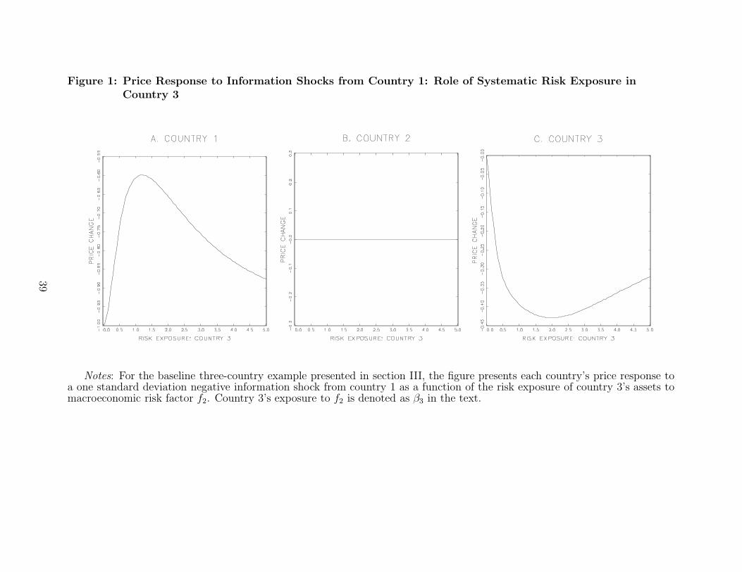
of the price response in country 3 to shocks from country 1 eventually declines (Figures 1

and 2, panel C).18

17Higher β3 reduces the relative amount of informed trading in market 3 because it increases the amountof cross-market rebalancing in country 3, and it reduces the amount of trading based on market 3’s privateinformation. This latter effect occurs because higher β3 increases the exposure to factor 2 (f2) risk thatinformed investors incur when trading on country 3’s private information.

18When the assumption of no noise traders in country 2 is relaxed then noise trading in country 2 generatesuninformative cross-market rebalancing trades in countries 1 and 3. This increase in uninformative tradingreduces the magnitude of the price response to both information and liquidity shocks emanating from country1 (not shown), but the price responses are qualitatively similar. The exception being that price responses incountry 3 to liquidity shocks from country 1 are significantly smaller and of the opposite sign as β3 rangesfrom 0 to approximately 2.5.

27

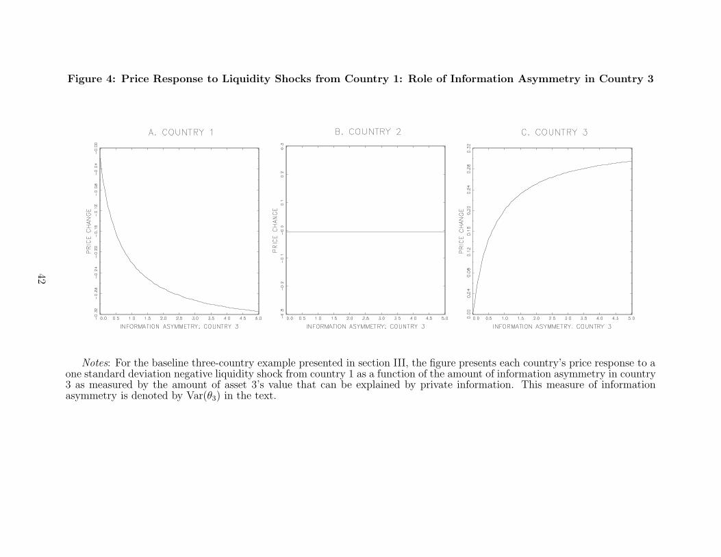
B Role of Information Asymmetry

One measure of the amount of information asymmetry in each country is the amount of

private information that informed investors have about its assets’ liquidation value. This

can be measured by the variance of θ in that country. In this subsection we examine how

price sensitivities to shocks originating in country 1 in our baseline model depend on the

amount of information asymmetry in country 3.

When there is no information asymmetry in country 3, then shocks in country 1 have

little effect on prices in country 3. As the amount of information asymmetry increases in

country 3, the price response increases monotonically. This is our most important result

because it shows that more information asymmetry in country 3 increases its vulnerability

to contagion (Figures 3 and 4, panel C). Intuition for the result is that greater information

asymmetries within a country’s market increase the likelihood that shocks transmitted to

that market from abroad will be mistakenly viewed as an information shock within that

market, magnifying price changes.

C Summary

Our principal results on the role of risk factor sensitivities and information asymmetries are

restated below:

• Contagion occurs across countries whose asset values are linked through sharing expo-

sures (β) to common macroeconomic fundamentals. Increases in β from zero increase

a country’s vulnerability to contagion.

• When β is not equal to zero, changes in β do not have a simple relationship to the

pattern of contagion and can either increase or decrease a country’s vulnerability to

shocks from abroad.

• More information asymmetry within a country’s asset market increases the magnitude

of that market’s price response to contagion from abroad.

28

VI Explaining the Pattern of Contagion Across Coun-

tries and Through Time

One shortcoming of the model is that it is static, and the parameters of the model are

fixed. As a result, the model helps to explain the cross-country pattern of financial market

contagion, but makes no predictions about how it changes through time. In particular,

the model, considered alone, cannot explain why financial market contagion appears to be

more acute during some time periods than others. One way to gain further insight into the

dynamics of contagion is to treat the model’s parameters as being formally determined by

other elements of the economic environment. In particular, we consider how changes in some

of these elements affect two determinants of a country’s vulnerabilty to financial contagion:

the sensitivity of a country’s asset values to fluctuations in systematic macroeconomic factors,

and the amount of information asymmetry within a country.

One important element that could cause time variation in the sensitivity of an asset mar-

ket to the risk factors is a country’s movement from a fixed to flexible exchange rate regime.

A regime switch of this sort adds an important risk by increasing a country’s asset market

exposure to exchange rate fluctuations from zero, opening up the potential for contagion

through cross-market rebalancing. An alternative explanation for time variation in risk fac-

tor sensitivities is the dramatic increase in financial leverage experienced by some companies

during an exchange rate or financial crisis. For example, during the Asian financial crisis, ex-

change rate devaluations in some countries dramatically increased the market value of many

companies’ foreign-denominated debt obligations and dramatically reduced the market value

of shareholders’ equity, raising their debt-equity ratios. The increase in financial leverage

increases factor sensitivities and can substantially alter the pattern of contagion.

Changes in informational asymmetries, as a result of the onset of banking and financial

crises in some countries, may also help explain the time-series pattern of contagion in the

context of our model. Although there are many ways asymmetric information could manifest

29

itself, one type of informational advantage that some investors could have is superior knowl-

edge of various companies’ financial condition, and those companies’ access to emergency

sources of credit. It could also represent some investors’ differential access to knowledge

about government economic policy. For instance, Claessens, Djankov, and Lang (2000) note

that the families which control large chunks of market capitalization in the countries in South

East Asia often have close ties to government. When macroeconomic conditions are stable

most companies will be in sound financial condition, and therefore knowledge of companies’

access to emergency funding from public or private sources will have relatively little value.

Therefore, in good times the degree of information asymmetry will be low. During financial

or banking crises, the same type of information becomes very valuable in establishing prices

for companies’ equity. Consequently informational asymmetries, as measured by the value

of what the better informed investors know, become larger. More generally, during financial

and banking crises, anecdotal evidence suggests a great deal of confusion about the values

of companies, lending credence to an increase in informational asymmetries during these

periods.

The recent abrupt changes in exchange rate regimes from fixed to floating, and the

increases in financial leverage experienced by many corporations in emerging markets during

financial crises, increase parameters in our model which are linked to increased vulnerability

to financial market contagion. We believe this provides some additional insight into why

financial market contagion has increased recently, and how the pattern of financial market

contagion might change through time.

VII Conclusions

In this paper we presented a multiple asset, noisy rational expectations model of asset prices

and used the model to study the determinants of financial market contagion over short pe-

riods of time such as a day or a week. The model nests the correlated information and

correlated liquidity shock channels for contagion considered by others and also contains a

30

new channel which we refer to as cross-market rebalancing. Contagion occurs through this

third channel when market participants are hit with an idiosyncratic shock in one coun-

try and transmit the shock abroad by optimally rebalancing their portfolio’s exposures to

macroeconomic risks through other countries’ markets. Countries whose asset values are

driven by common macroeconomic factors are vulnerable to this form of contagion, but it

can also occur between two countries whose asset values are determined by independent

macroeconomic factors, provided they are indirectly linked through third countries. Cross-

market rebalancing may thus explain contagion between Asia and Latin America during

recent crises even though the macroeconomies of the two regions are only weakly linked.

One of our most important findings is that asymmetric information makes a country more

vulnerable to contagion from abroad. Most of the contagious price response in a given country

occurs because the order flow from cross-market rebalancing from other countries is partially

misinterpreted as being related to information about asset values within that particular

country. The model suggests that one possible protection against undesired, excessive price

movements is a reduction in informational asymmetries through better transparency and

more open access to information underlying the value of assets. The model also shows

the rather perverse result that as informational asymmetries shrink in developed countries’

markets, these countries act to transmit contagion among emerging market countries rather

than contain it.

To close, it is useful to relate our paper to the contagion literature which stresses macroe-

conomic channels. Our theoretical model and this literature both are built upon the common

notion that macroeconomic fundamentals are an important element of contagion, but we use

these fundamental relations in a new way. Instead of looking to the realizations of macroe-

conomic fundamentals or macroeconomic news to rationalize the pattern of financial market

contagion (an approach which appears to explain little empirically), we model long-run asset

values across countries as depending on common macroeconomic factors and we model con-

tagion as a consequence of the optimal rebalancing of exposures to macroeconomic risks. In

31

this framework, contagion does not depend on macroeconomic news. Nor do macroeconomic

fundamentals need to be realized for contagion to occur. Portfolio rebalancing within this

framework, however, would be relatively benign if it were not for the presence of asymmetric

information. Information asymmetries help to account for why asset price movements are

far larger in some countries than can be justified by the movements of their macroeconomic

fundamentals. One can also use the model to consider how some of the parameters change

through time, providing additional insight into the timing of contagious episodes. Thus,

by combining portfolio rebalancing and information asymmetries, our model identifies an

additional channel for contagion that can formally explain why some countries are hit, and

hit hard, by contagious episodes while others are not.

32

Appendix

A Equilibrium Beliefs, Prices, and the Variance of Prices

In this section of the appendix we solve for equilibrium beliefs for the general model de-

scribed in section I. The equilibrium beliefs are solved for by imposing the belief consistency

conditions in equations (11) and (12) while exploiting the normality of S(P ), θ, and ε. Using

the right hand side of the expression for S(P ) (equation (9)) and the joint distribution of θ

and u (equation (2)), the equilibrium beliefs are:

E(v | P ) = E(v | S(P ))

= v + Cov[S(P ), v][Var(S(P ))]−1[S(P )− E{S(P )}]

= θ + Σθ

[Σθ +

ΣuΣεΣu

(τµI)2

]−1

[S(P )− θ]

= θ + Σθ

[Σθ +

ΣuΣεΣu

(τµI)2

]−1 [θ +

Σuε

τµI− θ

], (18)

and

Var(v | P ) = Var(v | S(P ))

= Σv − Cov(v, S(P ))[Var(S(P ))]−1Cov(v, S(P ))′

= [Σθ + Σu]− Σθ

[Σθ +

ΣuΣεΣu

(τµI)2

]−1

Σθ′. (19)

Equations (18) and (19) are not explicit functions of equilibrium price, but are instead

consistency conditions on beliefs that must be satisfied by the equilibrium price function.19

Equilibrium prices are found by rewriting the market clearing condition (equation (8)) to

solve for price P as a function of the expressions for E(v | P ) and Var(v | P ) from equa-

19It is possible to solve for E(v | P ) as an explicit function of P . The solution is:

E(v | P ) = φ0 + φ1v + φ2P

33

tions (18) and (19). Repeating from proposition 1, the rational expectations equilibrium

price function P for the model described by equations (1), (2),(4),(6), and (7) is

P = M0 + M1 E(v | P ) + M2 θ + M3 ε

where,

M0 = −Ψ−1XT (20)

M1 = Ψ−1µUIτ [Var(v | P )]−1 (21)

M2 = Ψ−1µIτΣ−1u (22)

M3 = Ψ−1 (23)

Ψ = µUIτ [Var(v | P )]−1 + µIτΣ−1u , (24)

and E(v | P ) and Var(v | P ) are given in equations (18) and (19).

Based on the expression for price, it follows that the unconditional variance of P is:

Var(P ) = Ψ−1(CΣθC′ + DΣεD

′)Ψ−1, (25)

where:

φ =[I + Cov(S(P ), v)[Var(S(P ))]−1 (1 − µI)

µIΣu Var(v | P )−1

]

φ0 = φ−1

(Cov(S(P ), v)[Var(S(P ))]−1 Σu

(τµI)[XT

])

φ1 = φ−1(I − Cov(S(P ), v)[Var(S(P ))]−1

)

φ2 = φ−1

(Cov(S(P ), v)[Var(S(P ))]−1 Σu

τµI

[µUIτ [Var(v | P )]−1 + τµIΣ−1

u )])

Var(v | P ) cannot be written as a function of price because prices reveal no information on the variance of vbeyond that which is contained in knowledge of the structure of the model.

34

where

C = µUIτ [Var(v | P )]−1Σθ

[Σθ +

ΣuΣεΣu

(τµI)2

]−1

+ µIτΣ−1u

D =CΣu

µIτ

B Proof of Propositions 2 and 3

Proposition 2. If Σθ, Σu, and Σε are all diagonal matrices, then there is no contagion from

any market to any other market.

Proof: Under the conditions of the proposition, inspection shows the derivatives of E(v | P )

(equation (18)) with respect to ε and θ are diagonal matrices, as are Var(v | P ) (equation

(19)), Ψ (equation (24)), and Σu. Their sums, products, and inverses are also diagonal.

Therefore, evaluating equations (14) and (15) while using the expressions for M1, M2, and

M3 from equations (21), (22), and (23) shows that ∂P/∂ε and ∂P/∂θ are both diagonal

matrices. Hence, there is no contagion.

Proposition 3. If one of the matrices Σθ, Σu, or Σε is block diagonal, and the other two

matrices are conformably block diagonal with it, then there is contagion between the markets

within a particular block but no contagion between markets in different blocks.

Proof: If for some common partition, the matrices Σθ, Σu, and Σε are conformably block

diagonal, then their sums, products, and inverses are all conformably block diagonal with the

same partition of the elements of the matrices. Because ∂P/∂θ and ∂P/∂ε involve only the

sums products and inverses of these matrices, it then follows that ∂P/∂θ, and ∂P/∂ε are

block diagonal for the same common partition. Therefore, it follows that there is no conta-

gion between assets (or markets) in different blocks.

35

BIBLIOGRAPHY

Admati, Anat R., 1985, A noisy rational expectations equilibrium for multi-asset securitiesmarkets, Econometrica 53, 629-657.

Agenor, Pierre-Richard, and Joshua Aizenman, 1998, Contagion and volatility with imper-fect credit markets, IMF Staff Papers 45, 207-235.

Allen, Franklin, and Douglas Gale, 2000, Financial contagion, Journal of Political Economy108, 1-33.

Baig, Taimur, and Ilan Goldfajn, 1999, Financial markets contagion in the asian crises,IMF Staff Papers 46, 167-195.

Brennan, Michael J., and H. Henry Cao, 1997, International portfolio investment flows,Journal of Finance 52, 1851-1880.

Caballero, Ricardo, and Arvind Krishnamurthy, 1999, Emerging market crises: an assetmarkets perspective, IMF Working Paper No. 99/129, (International Monetary Fund,Washington, DC).

Calvo, Guillermo A., 1999, Contagion in emerging markets: when Wall Street is a carrier,Working paper, University of Maryland.

Chan-Lau, Jorge A., and Zhaohui Chen, 1998, Financial crisis and credit crunch as a resultof inefficient financial intermediation—with reference to the asian financial crisis, IMFWorking Paper No. 98/127, (International Monetary Fund, Washington DC).

Claessens, Stijn, Simeon Djankov, and Larry H.P. Lang, 2000, Separation of ownership andcontrol in east asian countries, Journal of Financial Economics 158, 81-112.

Connolly, Robert A., and F. Albert Wang, 2000, On stock market return comovements:macroeconomic news, dispersion of beliefs, and contagion, Working paper, Universityof North Carolina and Rice University.

Corsetti, Giancarlo, Paolo Pesenti, and Nouriel Roubini, 1999, Paper tigers? A model ofthe asian crisis, European Economic Review 43, 1211-1236.

Fleming, Jeff, Chris Kirby, and Barbara Ostdiek, 1998, Information and volatility linkagesin the stock, bond, and money markets, Journal of Financial Economics 49, 111-137.

Frankel, Jeffrey A., and Sergio L. Schmukler, 1998, Crises, contagion, and country funds: ef-fects on east asia and latin america, in Reuven Glick, ed.: Managing Capital Flows andExchange Rates: Perspectives from the Pacific Basin, (Cambridge University Press,Cambridge).

Frankel, Jeffrey A., and Sergio L. Schmukler, 1996, Country fund discounts and the mex-ican crisis of December 1994: did local residents turn pessimistic before internationalinvestors? Open Economies Review(Suppl. 1) 7, 551-34.

Froot, Kenneth A., Paul G.J. O’Connell, and Mark S. Seasholes, 1998, The portfolio flowsof international investors: I, NBER Working Paper No. 6687, (Boston, MA).

Gennotte, Gerard, and Hayne Leland, 1990, Market liquidity, hedging, and crashes, Amer-ican Economic Review 80, 999-1021.

36

Goldfajn, Ilan, and Rodrigo O. Valdes, 1997, Capital flows and the twin crises: The role ofliquidity, IMF Working Paper No. 97/87, (International Monetary Fund, WashingtonDC).

Grossman, Sanford J., and Joseph E. Stiglitz, 1980, On the impossibility of informationallyefficient markets, American Economic Review 70, 393-408.

Kaminsky, Graciela L., and Carmen M. Reinhart, 2000, On crises, contagion, and confusion,Journal of International Economics 51, 145-168.

Kaminisky, Graciela L., and Serio L. Schmukler, 1999, What triggers market jitters? Achronicle of the asian crisis, Journal of International Money and Finance 18, 537-560.

King, Mervyn A., and Sushil Wadhwani, 1990, Transmission of volatility between stockmarkets, Review of Financial Studies 3, 5-33.

Kyle, Albert S., and Wei Xiong, 2001, Contagion as a wealth effect, Forthcoming Journalof Finance, Papers and Proceedings.

Lagunoff, Roger D., and Stacey L. Schreft, 2001, A model of financial fragility, ForthcomingJournal of Economic Theory.

Pritsker, Matt G., 1997, Liquidity risk and positive feedback, in The Measurement of Ag-gregate Market Risk (Bank for International Settlements, Basle).

Rigobon, Roberto, 1998, Informational speculative attacks: good news is no news, Workingpaper, Massachusetts Institute of Technology.

Schinasi, Garry J., and R. Todd Smith, 2000, Portfolio diversification, leverage, and finan-cial contagion, IMF Staff Papers 47, 159-176.

Seasholes, Mark S., 1999, Smart foreign traders in emerging markets, Working paper, Har-vard University Business School.

Van Rijckeghem, Caroline, and Beatrice Weder, 2000, Spillovers through banking centers:a panel data analysis, IMF Working Paper No. 00/88, (International Monetary Fund,Washington, DC).

Wang, Jiang, 1993, A model of intertemporal asset prices under asymmetric information,Review of Economic Studies 60, 249-282.

Wang, Jiang, 1994, A model of competitive stock trading volume, Journal of PoliticalEconomy 102, 127-168.

Yuan, Kathy, 2000, Asymmetric price movements and borrowing constraints: a rationalexpectations equilibrium model of crisis, contagion, and confusion, Ph.D. Dissertation,Massachesetts Institute of Technology.

Zhou, Chunsheng, 1998, Dynamic portfolio choice and asset pricing with differential infor-mation, Journal of Economic Dynamics and Control 22, 1027-51.

37

Table I: Price Response to Shocks from Market 1: Baseline Case

A. Negative Information Shock

Market 1 Market 2 Market 3Expectations Component -0.5937 1.67× 10−17 -0.3964Portfolio Balance Component -0.0119 3.04× 10−18 0.0020

Total -0.6055 1.97× 10−17 -0.3945

B. Negative Liquidity Shock

Market 1 Market 2 Market 3Expectations Component -0.1972 5.55× 10−18 0.1972Portfolio Balance Component -0.0237 -0.0050 0.0039

Total -0.2209 -0.0050 0.2011

C. Variance of Prices

Market 1 Market 2 Market 3From Market 1 Shocks 0.4155 2.4507× 10−5 0.1961From Market 3 Shocks 0.1961 2.4507× 10−5 0.4155

Total 0.6115 4.90× 10−5 0.6115

Notes: For the baseline three-country example presented in section III, the price of riskyassets in all three countries are a linear function of the liquidity and information shocksthat originate in country 1. The linear sensitivities of prices to the shocks are presentedin panels A and B. The price sensitivities are further decomposed into an expectations andportfolio balance component. The expectations component measures that part of the pricesensitivity that is due to shocks causing revisions in investors’ beliefs. The portfolio balancecomponent measures that part of the price sensitivity which occurs because shocks lead tothe reallocation of risky asset holdings among market participants. Panel C decomposes thevariance of prices in each market into the variance which is due to shocks from market 1 andthe variance which is due to shocks from market 3.

38

Figure 1: Price Response to Information Shocks from Country 1: Role of Systematic Risk Exposure inCountry 3

Notes: For the baseline three-country example presented in section III, the figure presents each country’s price response toa one standard deviation negative information shock from country 1 as a function of the risk exposure of country 3’s assets tomacroeconomic risk factor f2. Country 3’s exposure to f2 is denoted as β3 in the text.

39

Figure 2: Price Response to Liquidity Shocks from Country 1: Role of Systematic Risk Exposure in Country 3

Notes: For the baseline three-country example presented in section III, the figure presents each country’s price response toa one standard deviation negative liquidity shock from country 1 as a function of the risk exposure of country 3’s assets tomacroeconomic risk factor f2. Country 3’s exposure to f2 is denoted as β3 in the text.

40

Figure 3: Price Response to Information Shocks from Country 1: Role of Information Asymmetry inCountry 3

Notes: For the baseline three-country example presented in section III, the figure presents each country’s price response toa one standard deviation negative information shock from country 1 as a function of the amount of information asymmetryin country 3 as measured by the amount of asset 3’s value that can be explained by private information. This measure ofinformation asymmetry is denoted by Var(θ3) in the text.

41

Figure 4: Price Response to Liquidity Shocks from Country 1: Role of Information Asymmetry in Country 3

Notes: For the baseline three-country example presented in section III, the figure presents each country’s price response to aone standard deviation negative liquidity shock from country 1 as a function of the amount of information asymmetry in country3 as measured by the amount of asset 3’s value that can be explained by private information. This measure of informationasymmetry is denoted by Var(θ3) in the text.

42