A Rational Theory for Disposition Effects * Min Dai Yipeng Jiang Hong Liu Jing Xu May 23, 2021 * We are grateful to Vincenzo Quadrini (the editor), an anonymous referee, Georgy Chabakauri (EFA discussant), Bing Han, David Hirshleifer, Philipp Illeditsch (SFS Cavalcade discussant), Stijn Van Nieuwerburgh, Kenneth Singleton, Dimitri Vayanos, Liyan Yang, and seminar participants at Aus- tralian National University, the 28 th AFB Conference, Boston University, CKGSB, 2016 EFA Annual Meeting, National University of Singapore, 2016 SFS Cavalcade, 2016 SIF conference, Singapore Man- agement University, Tsinghua University, University of Calgary, University of Melbourne, University of New South Wales, University of Rochester, Universite Paris Diderot, Renmin University of China, and Washington University in St. Louis for helpful comments. We thank Terrance Odean for providing us with the brokerage trading data used in Odean (1998). This paper was previously circulated under the title “Multiple Birds, One Stone: Can Portfolio Rebalancing Contribute to Disposition-effect-related Trading Patterns?” Min Dai and Yipeng Jiang are from National University of Singapore, Hong Liu is from Washington University in St. Louis and CHIEF, and Jing Xu is from Renmin University of China. Authors can be reached at [email protected], [email protected], [email protected], and [email protected], respectively. The authors have no conflicts of interests to disclose.
Transcript
A Rational Theory for Disposition Effects ∗
Min Dai Yipeng Jiang Hong Liu Jing Xu
May 23, 2021
∗We are grateful to Vincenzo Quadrini (the editor), an anonymous referee, Georgy Chabakauri(EFA discussant), Bing Han, David Hirshleifer, Philipp Illeditsch (SFS Cavalcade discussant), StijnVan Nieuwerburgh, Kenneth Singleton, Dimitri Vayanos, Liyan Yang, and seminar participants at Aus-tralian National University, the 28th AFB Conference, Boston University, CKGSB, 2016 EFA AnnualMeeting, National University of Singapore, 2016 SFS Cavalcade, 2016 SIF conference, Singapore Man-agement University, Tsinghua University, University of Calgary, University of Melbourne, University ofNew South Wales, University of Rochester, Universite Paris Diderot, Renmin University of China, andWashington University in St. Louis for helpful comments. We thank Terrance Odean for providing uswith the brokerage trading data used in Odean (1998). This paper was previously circulated under thetitle “Multiple Birds, One Stone: Can Portfolio Rebalancing Contribute to Disposition-effect-relatedTrading Patterns?” Min Dai and Yipeng Jiang are from National University of Singapore, Hong Liuis from Washington University in St. Louis and CHIEF, and Jing Xu is from Renmin University ofChina. Authors can be reached at [email protected], [email protected], [email protected], [email protected], respectively. The authors have no conflicts of interests to disclose.
A Rational Theory for Disposition Effects
Abstract
Extant theories on the disposition effect are largely silent on most of the disposition-
effect related trading patterns, including the V-shaped probabilities of buying and selling
against unrealized profit. On the other hand, portfolio rebalancing and learning have been
shown to be important, even for retail investors. We show that rational rebalancing with
transaction costs and unknown expected returns can generate many disposition-effect-
related trading patterns, including the V-shape results. Our paper complements the
extant theories by suggesting that portfolio rebalancing may also constitute a significant
driving force behind the disposition effect and the related patterns.
Journal of Economic Literature Classification Numbers: G11, H24, K34, D91.
The disposition effect, which is the tendency of investors to sell winners while holding
onto losers, has been widely documented in the empirical literature. For example, using
data containing 10,000 stock investment accounts in a U.S. discount brokerage from 1987
to 1993, Odean conducts a set of tests of the disposition effect hypothesis in his seminal
work of Odean (1998). He concludes that the disposition effect exists across years and
investors.1 Closely related to the disposition effect, Ben-David and Hirshleifer (2012)
show that the plots of the probabilities of selling and of buying more of some existing
shares against unrealized profit both exhibit V-shape patterns, i.e., as the magnitudes
of unrealized profits/losses increase, these probabilities also increase. Theories based on
prospect theory, mental accounting, regret aversion, and gain/loss realization utility to
explain the disposition effect have dominated the literature.2 However, it is difficult for
extant theories to explain the V-shape patterns. In addition, as far as we know, there
have been no theoretical models proposed to explain other well-documented disposition
effect-related patterns, such as: 1) investors may sell winners that subsequently outper-
form losers that they hold (Odean (1998)); 2) the disposition effect is stronger for less
sophisticated investors (Dhar and Zhu (2006)); 3) the disposition effect may increase
with return volatility (Kumar (2009)); and 4) investors are reluctant to repurchase stocks
previously sold for a loss, as well as stocks that have appreciated in price subsequent to
a prior sale (Strahilevitz, Odean, and Barber (2011)).
Another strand of literature documents that portfolio rebalancing is an important
1 See also, Shefrin and Statman (1985), Grinblatt and Keloharju (2001), Kumar (2009), Ivkovic andWeisbenner (2009), and Engelberg, Henriksson, and Williams (2018).
2 See, for example, Shefrin and Statman (1985), Odean (1998), Barberis and Xiong (2009), Ingersolland Jin (2013), Chang, Solomon, and Westerfield (2016), and Frydman, Hartzmark, and Solomon (2018).While these theories do seem to offer a promising framework for understanding the disposition effect,the possible link has almost always been discussed in informal terms, with one notable exception. Usinga rigorous model, Barberis and Xiong (2009) demonstrate that assuming prospect theory utility onrealized gains/losses can potentially predict a disposition effect. However, by examining a realizationutility model with adaptive reference points, He and Yang (2019) cast doubt on whether realizationutility is the driving force behind the disposition effect. Moreover, from a behavioral perspective, it canbe puzzling that even the professional traders still display the disposition effect at no economic cost (e.g.Frino, Johnstone, and Zheng (2004)), as these traders are believed to be less prone to behavioral bias.
2
driver behind even retail investors’ trading.3 For example, Calvet, Campbell, and Sodini
(2009) find strong household-level evidence of active rebalancing by retail investors who
typically hold a small number of stocks. Using a sample of Japanese retail investors
from 2013 to 2016, Komai, Koyano, and Miyakawa (2018) find that investors tend to
conduct contrarian trades, as predicted by standard portfolio rebalancing models. In
addition, trading patterns consistent with rational learning by investors have been widely
documented. For example, Grinblatt and Keloharju (2001) report that past returns
and historical price patterns affect trading decisions in ways that are consistent with
rational learning. Kandel, Ofer, and Sarig (1993) and Banerjee (2011) provide evidence
that investors learn about information contained in asset prices and revise their trading
strategy accordingly. Furthermore, even though transaction costs have declined in recent
years, bid-ask spreads and other trading costs (e.g., brokerage fees and time costs) remain
significant, especially for retail investors. As a result, investors do not trade continuously
(e.g., Davis and Norman (1990), Liu (2004)).
As extant literature has shown (e.g., Odean (1998)), portfolio rebalancing without any
market friction cannot explain the disposition effect. Based on the aforementioned empir-
ical evidence on the importance of portfolio rebalancing, learning, and transaction costs,
we develop an optimal portfolio rebalancing model with transaction costs and incomplete
information (in the form of unknown expected returns) to examine whether rational port-
folio rebalancing in the presence of these frictions can help explain the disposition effect
and related trading patterns of retail investors. We show that, indeed, in the presence
of these frictions, portfolio rebalancing can lead to the disposition effect and many of
the related patterns, including the V-shape patterns. While we believe that behavioral
types of explanations are essential in understanding the disposition effect and the related
trading patterns, our finding suggests that portfolio rebalancing may also constitute a
significant driving force behind these results and thus complement the extant theories.
More specifically, we consider a portfolio rebalancing model in which a small retail
3 In our analysis, we refer to trading of individual stocks to achieve the optimal portfolio determinedby the risk-return tradeoff as portfolio rebalancing.
3
investor (i.e., one who has no price impact) can trade a risk-free asset and multiple risky
assets (“stocks”) to maximize the expected utility from the final wealth at a finite hori-
zon.4 The stocks’ expected returns are unknown and the investor updates the conditional
distributions of the expected returns after observing past returns. Trading the stocks is
subject to proportional transaction costs.
To make our expositions as clear as possible, we consider two sets of model parameters.
We begin with a case where stocks have homogeneous return-risk profiles and uncorrelated
returns. This is a clean setting to illustrate the main working mechanisms. Then, we
show that these mechanisms continue to work with calibrated parameter values with
heterogeneous risk-return profiles and correlated returns.
We show that the optimal rebalancing strategy implied by our model can exhibit a
disposition effect. For example, for a reasonable set of parameter values, the ratio of the
number of realized gains to the number of all gains (realized gains plus paper gains), i.e.,
PGR, is 0.331, while the ratio of the number of realized losses to the number of all losses
(realized losses plus paper losses), i.e., PLR, is 0.168. These results indicate that the
investor exhibits greater propensity of realizing gains than losses.
The main driving force for the disposition effect displayed in our model is the “ex-
posure effect.” Intuitively, for a risk-averse utility maximizing investor, it is optimal to
keep the exposure to a stock within an upper bound and a lower bound to trade off risks
and returns. A rise in the price of a stock results in a gain and increases the investor’s
risk exposure to this stock. If the exposure increases above the upper bound, then it
is optimal to sell and thus realize a gain. A fall in the stock price results in a loss and
decreases the investor’s risk exposure. If the exposure decreases below the lower bound,
then it is optimal to buy, not sell, additional shares. It is this asymmetry (i.e., selling
with a large gain, but buying with a large loss) due to the exposure effect that makes
investors realize gains more often than losses. On the other hand, if the exposure after
4 As in the existing literature on the disposition effect (e.g., Shefrin and Statman (1985), Barberisand Xiong (2009), and Ingersoll and Jin (2013)), we use a partial equilibrium setting because most ofthe empirical studies on the disposition effect and the related trading patterns focus on retail investors,whose trading unlikely affects market prices.
4
a gain or loss is still within the bounds, the investor does not trade, due to the presence
of transaction costs. Because selling a stock with a loss requires the upper bound of
the risk exposure to be reached after a decline in the stock price and buying additional
shares after a loss requires the lower bound to be reached, investors hold onto losers after
small losses. Thus, the combination of the exposure effect and the presence of transaction
costs makes investors tend to sell winners and hold onto losers, consistent with existing
empirical findings. Because the exposure effect exists for any risk-averse utility maximiz-
ing investors, the above qualitative results apply to all risk-averse preferences, such as
CRRA, CARA, and Epstein-Zin preferences.5
It is empirically found that past returns also significantly affect investors’ trading
behavior. Using a data set containing all common stock trades of Finnish household
investors from 1995 to 2000, Kaustia (2010) provides the first evidence that the investors’
selling propensities increase in the magnitude of gains. Ben-David and Hirshleifer (2012)
further demonstrate that the probability of buying more and of selling are both greater
for positions with larger paper gains or larger paper losses.6 Theories based on the static
prospect theory, or regret aversion, predict that the larger the loss, the less likely it is for
investors to sell, and the larger the gain, the less likely it is for investors to buy, which
is opposite of the V-shape pattern. Ben-David and Hirshleifer (2012) argue that the V-
shape pattern can be consistent with change of perceptions and faiths (belief revision).
Assuming that an investor can obtain a burst of reference-dependent utility from a sale
in a dynamic prospect theory setting, Ingersoll and Jin (2013) demonstrate that the
probability of selling can increase with the magnitude of losses because there is a benefit
of realizing losses to reset references in this dynamic setting.7 Peng (2017) attributes the
5 For example, for CARA preferences, it is optimal to keep the dollar amount in a stock in a range,and for CRRA preferences and some Epstein-Zin preferences, it is optimal to keep the fraction of wealthin a stock in a range as in our model. For all of these preferences, it is optimal to sell when the stockprice rises sufficiently, and to buy when the stock price decreases sufficiently.
6 Note that the evidence that the probability of selling increases with loss magnitudes is not contra-dictory to the disposition effect, because the unconditional probability of selling losers is still smallerthan that of selling winners. An (2016) and An and Argyle (2016) find that stocks with both largeunrealized gains and large unrealized losses outperform others in the following month. This finding maybe consistent with V-shape trading patterns.
7 For a discussion of realization utility theory, see also Barberis and Xiong (2012).
5
V-shaped selling pattern to irrational extrapolation of past returns.
We show that the V-shape patterns for both the purchase probability and the sale
probability are consistent with the optimal trading strategy in our portfolio rebalancing
model. Intuitively, two opposing forces exist in our model: the “exposure effect” and the
“learning effect.” As previously explained, the exposure effect tends to make investors sell
after a large gain but buy after a large loss (“buy low, sell high”), exhibiting a contrarian
trading strategy. In contrast, the learning effect tends to make investors buy after a large
gain and sell after a large loss (“buy high, sell low”), exhibiting a momentum trading
strategy. This is because investors revise upward their estimate of expected returns after
gains and do the opposite after losses. The patterns of the probability of selling increasing
with the magnitude of gains and the probability of buying increasing with the magnitude
of losses are driven by the exposure effect. On the other hand, because there is a greater
increase (decrease) in the estimate of the expected return after observing a large gain
(loss), the probability of buying more (selling) is greater for a large gain (loss) than for a
small gain (loss).8 Thus, the patterns of the probability of buying more increasing with
the magnitude of gains and the probability of selling increasing with the magnitude of
losses are driven by the learning effect. The relative strength of the two effects determines
the trading direction. In our model, it is the coexistence of the exposure effect and the
learning effect that drives the V-shape patterns.
Moreover, in contrast to the existing literature, our model can generate many other
disposition effect-related patterns documented in empirical studies, such as those four
stated at the end of the first paragraph. As in the previous results, the driving forces
behind these results are also the presence of, and the interaction between, the exposure
effect and the learning effect. For example, less sophisticated investors may have less
learning capability than more sophisticated investors. As a result, the learning effect
may be smaller and the disposition effect may be stronger for less sophisticated investors.
For ease of reference, we summarize the main results and driving mechanisms in Table
8 The conditional volatility of the expected return deterministically decreases over time. Its impactis largely dominated by the impact of the change in the estimate of the expected return, especially whenthere are large return shocks. See Section 3 for more detailed discussions.
6
Table 1: Main results and driving mechanisms
This table summarizes the main patterns predicted by our model and the driving mechanisms.
Repurchase patternsFor winners/lossers at the time of sales Learning effectFor winners/lossers since last sale Exposure effect
Table 2: Comparison with existing papers
This table reports a comparison between the trading patterns examined in our paper and inbehavioral models in the literature.
DE RDE Volatility pattern V-shape Repurchase
Barberis and Xiong (2009) Yes No No No NoIngersoll and Jin (2013) Yes No No Yes NoPeng (2017) Yes No No Yes NoThis paper Yes Yes Yes Yes Yes
1, and a comparison between our paper and some existing papers in Table 2.
It is well known that, with capital gains tax, realizing losses sooner and deferring
capital gains can provide significant benefits (e.g., Constantinides (1983)). This force
acts against the disposition effect. We demonstrate that, consistent with the empirical
findings of Lakonishok and Smidt (1986), the disposition effect can still arise in an optimal
portfolio rebalancing model with capital gains tax and transaction costs. Intuitively,
when a stock’s price appreciates sufficiently, the investor’s risk exposure to this stock can
become too high, and the benefit of lowering the exposure by a sale can dominate the
benefit of deferring the realization of gains. In addition, with transaction costs, realizing
losses immediately is no longer optimal, and deferring even large capital losses may be
7
optimal. This is because the extra time value obtained from realizing losses sooner can
be outweighed by the transaction cost payment, even when the transaction cost is small.
Our model offers some new empirically testable predictions for future studies. For
example, our model predicts that: (1) conditional on return volatility, the magnitude
of the disposition effect is greater for stocks for which there is more public information,
because for these stocks much is already known, and thus the learning effect is smaller;
(2) investors with a more diversified portfolio or a better hedged portfolio have a weaker
disposition effect, because for these portfolios the exposure effect is smaller; and (3) the
V-shaped trading patterns are more pronounced for stocks with less public information,
because the learning effect is stronger for these stocks.
Although we consider a small investor whose trades have no price impact and thus
adopt a partial equilibrium approach, the disposition effect can arise in equilibrium (e.g.,
Basak (2005), Dorn and Strobl (2009)). For example, Dorn and Strobl (2009) demon-
strate that, in the presence of information asymmetry, the less informed become con-
trarians while the more informed become momentum traders in equilibrium. The less
informed investors in their model trade in the same way as the investor in our model, and
thus displays the disposition effect in equilibrium. The fact that in equilibrium for each
investor who sells there must be a counterparty who buys does not imply that there is no
disposition effect on average. This is because it is possible that a greater number of retail
investors with a stronger disposition effect trade with a small number of institutional
investors, for example, and most of the studies of the disposition effect and the related
trading patterns focus on retail investors.
The remainder of the paper proceeds as follows. In the next section, we present the
main model and theoretical analysis. In Section 3, we numerically solve the model and
conduct simulations to illustrate that our model can generate most of the disposition-
effect related patterns. We also show that the disposition effect can exist even with capital
gains tax. We conclude with Section 4, and all proofs are provided in the Appendix.
8
2 The Model
In this section, we describe the main ingredients of our model. We extend the model of
Cvitanic, Lazrak, Martellini, and Zapatero (2006) to incorporate transaction costs. As
we have discussed in the Introduction, the inclusion of transaction costs is necessary to
generate some disposition effect-related patterns. Moreover, incorporating transaction
costs in a multi-stock model is a highly challenging task.
2.1 Economic setting
We consider the optimal investment problem of a small retail investor (i.e., a price taker)
who maximizes the expected constant relative risk-averse (CRRA) utility from the final
wealth at some finite time T > 0.9 The investor can invest in one risk-free asset (“bond”)
and N ≥ 1 risky assets (“stocks”). The bond offers a constant interest rate r ≥ 0. For
i = 1, ..., N , we assume that the price of Stock i evolves as follows:
dSi(t) = Si(t)
[µidt+
N∑j=1
σijdBjt
], (1)
where µi and σij are constants, and Bt = (B1t, ..., BNt) is an N -dimensional standard
Brownian motion process.10 We assume the return volatilities (i.e., σij) are known, while
the expected returns (i.e., µi) may be unobservable. This reflects the fact that the
expected returns of stocks are difficult to estimate from a finite sample. According to
(1), Stock i’s total return volatility is σi =√∑N
j=1 σ2ij.
We denote by σ = ((σij) : 1 ≤ i, j ≤ N) the volatility matrix, µ = (µ1, ..., µN) the
vector of expected returns, and 1 = (1, ..., 1) ∈ RN an N -dimensional vector of ones.
9 Including intertemporal consumption would not qualitatively change our results because, as willbecome clear later, the main driving forces of our results remain the same even with intertemporalconsumptions.
10 If the expected returns were stochastic, the uncertainty of the underlying asset would not dissipateover time and the learning effect would be smaller and more persistent, because there would be morenoise. As a result, we expect that the results counteracted against by the learning effect (e.g., thedisposition effect) would be stronger and the results driven by the learning effect (e.g., the V-shapepatterns) would be weaker, but would still hold because investors can still learn.
9
Assuming σ is nonsingular, we define the vector of risk premia as follows:
ξ ≡ σ−1(µ− r · 1). (2)
Learning about the expected return vector µ is equivalent to learning about the
risk premium vector ξ. We assume the investor’s prior on ξ is a Gaussian distribu-
tion that is independent of Bt. We denote by m = (m1, ...,mN) the vector of mean
and ∆ the positive definite variance-covariance matrix of this prior distribution. Let
FSt = σ ((S1(u), ..., SN(u)) ; 0 ≤ u ≤ t) be the filtration process, and denote
ξ(t) = E[ξ|FSt ] (3)
as the conditional estimate of the risk premium vector. We also denote the N -dimensional
risk-neutral Brownian motion by B∗t = Bt + ξt. Then, the stock prices follow
dSi(t) = Si(t)
[rdt+
N∑j=1
σijdB∗jt
], i = 1, ..., N. (4)
Applying the standard filtering theory (e.g., Lipster and Shiryayev (2001)), we can infer
that the following innovation process
Bt = B∗t −∫ t
0
ξ(s)ds (5)
is an observable standard Brownian motion given the investor’s information. Substituting
(5) into (4) yields the following stock price dynamics:
dSi(t) = Si(t)
[(r +
N∑j=1
σij · ξj(t))dt+N∑j=1
σijdBjt
], i = 1, ..., N. (6)
Next, we describe how ξ(t) defined in (3) evolves over time. Following Cvitanic et.
al. (2006), we can decompose the variance-covariance matrix ∆ into
∆ = P ′DP, (7)
10
where P is an orthogonal matrix and D is a diagonal matrix with its ith entry being
denoted by di. We further define
δi(t) =di
1 + dit. (8)
Then, we have
ξ(t) = P ′D(t){PB∗(t) + [D(0)]−1Pm
}, (9)
where m = ξ(0) and D(t) is a diagonal matrix with its ith entry being denoted by δi(t).
Furthermore, ξ(t) has a conditional variance-covariance matrix of P ′D(t)P . As a result,
we can rewrite (6) as follows
dSi(t) = Si(t)[(r + σi · ξ(t))dt+ σi · dBt
], i = 1, ..., N, (10)
where σi is the ith row of the volatility matrix σ. We can also derive from (9) that
dξ(t) = −P ′D(t)P ξ(t)dt+ P ′D(t)PdB∗t = P ′D(t)PdBt. (11)
2.2 The investor’s problem
Different from Cvitanic et. al. (2006), we assume trading stocks is subject to transaction
costs. For i = 1, 2, ..., N , the investor can buy Stock i at the ask price SAi (t) = (1+θi)Si(t)
and sell the stock at the bid price SBi (t) = (1 − αi)Si(t), where θi ≥ 0 and 0 ≤ αi < 1
represent the proportional transaction cost rates for trading Stock i.
Let Yit be the dollar amount invested in Stock i for i = 1, 2, ..., N , Xt be the dollar
amount invested in the bond, and Lit and Iit with Li0− = Ii0− = 0 be nondecreasing,
right continuous adapted processes that represent the cumulative dollar amount of sale
and purchase of Stock i, respectively. Then, we have the following budget constraints:
dXt = rXtdt+N∑i=1
(1− αi)dLit −N∑i=1
(1 + θi)dIit, (12)
dYit = Yit(r + σi · ξ(t))dt+ Yitσi · dBt + dIit − dLit, i = 1, ..., N. (13)
11
In addition, since short-sales are either too costly or too risky for most retail investors,
we assume that the investor cannot short-sell,11 i.e.:
Yit ≥ 0, i = 1, ..., N. (14)
The investor’s problem is to choose her optimal policy {(Lit, Iit) : i = 1, ..., N} among
all of the admissible policies to maximize her expected CRRA utility from the terminal
net wealth at time T , i.e.:
E
[W 1−γT
1− γ
], (15)
subject to Equations (11), (12), and (13) and the short-sale constraint (14), as well as
the solvency condition:
Wt ≥ 0, (16)
where γ > 0 and γ 6= 1 is the investor’s constant relative risk aversion coefficient, and:
Wt = Xt +N∑i=1
(1− αi)Yit (17)
is the investor’s net after-liquidation wealth level at time t.
3 Analysis of the Trading Policy and the Disposition
Effect-related Patterns
In this section, we provide a comprehensive numerical analysis of the model. Specifically,
we examine the investor’s trading strategy and its implications for various disposition
effect-related patterns.
To clearly identify the main mechanisms of our model, we begin with a case where
stocks have homogeneous return-risk profiles and uncorrelated returns. We also assume
11 Consistent with this high cost or high risk, investors rarely short-sell. For example, the resultsof Boehmer, Jones, and Zhang (2008) imply that only approximately 1.5% of short-sales come fromindividual investors.
12
the priors for the stock risk premia are also uncorrelated. This case helps us disentangle
the confounding effects resulted from stock-level heterogeneity and correlations. Then,
we show that our main results continue to hold in a calibrated model where the stocks
have heterogeneous risk-return profiles and correlated returns and priors.
In both cases, we assume the number of stocks in the investor’s portfolio is N = 4,
which is the median stock holding number in Odean (1998)’s sample.12 The investor is
assumed to have a relative risk aversion level of γ = 3. Furthermore, we assume that
the investor is able to form unbiased prior estimates of the risk premia, i.e., ξ(0) = ξ.
The true values of expected returns are used only for simulations, but as assumed in
the model, the investor may not know these values. The covariances of the priors are
obtained by dividing the stock return covariances by the number of sampling years, which
is assumed to be 20.
3.1 The case with uncorrelated returns and priors
In this case, we have σij = 0 and ∆ij = 0 whenever i 6= j. For 1 ≤ i ≤ N , we set µi = 0.1
and σi = 0.3, which lead to Vi(0) = 0.32/20 = 0.0045. The proportional transaction cost
rate for both purchase and sale is set at 1 percent for all stocks, i.e., αi = θi = 0.01
for i = 1, ..., N (e.g., Abdi and Ranaldo (2017)). In additon, we set the risk-free rate to
r = 0.04 and the investment horizon to T = 5 years.
3.1.1 Rebalancing strategy
Using the numerical method presented in Appendix A.1, we are able to obtain an intuitive
rebalancing strategy for each stock.13 In this subsection, we briefly illustrate the main
12 The relatively small number of stocks held by the median investor in Odean (1998)’s sample indicatesthat these investors tend to under-diversify. On the other hand, as shown in the existing literature,underdiversification may be a result of optimal portfolio choice due to ambiguity aversion or high fixedtrading costs for some stocks or consumption commitment (e.g., Liu, 2014), and more importantly, evenwith a small number of stocks held, investors optimally rebalance (e.g., Calvet et. al. (2009)).
13 We emphasize that although this strategy is not optimal, it is a good approximation of the optimalstrategy when the transaction cost rates are small. It should be noted that, although we solve for theoptimal fraction of wealth invested in a stock using the one-stock model for each stock, fluctuations inother stocks’ prices do influence the trading decision of a particular stock, because these fluctuations willchange the total wealth, and thus change the optimal dollar amount that should be invested in the stock.
13
0.02 0.04 0.06 0.08 0.1 0.12 0.14 0.16
Estimate of expected return
0
0.1
0.2
0.3
0.4
0.5
Sto
ck a
llocation
BR
SR
C
D
A
B
E
F
G
H
I
NTR
Figure 1: Optimal trading policy.This figure shows the optimal trading policy at time t = 2.5 years. Parameter values:T = 5, γ = 3, r = 0.04, N = 4; µi = 0.1, σi = 0.3, Vi(0) = 0.0045, and αi = θi = 0.01 fori = 1, ..., N . The blue (red, respectively) dot is the optimal selling (buying, respectively)boundary when the expected returns are observable.
features of such a strategy.
It is well-known that, in the presence of transaction costs, it is optimal for the investor
to maintain the weight of each stock (as a fraction of the total wealth) within a proper
range.14 We plot in Figure 1 the boundaries that represent such ranges, at time t = 2.5
years, as a function of the conditional mean of the expected return µi (denoted as zit).
When a stock’s weight in the portfolio enters the Sell Region due to fluctuations in prices,
the investor sells an amount of this stock necessary for its weight in the portfolio to be
pushed down to the No-Trade Region (e.g., A to B). When a stock’s weight enters the Buy
Region, the investor buys a minimal amount of additional shares of this stock required
for its weight in the portfolio to be pushed up to the No-Trade Region (e.g., C to D).
When the stock’s weight is inside the No-Trade Region, it is optimal not to trade. In
For example, consider a scenario in which there are only two stocks and each has an optimal weight of40% in the total wealth. After a drop in the price of Stock 1, the fraction of wealth invested in Stock 2 isnow higher than 40%, and thus Stock 2 may need be sold to rebalance. This is different from the modelwith a CARA preference and uncorrelated stocks as studied in Liu (2002), who shows that the optimaldollar amount invested in a stock is independent of other stocks.
14 See, for example, Davis and Norman (1990), Shreve and Soner (1994), and Liu and Loewenstein(2002).
14
addition, as the investor’s conditional estimate of expected return increases, she desires
a larger exposure to this stock, and thus the No-Trade Region shifts upward.
Furthermore, Figure 1 suggests that selling can occur after either a gain (e.g., E to
G) or a loss (e.g., E to F). Similarly, buying more shares can take place after either a
loss (e.g., E to H) or a gain (e.g., E to I). As the sell (buy) boundary is more likely to be
reached after a rise (drop) in a stock’s price, an asymmetry exists between the trading
direction after a gain (i.e., more likely to sell) versus the trading direction after a loss
(i.e., more likely to buy).15 Intuitively, it is optimal for the investor to keep the exposure
to a stock within a range. As the price rises, the exposure increases and thus the investor
has an incentive to sell. In contrast, as the price drops, the exposure decreases and thus
the investor has an incentive to buy more. We term this asymmetric effect of keeping
an optimal exposure on the trading direction as the “exposure effect.” As we will later
demonstrate, in our model it is the exposure effect that drives the disposition effect. On
the other hand, because of transaction costs, the investor does not sell immediately after
a stock becomes a winner or buy immediately after a stock becomes a loser. Instead, she
holds a winner or a loser for a period of time until the gain or loss is sufficiently high.
This is consistent with the empirical finding that investors usually do not realize small
gains and hold onto losers without purchasing more shares immediately (Odean (1998)).
Figure 1 also shows the optimal trading boundary when the expected returns are
observable. In this case, the optimal trading boundary can be represented by two points
at zit = µi for any t ∈ [0, T ] and any 1 ≤ i ≤ N . In particular, the blue dot represents
the sell boundary, while the red dot denotes the buy boundary. Unlike in the case with
unobservable expected returns where sales and purchases of a stock can occur after either
a gain or a loss in this stock, a sale of a stock in the observable case cannot occur after
a loss in this stock, and a purchase of a stock cannot occur after a gain in this stock,
if there is no change in the price of another stock. In the observable case, a sale of a
stock can occur after a loss only if the loss is from a different stock (which pushes the
15 The investor sells with a loss only if after a drop in the stock price, there is a significant decrease inthe conditional mean zit such that the sell boundary becomes much lower.
15
fraction of wealth invested in the first stock high enough to reach the sell boundary),
and similarly a purchase of a stock can occur after a gain only if there is a gain from a
different stock. This suggests an even stronger asymmetry between the trading directions
for winners and losers, and thus a stronger disposition effect in the observable case, as
we show later.
3.1.2 The disposition effect and related patterns
In this subsection, we examine in details our model’s predictions on various disposition
effect-related patterns.
The disposition effect in the full sample. To determine whether the widely
documented disposition effect is consistent with the trading strategies implied by our
model, we conduct simulations of these trading strategies, keeping track of quantities,
such as purchase prices, sale prices, and transaction times. Following Odean (1998), each
day that a sale takes place, we compare the selling price for each stock sold to its average
purchase price to determine whether that stock is sold for a gain or a loss. Each stock
that is in that portfolio at the beginning of that day, but is not sold, is counted as a
paper (unrealized) gain or loss, or neither. This is determined by comparing the stock’s
highest and lowest prices for that day to its average purchase price. If its daily low is
above its average purchase price, it is counted as a paper gain; if its daily high is below
its average purchase price, it is counted as a paper loss; and if its average purchase price
lies between the high and the low, neither a gain nor a loss is counted. On days when no
sales take place, no gains or losses (realized or paper) are counted.16
For each simulated path of the stocks and on each day, using the above definitions, we
compute the number of realized gains/losses (# Realized Gains/Losses) and the number
of paper gains/losses (# Paper Gains/Losses) for the optimal trading strategy. Then, we
sum these numbers across all simulated paths to calculate the following ratios,17 as used
16 As in Odean (1998), when a sale occurs, we assume that the average purchasing price of the remain-ing shares does not change. For a robustness check, we also use alternative counting methods, such asfirst-in-first-out, last-in-first-out, and highest-purchase-price-first-out for the purpose of computing theaverage purchasing price for the current position. We find that the results are similar.
17 Similar to Barberis and Xiong (2009), we assume that each sample path is corresponding to the
16
Table 3: Disposition effect measures
This table shows the disposition effect measures for the observable and the unobservable cases:A1 and A2 for the full sample of sales; B1 and B2 for the subsample of sales in which thereis no new purchase in the following three weeks; and C1 and C2 for the subsample of sales inwhich there is at least one stock being completely sold. The results are obtained from 10,000simulated paths for each stock. DE ≡ PGR − PLR and DER ≡ PGR/PLR. Parametervalues: T = 5, γ = 3, r = 0.04, N = 4; µi = 0.1, σi = 0.3, zi0 = E[µi] = 0.1, Vi(0) = 0.0045,and αi = θi = 0.01, for i = 1, ..., 4. Vi(0) = 0 for i = 1, ..., 4 for the observable case. The symbol*** indicates a statistical-significance level of 1%.
Observable caseA1: Full sample B1: No-new purchase C1: Complete sale
We report these values in Parts A1 and A2 of Table 3 for the observable expected
return and the unobservable expected return cases, respectively. These values suggest
that the disposition effect documented in the existing literature is consistent with the
optimal portfolio rebalancing strategy implied by our model. For example, Table I of
Odean (1998) reports a PLR of 0.098 and a PGR of 0.148. In comparison, our model
with four stocks implies a PLR of 0.168 and a PGR of 0.331, with small standard errors
that have been omitted from the table. The disposition effect measure DE ≡ PGR−PLR
is equal to 0.163 and is statistically significant at 1%.18 We also report an alternative
realization in a trading account.18 In our base case, we set the number of stocks to the median number of stocks held by investors
17
disposition effect measure DER ≡ PGR/PLR, which uses the ratio of the two fractions.
As shown in Table 3, the results are qualitatively similar.
The main intuition for our results is as follows. The disposition effect in our model is
driven by the exposure effect, i.e., the effect of the need to keep stock risk exposure within
a certain range. If the risk exposure increases beyond the range after an increase in a
stock price, the investor sells with a gain. If the risk exposure decreases beyond the range
after a decrease in a stock price, however, the investor buys additional shares instead of
selling. Thus, the exposure effect makes the investor sell after a sufficient increase in
stock price, but buy after a sufficient decrease in stock price. This asymmetry in trading
directions for winners and losers implies one aspect of the disposition effect, i.e., investors
sell winners more frequently than losers. The other aspect of the disposition effect, i.e.,
investors tend to hold onto losers (rather than buying more), follows from the presence
of transaction costs, which makes it costly to buy immediately after a stock becomes a
loser.
As an alternative way of explaining the disposition effect result, note that selling a
stock with a loss requires that the sell boundary be reached after a drop in the stock
price. However, ceteris paribus, after a decrease in the stock price, the fraction of wealth
invested in this stock goes down, and thus the (higher) sell boundary is less likely to
be reached than the (lower) buy boundary, whereas after an increase in the stock price,
the opposite is true. In addition, because stocks that are bought have positive expected
returns, gains occur more often than losses do. Consequently, the investor sells more
often to realize gains than to realize losses, which is consistent with the disposition effect.
If the expected returns are unobservable, then a learning effect, i.e., the effect of the
investor’s revision of the conditional distribution of the expected return after a change
in the stock price, is also at work. If the stock price goes up (down), the investor re-
in Odean (1998)’s sample, which is four. It can be easily shown that, in a model with four stocks, atleast one of the percentage of gains realized (PGR) or the percentage of losses realized (PLR) will beno less than 1/4 (the proof of a general result is presented in Appendix A.4). This suggests that theempirical magnitude of the disposition effect (e.g., a PGR of 0.15 as found by Odean (1998)) must befrom investors who hold a larger number of stocks. In fact, if we increase the number of stocks in ourmodel to eight, our model predicts a PGR of 0.166 and a PLR of 0.081, implying a disposition effectmeasure of DE = 0.085, which is close to the empirical magnitude reported in Odean (1998).
18
vises upward (downward) the estimate of the expected return. The conditional variance
of the expected return decreases deterministically and monotonically with time. Thus,
the learning effect tends to make the investor buy after a stock price increase and tends
to make the investor sell after a stock price decrease if the decrease in the conditional
expected return dominates the decrease in the conditional variance. Therefore, the learn-
ing effect can counteract against the exposure effect. Indeed, as shown in Parts A1 and
A2, the disposition effect is stronger in the observable case because the counteracting
learning effect is absent in this case. Because learning about means is slow, the learning
effect is on average much smaller than the exposure effect, the exposure effect dominates
unconditionally, and thus the disposition effect is still strongly significant, even in the
unobservable case.19
The above finding that the learning effect tends to decrease the disposition effect
may shed some light on the empirical evidence that the disposition effect is stronger
among less sophisticated investors (e.g., Dhar and Zhu (2006)). This is because less
sophisticated investors may learn more slowly about the true expected returns through
past returns than more sophisticated investors, and thus the learning effect is weaker and
the disposition effect is stronger for less sophisticated investors. For naive investors who
do not learn at all, the disposition effect is the greatest, whether they happen to have
the correct estimate of the expected return or not.
The disposition effect in sales not followed by purchase. Odean (1998) demon-
strates that, among the sales after which there were no purchases of another stock in three
weeks, the disposition effect still appears. Because in most of the existing portfolio re-
balancing models (e.g., Merton (1971)) selling a stock without immediately purchasing
others is unlikely to be optimal, Odean (1998) concludes that portfolio rebalancing is
unlikely to explain the disposition effect in this subsample. While it is true that an in-
vestor always immediately buys another stock after a sale of a stock in the absence of
transaction costs, in the presence of transaction costs, however, it can be optimal for an
investor to sell a stock without purchasing another for an extended period of time. This
19 As we show later, the learning effect can dominate in some states.
19
is because, as long as other stock positions are inside their no-transaction regions, it is
not optimal for the investor to buy any additional amount of these stocks, even after a
sale of another stock.
To determine if our model could generate the disposition effect in the subsample with
no immediate purchases of other stocks after selling one, we computed the PLR and PGR
ratios when restricted to this subsample. Parts B1 and B2 of Table 3 display the results,
which are similar to those obtained for the full sample. For example, Panel B2 of Table 3
demonstrates that, across all sample paths without a new purchase in three weeks after a
sale, PGR is equal to 0.330, PLR is equal to 0.171, and DE is equal to 0.159 with high
statistical significance. As in the full sample case, the results in the observable case are
stronger. These results suggest that the disposition effect found in the no-new-purchase
subsamples that Odean (1998) considers can be consistent with the portfolio rebalancing
strategies implied by a rational model such as ours.
The disposition effect in complete sales. Odean (1998) demonstrates that, in
the subsample in which the investor sells the entire position of at least one stock, the
disposition effect still appears. Because in most of the existing portfolio rebalancing
models (e.g., Merton (1971)) selling the entire position of a stock is not optimal, Odean
(1998) concludes that portfolio rebalancing is unlikely to explain the disposition effect in
this subsample. A similar analysis is conducted, and the same conclusion is reached by
Engelberg, Henriksson, and Williams (2018).
Indeed, our baseline case does not generate the disposition effect in this subsample,
as shown by Panel C2 of Table 3. The reason is that complete sales occur only when
the price of a stock declines so much that its conditional expected return turns negative.
As a result, complete sales more likely follow a loss if all stocks have constant expected
returns.20 However, if there is a stock with a mean-reverting expected return in the
20 In the case with observable expected returns, it is never optimal to liquidate the entire position ona stock due to its known positive risk premium. As a result, we put N.A. in Part C1.
20
investor’s portfolio, then we are able to generate the disposition effect in this subsample.21
For this stock, with a large positive shock on price, its instantaneous expected return can
be driven below the risk-free rate. This is consistent with the evidence for stock-level
mean-reversion, conditional on large price changes (e.g., Zawadowski, Andor, and Kertesz
(2006), Dunis, Laws, and Rudy (2010)). As a result, completely liquidating this stock can
also be driven by a large stock price increase (in addition to learning about the expected
return after a large price drop). With a reasonable set of parameter values for this
stock and the same parameter values for the other four stocks, we obtain PGR = 0.221,
PLR = 0.183, and thus DE = 0.038 among the subsample with complete sales of at
least one stock. As before, in this subsample, the disposition effect is still driven by the
exposure effect.22
The reverse disposition effect. Odean (1998) also documents a reverse disposition
effect, i.e., relative to winning stocks, investors have a higher tendency to purchase addi-
tional shares of losing stocks. This is clearly consistent with portfolio rebalancing, which
predicts that, after a drop in price, an investor is more likely to buy the stock to in-
crease risk exposure. To confirm this intuition, we calculate the two measures PLPA
and PGPA used by Odean (1998):
PGPA =#Gains Purchased Again
#Gains Purchased Again + #Gains Potentially Purchased Again,
PLPA =#Losses Purchased Again
#Losses Purchased Again + #Losses Potentially Purchased Again.
21 For this stock, the price dynamics is given as follows:
dSi(t)
Si(t)= (µi + ηi(t))dt+ σidBit, (18)
where ηi(t) follows an Ornstein-Uhlenbeck process with zero mean (without loss of generality), i.e.:
dηi(t) = −giηi(t)dt+ νidBηit. (19)
We assume that the Brownian motions (Bit, Bηit) are correlated with coefficient ρi, and they are inde-
pendent of all other Brownian motions in the model.22 We note that a mean-reverting expected return is not necessary for the disposition effect within a
sample with complete sales. For example, in a previous version of the paper, we show that the dispositioneffect is consistent with investors’ trading pattern in the presence of committed consumption (as in Liu(2014)). To conserve space, we do not include this alternative model or its results in this paper, but theyare available from the authors.
21
Table 4: Reverse disposition effect measures
This table shows the reverse disposition effect. The results are obtained from 10,000 simulatedpaths for each stock. Parameter values: T = 5, γ = 3, r = 0.04, N = 4; µi = 0.1, σi = 0.3,zi0 = E[µi] = 0.1, Vi(0) = 0.0045, and αi = θi = 0.01 for i = 1, ..., 4. Vi(0) = 0 for i = 1, ..., 4for the observable case. The symbol *** indicates a statistical-significance level of 1%.
Observable case Unobservable casePLPA 0.415 0.299PGPA 0.122 0.228RDE 0.293*** 0.071***
These measures are similar to PGR and PLR, except that they are computed at the time
when a purchase, instead of a sale, is made. For example, #Gains Purchased Again is the
number of times when a purchase is made on a stock that has a gain as of the purchasing
time, and #Gains Potentially Purchased Again is the number of other stocks that have a
paper gain, but are not purchased again at the aforementioned purchasing time. Odean
(1998) reports PLPA = 0.135 and PGPA = 0.094. We obtain PLPA = 0.299, and
PGPA = 0.228 for the case with unobservable expected returns (reported in Part A2 of
Table 4). The reverse disposition effect is stronger in the observable case as shown in
Part A1 of the same table, because of the absence of the learning effect. This suggests
that the reverse disposition effect is also consistent with optimal portfolio rebalancing.
The impact of higher volatility on the disposition effect. Kumar (2009) inves-
tigates stock-level determinants of the disposition effect and finds that the disposition
effect is stronger for stocks with higher volatility.23 Kumar argues that this is consistent
with behavioral biases being stronger for more volatile stocks. We next demonstrate that
this pattern can also be a result of portfolio rebalancing. For this purpose, we calculate
the disposition effect measures when we increase the return volatilities to 35% and report
the results in Table 5. Consistent with Kumar (2009), we find a stronger disposition
effect when stock returns are more volatile.
The main driving force behind the above result is the greater exposure effect for a
23 To the extent that mutual funds have less volatile returns than individual stocks do, this is consistentwith the finding that trading in mutual funds exhibits a weaker disposition effect.
22
Table 5: The disposition effect and volatility
This table shows the disposition effect measures for two return volatility levels. The results areobtained from 10,000 simulated price paths for each stock. Parameter values: T = 5, γ = 3,r = 0.04, N = 4; µi = 0.1, zi0 = E[µi] = 0.1, Vi(0) = 0.0045 and αi = θi = 0.01, for i = 1, ..., 4.The symbol *** indicates a statistical-significance level of 1%.
Base case (σ = 0.3) Higher volatility (σ = 0.35)Average time from buy to sell 2.095 1.952PGR 0.331 0.395PLR 0.168 0.050DE 0.163*** 0.345***∆(DE) 0.182***
more volatile stock. As volatility increases, the sell boundary is reached more frequently,
as indicated by the shorter average duration from buy to sell. Consequently, gains are
realized more often. Because losses are more likely followed by purchases, this implies a
greater exposure effect and thus a stronger disposition effect for more volatile stocks.
When investors need to learn about the expected returns, the learning effect is also
at work. As indicated by Equation (A-16), the strength of the learning effect can be
measured by σiVi(0)
σ2i +Vi(0) t
, i.e., the sensitivity of the revision of the conditional expected return
dzit to the realized shock dBSit. For typical values of the stock return volatility σi (e.g.
ranging over 15% - 50%), the strength of learning effect weakens as volatility increases.
Because learning effect tends to reduce the disposition effect, our model predicts a stronger
disposition effect for more volatile stocks due to weaker learning effect.
The empirical studies conducted by Kumar (2009) are on the stock level. Based on
the above discussions, our model offers a new prediction: investors with a more diversified
portfolio or a better hedged portfolio have a weaker disposition effect. This is because
a more diversified portfolio or a better hedged portfolio tends to have a lower volatility,
and thus a weaker exposure effect.
Ex-post return pattern. Studies such as Odean (1998) have found that investors
tend to sell winners that subsequently outperform losers that they continue to hold, which
could indicate that investors sell winners too soon and hold onto losers too long. The
existing literature has interpreted this evidence as supporting the argument that display-
23
Table 6: Ex-post returns
This table shows the average ex-post returns of the stocks sold as winners and of the stocks heldas losers. The results are obtained from 10,000 simulated paths. Parameter values: T = 5, γ =3, r = 0.04, N = 4; µi = 0.1, σi = 0.3, zi0 = E[µi] = 0.1, Vi(0) = 0.0045, and αi = θi = 0.01,for i = 1, 2; and µi = 0.15, σi = 0.3, zi0 = E[µi] = 0.15, Vi(0) = 0.0045, and αi = θi = 0.01, fori = 3, 4. The symbol *** indicates a statistical-significance level of 1%.
Over the next 84 trading days Over the next 252 trading daysStocks sold as winners 4.93% 14.82%Stocks held as losers 4.16% 12.83%Difference 0.77%*** 1.99%***
ing the disposition effect is costly to investors.24 We next demonstrate that, for portfolio
rebalancing purposes, it can be optimal for investors to sell winners that subsequently
outperform losers that they have kept.
For this purpose, we increase the expected returns of Stocks 3 and 4 by 5% and keep
everything else unchanged. Then we solve for the investor’s optimal trading strategy and
perform simulations again. We report in Table 6 the average ex-post returns of stocks
sold as winners and of those held as losers in simulations of our model. The table shows
that selling winners whose future expected returns are greater than those of the losers
held can be optimal. For example, over the next 84 days after a sale, the average return
of the winners sold is 0.77% higher than the losers held. Over the next 252 days, the
return gap grows to 1.99%. This result is due to a straightforward mechanism at work:
stocks with higher expected returns (i.e., Stocks 3-4 in this case) are more likely to be
sold as winners because it is more often that the exposure in these stocks exceeds the sell
boundary as a result of the faster expected growth in their prices; in contrast, stocks with
lower expected returns (i.e., Stocks 1-2 in this case) are more likely to become losers to
be held onto than those with higher expected returns. This mechanism implies that the
average ex-post returns of the sold winners can exceed those of the held losers, because
holding onto the stocks with lower expected returns provides diversification benefits and
selling stocks with higher expected returns reduces risk exposure to these stocks.
24 However, some other studies, e.g., Locke and Mann (2005), do not find such pattern on ex-postreturns among professional traders exhibiting the disposition effect.
24
3.1.3 The V-shaped trading patterns and distribution of realized returns
Ben-David and Hirshleifer (2012) demonstrate that the probability of selling and of buying
more are both greater for positions with larger unrealized gains and larger unrealized
losses, i.e., the plots of these probabilities against paper profit exhibit V-shaped patterns.
In contrast, extant theories based on the static prospect theory and regret aversion predict
that the larger the loss, the less likely investors are to sell, and the larger the gain, the
less likely they are to buy, which are both opposite to the V-shape patterns. Ben-
David and Hirshleifer (2012) argue that the V-shape pattern can be consistent with
belief-based trading behavior. Assuming that an investor can obtain a burst of reference-
dependent utility from a sale in a dynamic-prospect-theory setting, Ingersoll and Jin
(2013) demonstrate that the probability of selling may increase with the magnitude of
losses. The driving force in their model is that realizing large losses resets the reference
points to lower levels, which can potentially increase the reference-dependent utility. In
contrast, Frydman, Hartzmark, and Solomon (2018) find convincing empirical evidence
that investors do not reset their reference points after sales if they buy new assets shortly
after the sales. In addition, Ingersoll and Jin (2013) cannot explain why the probability
of buying more increases with the magnitude of gains.
We next demonstrate that the V-shape patterns can also be consistent with the opti-
mal trading strategy in our model because of the interactions between the exposure effect
and the learning effect. To illustrate, we plot the probability of selling and the probability
of buying more as a function of past annualized returns obtained from holding shares in
Figure 2 for both the observable and the unobservable cases.25 This figure demonstrates
that, if the expected returns are unobservable, then both the selling probability and the
buying probability against past returns implied by our model can display V-shape pat-
terns, consistent with the empirical evidence in Ben-David and Hirshleifer (2012).26 In
Figure 3, we show that the V-shape patterns remain present under various alternative
25 See Section A.5 for details on how we calculate the probabilities of selling and buying given themagnitude of paper gains or losses.
26 Note that Figure 2 is also consistent with the disposition effect, because the unconditional probabilityof selling is lower for a loss compared to that for a gain of the same magnitude.
25
-0.4 -0.2 0 0.2 0.4
Annualized return
0
0.5
1
1.5
2
Pro
ba
bili
ty
10-3A1: Selling, unobservable case
-0.4 -0.2 0 0.2 0.4
Annualized return
0
1
2
3
4
5
Pro
ba
bili
ty
10-3 A2: Selling, observable case
-0.4 -0.2 0 0.2 0.4
Annualized return
0.6
0.8
1
1.2
1.4
1.6
1.8
Pro
ba
bili
ty
10-3B1: Buying, unobservable case
-0.4 -0.2 0 0.2 0.4
Annualized return
0
2
4
6
8
Pro
ba
bili
ty
10-3 B2: Buying, observable case
Figure 2: Probability of selling or of buying shares.This figure shows the probability of selling or of buying shares against the up-to-dateannualized return. Parameter values: T = 5, γ = 3, r = 0.04, N = 4; µi = 0.1, σi = 0.3,zi0 = E[µi] = 0.1, Vi(0) = 0.0045, and αi = θi = 0.01, for i = 1, ..., 4. Vi(0) = 0 fori = 1, ..., 4 for the observable case.
26
values for parameters, such as the mean and variance of the investor’s prior on the stocks’
expected returns and the return volatility.
As we discussed previously, there are two possibly opposing effects at work in our
model with unobservable expected returns. The first one is the exposure effect, which
tends to make the investor sell (buy) after an increase (a decrease) in exposure following
a positive (negative) return. The second one is the learning effect, which counteracts
against the exposure effect.27 The intuition behind the V-shape pattern results is as
follows:28
1. When there is a gain. With a gain, the learning effect increases the probability
of buying, while the exposure effect increases the probability of selling. As the
magnitude of the gain increases, both the learning effect and the exposure effect
increase, which in turn implies that both the probability of buying and the proba-
bility of selling increase (which implies the probability of no action decreases). This
mechanism generates the right-half of the V-shapes for selling and for buying.
2. When there is a loss. With a loss, the learning effect increases the probability of
selling, while the exposure effect increases the probability of buying. As the magni-
tude of the loss increases, both the learning effect and the exposure effect increase,
which in turn implies that both the probability of buying and the probability of
selling increase. This mechanism generates the left-half of the V-shapes for selling
and for buying.
3. The slope asymmetry between the right and left parts of the V-Shape results follows
from the speed of the learning process. If, as the return magnitude changes, the
learning effect changes relatively slowly compared to the exposure effect, then the
right (left) part of the V-shape for selling (buying) will be steeper.
Consistent with the above intuition, the two subfigures at the bottom of Figure 2
27 To have an idea about the magnitude of the learning effect, assume that the stock price experiencesa 10% drop in five consecutive days. This would result in an approximately 2% drop in the estimate ofthe expected return.
28 A quantitative discussion of the learning effect is presented in Appendix A.2.
27
show that if the expected returns are observable, then the V-shape patterns disappear.
This is because, in this case, there is no learning effect, and therefore the exposure effect
makes the probability of selling increase monotonically and the probability of buying
more decrease monotonically with the past returns. This highlights the importance of
learning in understanding the V-shape patterns. Our model thus offers another new
prediction: the V-shaped trading patterns are less pronounced for stocks with more
public information, such as S&P 500 stocks, because for these stocks much is already
known and as a result the learning effect is weaker.
Ben-David and Hirshleifer (2012) also find that the empirical distribution of realized
returns is hump-shaped with a maximal value in the domain of gains (see Figure 4 in
the Appendix of Ben-David and Hirshleifer (2012)). We plot in Figure 4 the distribution
of realized returns generated by our model via 10,000 simulated sample paths. Figure 4
shows that the distribution of realized returns implied by our model is also hump-shaped,
consistent with the empirical finding of Ben-David and Hirshleifer (2012). The reason for
the hump-shape in our model is that the investor optimally keeps her risk exposure in a
certain range, and thus sales are most likely to occur when the magnitude of a gain is just
large enough to push her risk exposure out of the optimal range. Therefore, more realized
returns concentrate around this critical magnitude and the rest have lower probability
density, which implies that the distribution of realized returns exhibits a humped shape.
3.1.4 The repurchase pattern
Strahilevitz, Odean, and Barber (2011) find that investors are reluctant to repurchase
stocks previously sold for a loss and stocks that have appreciated in price subsequent to
a prior sale. Strahilevitz, Odean, and Barber (2011) attribute this repurchase pattern to
the emotional impact of past trading activities.
Following the approach outlined in Strahilevitz, Odean, and Barber (2011), we sim-
ulate our model to compute the proportion of prior losers repurchased (PLRP ), the
proportion of prior winners repurchased (PWRP ), the proportion of stocks that have
gone up in prices since the last sale at the time of the repurchase (PUR), and the
28
-0.4 -0.2 0 0.2 0.4
Annualized return
0
1
2
3
Pro
ba
bili
ty
10-3 V shapes for sale
Underestimate
Overestimate
-0.4 -0.2 0 0.2 0.4
Annualized return
0
0.5
1
1.5
2
Pro
ba
bili
ty
10-3V shapes for purchase
Underestimate
Overestimate
-0.4 -0.2 0 0.2 0.4
Annualized return
0
0.5
1
1.5
2
Pro
ba
bili
ty
10-3
Large prior uncertainty
Small prior uncertainty
-0.4 -0.2 0 0.2 0.4
Annualized return
1
1.5
2
2.5
3
Pro
ba
bili
ty
10-3
Large prior uncertainty
Small prior uncertainty
-0.4 -0.2 0 0.2 0.4
Annualized return
0
1
2
3
Pro
ba
bili
ty
10-3
Large volatility
Small volatility
-0.4 -0.2 0 0.2 0.4
Annualized return
0
2
4
6
Pro
ba
bili
ty
10-3
Large return volatility
Small return volatility
Figure 3: V-shapes for alternative parameter values.This figure shows the probability of selling or of buying shares against the up-to-dateannualized return, for various alternative parameter values in the model. Baseline pa-rameter values: T = 5, γ = 3, r = 0.04, N = 4; µi = 0.1, σi = 0.3, zi0 = E[µi] = 0.1,and Vi(0) = 0.0045, and αi = θi = 0.01, for i = 1, ..., N . For the two subfigures on thetop, “Overestimate” is the case with zi0 = µi + 0.01, i = 1, ..., N , and “Underestimate” isthe case with zi0 = µi − 0.01, i = 1, ..., N . For the two subfigures in the middle, “Largeprior uncertainty” is the case in which Vi(0) = 0.005 for i = 1, ..., N , and “Small prioruncertainty” is the case in which Vi(0) = 0.004 for i = 1, ..., N . For the two subfigures atthe bottom, “Large return volatility” is the case in which σi = 0.35 for i = 1, ..., N , and“Small return volatility” is the case in which σi = 0.25 for i = 1, ..., N .
29
-0.5 0 0.5 1
Realized return
0
100
200
300
400
500
600
700
Num
ber
of sale
s
Figure 4: Distribution of realized returns.This figure presents the distribution of realized returns predicted by our model. Param-eter values: T = 5, γ = 3, r = 0.04, N = 4; µi = 0.1, σi = 0.3, zi0 = E[µi] = 0.1,Vi(0) = 0.0045, and αi = θi = 0.01, for i = 1, ..., N .
proportion of stocks that have gone down in price since the last sale at the time of the
repurchase (PDR).29 Strahilevitz, Odean, and Barber (2011) find that PLPR < PWPR
and PUR < PDR. In Table 7, we report these repurchase measures from the simulation
using the baseline parameter values. Overall, we find that these measures from our model
agree with the empirical findings of Strahilevitz, Odean, and Barber (2011).
The intuition is as follows. Selling a loser is typically triggered by a substantial
decrease in the investor’s estimate of the stock’s expected return, while selling a winner
is more often driven by a price increase. Because changes in the estimate of expected
return are slow, it takes a longer time to repurchase a loser sold. This implies that
PLPR < PWPR.
On the other hand, the previous sales are more likely due to too much exposure if the
sales were not made. Repurchasing is optimal only when the exposure becomes too low
after a drop in stock prices. Therefore, the investor is more likely to repurchase stocks
that have depreciated in value since the last sale. This is why our model predicts that
29 We use the notation PLRP to denote the proportion of prior losers repurchased to distinguish fromthe disposition effect-related measure PLR.
30
Table 7: Repurchase effect measures
This table shows the repurchase effect measures. The results are obtained from 10,000 simulatedpaths for each stock. Parameter values: T = 5, γ = 3, r = 0.04, N = 4; µi = 0.1, σi = 0.3,zi0 = E[µi] = 0.1, Vi(0) = 0.0045, and αi = θi = 0.01, for i = 1, ..., 4. The symbol *** indicatesa statistical-significance level of 1%.
Unobservable caseA1: Previous winners or losers B1: Winners or losers since last salePLRP 0.336 PDR 0.461PWRP 0.399 PUR 0.326Difference -0.063*** Difference 0.135***
Observable caseA2: Previous winners or losers B2: Winners or losers since last salePLRP 0.299 PDR 0.456PWRP 0.310 PUR 0.011Difference -0.011 Difference 0.445***
PUR < PDR.
We report in Panel A2 and B2 of Table 7 the repurchase effect measures in the
observable case. In this case, the difference between PDR and PUR becomes much larger,
while the difference between PWPR and PLPR becomes much smaller and insignificant.
This further confirms that in our model with unobservable expected returns, the result
that PLPR < PWPR is due to the learning effect, and that PUR < PDR is due to the
exposure effect.
3.2 The case with correlated returns and priors
Although the uncorrelated return case provides a clean setting to illustrate the main
mechanisms of our model, it is important to show that these mechanisms are robust
when correlations are allowed, solutions are not approximated, and parameter values
are calibrated to real data. In this subsection, we show this robustness and practical
relevance.
31
3.2.1 Model calibration
Because it is difficult to precisely determine the stocks held in a representative investor’s
portfolio, we choose four well-known stocks from different sectors to demonstrate our
main results. Specifically, we assume the investor allocates her wealth in the following
four stocks: Goldman Sachs Group, Inc. (GS), Pepsi Co, Inc. (PEP), Nike Inc (NKE),
and Amazon.com, Inc. (AMZN). Using the data from Jan 2000 to Dec 2019, we obtain
the following parameter estimates. The average returns are
(µ1, µ2, µ3, µ4) = (0.107, 0.105, 0.191, 0.277),
and return volatilities are
(σ1, σ2, σ3, σ4) = (0.317, 0.155, 0.262, 0.468).
The standard deviations of priors are obtained by dividing the return volatilities by√
20.30
The pairwise return correlations are reported in Panel B of Table 8, and we use the same
correlation parameters for the priors. The estimated risk-free rate is 2.04%. We use the
method proposed in Abdi and Ranaldo (2017) to estimate the monthly bid-ask spread
(BAS) of each stock. Then, we take the average of these monthly estimates to form the
final estimates of BAS, which are reported in the last row of Panel A.
In the presence of transaction cost and parameter uncertainty, solving a portfolio
rebalancing model with correlated stocks is highly challenging. Our numerical method
for solving this case is based on the deep neural network (DNN) technique, which is
explained in Appendix A.3.31
30 Note that 20 is the number of years in the sample.31 In the numerical analysis, we confine ourselves to an investment horizon of one year with twenty
interim periods. Using the uncorrelated return case in Section 3.1 as a benchmark, we have confirmedthat the DNN method is able to produce reliable results. Specifically, the DNN algorithm generatesPGR = 0.329 and PLR = 0.177, which are very close to the results reported in Panel A2 of Table 3.
32
Table 8: Parameter estimates
This table reports the expected return, return volatility, average bid-ask spread, and returncorrelations of the four sample stocks.
Using the same approach as in the previous case, we calculate the disposition effect and
reverse disposition effect measures, the ex-post returns of sold winners and of held losers,
the probability of selling/purchasing as a function of past returns, the distribution of
realized returns in this case, and the repurchase effect measures. Unless otherwise stated,
we will focus our discussions on the case with unobservable expected returns.
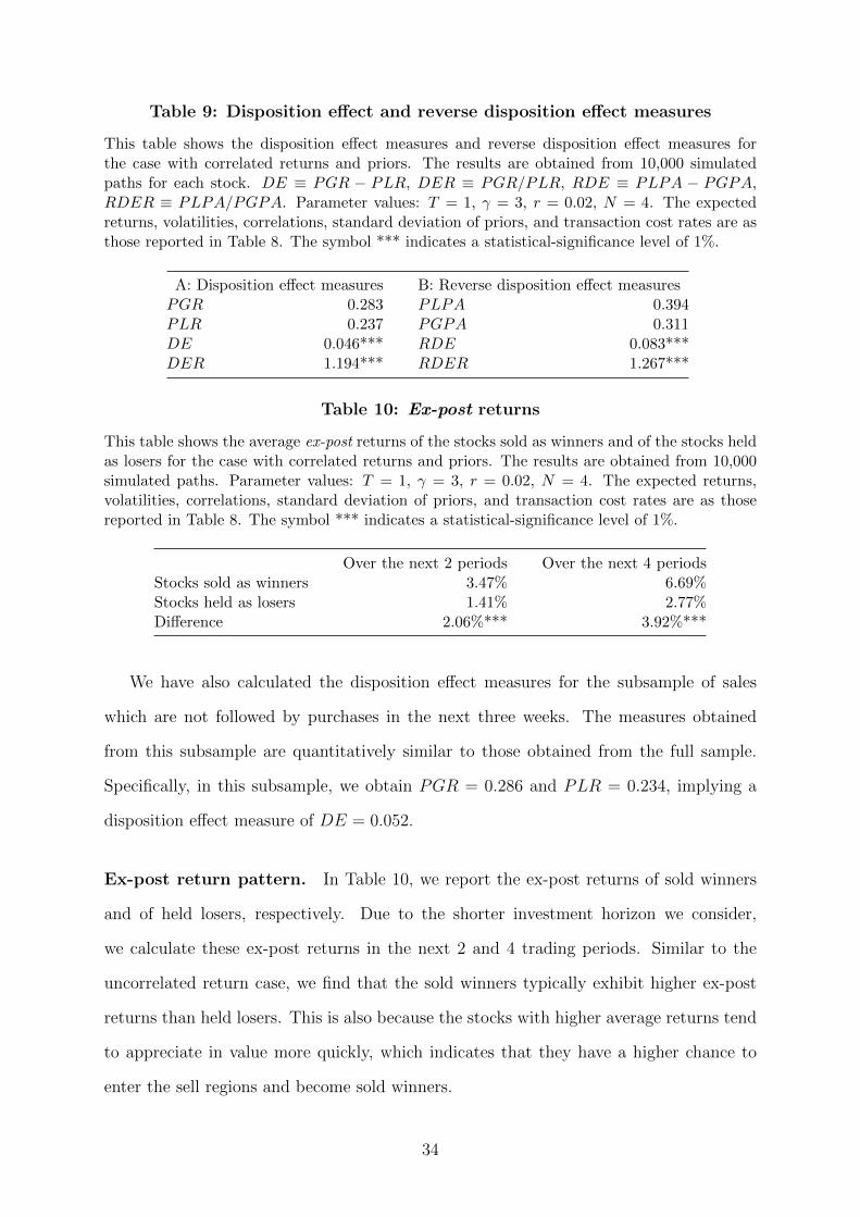
Disposition effect and reverse disposition effect. We report in Table 9 the dispo-
sition effect measures and reverse disposition effect measures we obtain in the correlated
return case. It suggests that the disposition effect still exists in this case. For example,
Panel A reports that PGR equals 0.283 and PLR equals 0.237, implying a disposition
effect measure of DE = 0.046. Similarly, by examining the sample of purchases, we
find that the reverse disposition effect still exists in this model, as shown by the results
reported in Panel B.
Even when the stocks’ returns are correlated, the exposure effect still exists, and the
investor tends to reduce risk exposures after gains and increase risk exposures after losses
on average. The disposition effect and reverse disposition effect are still driven by such
exposure effect.
33
Table 9: Disposition effect and reverse disposition effect measures
This table shows the disposition effect measures and reverse disposition effect measures forthe case with correlated returns and priors. The results are obtained from 10,000 simulatedpaths for each stock. DE ≡ PGR − PLR, DER ≡ PGR/PLR, RDE ≡ PLPA − PGPA,RDER ≡ PLPA/PGPA. Parameter values: T = 1, γ = 3, r = 0.02, N = 4. The expectedreturns, volatilities, correlations, standard deviation of priors, and transaction cost rates are asthose reported in Table 8. The symbol *** indicates a statistical-significance level of 1%.
This table shows the average ex-post returns of the stocks sold as winners and of the stocks heldas losers for the case with correlated returns and priors. The results are obtained from 10,000simulated paths. Parameter values: T = 1, γ = 3, r = 0.02, N = 4. The expected returns,volatilities, correlations, standard deviation of priors, and transaction cost rates are as thosereported in Table 8. The symbol *** indicates a statistical-significance level of 1%.
Over the next 2 periods Over the next 4 periodsStocks sold as winners 3.47% 6.69%Stocks held as losers 1.41% 2.77%Difference 2.06%*** 3.92%***
We have also calculated the disposition effect measures for the subsample of sales
which are not followed by purchases in the next three weeks. The measures obtained
from this subsample are quantitatively similar to those obtained from the full sample.
Specifically, in this subsample, we obtain PGR = 0.286 and PLR = 0.234, implying a
disposition effect measure of DE = 0.052.
Ex-post return pattern. In Table 10, we report the ex-post returns of sold winners
and of held losers, respectively. Due to the shorter investment horizon we consider,
we calculate these ex-post returns in the next 2 and 4 trading periods. Similar to the
uncorrelated return case, we find that the sold winners typically exhibit higher ex-post
returns than held losers. This is also because the stocks with higher average returns tend
to appreciate in value more quickly, which indicates that they have a higher chance to
enter the sell regions and become sold winners.
34
-0.2 -0.1 0 0.1 0.2
Annulized return
0.23
0.24
0.25
0.26
0.27
Pro
ba
bili
ty
A1: Selling, Unobservable case
-0.2 -0.1 0 0.1 0.2
Annulized return
0.16
0.17
0.18
0.19
0.2
0.21
0.22
Pro
ba
bili
ty
B1: Buying, Unobservable case
-0.2 -0.1 0 0.1 0.2
Annulized return
0.17
0.18
0.19
0.2
0.21
0.22
0.23
Pro
ba
bili
ty
A2: Selling, observable case
-0.2 -0.1 0 0.1 0.2
Annulized return
0.1
0.15
0.2
0.25
0.3
0.35
0.4
Pro
ba
bili
ty
B2: Buying, observable case
Figure 5: Probability of selling or of buying shares.This figure shows the probability of selling or of buying shares against the up-to-dateannualized return for the case with correlated returns and priors. Parameter values:T = 1, γ = 3, r = 0.02, N = 4. The expected returns, volatilities, correlations, standarddeviation of priors, and transaction cost rates are as those reported in Table 8. In theobservable case, we set Vi(0) = 0 for i = 1, ..., 4.
V-shaped trading patterns and distribution of realized returns. In Figure 5, we
plot the probability of selling/purchasing shares as a function of past returns. The results
indicate that these probabilities can still both increase as the sizes of gains/losses become
larger. Moreover, the left (right) branch of the V-shape for selling (buying) disappears
when there is no parameter uncertainty (i.e., no learning effect), as shown by Panel A2
(B2).
Intuitively, even when stock returns are correlated, the basic idea that the investor
should decrease (increase) her estimates of expected returns after large negative (positive)
price moves still holds. Thus, the probability of selling shares (of purchasing additional
35
Figure 6: Distribution of realized returns.This figure presents the distribution of realized returns for the case with correlated returnsand priors. Parameter values: T = 1, γ = 3, r = 0.02, N = 4. The expected returns,volatilities, correlations, standard deviation of priors, and transaction cost rates are asthose reported in Table 8.
shares) can still increase as the past return become more negative (positive).32
In the uncorrelated return case, we have shown that the distribution of realized returns
has a humped shape, with a maximal value at the domain of gains. In Figure 6, we show
the distribution of realized returns (on an after-annualization basis) in the correlated
return case, which suggests that the distribution exhibits similar patterns in this case.
The reason is the same as before: the investor optimally keeps her risk exposure in a
certain range, and thus sales are most likely to occur when the magnitude of a gain is
just large enough to push her risk exposure out of the optimal range.
Repurchase effect. In Table 11, we report the repurchase effect measures obtained
from simulations. The results suggest that the investor is still reluctant to repurchase
stocks previously sold for a loss and stocks that have appreciated in price subsequent to
a prior sale. Hence, these repurchase patterns are still consistent with that reported in
32 Note that the probabilities plotted in Figure 5 are generally greater in magnitude than those inFigure 2. This is because we assume lower transaction cost rates and a smaller number of intermediateperiods per year when we numerically solve the model with correlated returns (20 v.s. 250 specifically),which increases the likelihood of trading on each time node.
36
Strahilevitz, Odean, and Barber (2011).
Table 11: Repurchase effect measures
This table shows the repurchase effect measures for the case with correlated returns and priors.The results are obtained from 10,000 simulated paths for each stock. Parameter values: T = 1,γ = 3, r = 0.02, N = 4. The expected returns, volatilities, correlations, standard deviation ofpriors, and transaction cost rates are as those reported in Table 8. The symbol *** indicates astatistical-significance level of 1%.
A: Previous winners or losers B: Winners or losers since last salePLRP 0.200 PDR 0.131PWRP 0.221 PUR 0.079Difference -0.021*** Difference 0.052***
4 Further Discussions
4.1 Disposition effect in the presence of capital gains tax
It is well known that, with capital gains tax and full capital loss tax rebate, loss realization
is beneficial while gains realization becomes more costly (Constantinides (1983)). As a
result, the disposition effect will be reduced if one takes capital gains tax into account.
We have also examined the effect of capital gains tax on the disposition effect. We
focus on the uncorrelated return case and use the same stock-by-stock approximation
approach as previously.33
In Table 12, we report the disposition effect measures obtained in the presence of
capital gains tax. As anticipated, the presence of capital gains tax increases the investor’s
propensity to realize losses and decreases her propensity to realize gains, thus reducing
the disposition effect. However, a significant disposition effect still exists, even with
capital gains tax. For example, with a capital gains tax rate of 20%, the disposition
effect measure DE = 0.058, which is still statistically significant. Meanwhile, our finding
33 To keep the conciseness of the exposition, we relegate to Appendix A.6 the details of the modelwith capital gains tax. Portfolio choice problems with multiple stocks are difficult to solve because ofthe significant increase in the number state variables even after simplifying approximations such averagebasis and full rebate for capital losses (see, e.g., Gallmeyer, Kaniel, and Tompaidis (2006)). Meanwhile,it can be expected that the stock-by-stock approximation is less accurate in the presence of capital gainstaxes.
37
Table 12: Capital gains tax and disposition effect measures
This table reports the disposition effect measure DE = PGR−PLR with/without capital gainstax rates. Parameter values: T = 5, γ = 3, r = 0.026(= 0.04 ∗ (1 − 0.36)), N = 4; µi = 0.1,σi = 0.3, zi0 = 0.1, Vi(0) = 0.0045, and αi = θi = 0.01, for i = 1, ..., N . The symbol ***indicates a statistical-significance level of 1%.
No capital gains tax 10% capital gains tax 20% capital gains taxPGR 0.356 0.320 0.282PLR 0.143 0.182 0.224DE 0.213*** 0.138*** 0.058***DER 2.494*** 1.762*** 1.258***
that the disposition effect measure decreases in tax rate can be consistent with Dhar and
Zhu (2006)’s finding that investors with higher income are less prone to the disposition
effect, because these investors are subject to a higher capital gains tax rate.
It should be noted that we assume that the capital losses are fully rebatable to simplify
our analysis. In practice, however, the U.S. tax code stipulates a limited tax rebate of
up to $3,000 in losses per year. This feature would reduce the benefit of realizing losses,
and thus would increase the magnitude of the disposition effect significantly.
To summarize, although capital gains tax tends to reduce the disposition effect, the
disposition effect is still significant even with capital gains tax. The main intuition is that
the exposure effect is still present and in the presence of transaction costs, it is optimal to
defer even some large capital losses even when capital losses are fully rebatable. Therefore,
the disposition effect is still present, although the magnitude of the disposition effect is
reduced due to the additional benefit of realizing losses and deferring gains.
4.2 A discussion of prospect theory models with learning and
transaction costs
In the existing literature, researchers often use prospect theory preferences (often with
transaction costs) to explain certain investor behaviors including the disposition effect
(e.g., Ingersoll and Jin (2013), Barberis and Xiong (2009)). We next discuss the pos-
sible implications of such a model if it is combined with the learning effect induced by
parameter uncertainty.
38
A decrease in stock price motivates the investor to sell the stock to reset the reference
point. In addition, the learning effect makes the stock less attractive since the estimate
of expected return decreases. Combining these two effects, such a model would predict
that after a decrease in the stock price, the investor tends to sell the stock and buy back
immediately a smaller amount of the stock to maintain an optimal risk exposure. Since
a fall in the price results in a loss more likely, this implication is against the disposition
effect.
If investors also derive utility from realizing gains (e.g., Ingersoll and Jin (2013),
Barberis and Xiong (2009)), an increase in the stock price motivates the investor to sell
the stock to obtain realization utilities. On the other hand, the learning effect makes
the stock more attractive since her estimate of the expected return increases. Combining
these two effects, such a model would predict that after an increase in the stock price,
the investor tends to sell the stock and then repurchase a larger amount of the stock
immediately. Since an increase in the price results in a gain more likely, this implication
is consistent with the disposition effect.
In both cases, the predictions are different from those of our portfolio rebalancing
model, which implies that the investor will either sell or buy some stock shares, but
not both, depending on the relative strength of the exposure effect versus the learning
effect. In addition, after a decrease in the stock price, the learning effect in our model is
counteracted against by another effect (i.e., the exposure effect), while the learning effect
in a prospect utility model is magnified by the reference point resetting effect.
5 Conclusions
The disposition effect, i.e., the tendency of investors to sell winners while holding onto
losers, has been widely documented. Most of the existing theories that attempt to explain
the disposition effect (mostly based on prospect theory, mental accounting, and regret
aversion) cannot explain why the plots of the probabilities of buying more and of selling
against paper profit both exhibit V-shape patterns, as shown by Ben-David and Hirsh-
39
leifer (2012). In addition, they are largely silent on other well-documented disposition-
effect related patterns, such as investors selling winners that subsequently outperform
losers that they hold, the disposition effect being greater for stocks with greater volatili-
ties, and the disposition effect being stronger for less sophisticated investors.
Based on the empirical evidence on the relevance of portfolio rebalancing, learning,
and transaction costs for retail investors who typically hold a small number of stocks,
we propose an optimal portfolio rebalancing model with learning and transaction costs
to show that the disposition effect and many of the related patterns, including the V-
shaped trading patterns, are consistent with the optimal trading strategies implied by
The contents of this appendix are arranged as follows. In Section A.1, we describe the
numerical method for solving the case with uncorrelated returns and priors. In Section
A.2, we provide a quantitative discussion of the learning effect in the uncorrelated case.
In Section A.3, we describe the numerical method for solving the case with correlated
returns and priors. In Section A.4, we show that a model with only four stocks (the
median stockholding number in Odean (1998)’s sample) is not able to generate disposition
effect measures close to the empirical magnitude. In Section A.5, we provide details for
the calculation of the probabilities of selling and buying. In Section A.6, we present the
model with capital gains tax.
A.1 Numerical Method for the Case with Uncorre-
lated Returns and Priors
When stock returns and priors for risk premia are all uncorrelated, we design a trading
strategy which is economically intuitive and is a good approximation to the optimal.
First, in this case, the volatility matrix is σ = diag(σ1, ..., σN) and the covariance matrix
of priors is ∆ = diag(V1(0), ..., VN(0)). Thus, we have P = I (identity matrix) and
di = Vi(0), which implies δi(t) = Vi(0)1+Vi(0)t
. Let zit = E[µi|Ft] = r + ξi(t)σi and Vi(t) =
E[(µi − zit)2|Ft], then it is easy to show that
dzit = σzi(t)dBit, (A-1)
where σzi(t) = Vi(t)σi
, Vi(t) satisfies:
dVi(t)
dt= −
(Vi(t)
σi
)2
, (A-2)
45
and Bit is defined as follows:
dBit =1
σi(µi − zit)dt+ dBit. (A-3)
To illustrate the approximation idea, we first show that, under the independence
assumption, the optimal position in each stock can be independently solved when the
transaction cost is absent.
Proposition 1: (Decomposition of risk exposure in the absence of transaction cost) Sup-
pose that there is no transaction cost for any stock, i.e., αi = θi = 0 for i = 1, 2, ..., N .
Then, the optimal fraction of total wealth Wt invested in Stock i in the model with N
stocks equals the optimal fraction when the investor can only invest in the risk-free asset
and Stock i.
Proof. In the absence of transaction cost, we can choose the investor’s wealth Wt, instead
of (Xt, Y1t, ..., YNt), as a state variable. The budget constraint on Wt is given by:
dWt = Wt
(rdt+
N∑i=1
πit(zit − r)dt+ πitσidBit
), (A-4)
where πit is the fraction of total wealth invested in Stock i at time t, satisfying πit ≥ 0
due to the short-sale constraint. Let Φ(W, z1, ..., zN , t) be the value function, then the
associated HJB equation is:
supπi≥0,1≤i≤N
{∂Φ
∂t+ (r +
N∑i=1
(zi − r)πi)W∂Φ
∂W+
1
2
N∑i=1
π2i σ
2iW
2 ∂2Φ
∂W 2
+1
2
N∑i=1
σzi(t)2∂
2Φ
∂z2i
+W
N∑i=1
πiσiσzi(t)∂2Φ
∂W∂zi
}= 0, (A-5)
with the following terminal condition:
Φ(W, z1, ..., zN , T ) =1
1− γW 1−γ. (A-6)
46
Due to the homogeneity property of the CRRA preference and the linearity of Equation
(A-4), there exists a function h(z1, ..., zN , t), such that:
Φ(W, z1, ..., zN , t) =W 1−γ
1− γe(1−γ)(r(T−t)+h(z1,...,zN ,t)). (A-7)
By substitution, it is straightforward to show that h(z1, ..., zN , t) satisfies the following
equation:
supπi≥0,1≤i≤N
{∂h
∂t+
N∑i=1
((zi − r)πi −
γ
2π2i σ
2i
)+
N∑i=1
(πiσiσzi(t)(1− γ))∂h
∂zi
+1
2
N∑i=1
σzi(t)2
(∂2h
∂z2i
+ (1− γ)
(∂h
∂zi
)2)}
= 0, (A-8)
with a terminal condition:
h(z1, ..., zN , T ) = 0. (A-9)
Now, suppose there are N functions hi(zi), i = 1, ..., N , satisfying the following equation:
supπi≥0
{∂hi
∂t+ (zi − r)πi −
γ
2π2i σ
2i + (πiσiσzi(t)(1− γ))
∂hi
∂zi
+1
2σzi(t)
2
(∂2hi
∂z2i
+ (1− γ)
(∂hi
∂zi
)2)}
= 0, (A-10)
with a terminal condition:
hi(zi, T ) = 0. (A-11)
DefineH(z1, ..., zN , t) =∑N
i=1 hi(zi, t), then it is easy to verify that H(z1, ..., zN , t) satisfies
Equation (A-8), and hence we have:
h(z1, ..., zN , t) =N∑i=1
hi(zi, t). (A-12)
47
Therefore, the optimal allocation to Stock i is given by:
πi(t, zit) =
(zi − r + (1− γ)σiσzi(t)
∂hi
∂zi(zit, t)
γσ2i
)+
, (A-13)
which only depends on the instantaneous estimate of Stock i’s expected return, i.e., zit,
and the calendar time t.
Proposition 1 suggests that, in the absence of transaction cost, if the stocks’ return
processes and priors for risk premia are all independent, then we can decompose the
optimal investment problem with N stocks into N optimal investment problems with a
single stock. This result makes it feasible and reliable to solve for the optimal trading
strategy for a large number of stocks. Motivated by this result, we perform the same
decomposition in the presence of small transaction costs. More specifically, for any stock,
we solve a model with this particular stock and one risk-free asset to compute the in-
vestor’s optimal fraction of wealth invested in this stock in the presence of transaction
cost. We use the obtained optimal fraction in this one-stock model to approximate the
optimal fraction of total wealth in the N -stock model. Although the optimal fraction
obtained in the one-stock model is suboptimal for the N -stock model, it is nevertheless
a good approximation when the transaction cost rates are reasonably small.34
A.2 Learning with Uncorrelated Returns and Priors
In this section, we provide a quantitative discussion of the learning effect in the case
with uncorrelated returns and priors. Note that Equation (A-3) implies the following
34 In an earlier version of the paper, we solved the optimal trading strategy for the same model, but withCARA preferences. We obtained the same qualitative and similar quantitative results on the dispositioneffect-related patterns, because the key driving forces remain the same. We have also computed theoptimal trading strategy in a two-stock case, in which one stock has an observable constant expectedreturn, and found that the results obtained from the approximately optimal strategy are indeed closeto those obtained from the optimal strategy. We do not report these calculations in the paper to savespace. They are, however, available from the authors upon request.
48
stock-price process observed in the investor’s filter:
dSitSit
= zitdt+ σidBit. (A-14)
The solution to Equation (A-2) is:
Vi(t) =σ2i Vi(0)
σ2i + Vi(0) t
, (A-15)
hence, Equation (A-1) becomes:
dzit =σiVi(0)
σ2i + Vi(0) t
dBit, (A-16)
which is equivalent to:
dzit =Vi(0)
σ2i + Vi(0) t
(dSitSit− zitdt
). (A-17)
Since Vi(0)
σ2i +Vi(0)t
> 0, Equation (A-17) suggests that the changes in zit (i.e., the investor’s
conditional expectation of µi) are driven by the instantaneous realized return dSit/Sit in
excess of the current estimate of the expected return zitdt. In particular, the investor will
increase her estimate of the stock’s expected return if and only if:
dSitSit
> zitdt. (A-18)
In other words, a realized return that is better (worse) than the expected return makes
the investor increase (decrease) her estimated expected return.
49
A.3 Numerical Method for the Case with Correlated
Returns and Priors
Our numerical algorithm for this case is based on the deep neural network (DNN) tech-
nique (see, e.g., Han and E (2016), Zhang and Zhou (2019)). Specifically, we extend the
existing algorithm to incorporate parameter uncertainty.
We first present a discrete time version of our model. To do so, we discretize the time
horizon [0, T ] into M subperiods by 0 = t0 < t1 < t2 < · · · < tM = T . We denote the
time length between two time points by h = TM
.
Implementing the deep learning method for the investor’s problem in our model in-
volves two steps at every time point ti. First, we apply the feedforward neutral networks
method to determine the optimal vector of dollar values that the investor should trade
for each stock (the method of calculating this vector is presented shortly). Denoting this
vector by ati ∈ RN , we can write down the following portfolio rebalancing equation:
Xti+ = Xti− −∑N
j=1(1 + θj) (ati)+j +
∑Nj=1(1− αj) (ati)
−j ,
Yti+ = Yti− + ati ,
ξ(ti+) = ξ(ti−),
(A-19)
where ti− (ti+) denotes the time before (after) rebalancing at time ti, (ati)j denotes the
jth element of the trading amount vector ati , and a+ = max{0, a} (a− = max{0,−a})
denotes the positive (negative) part of a.
After the rebalancing step, we apply the Euler-Maruyama scheme to implement the
dynamics of (11), (12) and (13). From time ti+ to ti+1−, we have the dynamics
Xti+1= Xti+ + rhXti+,
(Yti+1−)j = (Yti+)j + (Yti+)j
[rh+ σj · ξ(ti+)h+ σj ·∆Bti
],
ξ(ti+1−) = ξ(ti+) + P ′D(ti)P∆Bti .
(A-20)
50
Combining (A-19) and (A-20) yields the dynamics of the state variables in our model.
At each time point, we set an independent neural network with one input layer, two
hidden layers and one output layer. Our input vector is an N + 1 dimensional vector
including the initial positions in bond and N stocks. Hidden layer one is regarded as a
map to transform the input vector from RN+1 to Rd1 , where d1 is the dimension of the
hidden layer one. The explicit form of hidden layer one is
H1 = f1(X) = ReLu(W1 ·X + b1), (A-21)
where X ∈ RN+1 denotes the input vector, W1 ∈ Rd1×(N+1), b1 ∈ Rd1 are trainable
weights in this layer, and ReLu(x) = x+ is the activation function. Similarly, we specify
the form of the hidden layer two as follows:
H2 = f2(H1) = ReLu(W2 ·H1 + b2), (A-22)
where W2 ∈ Rd2×d1 and b2 ∈ Rd2 . In the output layer, we remove the ReLu function so
that the network can sell stocks as well. Therefore, the output layer can be characterized
by
ati = f3(H2) = W3 ·H2 + b3, (A-23)
where W3 ∈ RN×d2 and b3 ∈ RN . The structure of a single deep neural network is shown
in Figure 7.
The whole computational graph of deep neural networks is shown in Figure 8. After
obtaining the result from the (M − 1)th network, we can then define the following loss
function of the deep neural networks:
L(Θ) = − 1
m
m∑k=1
u
(XΘT,k +
N∑j=1
((1− αj)Y j,Θ
T,k
)), (A-24)
51
Figure 7: Structure of a single deep neural network.
Figure 8: Computational graph of deep neural networks.
52
where Θ denotes the set of all the patameters in this neural networks model, m denotes
the size of our training batch, and u is the investor’s CRRA utility function. We can
update the estimate of Θ by minimizing the loss function. The whole process can be
summarized in Algorithm 1 below.
Algorithm 1 Deep learning algorithm for solving for the optimal strategy
Input: X0, Y0
Require: m, M% Build the innovation process and initialize the neural networks.for i in 0, 1, · · · ,M − 1 do
for j in 1, 2, · · · ,m doSimulate the innovation process (a standard Brownian motion) Bt.
end forObtain trading strategy through the i−th neural networks.Rebalance the portfolio using (A-19).Update Xti+1
, Yti+1, ξ(ti+1) using (A-20).
end forCalculate the loss function L(Θ).Update the parameter set Θ.Output: (XT , YT ) and optimal trading strategies {ati}M−1
i=0
A.4 Number of Stocks and Disposition Effect Mea-
sures
In this section, we show that using a model (either rational or behavioral) with four
stocks, one cannot obtain disposition effect measures which are close in magnitude to
those reported in Odean (1998), even though four stocks is the median stock holding in
Odean (1998)’s sample. For this purpose, we establish the following proposition:
Proposition 2: (Bounds on the disposition effect measures) Suppose every investor holds
N stocks in her portfolio, then at least one of PGR and PLR is no less than 1N
.
Proof. First recall that paper gains, realized gains, paper losses, and realized losses will
only be counted on days when at least one stock is sold. On these days, with probability
one, a sale will be either a realized gain or a realized loss. This is because the set that
53
selling price exactly equals purchase price has a measure of zero. In addition, there can
be at most N − 1 stocks with unrealized paper gains or paper losses when at least one
According to Proposition 2, in a model with four stocks, at least one of PGR and
PLR will be no less than 0.25. Thus Odean (1998)’s finding that PGR = 0.148 and
PLR = 0.098 cannot be matched.
54
A.5 Calculation of Probability of Selling and Buying
To calculate the probability of selling or buying shares of any stock within certain ranges
of realized return, we first choose a realized return bracket [Rmin, Rmax] and divide it into
equally spaced subintervals, so that Rmin = R0 < R1 < ... < Rn = Rmax. We simulate
daily price data for each stock, and perform the following calculations: along each sample
path ω, for each day t when a particular stock i is in the investor’s portfolio, we compute
the annualized continuously compounded return, Retit(ω), obtained by holding this stock
by:
Retit(ω) =1
Hit(ω)log
(Sit(ω)
Ait(ω)
),
where Sit(ω) is the spot price of this stock, Ait(ω) is the average purchase price of this
stock, and Hit(ω) is the average holding time of this stock, all up to day t.35
We define three indicator functions for the corresponding events as follows:
sjit(ω) = 1{Stock i is sold on day t and Rj≤Retit(ω)<Rj+1},
bjit(ω) = 1{More of Stock i is bought on day t and Rj≤Retit(ω)<Rj+1}
and:
Rjit(ω) = 1{Rj≤Retit(ω)<Rj+1}.
We then calculate the frequency:
fSj =
∑i,t,ω s
jit(ω)∑
i,t,ω Rjit(ω)
(A-27)
35 Because multiple purchases and sales of the same stock can occur along a sample path, we usethe average holding time to annualize the returns to make them more comparable. To understand themechanism of the average holding time system, consider the following simple example: assume on day 1,the investor purchases 10 shares; on day 11, the investor purchases five more shares. Then, the averageholding time of each share is (10 × (11 − 1) + 5 × 0)/(10 + 5) = 6.67 days on day 11. Assume that theinvestor does not make any transaction between day 12 and 15, then on day 15, the average holding timeis (10× (15− 1) + 5× (15− 11))/(10 + 5) = 10.67 days.
55
as the probability that a sale takes place with the realized return in the jth bracket, and
similarly:
fBj =
∑i,t,ω b
jit(ω)∑
i,t,ω Rjit(ω)
, (A-28)
as the probability that a purchase takes place with the realized return in the jth bracket.
A.6 A Model with Capital Gains Taxes
In the presence of (fully rebatable) capital gains tax, we need to keep tracking the total
costs of purchasing each stock. Let Kit be the total costs of purchasing Stock i up to
time t, the investor’s budget constraints then read:
is the total proceeds that the investor would obtain if she sold the entire position on
Stock i at time t, and τ is the capital gains tax rate. Therefore, the investor’s time t net
wealth is:
Wt = Xt +N∑i=1
f(Yit, Kit). (A-33)
The investor’s problem is again to choose her optimal policy {(Lit, Iit) : i = 1, ..., N}
among all of the admissible policies to maximize her expected CRRA utility from the
terminal net wealth at some finite time T , i.e.:
E
[W 1−γT
1− γ
], (A-34)
56
0 0.5 1 1.5 2 2.5 3
Basis-price ratio
0
0.05
0.1
0.15
0.2
0.25
0.3
0.35
0.4
Sto
ck a
llocation
SR
NTR
WSR
WSR
C
D
B
SR
BR
A
F
E GNTR
BR
Gain Loss
Figure 9: Trading strategy with capital gains tax.This figure shows a snapshot of the trading boundaries at time t = 2.5 years in thepresence of capital gains tax with fully rebatable capital losses. The region labeled“WSR” is the wash-sale region. Parameter values: T = 5, γ = 3, r = 0.026(= 0.04×0.65),µ1 = 0.1, σ1 = 0.3, V1(0) = 0.0045, and α1 = θ1 = 0.01. The conditional estimate of thereturn predictor is set at z1 = 0.1, and the capital gains tax rate is τ = 0.2.
subject to Equations (11), (A-29), and (A-30), and (A-31), and the short-sale constraint
as well as the solvency condition.
Trading strategy. We plot the trading boundaries for Stock 1 against the basis-price
ratio k1(1−α1)y1
in Figure 9, where k1 is the total cost basis of Stock 1, fixing the estimate
of the expected return at its true value z1 = µ1 and assuming a capital gains tax rate of
15%.36 Note that there is a gain after liquidation if and only if k1(1−α1)y1
< 1. As in the
case without capital gains tax, the investor should maintain the stock exposure within a
certain range, as suggested by the Sell Region (SR) above the sell boundary and the Buy
Region (BR) below the buy boundary.
In contrast to the case with capital gains tax but without transaction costs (as con-
sidered by the existing literature, e.g., Constantinides (1983)), Figure 9 shows that it
can be optimal to defer the realization of even large capital losses, as indicated by the
36 In fact, this plot applies to each stock because they are assumed to have same parameter values.
57
no-transaction region (NTR) to the right of the vertical line at k1(1−α1)y1
= 1. In addition,
even when it is optimal to realize capital losses, the optimal realization can be only a
fraction of the losses, e.g., point A to point B. This is because the time value of the tax
rebate can be smaller than the transaction costs required, and realizing only part of the
losses can avoid the transaction costs needed for buying back shares. Only when the
capital losses are large enough does the investor immediately realize all losses and buy
back some shares to achieve the optimal risk exposure (e.g., point C to point D, and then
to point E).
Due to the presence of transaction costs, when the investor has capital losses, it can
be optimal to purchase more without first realizing losses (e.g., from F to G). This is
because capital loss on a stock reduces the exposure to this stock, and selling first to
realize losses and then buying back some to achieve the desired exposure would incur
too much transaction cost. In such a case, the investor purchases shares to maintain a
desirable exposure to the stock without engaging in any loss selling.