84
Chapter 9 A Real Intertemporal Model with Investment

Chapter 9
A Real Intertemporal Model with Investment
Copyright © 2005 Pearson Addison-Wesley. All rights reserved. 9-2
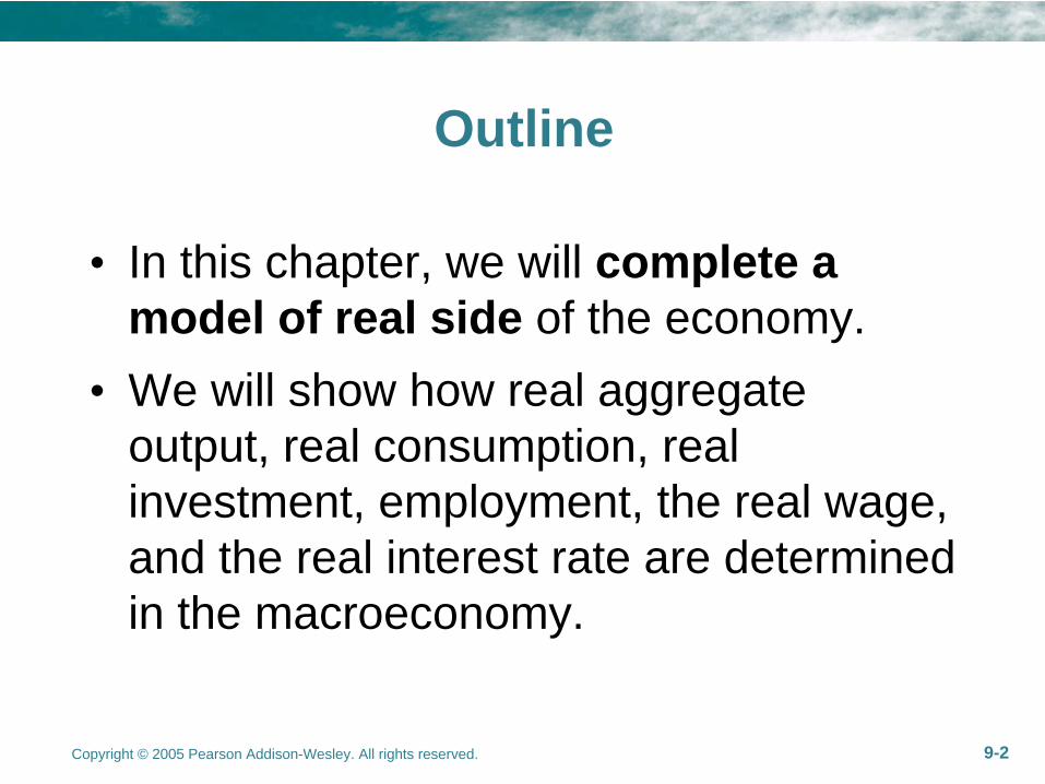
Outline
•
In this chapter, we will complete a model of real side of the economy.
•
We will show how real aggregate output, real consumption, real investment, employment, the real wage, and the real interest rate are determined in the macroeconomy.

Copyright © 2005 Pearson Addison-Wesley. All rights reserved. 9-3
Outline
•
In this model we will bring together the work-leisure choice form Chapter 4 with the intertemporal consumption behavior (consumption-saving decision) from Chapter 8.

Copyright © 2005 Pearson Addison-Wesley. All rights reserved. 9-4
The Representative Consumer
•
Utility function
•
Current BC
( , ', , ')U CC l l
( )pC S wh l T
Copyright © 2005 Pearson Addison-Wesley. All rights reserved. 9-5
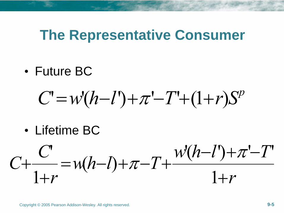
The Representative Consumer
•
Future BC
•
Lifetime BC
' '( ') ' ' (1 ) pC w h l T r S
' '( ') ' '( )1 1C w h l TC wh l Tr r

Copyright © 2005 Pearson Addison-Wesley. All rights reserved. 9-6
•
Representative consumer’s problem
Subject to lifetime BC
, ', , 'max ( , ', , ')C C l l U C C l l

Copyright © 2005 Pearson Addison-Wesley. All rights reserved. 9-7
•
FOCs
,' 1
',' 1
U UC C rU U wwl l r

Copyright © 2005 Pearson Addison-Wesley. All rights reserved. 9-8
The Optimization Conditions
.
'. '
. '
//
/ ' '/ '/ 1/ '
l C
l C
C C
U lMRS wU CU lMRS wU CU CMRS rU C
Copyright © 2005 Pearson Addison-Wesley. All rights reserved. 9-9
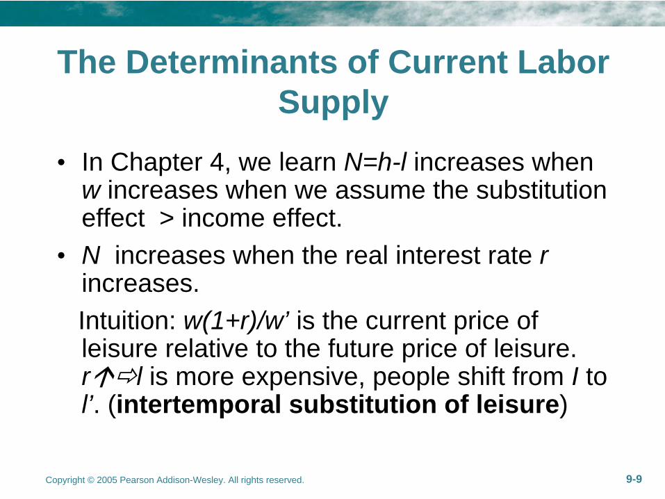
The Determinants of Current Labor Supply
•
In Chapter 4, we learn N=h-l increases when w increases when we assume the substitution effect > income effect.
•
N increases when the real interest rate r increases.Intuition: w(1+r)/w’ is the current price of leisure relative to the future price of leisure. rl is more expensive, people shift from I to l’. (intertemporal substitution of leisure)

Copyright © 2005 Pearson Addison-Wesley. All rights reserved. 9-10
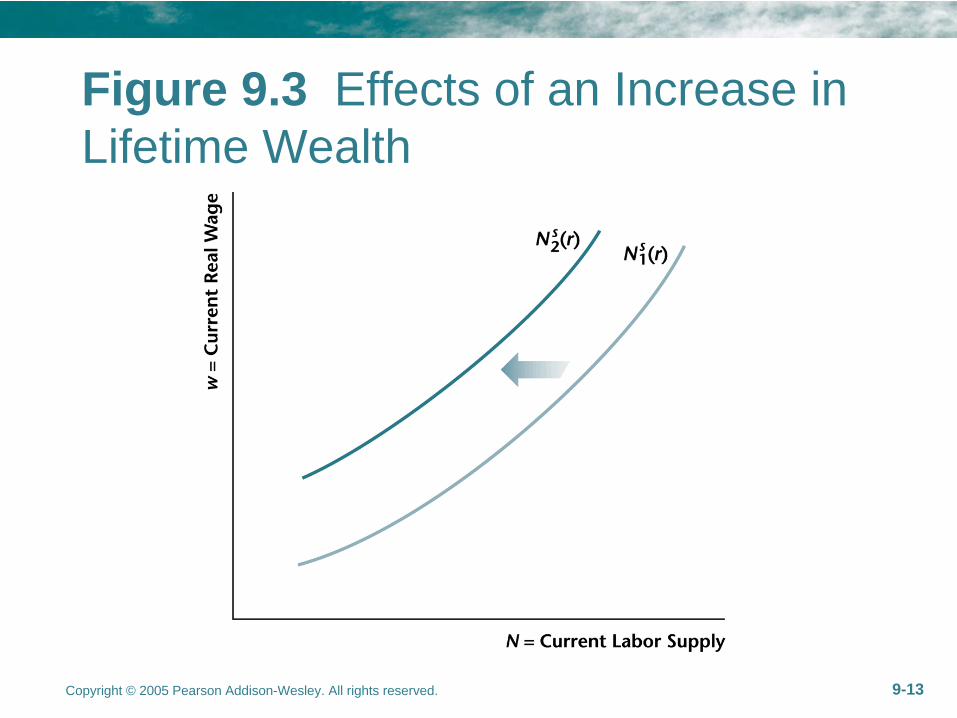
•
N decreases when the lifetime wealth increases.Intuition: because leisure is the normal good.

Copyright © 2005 Pearson Addison-Wesley. All rights reserved. 9-11
Figure 9.1 The Representative Consumer's Current Labor Supply Curve

Copyright © 2005 Pearson Addison-Wesley. All rights reserved. 9-12
Figure 9.2 An Increase in the Real Interest Rate Shifts the Current Labor Supply Curve to the Right
Copyright © 2005 Pearson Addison-Wesley. All rights reserved. 9-13
Figure 9.3 Effects of an Increase in Lifetime Wealth
Copyright © 2005 Pearson Addison-Wesley. All rights reserved. 9-14
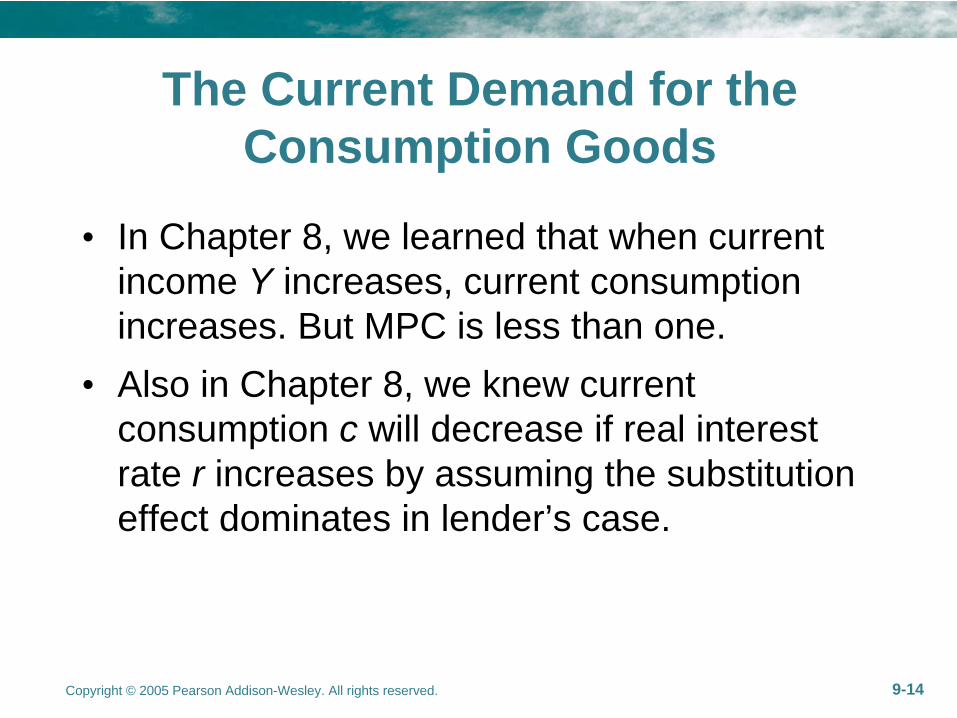
The Current Demand for the Consumption Goods
•
In Chapter 8, we learned that when current income Y increases, current consumption increases. But MPC is less than one.
•
Also in Chapter 8, we knew current consumption c will decrease if real interest rate r increases by assuming the substitution effect dominates in lender’s case.

Copyright © 2005 Pearson Addison-Wesley. All rights reserved. 9-15
•
Holding constant Y and r, if lifetime wealth increases, current consumption increases by income effect.

Copyright © 2005 Pearson Addison-Wesley. All rights reserved. 9-16
Figure 9.4 The Representative Consumer's Current Demand for Consumption Goods Increases with Income
Copyright © 2005 Pearson Addison-Wesley. All rights reserved. 9-17
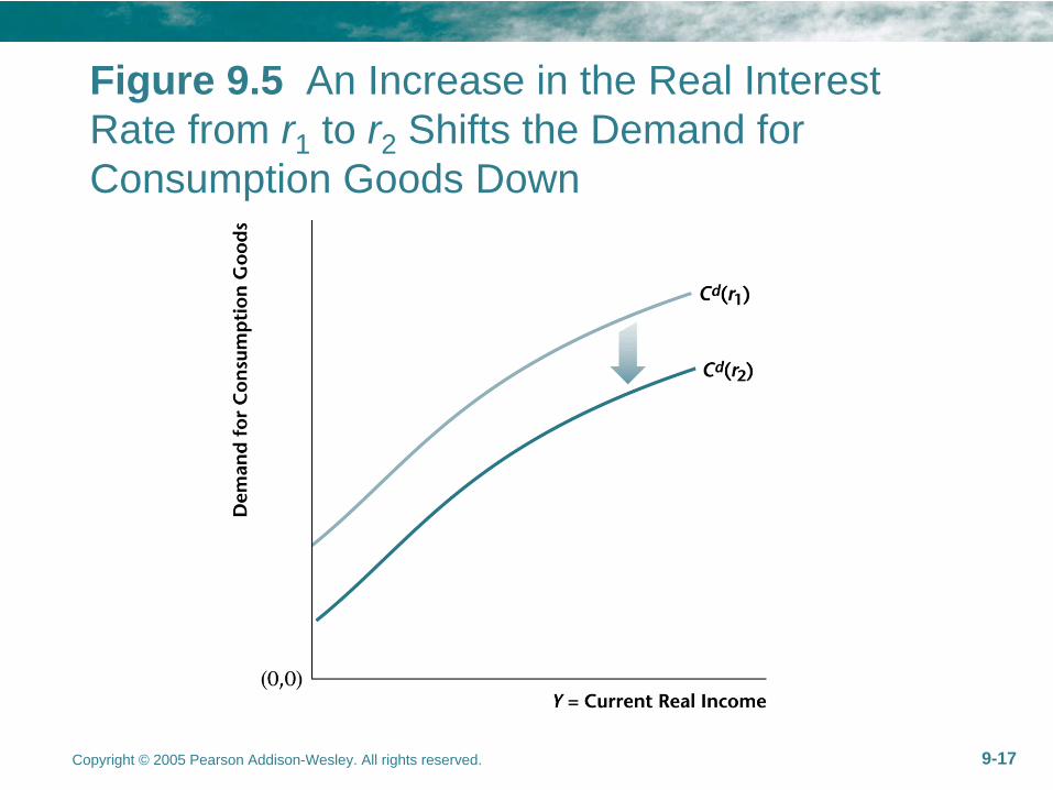
Figure 9.5 An Increase in the Real Interest Rate from r1 to r2 Shifts the Demand for Consumption Goods Down

Copyright © 2005 Pearson Addison-Wesley. All rights reserved. 9-18
Figure 9.6 An Increase in Lifetime Wealth for the Consumer Shifts Up the Demand for Consumption Goods.
Copyright © 2005 Pearson Addison-Wesley. All rights reserved. 9-19
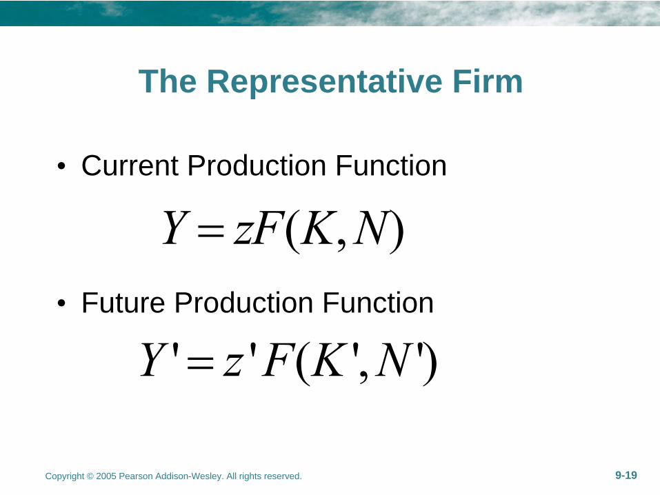
The Representative Firm
•
Current Production Function
•
Future Production Function
( , )Y zF K N
' ' ( ', ')Y z F K N
Copyright © 2005 Pearson Addison-Wesley. All rights reserved. 9-20
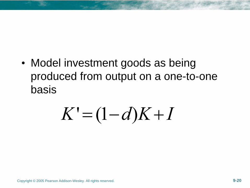
•
Model investment goods as being produced from output on a one-to-one basis
' (1 )K d K I
Copyright © 2005 Pearson Addison-Wesley. All rights reserved. 9-21
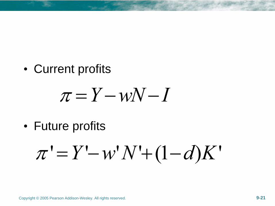
•
Current profits
•
Future profits
Y wN I
' ' ' ' (1 ) 'Y w N d K

Copyright © 2005 Pearson Addison-Wesley. All rights reserved. 9-22
•
The Representative Firm’s problem
, ','max
1N N I V r
Copyright © 2005 Pearson Addison-Wesley. All rights reserved. 9-23
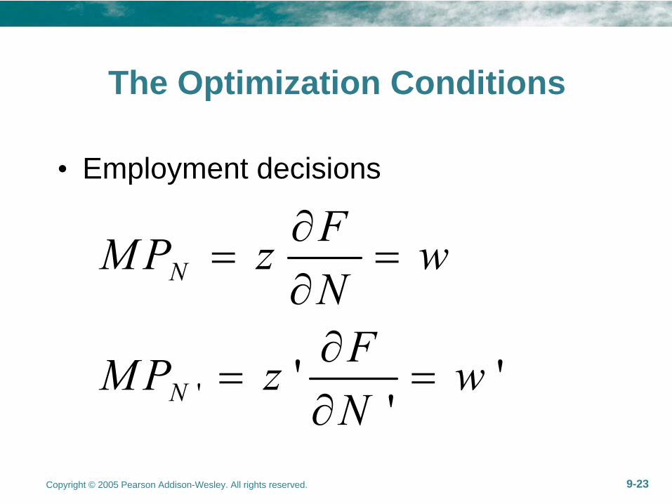
The Optimization Conditions
•
Employment decisions
' ' ''
N
N
FMP z wNFMP z wN
Copyright © 2005 Pearson Addison-Wesley. All rights reserved. 9-24
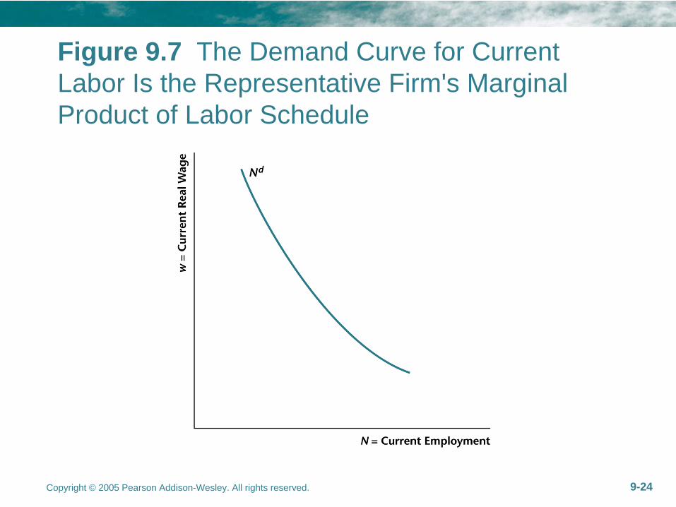
Figure 9.7 The Demand Curve for Current Labor Is the Representative Firm's Marginal Product of Labor Schedule

Copyright © 2005 Pearson Addison-Wesley. All rights reserved. 9-25
Figure 9.8 The Current Demand Curve for Labor Shifts Due to Changes in Current Total Factor Productivity z and in the Current Capital Stock K

Copyright © 2005 Pearson Addison-Wesley. All rights reserved. 9-26
The investment decision
•
The marginal cost of investment
Because when I increases one unit, the present value of profits V decreases one unit accordingly. Hence 1 is the marginal cost of investment.
( ) 1MC I

Copyright © 2005 Pearson Addison-Wesley. All rights reserved. 9-27
•
The marginal benefit from investment
' 1( )1KMP dMB Ir

Copyright © 2005 Pearson Addison-Wesley. All rights reserved. 9-28
•
Firm will equate the marginal benefit and marginal cost of investment
i.e.
' 1 11KMP dr
'KMP d r

Copyright © 2005 Pearson Addison-Wesley. All rights reserved. 9-29
•
Firm will invest until the net marginal product of capital is equal to the real interest rate. This is the optimal investment rule.

Copyright © 2005 Pearson Addison-Wesley. All rights reserved. 9-30
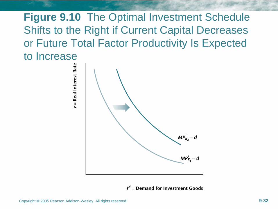
•
Two types of shifts in the optimal investment schedule–
When z’ increases, optimal investment schedule shifts to the right.
–
When K is higher, then optimal investment schedule shifts to the left.
Copyright © 2005 Pearson Addison-Wesley. All rights reserved. 9-31
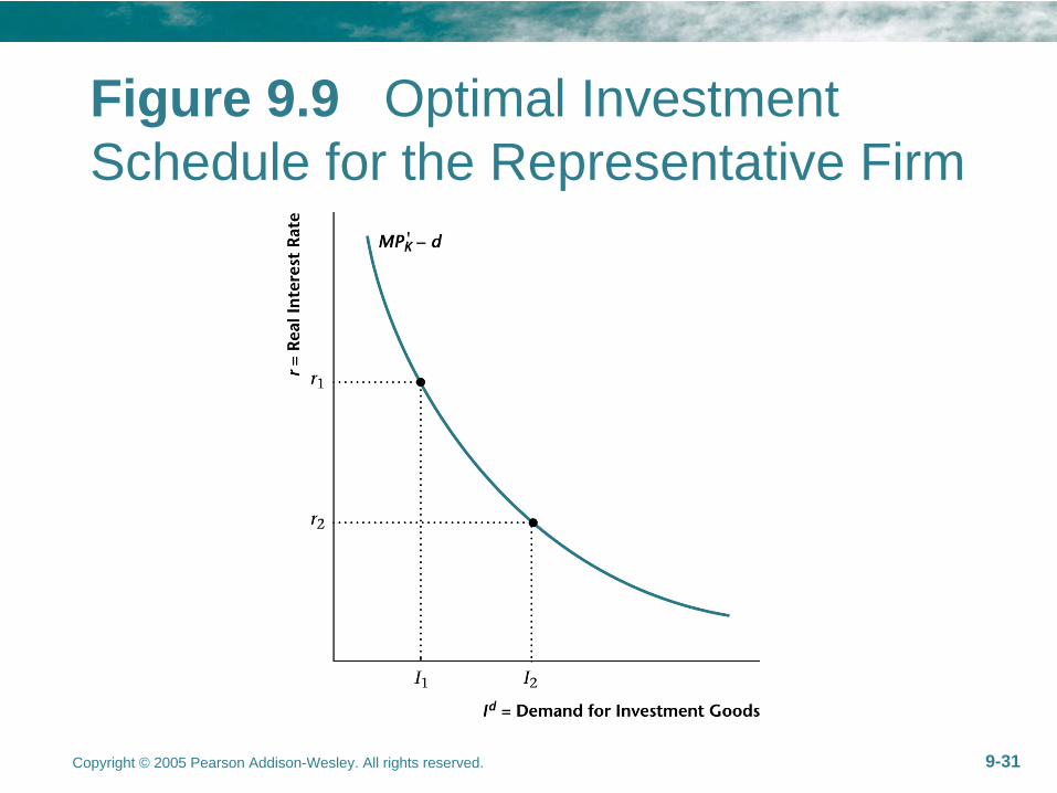
Figure 9.9 Optimal Investment Schedule for the Representative Firm
Copyright © 2005 Pearson Addison-Wesley. All rights reserved. 9-32
Figure 9.10 The Optimal Investment Schedule Shifts to the Right if Current Capital Decreases or Future Total Factor Productivity Is Expected to Increase

Copyright © 2005 Pearson Addison-Wesley. All rights reserved. 9-33
Optimal Investment: A Numerical Example
•
Paula, a small-scale farmer, has an apple orchard. K=10.
•
10 trees can produce 100 bushels of apples. Y=100.
•
At the end of each period, 20% of trees die. d=0.2.
•
The liquidation price is one tree for one bushel of apples.
•
Real interest rate = 5%.
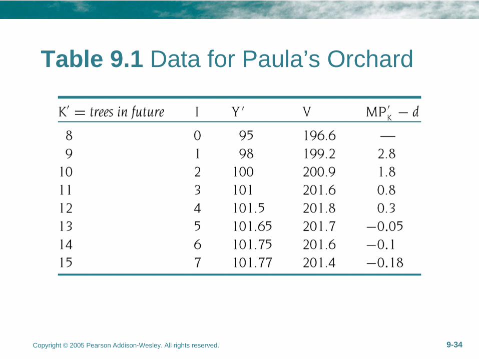
Copyright © 2005 Pearson Addison-Wesley. All rights reserved. 9-34
Table 9.1 Data for Paula’s Orchard

Copyright © 2005 Pearson Addison-Wesley. All rights reserved. 9-35
Government
•
Government has present-value BC
' '1 1G TG Tr r

Copyright © 2005 Pearson Addison-Wesley. All rights reserved. 9-36
Competitive Equilibrium
In this two-period economy, an CE is anallocation (c,c’,s,l,l’) for the representative
consumer, an allocation (N,N’,I) for the representative firm, a policy (G,G’,T,T’) for the government, and a price system (w,w’,r) such that:
•
The consumer chooses c,c’,s,l,l’ optimally given r,w,w’

Copyright © 2005 Pearson Addison-Wesley. All rights reserved. 9-37
Competitive Equilibrium
•
The firm chooses N,N’,I to maximize the lifetime profit V
•
Gov balances its lifetime BC•
Labor market clears: h-l=N, h-l’=N’
•
Good market clears: C+I+G=Y, C’+G’=Y’

Copyright © 2005 Pearson Addison-Wesley. All rights reserved. 9-38
Competitive Equilibrium
•
We will show how a CE, where supply equals demand in the current-period labor and goods markets, can be expressed in terms of diagrams.
Copyright © 2005 Pearson Addison-Wesley. All rights reserved. 9-39
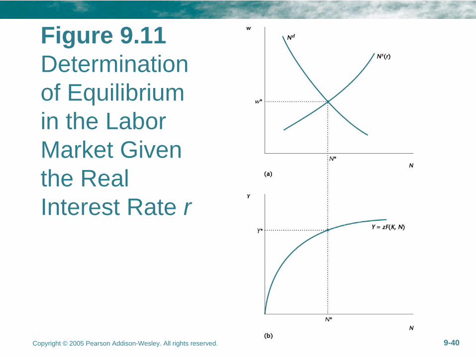
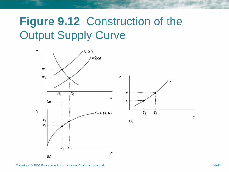
The Current Labor Market and the Output Supply Curve
•
Given real interest rate r, current labor market clears at the current wage w* and the current equilibrium employment N*. Hence the equilibrium current output Y* is determined.
•
When r changes, Y* will change accordingly. We show the relationship in the output supply curve Ys.
Copyright © 2005 Pearson Addison-Wesley. All rights reserved. 9-40
Figure 9.11 Determination of Equilibrium in the Labor Market Given the Real Interest Rate r
Copyright © 2005 Pearson Addison-Wesley. All rights reserved. 9-41
Figure 9.12 Construction of the Output Supply Curve

Copyright © 2005 Pearson Addison-Wesley. All rights reserved. 9-42
•
Slope of Output Supply—Real Interest Rate Effects
•
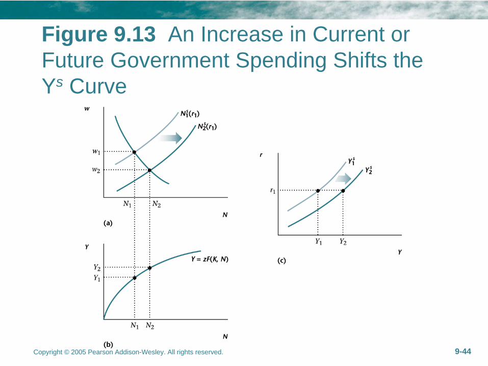
Shifts in Output Supply–
Lifetime Wealth, e.g., an increase in G or G’ will shift labor supply curve to the right and shifts the output supply curve to the right due to the income effect on labor supply. (less income, less leisure)

Copyright © 2005 Pearson Addison-Wesley. All rights reserved. 9-43
–
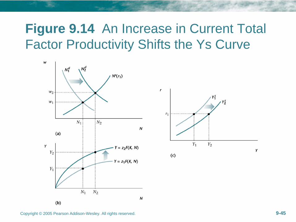
TFP. Increase in z will shift the output supply curve to the right.
–
Capital Stock K. Same as z.
Copyright © 2005 Pearson Addison-Wesley. All rights reserved. 9-44
Figure 9.13 An Increase in Current or Future Government Spending Shifts the Ys Curve
Copyright © 2005 Pearson Addison-Wesley. All rights reserved. 9-45
Figure 9.14 An Increase in Current Total Factor Productivity Shifts the Ys Curve
Copyright © 2005 Pearson Addison-Wesley. All rights reserved. 9-46
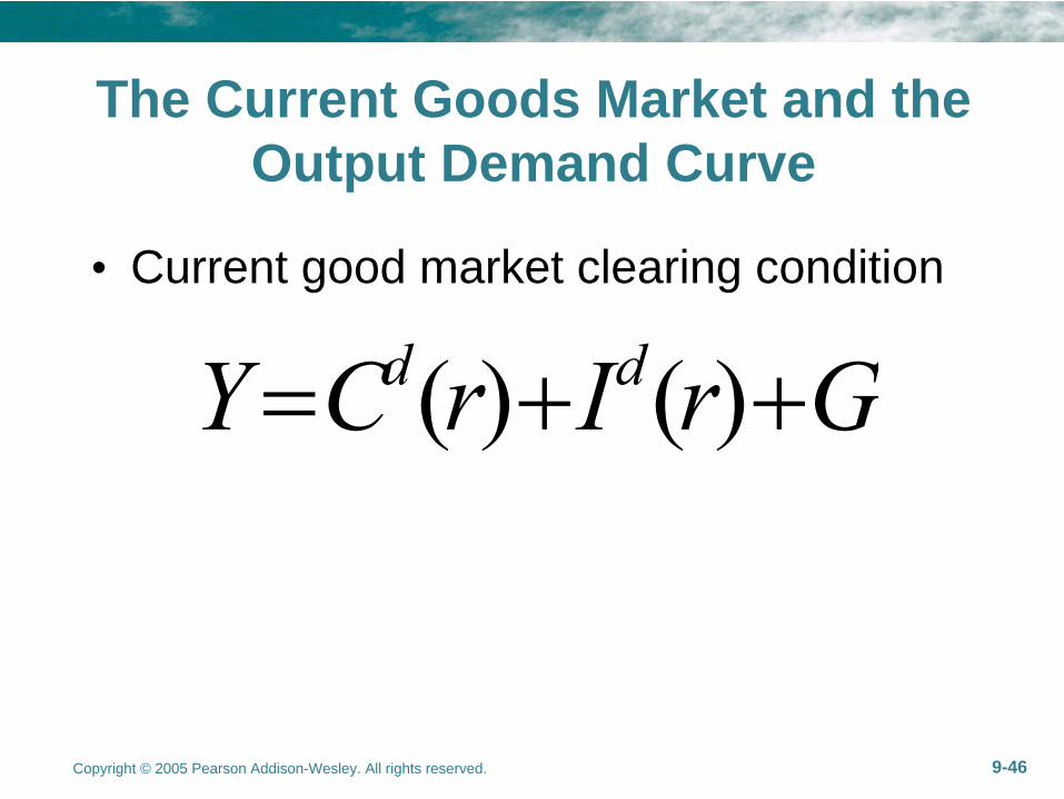
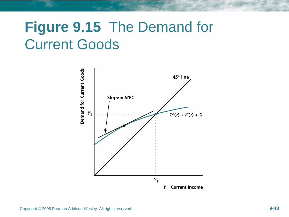
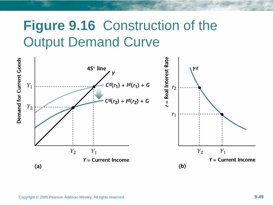
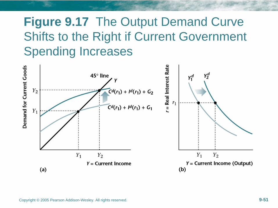
The Current Goods Market and the Output Demand Curve
•
Current good market clearing condition
( ) ( )d dY C r I r G

Copyright © 2005 Pearson Addison-Wesley. All rights reserved. 9-47
•
From this condition, we can trace out the output demand curve Yd as a function of real interest rate r.
•
The slope of Yd is negative.
Copyright © 2005 Pearson Addison-Wesley. All rights reserved. 9-48
Figure 9.15 The Demand for Current Goods
Copyright © 2005 Pearson Addison-Wesley. All rights reserved. 9-49
Figure 9.16 Construction of the Output Demand Curve
Copyright © 2005 Pearson Addison-Wesley. All rights reserved. 9-50
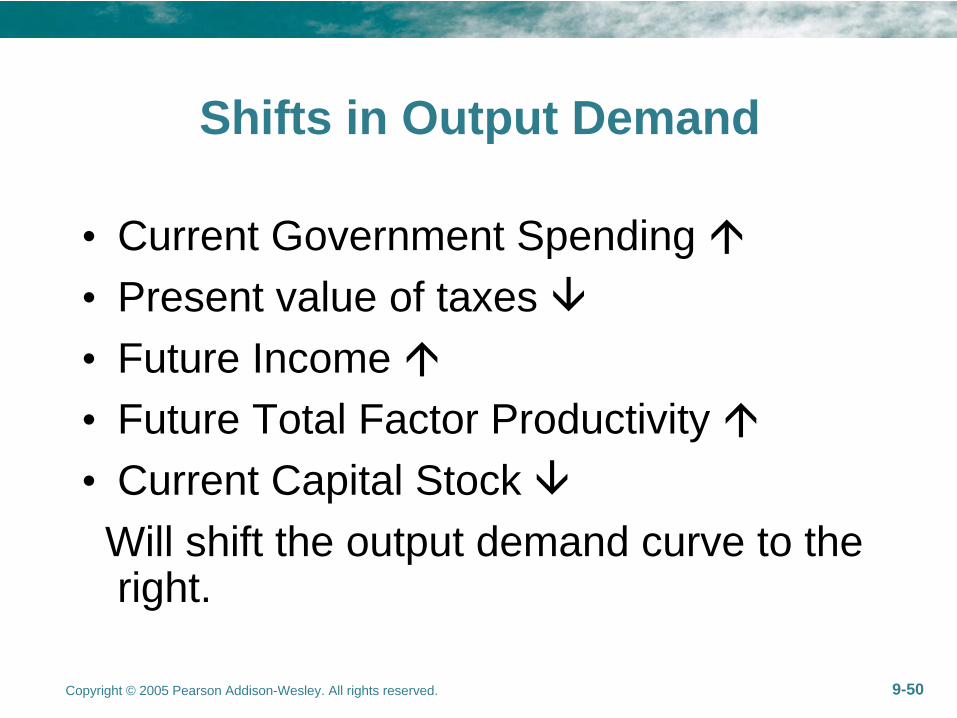
Shifts in Output Demand
•
Current Government Spending •
Present value of taxes
•
Future Income •
Future Total Factor Productivity
•
Current Capital Stock Will shift the output demand curve to the right.
Copyright © 2005 Pearson Addison-Wesley. All rights reserved. 9-51
Figure 9.17 The Output Demand Curve Shifts to the Right if Current Government Spending Increases

Copyright © 2005 Pearson Addison-Wesley. All rights reserved. 9-52
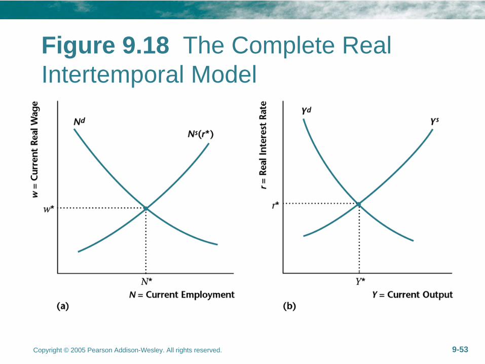
The Complete Real Intertemporal Model
•
Equilibrium in the Labor Market
•
Equilibrium in the Goods Market
( *) *, *d sN N r w N
( ) ( ) *, *d sY r Y r r Y
Copyright © 2005 Pearson Addison-Wesley. All rights reserved. 9-53
Figure 9.18 The Complete Real Intertemporal Model

Copyright © 2005 Pearson Addison-Wesley. All rights reserved. 9-54
Working with the Model
Two key messages in this chapter •
It does matter that whether the shock is temporary or permanent
•
The effects of a shock to the economy expected in the future will have important macroeconomic effects in the current period.We will use several experiments to show them.
Copyright © 2005 Pearson Addison-Wesley. All rights reserved. 9-55
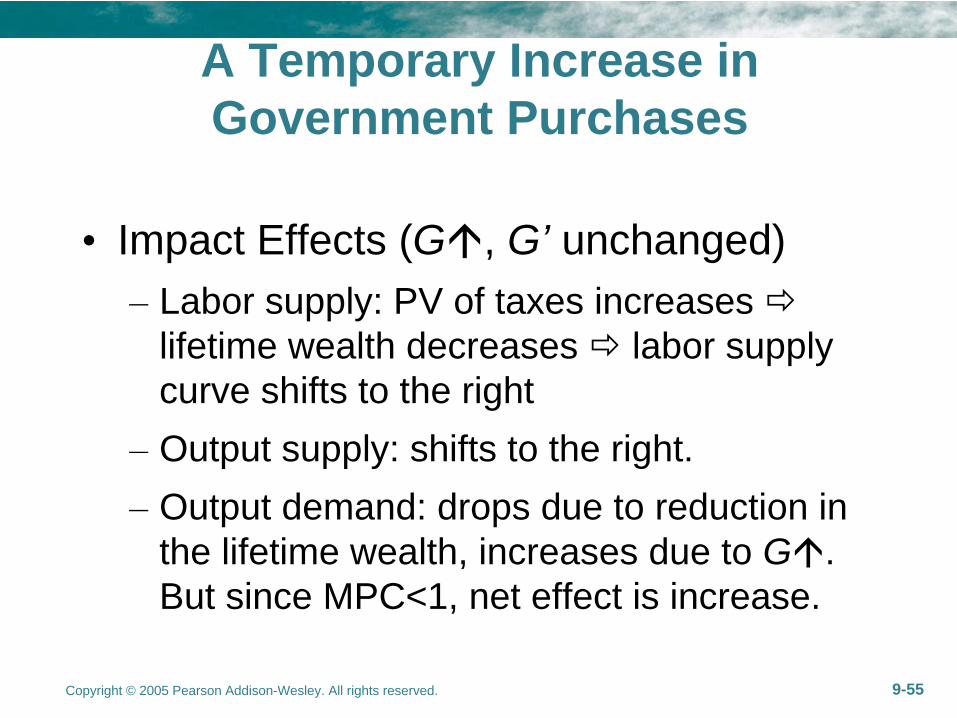
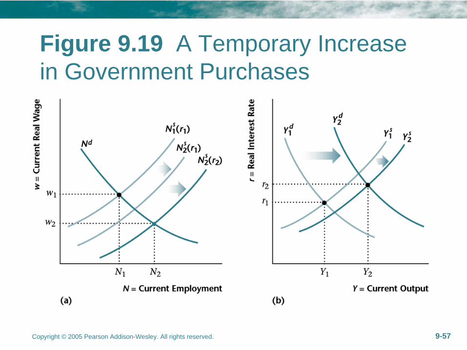
A Temporary Increase in Government Purchases
•
Impact Effects (G, G’ unchanged)–
Labor supply: PV of taxes increases
lifetime wealth decreases
labor supply curve shifts to the right
–
Output supply: shifts to the right.–
Output demand: drops due to reduction in the lifetime wealth, increases due to G. But since MPC<1, net effect is increase.

Copyright © 2005 Pearson Addison-Wesley. All rights reserved. 9-56
•
Equilibrium Effects–
Goods Market: Y, r
–
Labor Market: w, N–
C
(∆G>∆Y, also r), I
(r), increases
in G crowds outcrowds out both the consumption and investment.
–
Recall static model in Chapter 5: G
leads to Y, w, C
, N
–
Key message: Increase in G comes at a cost!
Copyright © 2005 Pearson Addison-Wesley. All rights reserved. 9-57
Figure 9.19 A Temporary Increase in Government Purchases
Copyright © 2005 Pearson Addison-Wesley. All rights reserved. 9-58
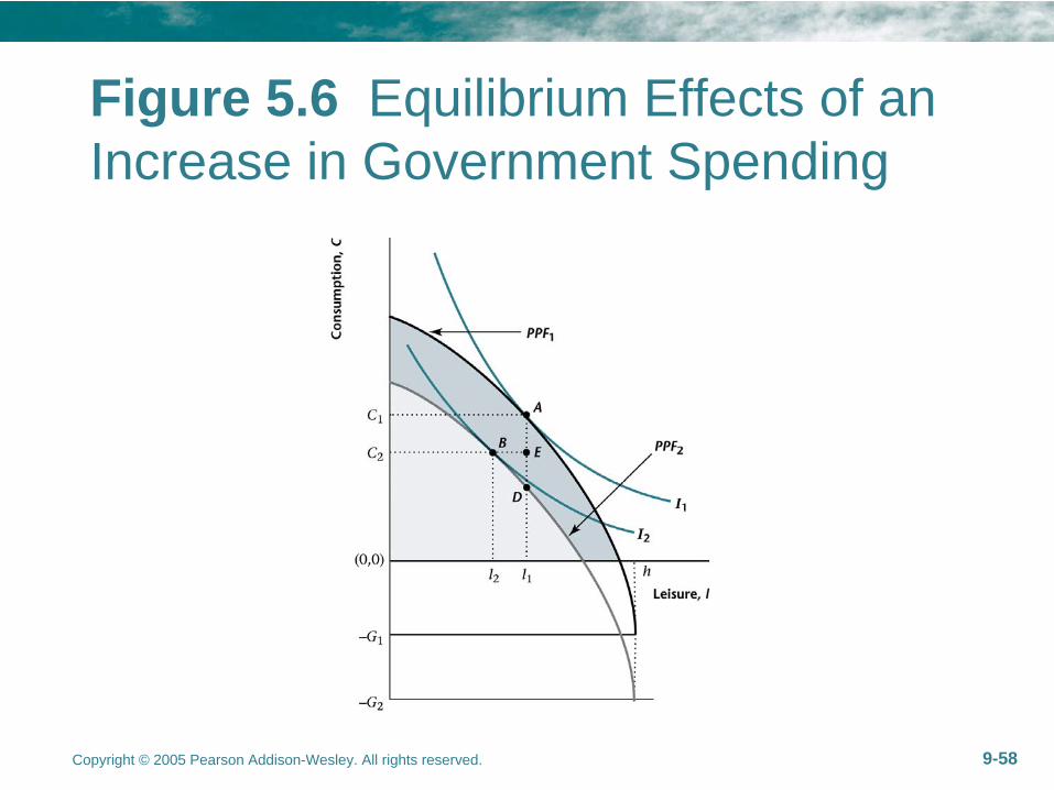
Figure 5.6 Equilibrium Effects of an Increase in Government Spending

Copyright © 2005 Pearson Addison-Wesley. All rights reserved. 9-59
A Permanent Increase in Government Purchases
•
Impact Effects–
Labor Supply: lifetime wealth decreases
labor supply curve shifts to the right–
Output demand: the increase due to G
exactly offset the decrease in demand due to the permanent decrease in lifetime income. There is no change on the output demand curve.
–
Another possibility is the increase in output demand curve is exactly offsetting the supply curve to leave r unchanged.

Copyright © 2005 Pearson Addison-Wesley. All rights reserved. 9-60
•
Equilibrium Effects–
Goods Market: Y,r
–
Labor Market: w, N–
C? (r
makes C, but it might be counted
by the decrease in life time wealth), I (since real interest rate decreases).
Increases in G does not crowd outdoes not crowd out both the consumption and investment.

Copyright © 2005 Pearson Addison-Wesley. All rights reserved. 9-61
Figure 9.20 A Permanent Increase in Government Purchases
Copyright © 2005 Pearson Addison-Wesley. All rights reserved. 9-62
Test the Theory: WWII
•
G•
Previously we knew during this period Y
and C
•
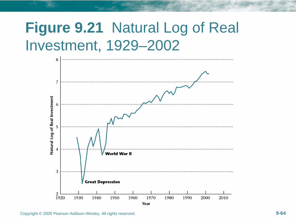
We can also see I•
But real interest rate r was quite low, no increase, contradict to the theory.
Copyright © 2005 Pearson Addison-Wesley. All rights reserved. 9-63
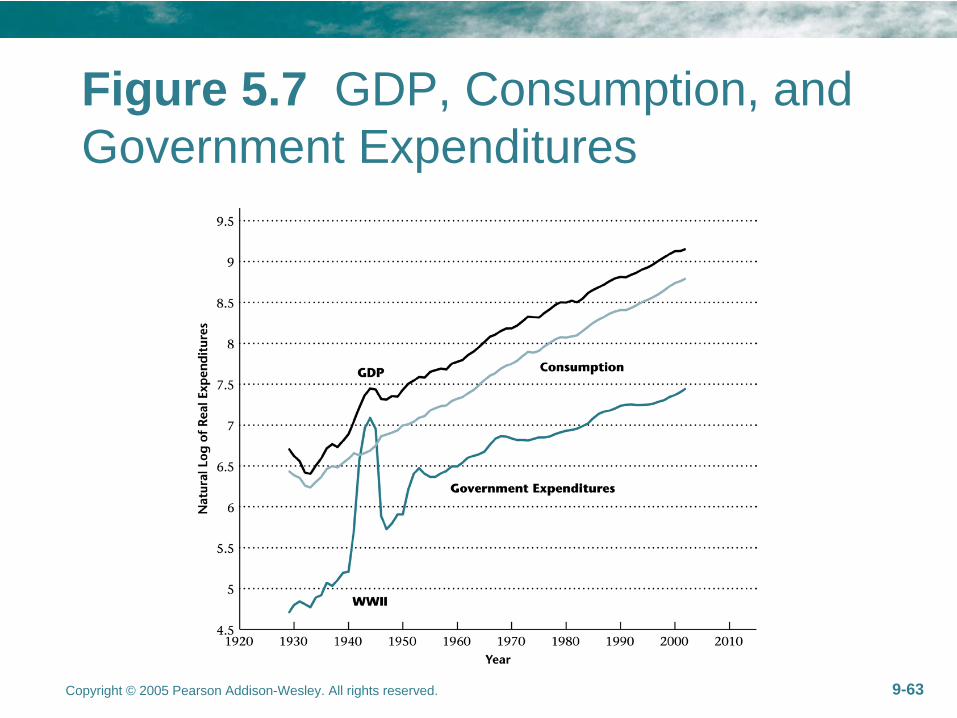
Figure 5.7 GDP, Consumption, and Government Expenditures
Copyright © 2005 Pearson Addison-Wesley. All rights reserved. 9-64
Figure 9.21 Natural Log of Real Investment, 1929–2002
Copyright © 2005 Pearson Addison-Wesley. All rights reserved. 9-65
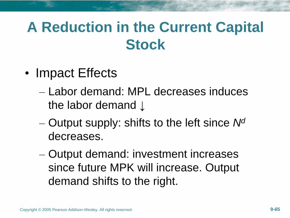
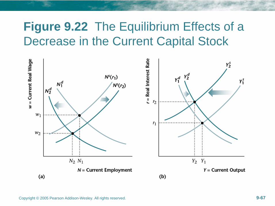
A Reduction in the Current Capital Stock
•
Impact Effects–
Labor demand: MPL decreases induces the labor demand ↓
–
Output supply: shifts to the left since Nd
decreases.–
Output demand: investment increases since future MPK will increase. Output demand shifts to the right.
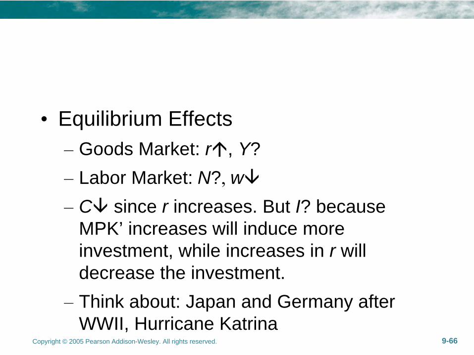
Copyright © 2005 Pearson Addison-Wesley. All rights reserved. 9-66
•
Equilibrium Effects–
Goods Market: r, Y?
–
Labor Market: N?, w–
C
since r increases. But I? because
MPK’ increases will induce more investment, while increases in r will decrease the investment.
–
Think about: Japan and Germany after WWII, Hurricane Katrina
Copyright © 2005 Pearson Addison-Wesley. All rights reserved. 9-67
Figure 9.22 The Equilibrium Effects of a Decrease in the Current Capital Stock

Copyright © 2005 Pearson Addison-Wesley. All rights reserved. 9-68
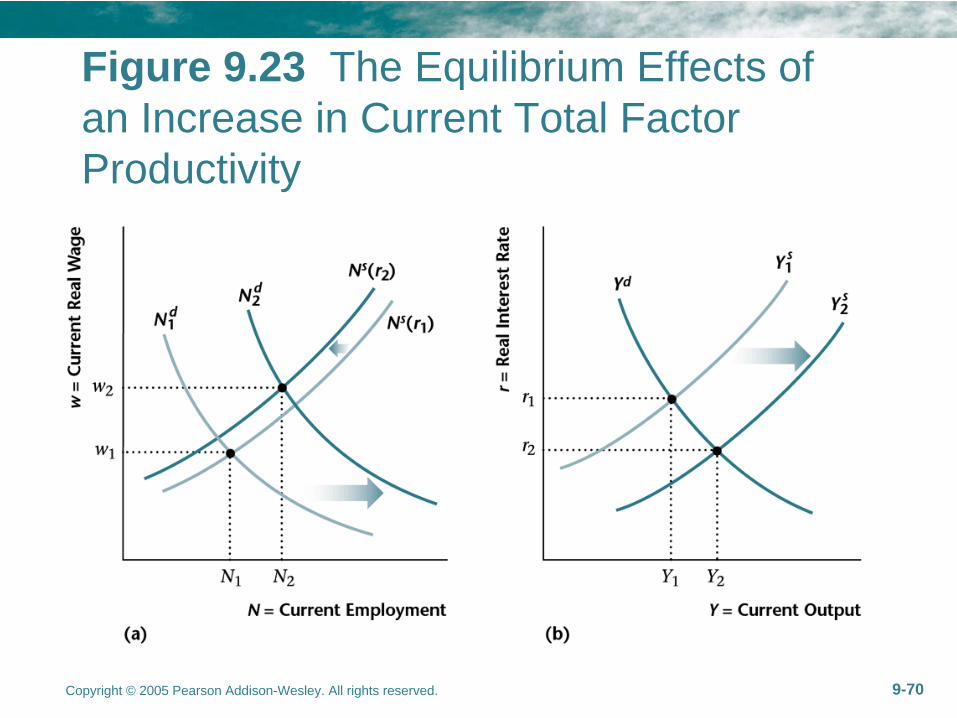
An Increase in Current TFP
•
Impact Effects–
Labor demand: MPL increases, shifts the curve to the right
–
Output supply: shifts to the right

Copyright © 2005 Pearson Addison-Wesley. All rights reserved. 9-69
•
General equilibrium effect–
Goods market: Y, r
–
Labor market: w, N? (likely increase)–
C
(both Y
and r
increase C), I
•
Recall the business cycle facts, the model predicts that consumption, employment (likely), investment, and the real wage are all procyclical, just as in the data.
Copyright © 2005 Pearson Addison-Wesley. All rights reserved. 9-70
Figure 9.23 The Equilibrium Effects of an Increase in Current Total Factor Productivity
Copyright © 2005 Pearson Addison-Wesley. All rights reserved. 9-71
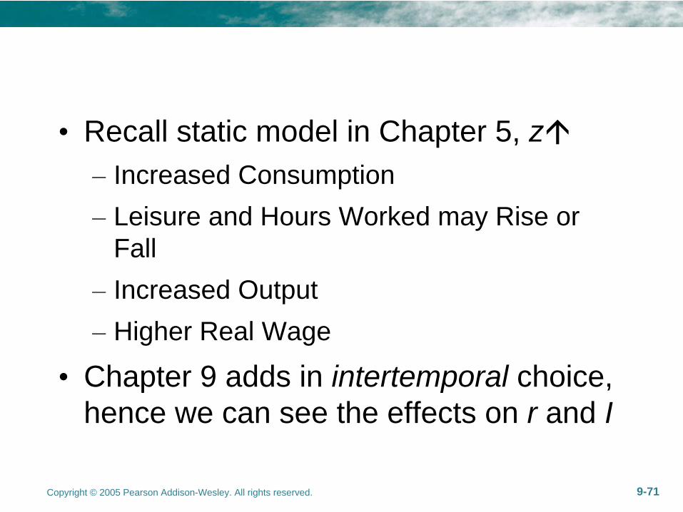
•
Recall static model in Chapter 5, z–
Increased Consumption
–
Leisure and Hours Worked may Rise or Fall
–
Increased Output –
Higher Real Wage
•
Chapter 9 adds in intertemporal choice, hence we can see the effects on r and I

Copyright © 2005 Pearson Addison-Wesley. All rights reserved. 9-72
Figure 5.9 Competitive Equilibrium Effects of an Increase in Total Factor Productivity

Copyright © 2005 Pearson Addison-Wesley. All rights reserved. 9-73
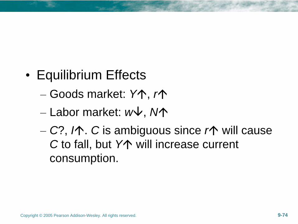
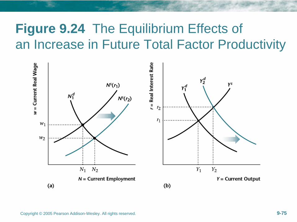
An Increase in Future TFP
•
Impact Effects–
Output demand: z’
will increase MPK’, so
firm wants to invest more–
Labor supply: r
will make it shift to the
right
Copyright © 2005 Pearson Addison-Wesley. All rights reserved. 9-74
•
Equilibrium Effects–
Goods market: Y, r
–
Labor market: w, N–
C?, I. C is ambiguous since r
will cause
C to fall, but Y
will increase current consumption.
Copyright © 2005 Pearson Addison-Wesley. All rights reserved. 9-75
Figure 9.24 The Equilibrium Effects of an Increase in Future Total Factor Productivity

Copyright © 2005 Pearson Addison-Wesley. All rights reserved. 9-76
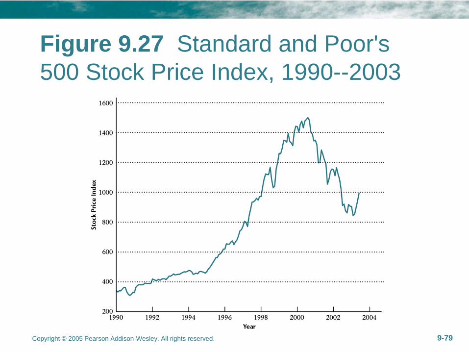
The “New Economy” and Stock Market Bust
•
Increasing optimism about future TFP leads to increases in I and Y, is also reflected in increases in stock prices.
•
Increasing pessimism exactly does the opposite.
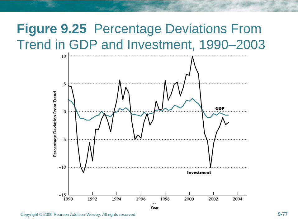
Copyright © 2005 Pearson Addison-Wesley. All rights reserved. 9-77
Figure 9.25 Percentage Deviations From Trend in GDP and Investment, 1990–2003

Copyright © 2005 Pearson Addison-Wesley. All rights reserved. 9-78
Figure 9.26 Investment as a Percentage of GDP, 1990--2003
Copyright © 2005 Pearson Addison-Wesley. All rights reserved. 9-79
Figure 9.27 Standard and Poor's 500 Stock Price Index, 1990--2003

Copyright © 2005 Pearson Addison-Wesley. All rights reserved. 9-80
Sectoral Shocks
•
A sectoral shock is a shift in production from one sector of the economy to another, caused by a shift in demand or a change in relative productivities between sectors.
•
Impact effect: Labor supply curve will shift to the left due to the temporary dislocation of labor from the declining sector. But there is no effect on the aggregate demand for the consumption and investment.

Copyright © 2005 Pearson Addison-Wesley. All rights reserved. 9-81
•
General equilibrium effect–
Goods market: Y, r
–
Labor market: w, N–
The shock is temporary. Once the workers are reallocated, the economy returns to its initial equilibrium.
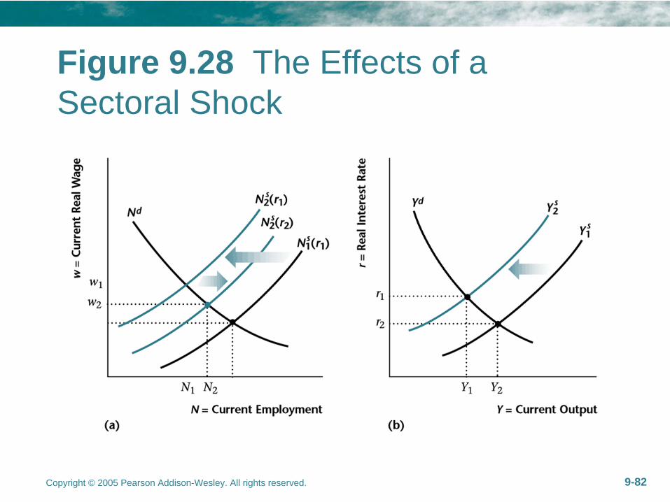
Copyright © 2005 Pearson Addison-Wesley. All rights reserved. 9-82
Figure 9.28 The Effects of a Sectoral Shock

Copyright © 2005 Pearson Addison-Wesley. All rights reserved. 9-83
Discussion
•
What is the macro effect of the failure of GM?

Copyright © 2005 Pearson Addison-Wesley. All rights reserved. 9-84
Figure 9.29 Percentage Deviations From Trend in GDP and Employment, 1990–2003


