Speech Communication 43 (2004) 311–329

www.elsevier.com/locate/specom

A real-time music-scene-description system:predominant-F0 estimation for detecting melody and bass

lines in real-world audio signals q

Masataka Goto *

National Institute of Advanced Industrial Science and Technology (AIST), 1-1-1 Umezono, Tsukuba, Ibaraki 305-8568, Japan

Received 22 May 2002; received in revised form 9 May 2003; accepted 13 March 2004

Abstract

In this paper, we describe the concept of music scene description and address the problem of detecting melody and

bass lines in real-world audio signals containing the sounds of various instruments. Most previous pitch-estimation

methods have had difficulty dealing with such complex music signals because these methods were designed to deal with

mixtures of only a few sounds. To enable estimation of the fundamental frequency (F0) of the melody and bass lines, we

propose a predominant-F0 estimation method called PreFEst that does not rely on the unreliable fundamental compo-

nent and obtains the most predominant F0 supported by harmonics within an intentionally limited frequency range.

This method estimates the relative dominance of every possible F0 (represented as a probability density function of

the F0) by using MAP (maximum a posteriori probability) estimation and considers the F0�s temporal continuity by

using a multiple-agent architecture. Experimental results with a set of ten music excerpts from compact-disc recordings

showed that a real-time system implementing this method was able to detect melody and bass lines about 80% of the

time these existed.

� 2004 Elsevier B.V. All rights reserved.

Keywords: F0 estimation; MAP estimation; EM algorithm; Music understanding; Computational auditory scene analysis; Music

information retrieval

0167-6393/$ - see front matter � 2004 Elsevier B.V. All rights reserv

doi:10.1016/j.specom.2004.07.001

q Supported by ‘‘Information and Human Activity’’, Pre-

cursory Research for Embryonic Science and Technology

(PRESTO), Japan Science and Technology Corporation (JST).* Corresponding author. Tel.: +81 29 861 5898; fax: +81 29

861 3313.

E-mail address: m.goto@aist.go.jp

1. Introduction

A typical research approach to computational

auditory scene analysis (CASA) (Bregman, 1990;

Brown, 1992; Cooke and Brown, 1993; Rosenthal

and Okuno, 1995; Okuno and Cooke, 1997;

ed.

1 As known from the scaling-up problem (Kitano, 1993) in

the domain of artificial intelligence, it is hard to scale-up a

system whose preliminary implementation works only in labo-

ratory (toy-world) environments with unrealistic assumptions.

312 M. Goto / Speech Communication 43 (2004) 311–329

Rosenthal and Okuno, 1998) is sound source segre-

gation: the extraction of the audio signal corre-

sponding to each auditory stream in a sound

mixture. Human listeners can obviously under-

stand various properties of the sound mixtures theyhear in a real-world environment and this suggests

that they detect the existence of certain auditory

objects in sound mixtures and obtain a description

of them. This understanding, however, is not neces-

sarily evidence that the human auditory system ex-

tracts the individual audio signal corresponding to

each auditory stream. This is because segregation is

not a necessary condition for understanding: evenif a mixture of two objects cannot be segregated,

that the mixture includes the two objects can be

understood from their salient features. In develop-

ing a computational model of monaural or binau-

ral sound source segregation, we might be dealing

with a problem which is not solved by any mecha-

nism in this world, not even by the human brain,

although sound source segregation is valuable fromthe viewpoint of engineering.

In the context of CASA, we therefore consider

it essential to build a computational model that

can obtain a certain description of the auditory

scene from sound mixtures. To emphasize its dif-

ference from sound source segregation and resto-

ration, we call this approach auditory scene

description. Kashino (1994) discussed the auditoryscene analysis problem from a standpoint similar

to ours by pointing out that the extraction of sym-

bolic representation is more natural and essential

than the restoration of a target signal wave from

a sound mixture; he did not, however, address

the issue of subsymbolic description which we deal

with below.

In modeling the auditory scene description, it isimportant that we discuss what constitutes an

appropriate description of audio signals. An easy

way of specifying the description is to borrow

the terminology of existing discrete symbol sys-

tems, such as musical scores consisting of musical

notes or speech transcriptions consisting of text

characters. Those symbols, however, fail to express

non-symbolic properties such as the expressivenessof a musical performance and the prosody of spon-

taneous speech. To take such properties into ac-

count, we need to introduce a subsymbolic

description represented as continuous quantitative

values. At the same time, we need to choose an

appropriate level of abstraction for the descrip-

tion, because even though descriptions such as

raw waveforms and spectra have continuous val-ues they are too concrete. The appropriateness of

the abstraction level will depend, of course, on

the purpose of the description and on the use to

which it will be put.

The focus of this paper is on the problem of

music scene description––that is, auditory scene

description in music––for monaural complex

real-world audio signals such as those recordedon commercially distributed compact discs. The

audio signals are thus assumed to contain simul-

taneous sounds of various instruments. This

real-world-oriented approach with realistic assum-

ptions is important to address the scaling-up prob-

lem 1 and facilitate the implementation of practical

applications (Goto and Muraoka, 1996, 1998;

Goto, 2001).The main contribution of this paper is to pro-

pose a predominant-F0 estimation method that

makes it possible to detect the melody and bass

lines in such audio signals. On the basis of this

method, a real-time system estimating the funda-

mental frequencies (F0s) of these lines has been

implemented as a subsystem of our music-scene-

description system. In the following sections, wediscuss the description used in the music-scene-

description system and the difficulties encountered

in detecting the melody and bass lines. We then de-

scribe the algorithm of the predominant-F0 esti-

mation method that is a core part of our system.

Finally, we show experimental results obtained

using our system.

2. Music-scene-description problem

Here, we explain the entire music-scene-descrip-

tion problem. We also explain the main difficulties

Hierarchicalbeat structure

Chord changepossibility

Drum pattern

Melody line

Bass line

Bassdrum

Snaredrum

Musicalaudio signals

time

Fig. 1. Description in our music-scene-description system.

2 Although the basic concept of music scene description is

independent of music genres, some subsymbolic representations

in Fig. 1 depend on genres in our current implementation. The

hierarchical beat structure, chord change possibility, and drum

pattern are obtained under the assumption that an input song is

popular music and its time-signature is 4/4. On the other hand,

the melody and bass lines are obtained for music, in any genre,

having single-tone melody and bass lines.

M. Goto / Speech Communication 43 (2004) 311–329 313

in detecting the melody and bass lines––the sub-

problem that we deal with in this paper.

2.1. Problem specification

Music scene description is defined as a process

that obtains a description representing the inputmusical audio signal. Since various levels of

description are possible, we must decide which

level is an appropriate first step toward the ulti-

mate description in human brains. We think that

the music score is inadequate for this because, as

pointed out (Goto and Muraoka, 1999), an un-

trained listener understands music to some extent

without mentally representing audio signals asmusical scores. Music transcription, identifying

the names (symbols) of musical notes and chords,

is in fact a skill mastered only by trained musi-

cians. We think that an appropriate description

should be:

• An intuitive description that can be easily

obtained by untrained listeners.• A basic description that trained musicians

can use as a basis for higher-level music

understanding.

• A useful description facilitating the develop-

ment of various practical applications.

According to these requirements, we propose a

description (Fig. 1) consisting of five subsymbolicrepresentations:

(1) Hierarchical beat structure

Represents the fundamental temporal struc-

ture of music and comprises the quarter-note

and measure levels––i.e., the positions of

quarter-note beats and bar-lines.

(2) Chord change possibility

Represents the possibilities of chord changes

and indicates how much change there is in

the dominant frequency components included

in chord tones and their harmonic overtones.

(3) Drum pattern

Represents temporal patterns of how two

principal drums, a bass drum and a snare

drum, are played. This representation is notused for music without drums.

(4) Melody line

Represents the temporal trajectory of the mel-

ody, which is a series of single tones and is

heard more distinctly than the rest. Note that

this is not a series of musical notes; it is a con-tinuous representation of frequency and

power transitions.

(5) Bass line

Represents the temporal trajectory of the

bass, which is a series of single tones and is

the lowest part in polyphonic music. This is

a continuous representation of frequency

and power transitions.

The idea behind these representations came

from introspective observation of how untrained

listeners listen to music. A description consisting

of the first three representations and the methods

for obtaining them were described previously

(Goto and Muraoka, 1994, 1996, 1998, 1999;

Goto, 1998, 2001) from the viewpoint of beattracking. 2

In this paper we deal with the last two represen-

tations, the melody line and bass line. The detection

314 M. Goto / Speech Communication 43 (2004) 311–329

of the melody and bass lines is important because

the melody forms the core of Western music and

is very influential in the identity of a musical piece

and the bass is closely related to the tonality. These

lines are fundamental to the perception of music byboth trained and untrained listeners. They are also

useful in various applications such as automatic

transcription, automatic music indexing for infor-

mation retrieval (e.g., searching for a song by sin-

ging a melody), computer participation in live

human performances, musical performance analysis

of outstanding recorded performances, and auto-

matic production of accompaniment tracks forKaraoke or Music Minus One using compact discs.

In short, we solve the problem of obtaining a

description of the melody line Sm(t) and the bass

line Sb(t) given by

SmðtÞ ¼ fF mðtÞ;AmðtÞg; ð1Þ

SbðtÞ ¼ fF bðtÞ;AbðtÞg; ð2Þ

where Fi(t) (i = m,b) denotes the fundamental fre-

quency (F0) at time t and Ai(t) denotes the power

at t.

2.2. Problems in detecting the melody and bass lines

It has been considered difficult to estimate the

F0 of a particular instrument or voice in the mon-

aural audio signal of an ensemble performed by

more than three musical instruments. Most previ-

ous F0 estimation methods (Noll, 1967; Schroeder,

1968; Rabiner et al., 1976; Nehorai and Porat,

1986; Charpentier, 1986; Ohmura, 1994; Abe

et al., 1996; Kawahara et al., 1999) have beenpremised upon the input audio signal containing

just a single-pitch sound with aperiodic noise.

Although several methods for dealing with multi-

ple-pitch mixtures have been proposed (Parsons,

1976; Chafe and Jaffe, 1986; Katayose and Inoku-

chi, 1989; de Cheveigne, 1993; Brown and Cooke,

1994; Nakatani et al., 1995; Kashino and Murase,

1997; Kashino et al., 1998; de Cheveigne andKawahara, 1999; Tolonen and Karjalainen, 2000;

Klapuri, 2001), these required that the number of

simultaneous sounds be assumed and had diffi-

culty estimating the F0 in complex audio signals

sampled from compact discs.

The main reason F0 estimation in sound mix-

tures is difficult is that in the time–frequency do-

main the frequency components of one sound

often overlap the frequency components of simul-

taneous sounds. In popular music, for example,part of the voice�s harmonic structure is often

overlapped by harmonics of the keyboard instru-

ment or guitar, by higher harmonics of the bass

guitar, and by noisy inharmonic frequency compo-

nents of the snare drum. A simple method of

locally tracing a frequency component is therefore

neither reliable nor stable. Moreover, sophis-

ticated F0 estimation methods relying on the ex-istence of the F0�s frequency component (the

frequency component corresponding to the F0)

not only cannot handle the missing fundamental,

but are also unreliable when the F0�s frequency

component is smeared by the harmonics of simul-

taneous sounds.

Taking the above into account, the main prob-

lems in detecting the melody and bass lines can besummarized as:

(i) How to decide which F0 belongs to the mel-

ody and bass lines in polyphonic music.

(ii) How to estimate the F0 in complex sound

mixtures where the number of sound sources

is unknown.

(iii) How to select the appropriate F0 when sev-eral ambiguous F0 candidates are found.

3. Predominant-F0 estimation method: PreFEst

We propose a method called PreFEst (predom-

inant-F0 estimation method) which makes it possi-

ble to detect the melody and bass lines in

real-world sound mixtures. In solving the above

problems, we make three assumptions:

• The melody and bass sounds have a harmonic

structure. However, we do not care about the

existence of the F0�s frequency component.

• The melody line has the most predominant

(strongest) harmonic structure in middle- and

high-frequency regions and the bass line has

the most predominant harmonic structure in alow-frequency region.

Limiting frequency regions

Interaction Agent

AgentAgent

Detecting m

elody

Detecting bass lin

Audio signals

Instantaneous frequency calculation

Salience detector

BPF for melody line BPF for bass line

Forming F0's probability density function

F0's probability density function

Extracting frequency components

Frequency components

PreF

Est-fro

nt-en

dP

reFE

st-core

PreF

Est-b

acM. Goto / Speech Communication 43 (2004) 311–329 315

• The melody and bass lines tend to have tempo-

rally continuous trajectories: the F0 is likely to

continue at close to the previous F0 for its dura-

tion (i.e., during a musical note).

These assumptions fit a large class of music with

single-tone melody and bass lines.

PreFEst basically estimates the F0 of the most

predominant harmonic structure within a limited

frequency range of a sound mixture. Our solutions

to the three problems mentioned above are out-

lined as follows: 3

(i) The method intentionally limits the frequency

range to middle- and high-frequency regions

for the melody line and to a low frequency

region for the bass line, and finds the F0

whose harmonics are most predominant in

those ranges. In other words, whether the

F0 is within the limited range or not, PreFEst

tries to estimate the F0 which is supported bypredominant harmonic frequency compo-

nents within that range.

(ii) The method regards the observed frequency

components as a weighted mixture of all pos-

sible harmonic-structure tone models without

assuming the number of sound sources. It

estimates their weights by using the Expecta-

tion-Maximization (EM) algorithm (Demp-ster et al., 1977), which is an iterative

technique for computing maximum likelihood

estimates and MAP (maximum a posteriori

probability) estimates from incomplete data.

The method then considers the maximum-

weight model as the most predominant har-

monic structure and obtains its F0. Since the

above processing does not rely on the exist-ence of the F0�s frequency component, it can

deal with the missing fundamental.

(iii) Because multiple F0 candidates are found in

an ambiguous situation, the method considers

their temporal continuity and selects the most

3 In this paper, we do not deal with the problem of detecting

the absence (activity) of melody and bass lines. PreFEst simply

estimates the predominant F0 without discriminating between

the sound sources.

dominant and stable trajectory of the F0 as

the output. For this sequential F0 tracking,

we introduce a multiple-agent architecture in

which agents track different temporal trajec-

tories of the F0.

While we do not intend to build a psychoacous-

tical model of human perception, certain psycho-

acoustical results may have some relevance

concerning our strategy: Ritsma (1967) reported

that the ear uses a rather limited spectral region

in achieving a well-defined pitch perception;

Plomp (1967) concluded that for fundamental fre-quencies up to about 1400 Hz, the pitch of a com-

plex tone is determined by the second and higher

harmonics rather than by the fundamental. Note,

however, that those results do not directly support

our strategy since they were obtained by using the

pitch of a single sound.

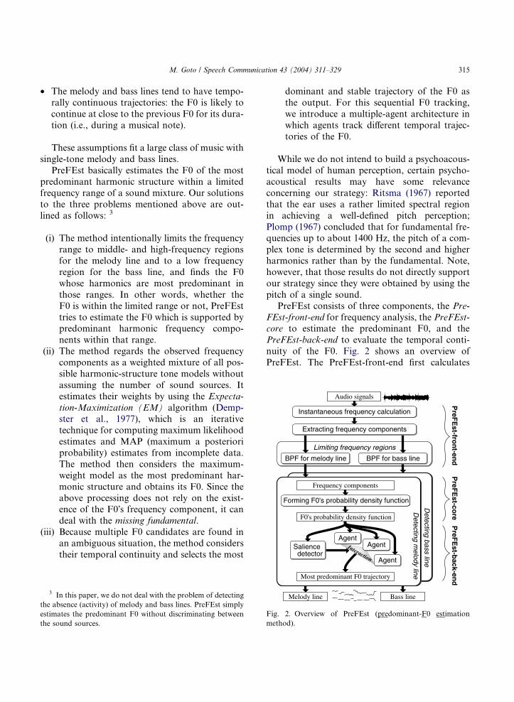
PreFEst consists of three components, the Pre-

FEst-front-end for frequency analysis, the PreFEst-core to estimate the predominant F0, and the

PreFEst-back-end to evaluate the temporal conti-

nuity of the F0. Fig. 2 shows an overview of

PreFEst. The PreFEst-front-end first calculates

line

e

Melody line Bass line

Most predominant F0 trajectory

k-end

Fig. 2. Overview of PreFEst (predominant-F0 estimation

method).

316 M. Goto / Speech Communication 43 (2004) 311–329

instantaneous frequencies by using multirate signal

processing techniques and extracts frequency com-

ponents on the basis of an instantaneous-fre-

quency-related measure. By using two bandpass

filters (BPFs), it limits the frequency range of thesecomponents to middle and high regions for the

melody line and to a low region for the bass line.

The PreFEst-core then forms a probability density

function (PDF) for the F0 which represents the rel-

ative dominance of every possible harmonic struc-

ture. To form the F0�s PDF, it regards each set of

filtered frequency components as a weighted mix-

ture of all possible harmonic-structure tone modelsand then estimates their weights which can be

interpreted as the F0�s PDF; the maximum-weight

model corresponds to the most predominant har-

monic structure. This estimation is carried out

using MAP estimation and the EM algorithm. Fi-

nally, in the PreFEst-back-end, multiple agents

track the temporal trajectories of promising salient

peaks in the F0�s PDF and the output F0 is deter-mined on the basis of the most dominant and sta-

ble trajectory.

3.1. PreFEst-front-end: forming the observed prob-

ability density functions

The PreFEst-front-end uses a multirate filter

bank to obtain adequate time and frequency reso-lution and extracts frequency components by using

an instantaneous-frequency-related measure. It

obtains two sets of bandpass-filtered frequency

components, one for the melody line and the other

for the bass line.

3.1.1. Instantaneous frequency calculation

The PreFEst-front-end first calculates theinstantaneous frequency (Flanagan and Golden,

1966; Boashash, 1992), the rate of change of the

= LPF (0.45 fs) + 1/2 down-sampler

Decimator16 kHz

8 kHz

4 kHz2 DecimatorDecim

Decimator

Audio signals

Fig. 3. Structure of the m

signal phase, of filter-bank outputs. It uses an effi-

cient calculation method (Flanagan and Golden,

1966) based on the short-time Fourier transform

(STFT) whose output can be interpreted as a col-

lection of uniform-filter outputs. When the STFTof a signal x(t) with a window function h(t) is de-

fined as

X ðx; tÞ ¼Z 1

�1xðsÞhðs � tÞe�jxsds ð3Þ

¼ aþ jb; ð4Þ

the instantaneous frequency k(x, t) is given by

kðx; tÞ ¼ x þa ob

ot � b oaot

a2 þ b2: ð5Þ

To obtain adequate time–frequency resolution

under the real-time constraint, we designed an

STFT-based multirate filter bank (Fig. 3). At each

level of the binary branches, the audio signal isdown-sampled by a decimator that consists of an

anti-aliasing filter (an FIR lowpass filter (LPF))

and a 1/2 down-sampler. The cut-off frequency of

the LPF in each decimator is 0.45 fs, where fs is

the sampling rate at that branch. In our current

implementation, the input signal is digitized at 16

bit/16 kHz and is finally down-sampled to 1 kHz.

Then the STFT, whose window size is 512 samples,is calculated at each leaf by using the Fast Fourier

Transform (FFT) while compensating for the time

delays of the different multirate layers. Since at 16

kHz the FFT frame is shifted by 160 samples, the

discrete time step (1 frame-time) is 10 ms. This

paper uses time t for the time measured in units

of frame-time.

3.1.2. Extracting frequency components

The extraction of frequency components is

based on the mapping from the center frequency

x of an STFT filter to the instantaneous frequency

FFT

FFTFFTFFTFFT

2 kHz1kHz

atorDecimator

0-0.45kHz

0.45-0.9kHz

0.9-1.8kHz

1.8-3.6kHz

3.6-7.2kHz

ultirate filter bank.

M. Goto / Speech Communication 43 (2004) 311–329 317

k(x, t) of its output (Charpentier, 1986; Abe et al.,

1996; Kawahara et al., 1999). If there is a fre-

quency component at frequency w, that frequency

is placed at the fixed point of the mapping and

the instantaneous frequencies around w stayalmost constant in the mapping (Kawahara et al.,

1999). Therefore, a set WðtÞf of instantaneous fre-

quencies of the frequency components can be

extracted by using the equation (Abe et al., 1997)

WðtÞf ¼ w j kðw; tÞ � w ¼ 0;

o

owðkðw; tÞ � wÞ < 0

� �:

ð6ÞBy calculating the power of those frequencies,which is given by the STFT spectrum at WðtÞ

f , we

can define the power distribution function

WðtÞp ðxÞ as

WðtÞp ðxÞ ¼ j X ðx; tÞ j if x 2 WðtÞ

f ;

0 otherwise:

(ð7Þ

3.1.3. Limiting frequency regions

The frequency range is intentionally limited by

using the two BPFs whose frequency responses

are shown in Fig. 4. The BPF for the melody line

is designed so that it covers most of the dominantharmonics of typical melody lines and deempha-

sizes the crowded frequency region around the

F0: it does not matter if the F0 is not within the

passband. The BPF for the bass line is designed

so that it covers most of the dominant harmonics

of typical bass lines and deemphasizes a frequency

region where other parts tend to become more

dominant than the bass line.The filtered frequency components can be

represented as BPF iðxÞW0ðtÞp ðxÞ, where BPFi(x)

(i = m,b) is the BPF�s frequency response for the

melody line (i = m) and the bass line (i = b), and

BPF for detecting bass line

1200 cent 2400 cent 3600 cent 4800 cent0 cent

16.35Hz 32.70 Hz 65.41 Hz 130.8 Hz 261.6 Hz

1

Fig. 4. Frequency responses of

x is the log-scale frequency denoted in units of

cents (a musical-interval measurement). Frequency

fHz in Hertz is converted to frequency fcent in cents

as follows:

fcent ¼ 1200log2

fHz

440 � 2312�5

: ð8Þ

There are 100 cents to a tempered semitone and

1200 to an octave. The power distributionW0ðtÞ

p ðxÞ is the same as WðtÞp ðxÞ except that the fre-

quency unit is the cent.

To enable the application of statistical methods,

we represent each of the bandpass-filtered fre-

quency components as a probability density func-

tion (PDF), called an observed PDF, pðtÞW ðxÞ:

pðtÞW ðxÞ ¼BPF iðxÞW0ðtÞ

p ðxÞR1�1 BPF iðxÞW0ðtÞ

p ðxÞdx: ð9Þ

3.2. PreFEst-core: estimating the F0�s probability

density function

For each set of filtered frequency components

represented as an observed PDF pðtÞW ðxÞ, the Pre-

FEst-core forms a probability density function of

the F0, called the F0�s PDF, pðtÞF0ðF Þ, where F is

the log-scale frequency in cents. We consider each

observed PDF to have been generated from a

weighted-mixture model of the tone models of all

the possible F0s; a tone model is the PDF corre-sponding to a typical harmonic structure and indi-

cates where the harmonics of the F0 tend to occur.

Because the weights of tone models represent the

relative dominance of every possible harmonic

structure, we can regard these weights as the F0�sPDF: the more dominant a tone model is in the

mixture, the higher the probability of the F0 of

its model.

BPF for detecting melody line

6000 cent 7200 cent 8400 cent 9600 cent

523.3 Hz 1047 Hz 2093 Hz 4186 Hz

bandpass filters (BPFs).

Table 1

List of symbols

Symbol Description

t Time

x Log-scale frequency in cents

i The melody line (i = m) or the bass line (i = b)

pðtÞW ðxÞ Observed PDF (bandpass-filtered frequency components) (Eq. (9))

F Fundamental frequency (F0) in cents

p(xjF,m,l(t)(F,m)) PDF of the mth tone model for each F0 F (Eq. (10))

l(t)(F,m) Shape of tone model (l(t)(F,m) = {c(t)(hjF,m)}) (Eq. (12))

c(t)(hjF,m) Relative amplitude of the hth harmonic component (shape of tone model)

Mi The number of tone models

Hi The number of harmonic components for tone model

Wi Standard deviation of the Gaussian distribution for harmonic components

p(xjh(t)) Weighted-mixture model (weighted mixture of tone models) (Eq. (15))

h(t) Model parameter of p(xjh(t)) (Eq. (16))

w(t)(F,m) Weight of tone model p(xjF,m,l(t)(F,m))

Fli, Fhi Lower and upper limits of the possible (allowable) F0 range

pðtÞF0ðF Þ F0�s PDF (Eq. (20))

p0i(h(t)) Prior distribution of the model parameter h(t) (Eq. (21))

p0i(w(t)) Prior distribution of the weight of tone model (Eq. (22))

p0i(l(t)) Prior distribution of the tone-model shapes (Eq. (23))

wðtÞ0i ðF ;mÞ Most probable parameter of w(t)(F,m) (for p0i(w

(t)))

lðtÞ0i ðF ;mÞ ðc

ðtÞ0i ðh j F ;mÞÞ Most probable parameter of l(t)(F,m) (for p0i(l

(t)))

bðtÞwi Parameter determining how much emphasis is put on wðtÞ

0i

bðtÞli ðF ;mÞ Parameter determining how much emphasis is put on lðtÞ

0i ðF ;mÞh0(t) = {w 0(t),l 0(t)} Old parameter estimate for each iteration of the EM algorithm

hðtÞ ¼ fwðtÞ;lðtÞg New parameter estimate for each iteration of the EM algorithm

318 M. Goto / Speech Communication 43 (2004) 311–329

The main symbols used in this section are listed

in Table 1.

3.2.1. Weighted mixture of adaptive tone models

To deal with diversity of the harmonic struc-

ture, the PreFEst-core can use several types of

harmonic-structure tone models. The PDF of

the mth tone model for each F0 F is denoted byp(x jF, m, l(t)(F,m)) (Fig. 5), where the model

parameter l(t)(F,m) represents the shape of the

tone model. The number of tone models is Mi

x [cent]

x [cent]F

c(t)(1|F,1)

c(t)(1|F,2)

c(t)(2|F,1)

c(t)(3|F,1)

c(t)(4|F,1)

c(t)(2|F,2) c(t)(3|F,2)

c(t)(4|F,2)

F+1200

F+2400F+1902

fundamentalfrequency

p(x | F,1,µ(t)(F,1))

p(x | F,2,µ(t)(F,2))(m=2)Tone Model

(m=1)Tone Model

p(x,1 | F,2,µ(t)(F,2))

Fig. 5. Model parameters of multiple adaptive tone models.

(1 6 m 6 Mi) where i denotes the melody line

(i = m) or the bass line (i = b). Each tone model

is defined by

pðx j F ;m; lðtÞðF ;mÞÞ ¼XHi

h¼1

p

ðx; h j F ;m; lðtÞðF ;mÞÞ; ð10Þ

pðx; h j F ;m; lðtÞðF ;mÞÞ ¼ cðtÞðh j F ;mÞGðx; Fþ 1200log2h;WiÞ; ð11Þ

lðtÞðF ;mÞ ¼ fcðtÞðh j F ;mÞ j h ¼ 1; . . . ;Hig; ð12Þ

Gðx; x0; rÞ ¼1ffiffiffiffiffiffiffiffiffiffi

2pr2p exp �ðx� x0Þ2

2r2

" #; ð13Þ

where Hi is the number of harmonics considered,

Wi is the standard deviation r of the Gaussian dis-

tribution G(x;x0,r), and c(t)(hjF,m) determines the

relative amplitude of the hth harmonic component(the shape of the tone model) and satisfies

M. Goto / Speech Communication 43 (2004) 311–329 319

XHi

h¼1

cðtÞðh j F ;mÞ ¼ 1: ð14Þ

In short, this tone model places a weighted

Gaussian distribution at the position of each har-

monic component. 4

We then consider the observed PDF pðtÞW ðxÞ to

have been generated from the following model

p(xjh(t)), which is a weighted mixture of all possible

tone models p(xjF,m,l(t)(F,m)):

pðx j hðtÞÞ ¼Z Fhi

Fli

XMi

m¼1

wðtÞðF ;mÞ

� pðx j F ;m; lðtÞðF ;mÞÞdF ; ð15Þ

hðtÞ ¼ fwðtÞ; lðtÞg; ð16Þ

wðtÞ ¼ fwðtÞðF ;mÞ j Fli 6 F 6 Fhi;

m ¼ 1; . . . ;Mig; ð17Þ

lðtÞ ¼ flðtÞðF ;mÞ j Fli 6 F 6 Fhi;

m ¼ 1; . . . ;Mig; ð18Þ

where Fli and Fhi denote the lower and upper lim-

its of the possible (allowable) F0 range and

w(t)(F,m) is the weight of a tone model

p(xjF,m,l(t)(F,m)) that satisfiesZ Fhi

Fli

XMi

m¼1

wðtÞðF ;mÞdF ¼ 1: ð19Þ

Because we cannot know a priori the number of

sound sources in real-world audio signals, it is

important that we simultaneously take into con-

sideration all F0 possibilities as expressed in Eq.

(15). If we can estimate the model parameter h(t)

such that the observed PDF pðtÞW ðxÞ is likely to have

been generated from the model p(xjh(t)), the weightw(t)(F,m) can be interpreted as the F0�s PDF

pðtÞF0ðF Þ:

pðtÞF0ðF Þ ¼XMi

m¼1

wðtÞðF ;mÞ ðFli 6 F 6 FhiÞ: ð20Þ

4 Although we deal with only harmonic-structure tone

models in this paper, we can also support inharmonic-structure

tone models as discussed later.

3.2.2. Introducing a prior distribution

To use prior knowledge about F0 estimates and

the tone-model shapes, we define a prior distribu-

tion p0i(h(t)) of h(t) as follows:

p0iðhðtÞÞ ¼ p0iðwðtÞÞp0iðlðtÞÞ; ð21Þ

p0iðwðtÞÞ ¼ 1

Zwexp �bðtÞ

wiDwðwðtÞ0i ;w

ðtÞÞh i

; ð22Þ

p0iðlðtÞÞ ¼ 1

Zlexp �

Z Fhi

Fli

XMi

m¼1

bðtÞli ðF ;mÞ

"

�DlðlðtÞ0i ðF ;mÞ; lðtÞðF ;mÞÞdF

#: ð23Þ

Here p0i(w(t)) and p0i(l

(t)) are unimodal distribu-

tions: p0i(w(t)) takes its maximum value at

wðtÞ0i ðF ;mÞ and p0i(l

(t)) takes its maximum value

at lðtÞ0i ðF ;mÞ, where wðtÞ

0i ðF ;mÞ and lðtÞ0i ðF ;mÞ

ðcðtÞ0i ðh j F ;mÞÞ are the most probable parameters.Zw and Zl are normalization factors, and bðtÞ

wi

and bðtÞli ðF ;mÞ are parameters determining how

much emphasis is put on the maximum value.

The prior distribution is not informative (i.e., it

is uniform) when bðtÞwi and bðtÞ

li ðF ;mÞ are 0, corre-

sponding to the case when no prior knowledge is

available. In Eqs. (22) and (23), DwðwðtÞ0i ;w

ðtÞÞ and

DlðlðtÞ0i ðF ;mÞ; lðtÞðF ;mÞÞ are the following Kull-

back–Leibler information: 5

DwðwðtÞ0i ;w

ðtÞÞ ¼Z Fhi

Fli

XMi

m¼1

wðtÞ0i ðF ;mÞ

� logwðtÞ

0i ðF ;mÞwðtÞðF ;mÞ dF ; ð24Þ

DlðlðtÞ0i ðF ;mÞ; lðtÞðF ;mÞÞ

¼XHi

h¼1

cðtÞ0i ðh j F ;mÞ logcðtÞ0i ðh j F ;mÞcðtÞðh j F ;mÞ : ð25Þ

DwðwðtÞ0i ;w

ðtÞÞ represents the closeness between wðtÞ0i

and w(t) and DlðlðtÞ0i ðF ;mÞ; lðtÞðF ;mÞÞ represents

the closeness between lðtÞ0i ðF ;mÞ and l(t)(F,m).

5 We use Eqs. (24) and (25) because they are intuitive and

are also convenient in the derivations that follow.

320 M. Goto / Speech Communication 43 (2004) 311–329

3.2.3. MAP estimation using the EM algorithm

The problem to be solved is to estimate the

model parameter h(t), taking into account the prior

distribution p0i(h(t)), when we observe pðtÞW ðxÞ. The

MAP (maximum a posteriori probability) estima-tor of h(t) is obtained by maximizing

Z 1

�1pðtÞW ðxÞðlog pðx j hðtÞÞ þ log p0iðhðtÞÞÞdx: ð26Þ

Because this maximization problem is too diffi-

cult to solve analytically, we use the EM (Expecta-

tion-Maximization) algorithm to estimate h(t).While the EM algorithm is usually used for com-

puting maximum likelihood estimates from incom-

plete observed data, it can also be used for

computing MAP estimates as described in (Demp-

ster et al., 1977). In the maximum likelihood esti-

mation, the EM algorithm iteratively applies two

steps, the expectation step (E-step) to compute

the conditional expectation of the mean log-likeli-hood and the maximization step (M-step) to maxi-

mize its expectation. On the other hand, in the

MAP estimation, the algorithm iteratively applies

the E-step to compute the sum of the conditional

expectation and the log prior distribution and

the M-step to maximize it. With respect to h(t),

each iteration updates the old estimate h 0(t) =

{w 0(t),l 0(t)} to obtain the new (improved) estimate

hðtÞ ¼ fwðtÞ; lðtÞg. For each frame t, w 0(t) is initial-

ized with the final estimate wðt�1Þ after iterations

at the previous frame t � 1; l 0(t) is initialized with

the most probable parameter lðtÞ0i in our current

implementation.

By introducing the hidden (unobservable) vari-

ables F, m, and h, which, respectively, describewhich F0, which tone model, and which harmonic

component were responsible for generating each

observed frequency component at x, we can spec-

ify the two steps as follows:

(1) (E-step)

Compute the following QMAP(h(t)jh 0(t)) for the

MAP estimation:

QMAPðhðtÞ j h0ðtÞÞ ¼ QðhðtÞ j h0ðtÞÞ þ log p0iðhðtÞÞ;ð27Þ

QðhðtÞ j h0ðtÞÞ

¼Z 1

�1pðtÞW ðxÞEF ;m;h½logpðx;F ;m;h j hðtÞÞ j x;h0ðtÞ�dx;

ð28Þ

where Q(h(t)jh 0(t)) is the conditional expectation of

the mean log-likelihood for the maximum likeli-

hood estimation. EF,m,h[ajb] denotes the condi-

tional expectation of a with respect to the hidden

variables F, m, and h with the probability distribu-

tion determined by condition b.

(2) (M-step)Maximize QMAP(h(t)jh 0(t)) as a function of h(t) to

obtain the updated (improved) estimate hðtÞ:

hðtÞ ¼ argmaxhðtÞ

QMAPðhðtÞ j h0ðtÞÞ: ð29Þ

In the E-step, Q(h(t)jh 0(t)) is expressed as

QðhðtÞ j h0ðtÞÞ ¼Z 1

�1

Z Fhi

Fli

XMi

m¼1

XHi

h¼1

pðtÞW ðxÞpðF ;m; h j x; h0ðtÞÞ

� log pðx; F ;m; h j hðtÞÞdF dx; ð30Þ

where the complete-data log-likelihood is given by

log pðx; F ;m; h j hðtÞÞ¼ logðwðtÞðF ;mÞpðx; h j F ;m; lðtÞðF ;mÞÞÞ: ð31Þ

From Eq. (21), the log prior distribution is given

by

logp0iðhðtÞÞ

¼� logZwZl �Z Fhi

Fli

XMi

m¼1

bðtÞwiw

ðtÞ0i ðF ;mÞ log

wðtÞ0i ðF ;mÞ

wðtÞðF ;mÞ

þbðtÞli ðF ;mÞ

XHi

h¼1

cðtÞ0i ðh j F ;mÞ logcðtÞ0i ðh j F ;mÞcðtÞðh j F ;mÞ

!dF :

ð32Þ

Regarding the M-step, Eq. (29) is a conditional

problem of variation, where the conditions are

given by Eqs. (14) and (19). This problem can be

solved by using the following Euler-Lagrange dif-

ferential equations with Lagrange multipliers kwand kl:

M. Goto / Speech Communication 43 (2004) 311–329 321

o

owðtÞ

Z 1

�1

XHi

h¼1

pðtÞW ðxÞpðF ;m;h j x;h0ðtÞÞðlogwðtÞðF ;mÞ

þ logpðx;h j F ;m;lðtÞðF ;mÞÞÞdx

�bðtÞwiw

ðtÞ0i ðF ;mÞ log

wðtÞ0i ðF ;mÞ

wðtÞðF ;mÞ

�kw wðtÞðF ;mÞ� 1

MiðFhi�FliÞ

� �!¼ 0; ð33Þ

o

ocðtÞ

Z 1

�1pðtÞW ðxÞpðF ;m; h j x; h0ðtÞÞ

�ðlogwðtÞðF ;mÞ

þ log cðtÞðh j F ;mÞ þ logGðx; Fþ1200log2h;WiÞÞdx

�bðtÞli ðF ;mÞc

ðtÞ0i ðh j F ;mÞ log

cðtÞ0i ðh j F ;mÞcðtÞðh j F ;mÞ

�kl cðtÞðh j F ;mÞ � 1

Hi

� ��¼ 0: ð34Þ

From these equations we get

wðtÞðF ;mÞ ¼ 1

kw

Z 1

�1pðtÞW ðxÞpðF ;m j x; h0ðtÞÞdx

�

þbðtÞwiw

ðtÞ0i ðF ;mÞ

�; ð35Þ

cðtÞðh j F ;mÞ ¼ 1

kl

Z 1

�1pðtÞW ðxÞpðF ;m; h j x; h0ðtÞÞdx

�

þbðtÞli ðF ;mÞc

ðtÞ0i ðh j F ;mÞ

�: ð36Þ

In these equations, kw and kl are determined from

Eqs. (14) and (19) as

kw ¼ 1 þ bðtÞwi ; ð37Þ

kl ¼Z 1

�1pðtÞW ðxÞpðF ;m j x; h0ðtÞÞdx

þ bðtÞli ðF ;mÞ: ð38Þ

According to Bayes� theorem, p(F,m,hjx,h 0(t)) and

p(F,mjx,h 0(t)) are given by

pðF ;m; h j x; h0ðtÞÞ

¼ w0ðtÞðF ;mÞpðx; h j F ;m; l0ðtÞðF ;mÞÞpðx j h0ðtÞÞ

; ð39Þ

pðF ;m j x; h0ðtÞÞ

¼ w0ðtÞðF ;mÞpðx j F ;m; l0ðtÞðF ;mÞÞpðx j h0ðtÞÞ

: ð40Þ

Finally, we obtain the new parameter estimates

wðtÞðF ; mÞ and cðtÞðhjF ; mÞ:

wðtÞðF ;mÞ ¼ wðtÞMLðF ;mÞ þ bðtÞ

wiwðtÞ0i ðF ;mÞ

1 þ bðtÞwi

; ð41Þ

cðtÞðh j F ;mÞ

¼wðtÞ

MLðF ;mÞcðtÞMLðh j F ;mÞþbðtÞ

li ðF ;mÞcðtÞ0i ðh j F ;mÞ

wðtÞMLðF ;mÞþbðtÞ

li ðF ;mÞ;

ð42Þ

where wðtÞMLðF ;mÞ and cðtÞMLðh j F ; mÞ are, when a

non-informative prior distribution (bðtÞwi ¼ 0 and

bðtÞli ðF ;mÞ ¼ 0) is given, the following maximum

likelihood estimates:

wðtÞMLðF ;mÞ ¼

Z 1

�1pðtÞW ðxÞ

� w0ðtÞðF ;mÞpðx j F ;m;l0ðtÞðF ;mÞÞR Fhi

Fli

PMi

m¼1

w0ðtÞðg; mÞpðx j g; m; l0ðtÞðF ; mÞÞdg

dx;

ð43Þ

cðtÞMLðh jF ;mÞ¼1

wðtÞMLðF ;mÞ

Z 1

�1pðtÞW ðxÞ

� w0ðtÞðF ;mÞpðx;h jF ;m;l0ðtÞðF ;mÞÞR Fhi

Fli

PMi

m¼1

w0ðtÞðg;mÞpðx jg;m;l0ðtÞðF ;mÞÞdg

dx:

ð44ÞFor an intuitive explanation of Eq. (43), we call

w0ðtÞðF ;mÞpðx j F ;m; l0ðtÞðF ;mÞÞR Fhi

Fli

PMi

m¼1

w0ðtÞðg; mÞpðx j g; m; l0ðtÞðF ; mÞÞdg

the decomposition filter. For the integrand on the

right-hand side of Eq. (43), we can consider that,

by this filter, the value of pðtÞW ðxÞ at frequency x isdecomposed into (is distributed among) all possible

tone models p(xjF,m,l 0(t)(F,m)) (Fli 6 F 6 Fhi,

1 6 m 6 Mi) in proportion to the numerator of

the decomposition filter at x. The higher the weight

6 Because the F0�s PDF is obtained without needing to

assume the number of sounds contained, our method can, by

using an appropriate sound-source discrimination method, be

extended to the problem of tracking multiple simultaneous

sounds.

322 M. Goto / Speech Communication 43 (2004) 311–329

w 0(t)(F,m), the larger the decomposed value given

to the corresponding tone model. Note that the

value of pðtÞW ðxÞ at different x is also decomposed

according to a different ratio in proportion to the

numerator of the decomposition filter at that x. Fi-

nally, the updated weight wðtÞMLðF ;mÞ is obtained by

integrating all the decomposed values given to the

corresponding mth tone model for the F0 F.

We think that this decomposition behavior is the

advantage of PreFEst in comparison to previous

comb-filter-based or autocorrelation-based meth-ods (de Cheveigne, 1993; de Cheveigne and Kawa-

hara, 1999; Tolonen and Karjalainen, 2000). This

is because those previous methods cannot easily

support the decomposition of an overlapping fre-

quency component (overtone) shared by several

simultaneous tones and tend to have difficulty dis-

tinguishing sounds with overlapping overtones. In

addition, PreFEst can simultaneously estimate all

the weightswðtÞMLðF ; mÞ (for all the range of F) so that

these weights can be optimally balanced: it does not

determine the weight at F after determining the

weight at another F. We think this simultaneous

estimation of all the weights is an advantage of Pre-

FEst compared to previous recursive-subtraction-based methods (de Cheveigne, 1993; Klapuri,

2001) where components of the most dominant har-

monic structure identified are subtracted from a

mixture and then this is recursively done again start-

ing from the residue of the previous subtraction. In

those methods, once inappropriate identification or

subtraction occurs, the following recursions starting

from the wrong residue become unreliable.After the above iterative computation of Eqs.

(41)–(44), the F0�s PDF pðtÞF0ðF Þ estimated by con-

sidering the prior distribution can be obtained from

w(t)(F,m) according to Eq. (20). We can also obtain

the tone-model shape c(t)(hjF,m), which is the rela-

tive amplitude of each harmonic component of all

types of tone models p(xjF,m,l(t)(F,m)).

A simple way to determine the frequency Fi(t)of the most predominant F0 is to find the fre-

quency that maximizes the F0�s PDF pðtÞF0ðF Þ:

F iðtÞ ¼ argmaxF

pðtÞF0ðF Þ: ð45Þ

This result is not always stable, however, because

peaks corresponding to the F0s of simultaneous

tones sometimes compete in the F0�s PDF for a

moment and are transiently selected, one after an-

other, as the maximum of the F0�s PDF. There-

fore, we have to consider the global temporal

continuity of the F0 peak. This is addressed inthe next section.

3.3. PreFEst-back-end: sequential F0 tracking with

a multiple-agent architecture

The PreFEst-back-end sequentially tracks peak

trajectories in the temporal transition of the F0�sPDF to select the most dominant and stable F0trajectory from the viewpoint of global F0 estima-

tion. 6 To make this possible, we introduced a

multiple-agent architecture that enables dynamic

and flexible control of the tracking process. In an

earlier multiple-agent architecture (Goto and Mur-

aoka, 1996) the number of agents was fixed during

the processing. In contrast, our new architecture

generates and terminates agents dynamically byusing a mechanism similar to one in the residue-

driven architecture (Nakatani et al., 1995).

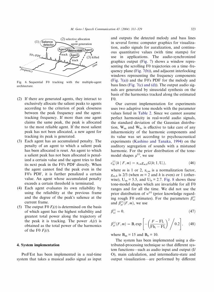
Our architecture consists of a salience detector

and multiple agents (Fig. 6). The salience detector

picks up promising salient peaks in the F0�s PDF,

and the agents driven by those peaks track their

trajectories. They behave at each frame as follows

(the first three steps correspond to the numbers inFig. 6):

(1) After forming the F0�s PDF at each frame, the

salience detector picks out several salient

peaks that are higher than a dynamic thresh-

old that is adjusted according to the maxi-

mum peak. The detector then evaluates how

promising each salient peak is by trackingits trajectory in the near future (at most 50

ms) taking into consideration the total power

transition. For the real-time implementation,

this can be done by regarding the present time

as the near-future time.

Interactiontrack

trackkilled

Agent

Agent

Agent

selective allocation

agent generationSaliencedetector

frequency

or

time

F0's PDF

(1)

(3)

(2)

Fig. 6. Sequential F0 tracking with the multiple-agent

architecture.

M. Goto / Speech Communication 43 (2004) 311–329 323

(2) If there are generated agents, they interact to

exclusively allocate the salient peaks to agents

according to the criterion of peak closenessbetween the peak frequency and the agent-

tracking frequency. If more than one agent

claims the same peak, the peak is allocated

to the most reliable agent. If the most salient

peak has not been allocated, a new agent for

tracking its peak is generated.

(3) Each agent has an accumulated penalty. The

penalty of an agent to which a salient peakhas been allocated is reset. An agent to which

a salient peak has not been allocated is penal-

ized a certain value and the agent tries to find

its next peak in the F0�s PDF directly. When

the agent cannot find the peak even in the

F0�s PDF, it is further penalized a certain

value. An agent whose accumulated penalty

exceeds a certain threshold is terminated.(4) Each agent evaluates its own reliability by

using the reliability at the previous frame

and the degree of the peak�s salience at the

current frame.

(5) The output F0 Fi(t) is determined on the basis

of which agent has the highest reliability and

greatest total power along the trajectory of

the peak it is tracking. The power Ai(t) isobtained as the total power of the harmonics

of the F0 Fi(t).

4. System implementation

PreFEst has been implemented in a real-time

system that takes a musical audio signal as input

and outputs the detected melody and bass lines

in several forms: computer graphics for visualiza-

tion, audio signals for auralization, and continu-

ous quantitative values (with time stamps) for

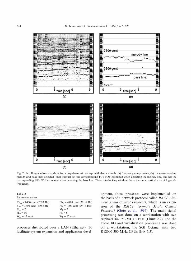
use in applications. The audio-synchronizedgraphics output (Fig. 7) shows a window repre-

senting the scrolling F0 trajectories on a time–fre-

quency plane (Fig. 7(b)), and adjacent interlocking

windows representing the frequency components

(Fig. 7(a)) and the F0�s PDF for the melody and

bass lines (Fig. 7(c) and (d)). The output audio sig-

nals are generated by sinusoidal synthesis on the

basis of the harmonics tracked along the estimatedF0.

Our current implementation for experiments

uses two adaptive tone models with the parameter

values listed in Table 2. Since we cannot assume

perfect harmonicity in real-world audio signals,

the standard deviation of the Gaussian distribu-

tion, Wm and Wb, is effective to take care of any

inharmonicity of the harmonic components andits value was set according to psychoacoustical

experiments (Kashino and Tanaka, 1994) on the

auditory segregation of sounds with a mistuned

harmonic. For the prior distribution of the tone-

model shapes l(t), we use

cðtÞ0i ðh j F ;mÞ ¼ ai;mgm;hGðh; 1;UiÞ; ð46Þ

where m is 1 or 2, ai,m is a normalization factor,

gm,h is 2/3 (when m = 2 and h is even) or 1 (other-

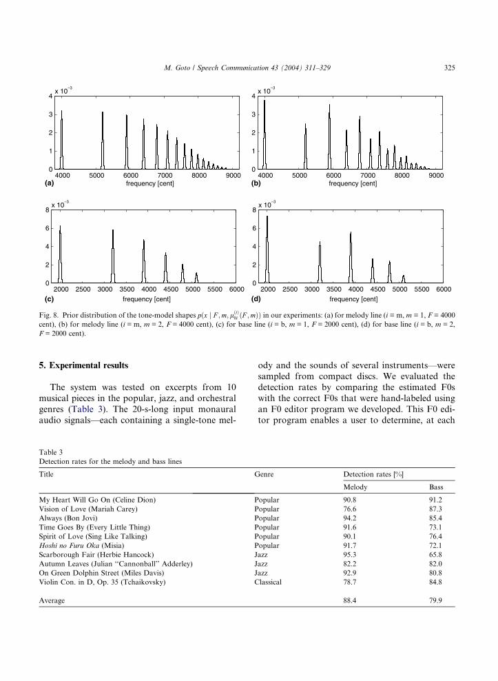
wise), Um = 5.5, and Ub = 2.7. Fig. 8 shows these

tone-model shapes which are invariable for all F0

ranges and for all the time. We did not use the

prior distribution of w(t) (prior knowledge regard-

ing rough F0 estimates). For the parameters bðtÞwi

and bðtÞli ðF ;mÞ, we use

bðtÞwi ¼ 0; ð47Þ

bðtÞli ðF ;mÞ ¼ Bi exp � F � Fli

Fhi � Fli

� �2,

0:2

" #; ð48Þ

where Bm = 15 and Bb = 10.

The system has been implemented using a dis-

tributed-processing technique so that different sys-

tem functions––such as audio input and output (I/

O), main calculation, and intermediate-state and

output visualization––are performed by different

Fig. 7. Scrolling-window snapshots for a popular-music excerpt with drum sounds: (a) frequency components, (b) the corresponding

melody and bass lines detected (final output), (c) the corresponding F0�s PDF estimated when detecting the melody line, and (d) the

corresponding F0�s PDF estimated when detecting the bass line. These interlocking windows have the same vertical axis of log-scale

frequency.

Table 2

Parameter values

Fhm = 8400 cent (2093 Hz) Fhb = 4800 cent (261.6 Hz)

Flm = 3600 cent (130.8 Hz) Flb = 1000 cent (29.14 Hz)

Mm = 2 Mb = 2

Hm = 16 Hb = 6

Wm = 17 cent Wb = 17 cent

324 M. Goto / Speech Communication 43 (2004) 311–329

processes distributed over a LAN (Ethernet). To

facilitate system expansion and application devel-

opment, those processes were implemented on

the basis of a network protocol called RACP (Re-

mote Audio Control Protocol), which is an exten-

sion of the RMCP (Remote Music Control

Protocol) (Goto et al., 1997). The main signal

processing was done on a workstation with two

Alpha21264 750-MHz CPUs (Linux 2.2), and the

audio I/O and visualization processing was done

on a workstation, the SGI Octane, with two

R12000 300-MHz CPUs (Irix 6.5).

4000 5000 6000 7000 8000 90000

1

2

3

4x 10

–3

frequency [cent]4000 5000 6000 7000 8000 9000

0

1

2

3

4x 10

–3

frequency [cent]

2000 2500 3000 3500 4000 4500 5000 5500 60000

2

4

6

8x 10

–3

frequency [cent]

2000 2500 3000 3500 4000 4500 5000 5500 60000

2

4

6

8x 10

–3

frequency [cent]

(a) (b)

(c) (d)

Fig. 8. Prior distribution of the tone-model shapes pðx j F ;m;lðtÞ0i ðF ;mÞÞ in our experiments: (a) for melody line (i = m, m = 1, F = 4000

cent), (b) for melody line (i = m, m = 2, F = 4000 cent), (c) for base line (i = b, m = 1, F = 2000 cent), (d) for base line (i = b, m = 2,

F = 2000 cent).

M. Goto / Speech Communication 43 (2004) 311–329 325

5. Experimental results

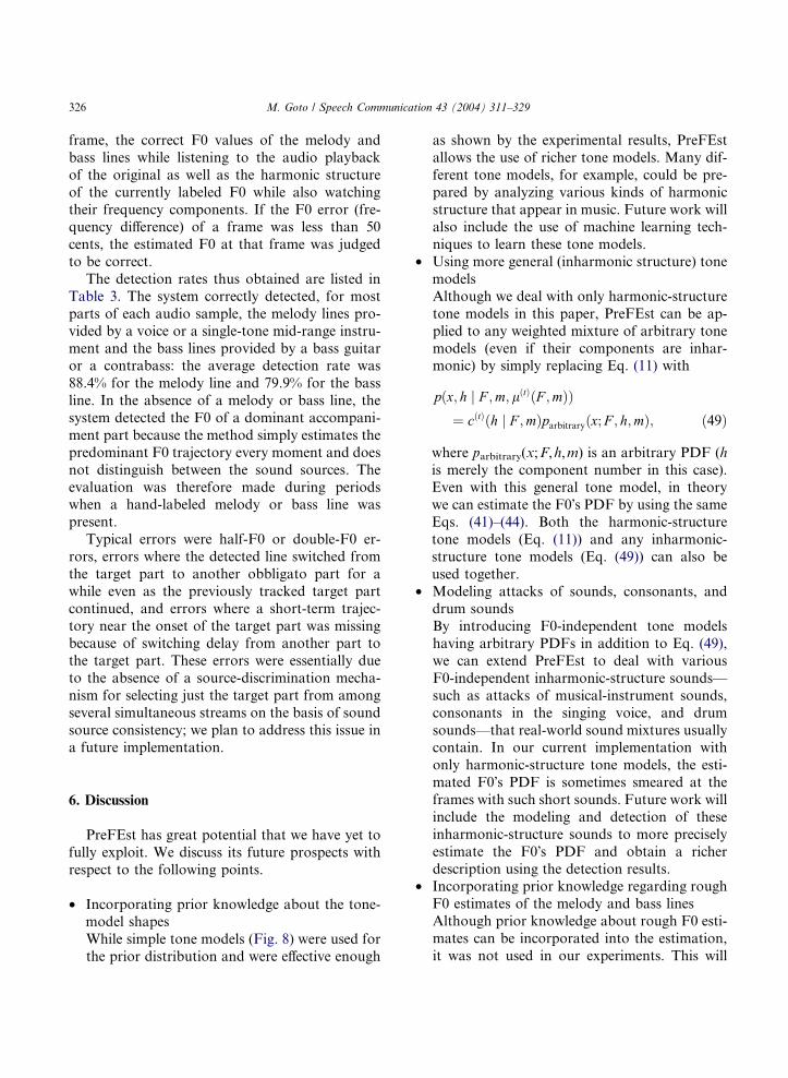
The system was tested on excerpts from 10

musical pieces in the popular, jazz, and orchestral

genres (Table 3). The 20-s-long input monaural

audio signals––each containing a single-tone mel-

Table 3

Detection rates for the melody and bass lines

Title G

My Heart Will Go On (Celine Dion) P

Vision of Love (Mariah Carey) P

Always (Bon Jovi) P

Time Goes By (Every Little Thing) P

Spirit of Love (Sing Like Talking) P

Hoshi no Furu Oka (Misia) P

Scarborough Fair (Herbie Hancock) J

Autumn Leaves (Julian ‘‘Cannonball’’ Adderley) J

On Green Dolphin Street (Miles Davis) J

Violin Con. in D, Op. 35 (Tchaikovsky) C

Average

ody and the sounds of several instruments––were

sampled from compact discs. We evaluated the

detection rates by comparing the estimated F0s

with the correct F0s that were hand-labeled using

an F0 editor program we developed. This F0 edi-

tor program enables a user to determine, at each

enre Detection rates [%]

Melody Bass

opular 90.8 91.2

opular 76.6 87.3

opular 94.2 85.4

opular 91.6 73.1

opular 90.1 76.4

opular 91.7 72.1

azz 95.3 65.8

azz 82.2 82.0

azz 92.9 80.8

lassical 78.7 84.8

88.4 79.9

326 M. Goto / Speech Communication 43 (2004) 311–329

frame, the correct F0 values of the melody and

bass lines while listening to the audio playback

of the original as well as the harmonic structure

of the currently labeled F0 while also watching

their frequency components. If the F0 error (fre-quency difference) of a frame was less than 50

cents, the estimated F0 at that frame was judged

to be correct.

The detection rates thus obtained are listed in

Table 3. The system correctly detected, for most

parts of each audio sample, the melody lines pro-

vided by a voice or a single-tone mid-range instru-

ment and the bass lines provided by a bass guitaror a contrabass: the average detection rate was

88.4% for the melody line and 79.9% for the bass

line. In the absence of a melody or bass line, the

system detected the F0 of a dominant accompani-

ment part because the method simply estimates the

predominant F0 trajectory every moment and does

not distinguish between the sound sources. The

evaluation was therefore made during periodswhen a hand-labeled melody or bass line was

present.

Typical errors were half-F0 or double-F0 er-

rors, errors where the detected line switched from

the target part to another obbligato part for a

while even as the previously tracked target part

continued, and errors where a short-term trajec-

tory near the onset of the target part was missingbecause of switching delay from another part to

the target part. These errors were essentially due

to the absence of a source-discrimination mecha-

nism for selecting just the target part from among

several simultaneous streams on the basis of sound

source consistency; we plan to address this issue in

a future implementation.

6. Discussion

PreFEst has great potential that we have yet to

fully exploit. We discuss its future prospects with

respect to the following points.

• Incorporating prior knowledge about the tone-model shapes

While simple tone models (Fig. 8) were used for

the prior distribution and were effective enough

as shown by the experimental results, PreFEst

allows the use of richer tone models. Many dif-

ferent tone models, for example, could be pre-

pared by analyzing various kinds of harmonic

structure that appear in music. Future work willalso include the use of machine learning tech-

niques to learn these tone models.

• Using more general (inharmonic structure) tone

models

Although we deal with only harmonic-structure

tone models in this paper, PreFEst can be ap-

plied to any weighted mixture of arbitrary tone

models (even if their components are inhar-monic) by simply replacing Eq. (11) with

pðx; h j F ;m; lðtÞðF ;mÞÞ¼ cðtÞðh j F ;mÞparbitraryðx; F ; h;mÞ; ð49Þ

where parbitrary(x;F,h,m) is an arbitrary PDF (his merely the component number in this case).

Even with this general tone model, in theory

we can estimate the F0�s PDF by using the same

Eqs. (41)–(44). Both the harmonic-structure

tone models (Eq. (11)) and any inharmonic-

structure tone models (Eq. (49)) can also be

used together.

• Modeling attacks of sounds, consonants, anddrum sounds

By introducing F0-independent tone models

having arbitrary PDFs in addition to Eq. (49),

we can extend PreFEst to deal with various

F0-independent inharmonic-structure sounds––

such as attacks of musical-instrument sounds,

consonants in the singing voice, and drum

sounds––that real-world sound mixtures usuallycontain. In our current implementation with

only harmonic-structure tone models, the esti-

mated F0�s PDF is sometimes smeared at the

frames with such short sounds. Future work will

include the modeling and detection of these

inharmonic-structure sounds to more precisely

estimate the F0�s PDF and obtain a richer

description using the detection results.• Incorporating prior knowledge regarding rough

F0 estimates of the melody and bass lines

Although prior knowledge about rough F0 esti-

mates can be incorporated into the estimation,

it was not used in our experiments. This will

M. Goto / Speech Communication 43 (2004) 311–329 327

be useful for some practical applications, such

as the analysis of expression in a recorded per-

formance, where a more precise F0 with fewer

errors is required.

• Tracking multiple sound sources with sound-source identification

Although multiple peaks in the F0�s PDF, each

corresponding to a different sound source, are

tracked by multiple agents in the PreFEst-

back-end, we did not fully exploit them. If they

could be tracked while considering their sound

source consistency by using a sound source

identification method, we can investigate othersimultaneous sound sources as well as the mel-

ody and bass lines. A study of integrating a

sound source identification method with tone-

model shapes in PreFEst will be necessary.

7. Conclusion

We have described the problem of music

scene description––auditory scene description in

music––and have addressed the problems regard-

ing the detection of the melody and bass lines in

complex real-world audio signals. The predomi-

nant-F0 estimation method PreFEst makes it pos-

sible to detect these lines by estimating the mostpredominant F0 trajectory. Experimental results

showed that our system implementing PreFEst

can estimate, in real time, the predominant F0s

of the melody and bass lines in audio signals sam-

pled from compact discs.

Our research shows that the pitch-related prop-

erties of real-world musical audio signals––like the

melody and bass lines––as well as temporal prop-erties like the hierarchical beat structure, can be

described without segregating sound sources. Tak-

ing a hint from the observation that human listen-

ers can easily listen to the melody and bass lines,

we developed PreFEst to detect these lines sepa-

rately by using only partial information within

intentionally limited frequency ranges. Because it

is generally impossible to know a priori the num-ber of sound sources in a real-world environment,

PreFEst considers all possibilities of the F0 at the

same time and estimates, by using the EM algo-

rithm, a probability density function of the F0

which represents the relative dominance of every

possible harmonic structure. This approach natu-

rally does not require the existence of the F0�s fre-

quency component and can handle the missingfundamental that often occurs in musical audio

signals. In addition, the multiple-agent architec-

ture makes it possible to determine the most dom-

inant and stable F0 trajectory from the viewpoint

of global temporal continuity of the F0.

In the future, we plan to work on the various

extensions discussed in Section 6. While PreFEst

was developed for music audio signals, it––espe-cially the PreFEst-core––can also be applied to

non-music audio signals. In fact, Masuda-Katsuse

(Masuda-Katsuse, 2001; Masuda-Katsuse and

Sugano, 2001) has extended it and demonstrated

its effectiveness for speech recognition in realistic

noisy environments.

Acknowledgments

I thank Shotaro Akaho and Hideki Asoh (Na-

tional Institute of Advanced Industrial Science

and Technology) for their valuable discussions. I

also thank the anonymous reviewers for their help-

ful comments and suggestions.

References

Abe, T., Kobayashi, T., Imai, S., 1996. Robust pitch estimation

with harmonics enhancement in noisy environments based

on instantaneous frequency. In: Proc. Internat. Conf. on

Spoken Language Processing (ICSLP 96), pp. 1277–1280.

Abe, T., Kobayashi, T., Imai, S., 1997. The IF spectrogram: a

new spectral representation. In: Proc. Internat. Sympos. on

Simulation, Visualization and Auralization for Acoustic

Research and Education (ASVA 97), pp. 423–430.

Boashash, B., 1992. Estimating and interpreting the instanta-

neous frequency of a signal. Proc. IEEE 80 (4), 520–568.

Bregman, A.S., 1990. Auditory Scene Analysis: The Perceptual

Organization of Sound. The MIT Press.

Brown, G.J., 1992. Computational auditory scene analysis: a

representational approach. Ph.D. thesis, University of

Sheffield.

Brown, G.J., Cooke, M., 1994. Perceptual grouping of musical

sounds: a computational model. J. New Music Res. 23, 107–

132.

328 M. Goto / Speech Communication 43 (2004) 311–329

Chafe, C., Jaffe, D., 1986. Source separation and note identi-

fication in polyphonic music. In: Proc. IEEE Internat. Conf.

on Acoustics, Speech, and Signal Processing (ICASSP 86),

pp. 1289–1292.

Charpentier, F.J., 1986. Pitch detection using the short-term

phase spectrum. In: Proc. IEEE Internat. Conf. on Acous-

tics, Speech, and Signal Processing (ICASSP 86), pp. 113–

116.

Cooke, M., Brown, G., 1993. Computational auditory scene

analysis: exploiting principles of perceived continuity.

Speech Comm. 13, 391–399.

de Cheveigne, A., 1993. Separation of concurrent harmonic

sounds: fundamental frequency estimation and a time-

domain cancellation model of auditory processing. J.

Acoust. Soc. Amer. 93 (6), 3271–3290.

de Cheveigne, A., Kawahara, H., 1999. Multiple period

estimation and pitch perception model. Speech Comm. 27

(3–4), 175–185.

Dempster, A.P., Laird, N.M., Rubin, D.B., 1977. Maximum

likelihood from incomplete data via the EM algorithm. J.

Roy. Statist. Soc. B 39 (1), 1–38.

Flanagan, J.L., Golden, R.M., 1966. Phase vocoder. Bell

System Tech. J. 45, 1493–1509.

Goto, M., 1998. A study of real-time beat tracking for musical

audio signals. Ph.D. thesis, Waseda University (in

Japanese).

Goto, M., 2001. An audio-based real-time beat tracking system

for music with or without drum-sounds. J. New Music Res.

30 (2), 159–171.

Goto, M., Muraoka, Y., 1994. A beat tracking system for

acoustic signals of music. In: Proc. 2nd ACM Internat.

Conf. on Multimedia (ACM Multimedia 94), pp. 365–372.

Goto, M., Muraoka, Y., 1996. Beat tracking based on multiple-

agent architecture––a real-time beat tracking system for

audio signals. In: Proc. 2nd Internat. Conf. on Multiagent

Systems (ICMAS-96), pp. 103–110.

Goto, M., Muraoka, Y., 1998. Music understanding at the beat

level––real-time beat tracking for audio signals. In: Com-

putational Auditory Scene Analysis. Lawrence Erlbaum

Associates, pp. 157–176.

Goto, M., Muraoka, Y., 1999. Real-time beat tracking for

drumless audio signals: chord change detection for musical

decisions. Speech Comm. 27 (3–4), 311–335.

Goto, M., Neyama, R., Muraoka, Y., 1997. RMCP: remote

music control protocol––design and applications. In: Proc.

1997 Internat. Computer Music Conference (ICMC 97),

pp. 446–449.

Kashino, K., 1994. Computational auditory scene analysis for

music signals. Ph.D. thesis, University of Tokyo (in

Japanese).

Kashino, K., Murase, H., 1997. A music stream segregation

system based on adaptive multi-agents. In: Proc. Internat.

Joint Conf. on Artificial Intelligence (IJCAI-97), pp. 1126–

1131.

Kashino, K., Tanaka, H., 1994. A computational model of

segregation of two frequency components––evaluation and

integration of multiple cues. Electron. Comm. Jpn. (Part

III) 77 (7), 35–47.

Kashino, K., Nakadai, K., Kinoshita, T., Tanaka, H., 1998.

Application of the Bayesian probability network to music

scene analysis. In: Computational Auditory Scene Analysis.

Lawrence Erlbaum Associates, pp. 115–137.

Katayose, H., Inokuchi, S., 1989. The kansei music system.

Comput. Music J. 13 (4), 72–77.

Kawahara, H., Katayose, H., de Cheveigne, A., Patterson,

R.D., 1999. Fixed point analysis of frequency to instanta-

neous frequency mapping for accurate estimation of F0

and periodicity. In: Proc. European Conf. on Speech

Communication and Technology (Eurospeech 99), pp.

2781–2784.

Kitano, H., 1993. Challenges of massive parallelism. In: Proc.

Internat. Joint Conf. on Artificial Intelligence (IJCAI-93),

pp. 813–834.

Klapuri, A.P., 2001. Multipitch estimation and sound separa-

tion by the spectral smoothness principle. In: Proc. IEEE

Internat. Conf. on Acoustics, Speech, and Signal Processing

(ICASSP 2001).

Masuda-Katsuse, I., 2001. A new method for speech recogni-

tion in the presence of non-stationary, unpredictable and

high-level noise. In: Proc. European Conf. on Speech

Communication and Technology (Eurospeech 2001), pp.

1119–1122.

Masuda-Katsuse, I., Sugano, Y., 2001. Speech estimation

biased by phonemic expectation in the presence of non-

stationary and unpredictable noise. In: Proc. Workshop on

Consistent & Reliable Acoustic Cues for Sound Analysis

(CRAC workshop).

Nakatani, T., Okuno, H.G., Kawabata, T., 1995. Residue-

driven architecture for computational auditory scene anal-

ysis. In: Proc. Internat. Joint Conf. on Artificial Intelligence

(IJCAI-95), pp. 165–172.

Nehorai, A., Porat, B., 1986. Adaptive comb filtering for

harmonic signal enhancement. IEEE Trans. ASSP ASSP-34

(5), 1124–1138.

Noll, A.M., 1967. Cepstrum pitch determination. J. Acoust.

Soc. Amer. 41 (2), 293–309.

Ohmura, H., 1994. Fine pitch contour extraction by voice

fundamental wave filtering method. In: Proc. IEEE Inter-

nat. Conf. on Acoustics, Speech, and Signal Processing

(ICASSP 94), pp. II–189–192.

Okuno, H.G., Cooke, M.P. (Eds.), 1997. Working Notes of the

IJCAI-97 Workshop on Computational Auditory Scene

Analysis.

Parsons, T.W., 1976. Separation of speech from interfering

speech by means of harmonic selection. J. Acoust. Soc.

Amer. 60 (4), 911–918.

Plomp, R., 1967. Pitch of complex tones. J. Acoust. Soc. Amer.

41 (6), 1526–1533.

M. Goto / Speech Communication 43 (2004) 311–329 329

Rabiner, L.R., Cheng, M.J., Rosenberg, A.E., McGonegal,

C.A., 1976. A comparative performance study of several

pitch detection algorithms. IEEE Trans. ASSP ASSP-24 (5),

399–418.

Ritsma, R.J., 1967. Frequencies dominant in the perception of the

pitch of complex sounds. J. Acoust. Soc. Amer. 42 (1), 191–198.

Rosenthal, D., Okuno, H.G. (Eds.), 1995. Working Notes of

the IJCAI-95 Workshop on Computational Auditory Scene

Analysis.

Rosenthal, D.F., Okuno, H.G. (Eds.), 1998. Computa-

tional Auditory Scene Analysis. Lawrence Erlbaum

Associates.

Schroeder, M.R., 1968. Period histogram and product spec-

trum: new methods for fundamental-frequency measure-

ment. J. Acoust. Soc. Amer. 43 (4), 829–834.

Tolonen, T., Karjalainen, M., 2000. A computationally efficient

multipitch analysis model. IEEE Trans. Speech Audio

Process. 8 (6), 708–716.