A Real-Time, Three-Dimensional, Rapidly Updating ...€¦ · A Real-Time, Three-Dimensional,...

A Real-Time, Three-Dimensional, Rapidly Updating, Heterogeneous Radar MergerTechnique for Reflectivity, Velocity, and Derived Products

VALLIAPPA LAKSHMANAN AND TRAVIS SMITH

Cooperative Institute of Mesoscale Meteorological Studies, University of Oklahoma, and National Severe Storms Laboratory,Norman, Oklahoma

KURT HONDL

National Severe Storms Laboratory, Norman, Oklahoma

GREGORY J. STUMPF

Cooperative Institute of Mesoscale Meteorological Studies, University of Oklahoma, Norman, Oklahoma, and MeteorologicalDevelopment Laboratory, National Weather Service, Silver Spring, Maryland

ARTHUR WITT

National Severe Storms Laboratory, Norman, Oklahoma

(Manuscript received 5 April 2005, in final form 18 January 2006)

ABSTRACT

With the advent of real-time streaming data from various radar networks, including most WeatherSurveillance Radars-1988 Doppler and several Terminal Doppler Weather Radars, it is now possible tocombine data in real time to form 3D multiple-radar grids. Herein, a technique for taking the base radardata (reflectivity and radial velocity) and derived products from multiple radars and combining them in realtime into a rapidly updating 3D merged grid is described. An estimate of that radar product combined fromall the different radars can be extracted from the 3D grid at any time. This is accomplished through aformulation that accounts for the varying radar beam geometry with range, vertical gaps between radarscans, the lack of time synchronization between radars, storm movement, varying beam resolutions betweendifferent types of radars, beam blockage due to terrain, differing radar calibration, and inaccurate timestamps on radar data. Techniques for merging scalar products like reflectivity, and innovative, real-timetechniques for combining velocity and velocity-derived products are demonstrated. Precomputation tech-niques that can be utilized to perform the merger in real time and derived products that can be computedfrom these three-dimensional merger grids are described.

1. Introduction

The Weather Surveillance Radar-1988 Doppler(WSR-88D) network now covers most of the continen-tal United States, and full-resolution base data fromnearly all the WSR-88D radars are compressed usingblock encoding (Burrows and Wheeler 1994) and trans-mitted in real time to interested users (Droegemeier et

al. 2002). This makes it possible for clients of this datastream to consider combining the information frommultiple radars to alleviate problems arising from radargeometry (cone of silence, beam spreading, beamheight, beam blockage, etc.). Greater accuracy in radarmeasurements can be achieved by oversamplingweather signatures using more than one radar.

In addition, data from several Terminal DopplerWeather Radars (TDWRs) are being transmitted inreal time. Because the TDWRs provide higher spatialresolution close to urban areas, it is advantageous toincorporate them into the merged grids as well. Theradar network resulting from the National Science

Corresponding author address: Valliappa Lakshmanan,CIMMS, OU/NSSL, 120 David L. Boren Blvd., Norman, OK73072.E-mail: [email protected]

802 W E A T H E R A N D F O R E C A S T I N G VOLUME 21

© 2006 American Meteorological Society

WAF942

Foundation–sponsored Center for the CollaborativeAdaptive Sensing of the Atmosphere (CASA) prom-ises to provide data to fill out the �3 km umbrella ofthe Next-Generation Weather Radar network (Brotzgeet al. 2005). Developing a real-time heterogeneous ra-dar data combination technique is essential to the util-ity of the CASA network.

Further, with the advent of phased-array radars withno set volume coverage patterns and the possibility ofhighly adaptive scanning strategies, a real-time, three-dimensional, rapidly updating merger technique toplace the scanned data into a earth-relative context isextremely important for downstream applications ofthe data.

A combination of information from multiple radarshas typically been attempted in two dimensions. Forexample, the National Weather Service creates a 10-kmnational reflectivity mosaic (Charba and Liang 2005).We, however, are interested in creating a 3D combinedgrid because such a 3D grid would be suitable for cre-ating severe weather algorithm products and for deter-mining the direction individual CASA radars need topoint.

Spatial interpolation techniques used to create 3Dmultiple-radar grids have been examined by Trapp andDoswell (2000) and Askelson et al. (2000). Zhang et al.(2005) consider spatial interpolation techniques fromthe point of retaining, as much as possible, the under-lying storm structures evident in the single-radar data.Specifically, they show that a technique with the fol-lowing characteristics suffices to create spatially smoothmultiradar 3D mosaics: (a) nearest-neighbor mappingin range and azimuth, (b) linear vertical or bilinear ver-tical–horizontal interpolation, and (c) weighting indi-vidual range gates’ reflectivity values with an exponen-tial function of distance. In this paper, we build uponthose results by describing the following:

1) how to combine the data using “virtual volumes”—a rapidly updating grid such that the merged gridhas an (theoretically) infinitesimal temporal resolu-tion;

2) how to account for time asynchronicity between ra-dars;

3) a technique of precomputations in order to keep thelatency down to a fraction of a second;

4) extracting subdomain precomputations from largerprecomputations in order to create domains ofmerged radar products on demand;

5) a real-time technique of combining not just radarreflectivity data, but also velocity data; and

6) the derivation of multiple-radar algorithm prod-ucts.

a. Motivation

Many radar algorithms are currently written to workwith data from a single radar. However, such algo-rithms for everything from estimating hail sizes to esti-mating precipitation can perform much better if datafrom nearby radars and other sensors are considered.Using data from other radars would help mitigate radargeometry problems, achieve a much better verticalresolution, attain much better spatial coverage, and ob-tain data at faster time steps. Figure 1 demonstrates acase where information on vertical structure was un-available from the closest radar, but where the use ofdata from adjacent radars filled in that information.Using data from other sensors and numerical modelswould help provide information about the near-stormenvironment and temperature profiles. Considering thenumerous advantages of using all of the available datain conjunction, and considering that technology hasevolved to the point where such data can be transmittedand effectively used in real time, there is little reason toconsider single-radar vertical integrated liquid (VIL) orhail diagnosis.

b. Challenges in merging radar data

One of the challenges with merging data from mul-tiple radars is that radars within the WSR-88D networkare not synchronized. First, the clocks of the radars arenot in sync. This problem will be fixed in the next majorupgrade to the radar signal processors. A challengefaced by algorithms that integrate data from multipleradars is that the radar scanning strategies are not thesame. Thus, a radar in Nebraska might be in precipita-tion mode, scanning 11 tilt angles every 5 min, while theadjacent radar in Kansas might be in clear-air mode,scanning just 5 angles every 10 min. Of course, this isactually beneficial. If the radar volume coverage pat-terns (VCPs) were synchronized, then we would not beable to sample storms from multiple radars at differentheights almost simultaneously (because, in general, thesame storm will be at different distances from differentradars). Therefore, as opposed to the WSR-88D net-work radars being synchronized, it would be beneficialif the nonsynchronicity was actually planned, in theform of multiradar adaptive strategies.

As a result of radar beam geometry, each range gatefrom each radar contributes to the final grid value atmultiple points within a 3D dynamic grid. Becausesome of the data might be 10 min old, while other datamight be only a few seconds old, a naive combination ofdata will result in spatial errors. Therefore, the rangegate data from the radars need to be advected based ona time synchronization with the resulting 3D grid. The

OCTOBER 2006 L A K S H M A N A N E T A L . 803

FIG. 1. Using data from multiple nearby radars can mitigate the cone of silence and other radar geometry issues.(a) A vertical slice through a full volume of data from the Dyess Air Force Base, TX (KDYX), radar on 6 Feb 2005.Note the cone of silence; this is information unavailable to applications processing only KDYX data. (b) The lowestelevation scan from the KDYX radar. (c) An equivalent vertical slice through the merged data from KDYX;Frederick, OK (KFDR); Lubbock, TX (KLBB); Midland, TX (KMAF); and San Angelo, TX (KSJT). Nearbyradars have filled in the cone of silence from KDYX. (d) A horizontal slice at 3 km above mean sea level throughthe merged data.


data need to be moved to the position in which thestorm is anticipated to be. This adjustment is differentfor each point in the 3D grid. At any one point on the3D grid there could be multiple radar estimates fromeach of the different radars.

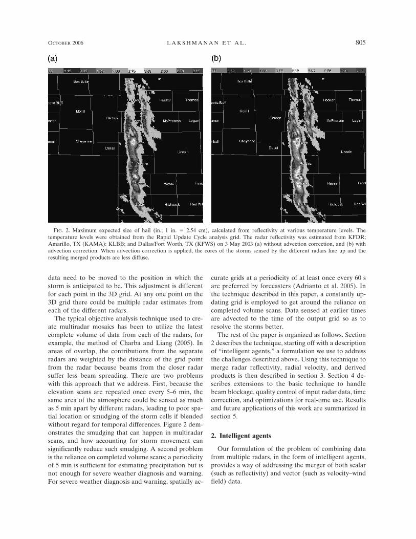
The typical objective analysis technique used to cre-ate multiradar mosaics has been to utilize the latestcomplete volume of data from each of the radars, forexample, the method of Charba and Liang (2005). Inareas of overlap, the contributions from the separateradars are weighted by the distance of the grid pointfrom the radar because beams from the closer radarsuffer less beam spreading. There are two problemswith this approach that we address. First, because theelevation scans are repeated once every 5–6 min, thesame area of the atmosphere could be sensed as muchas 5 min apart by different radars, leading to poor spa-tial location or smudging of the storm cells if blendedwithout regard for temporal differences. Figure 2 dem-onstrates the smudging that can happen in multiradarscans, and how accounting for storm movement cansignificantly reduce such smudging. A second problemis the reliance on completed volume scans; a periodicityof 5 min is sufficient for estimating precipitation but isnot enough for severe weather diagnosis and warning.For severe weather diagnosis and warning, spatially ac-

curate grids at a periodicity of at least once every 60 sare preferred by forecasters (Adrianto et al. 2005). Inthe technique described in this paper, a constantly up-dating grid is employed to get around the reliance oncompleted volume scans. Data sensed at earlier timesare advected to the time of the output grid so as toresolve the storms better.

The rest of the paper is organized as follows. Section2 describes the technique, starting off with a descriptionof “intelligent agents,” a formulation we use to addressthe challenges described above. Using this technique tomerge radar reflectivity, radial velocity, and derivedproducts is then described in section 3. Section 4 de-scribes extensions to the basic technique to handlebeam blockage, quality control of input radar data, timecorrection, and optimizations for real-time use. Resultsand future applications of this work are summarized insection 5.

2. Intelligent agents

Our formulation of the problem of combining datafrom multiple radars, in the form of intelligent agents,provides a way of addressing the merger of both scalar(such as reflectivity) and vector (such as velocity–windfield) data.

FIG. 2. Maximum expected size of hail (in.; 1 in. � 2.54 cm), calculated from reflectivity at various temperature levels. Thetemperature levels were obtained from the Rapid Update Cycle analysis grid. The radar reflectivity was estimated from KFDR;Amarillo, TX (KAMA): KLBB; and Dallas/Fort Worth, TX (KFWS) on 3 May 2003 (a) without advection correction, and (b) withadvection correction. When advection correction is applied, the cores of the storms sensed by the different radars line up and theresulting merged products are less diffuse.


Intelligent agents, sometimes called autonomousagents, are computational systems that inhabit somecomplex dynamic environment, sense and act autono-mously in this environment, and by doing so realize aset of goals or tasks for which they are designed (Maes1995). Smith et al. (1994) concisely characterize intelli-gent agents as persistent entities that are dedicated tospecific purposes—the persistence requirement differ-entiates agents from formulas [Smith et al. (1994) usethe term “subroutine”] because formulas are not longlived. The specific purpose characterization differenti-ates them from more complex “multifunction” algo-rithms.

In the context of merging radar data from multiple,possibly heterogeneous radars, each range gate of theradar serves as the impetus for the creation of one ormore intelligent agents. Each intelligent agent monitorsthe movement of the storm at the position that it iscurrently in, and finds a place in the resulting grid basedon time difference. Then, at the next time instant, therange gate migrates to its new position in the grid. Theagents remove themselves when they expect to havebeen superseded. When new storm motion estimatesare available, the agent updates itself with the new mo-tion vector. When multiple agents all have an answerfor a given point in the 3D grid, they collaborate tocome up with a single value following strategies speci-fied by the end user. These strategies may correspondto typical objective-analysis weighting schemes or tech-niques more suitable to the actual product beingmerged.

It should be clear that in the absence of time correc-tion via advection of older data, the intelligent agenttechnique resolves directly to objective-analysis or mul-tiple-Doppler techniques. Thus, the mathematical for-mulas in this paper will be presented in those moretraditional terms.

The use of intelligent agents creates a flexible, scal-able system that is not bogged down even by a highly“weather active” domain (e.g., a hurricane where mostradar grid points have significant power returns). Thistechnique of using an intelligent agent for each rangegate with data from every radar in a given domain wasproven to be robust and scalable even during Hurri-canes Frances and Ivan in Florida (September 2004).The intelligent agents (about 1.3 million of them at onetime) all collaborated flawlessly to create the high-resolution mosaic of data, shown in Fig. 3, of HurricaneIvan from six different radars in Florida. Since the hur-ricane is over water and quite far from the coastline, noindividual radar could have captured as much of thehurricane as the merged data have.

a. Agent model

Each range gate of the radar with a valid value servesas the impetus to the creation of one or more intelligentagents. The radar-pointing azimuths, often termed“rays” or “radials,” are considered objects within a ra-dar volume that is constantly updating, and possiblywith no semblance of regularity. Not relying on theregularity of radials is necessary to be able to combinedata from phased-array radars (McNellis et al. 2005)and adaptive scanning strategies (Brotzge et al.2005).

When an agent is created, it extracts some informa-tion from the underlying radial: (a) its coordinates inthe radar-centric spherical coordinate system (range,azimuth, and elevation angle), (b) the radial start time,and (c) the radar the observation came from. Allthis information is typically available in the radar dataregardless of the type of radar or the presence or ab-sence of “volume coverage patterns.” The agent’s co-ordinates in the earth-centric latitude–longitude–heightcoordinate system of the resulting 3D grid have to becomputed, however. The agents obtain these values fol-lowing the 4/3 effective earth-radius model of Doviakand Zrnic (1993) (assuming standard beam propaga-tion).

For a grid point in the resulting 3D grid (“voxel”) atlatitude �g, longitude �g, and height hg above meansea level, the range gate that fills it, under standard

FIG. 3. Image of Hurricane Ivan consisting of combined datafrom six WSR-88D radars [Lake Charles, LA (KLCH); New Or-leans/Baton Rouge (KLIX); Mobile, AL (KMOB); Tallahassee,FL (KTLH); Tampa Bay, FL (KTBW); and Key West, FL(KBYX)]. The images were created from the latest availableWSR-88D data every 60 s (at approximately 1 km � 1 km � 1 kmresolution).


atmospheric conditions, is the range gate that is adistance r from the radar [located at (�r, �r, hr) in3D space] on a radial at an angle a from due northand on a scan tilted e to the earth’s surface where a isgiven by

a � sin�1�sin��2 � �g sin��g � �r� sin�s�R,

�1

where R is the radius of the earth and s is the great-circle distance, given by (Beyer 1987)

s � R cos�1�cos��2 � �r cos��2 � �g � sin��2 � �r sin��2 � �g cos��g � �r. �2

The elevation angle e is given by (Doviak and Zrnic1993)

e � tan�1

cos�s�IR �IR

IR � hg � hr

sin�s�IR, �3

where I is the index of refraction, which under the samestandard atmospheric conditions may be assumed to be4/3 (Doviak and Zrnic 1993), and the range r is given by

r � sin�s�IR�IR � hg � hr� cos�e. �4

Because the sin�1 function has a range of [��, �],the azimuth a is mapped to the correct quadrant ([0,2�]) by considering the signs of �g � �r and �g � �r.The voxel at �g, �g, hg can be affected by any range gatethat includes (a, r, e).

An agent’s life cycle depends on the radar scan. If theradar does not change its VCP, an agent can expect tobe replaced Ttot � Ti � Tlat later, where Ttot is theexpected length of the volume scan, Ti the time taken tocollect the scan that the agent belongs to, and Tlat is thelatency in arrival of the scan after it has been collected.In practice, Tlat is estimated to be on the same order asTi, because otherwise, it would not be possible to keepup with the data stream. At the end of its life cycle, theagent destroys itself. The time of the latest input radardata is used as the current time. If the radar VCPchanges, there will be redundant agents if the period-icity of the VCPs decreases (because the older agentswill be around a tad longer). On the other hand, if theperiodicity lengthens, there will be a short interval oftime with no agents. Because VCPs are set up such thatperiodicity decreases with the onset of weather andlengthens when weather moves away, there is no prob-lem as long as the technique can reliably deal with re-dundant agents from the same radar. Redundant agentsfrom the same radar can be dealt with using a time-weighting mechanism. By explicitly building in an al-lowance for redundant agents, radars with nonstandardscanning strategies such as a phased-array radar canoversample certain regions temporally and sense otherregions less often.

Whenever an output 3D grid is desired, all of the

existing agents collaborate to create the 3D grid. Be-cause heterogeneous radar networks are typically notsynchronized, the agents will have to account for timedifferences. Naively combining all the data at a particu-lar grid location in latitude–longitude–height space willlead to older data from one radar being combined withnewer data from another radar. This will lead to prob-lems in the initiation and decay phases of storms result-ing in severe problems in the case of fast-movingstorms. The agents, therefore, move to where they ex-pect to be at the time of the grid. For example, an agentcorresponding to a radar scan t seconds ago wouldmove to x1, y1, where

x1 � x � uxy � ty1 � y � �xy � t, �5

where x, y are the coordinates obtained from the rawazimuth–range–elevation values, and uxy, xy are hori-zontal motion vectors at x, y (scaled to the units of thegrid). Because of the difficulty of obtaining a verticalmotion estimate, the vertical motion is assumed to bezero. The motion estimate may be obtained either froma numerical model or from a radar-based tracking tech-nique such as in Lakshmanan et al. (2003b). We use thelatter in the results reported in this paper.

b. Virtual volume

Whenever a new elevation scan is received from anyof the radars contributing to the 3D grid, a set of agentsis created. The elevation scan radial data are scale fil-tered to fit the resolution of the target 3D grid. Forexample, if the radial data are at 0.25-km resolution butthe 3D grid is at a 1-km resolution, a moving average offour gates is used to yield the effective elevation scan atthe desired scale. Instead of creating an agent corre-sponding to each range gate with valid values, we invertthe problem and create an agent for each voxel in the3D latitude–longitude–height grid that each such rangegate impacts. The influence of a range gate from thecenter of the range gate extends to half the beamwidth


in the azimuthal direction and half the gate width in therange direction. This is a nearest-neighbor analysis inthe azimuth and range directions. In the elevation di-rection, the influence of this observation is given by �e,where

�e � exp��3ln�0.005, with

� �e � �i

|�i � 1 � �i|Vbi. �6

Here, � is the angular separation of the voxel from thecenter of the beam of an elevation scan (at elevation e)as a fraction either of the angular distance to the nexthigher or lower beam or the beamwidth. The V is amaximum operation, bi the beamwidth of the elevationscan, and �i the elevation angle of its center. This func-tion, shown in Fig. 4, is motivated by the fact that it is1 at the center of the beam, goes to 0.5 at half-beamwidth, and falls to below 0.01 at the beamwidth(beyond which the influence of the range gate can bedisregarded). It can be seen that where the elevationweight �e is less than 0.5, the voxel is outside the effec-tive beamwidth of the radial. Points within the effectivebeamwidth are weighted more than they would be in alinear weighting scheme. The direction of the weightingis neither vertical nor horizontal, but tangential to thedirection of the beam.

It should be noted that this interpolation is in thespherical coordinate system, in a direction orthogonalto the range–azimuth plane. Zhang et al. (2005) inter-polate either in the vertical or in both the vertical andhorizontal directions (i.e., in the coordinate system ofthe resulting 3D grid). Our technique is more efficientcomputationally, but could fail in the presence of strongvertical gradients such as bright bands, stratiform rain,

or convective anvils. Figure 5 demonstrates one casewhere spherical coordinate interpolation may suffice,but closer examination of a larger number of cases isneeded. The optimal method for interpolation might beneither the spherical interpolation nor the vertical–horizontal interpolation, but to interpolate in a direc-tion normal to the gradient direction (in 3D space).

3. Combining radar data

The methodology of performing objective analysis onradar reflectivity data is relatively clear. In section 2, weintroduced a formulation of interpolating radar dataonto a uniform grid that can address problems thatarise in being able to perform the required computa-tions in real time. In this section, we describe the ap-plication of the formulation described above to com-bining radar reflectivity, radial velocity, and derivedproducts.

a. Combining scalar data

All of the intelligent agents that impact a particularvoxel need to collaborate to determine the value at thatvoxel. In the case of scalar data, if each intelligent agentis aware of its influence weight, this reduces to deter-mining a weighted average. The agent can determine itsweight simply as an exponentially declining function ofits distance from the radar. However, there could bemultiple agents from the same radar that affect a voxel.In the case of a radar like TDWR, there could be mul-tiple scans at the same elevation angle within a volume

FIG. 4. Weighting function for interpolation between the cen-ters of radar beams; � is the fraction of the distance to the nexthigher or lower beam.

FIG. 5. Interpolation in the spherical coordinate system miti-gates brightband effects in this stratiform event. The data are fromKDYX, KFDR, KLBB, KMAF, and KSJT on 6 Feb 2005.


scan. In the case of voxels that do not lie within a beam-width, there may be two agents corresponding to theadjacent elevation scans that straddle this voxel. Also,decaying or slowly moving storms often pile up agentsinto the same voxel because of the resolution of the gridpoints. Using all of these observations together, regard-less of the reason that there are multiple agents fromthe same radar, should lead to a statistically more validestimate.

There are two broad strategies for resolving theproblem of having multiple observations (agents) fromthe same radar. One strategy is to devise a best estimatefrom each radar and then combine these estimates intoan estimate for all the radars. The other is to combineall the agents regardless of the radar from which theycome. In the case of velocity data, we use the formertechnique, while in the case of scalar data, the source ofthe data is ignored. However, to mitigate the problemof multiple, repeated elevation scans, the data areweighted both by time and distance. The influenceweight of an observation is given by

� � �eexp��t2r2��, �7

where �e is the elevation angle weight [see Eq. (6)]; t isthe time difference between the time the agent wascreated (when the radar observation was made) and thetime of the grid; r is the range of the range gate fromwhich this observation was extracted; and � is a con-stant of 17.36 s2 km2, a number that was chosen throughexperimentation. Among a range of factors that wetried, this value seemed to provide the smoothest tran-sitions while retaining much of the resolution of theoriginal data.

The weighted sum of all the observations that impacta voxel is then assigned to that voxel in the 3D grid.This grid is used for subsequent severe weather productcomputations.

b. Combining velocity data

Unlike the methodology of combining scalar data,the methodology of combining velocity data in realtime is not clear. Traditional multi-Doppler wind fieldretrieval is computationally intractable, because of itsreliance on numerical convergence. In this paper, wepresent the following three potential solutions to thisproblem: (a) computing an “inverse” velocity azimuthdisplay (VAD); (b) performing a multi-Doppler analy-sis, with certain approximations in order to keep it trac-table; and (c) forgoing the wind field retrieval alto-gether, but merging shear, a scalar field derived fromthe velocity data. All three of the above techniques areapplied after dealiasing the velocity data. For both the

WSR-88D and TDWR data, we apply the operationalWSR-88D dealiasing algorithm. The intelligent agentsused for combining the velocity data are created in thesame manner as in the case of combining scalar data,but their collaborative technique is not an objectiveanalysis one.

The multi-Doppler technique is based on the over-determined dual-Doppler technique of Kessinger et al.(1987). The terminal velocity was estimated from theequivalent radar reflectivity factor (Foote and duToit1969). We initially attempted a full 3D version of themulti-Doppler technique, because severe storms docontain regions of strong vertical motion, and it wouldbe advantageous to estimate the full 3D wind field.Unfortunately, test results for the full 3D techniquewere unsatisfactory. The vertical velocities in that tech-nique, computed via the mass continuity equation,turned out to be numerically unstable and propagatederrors into the horizontal wind fields. Instead of aban-doning the process entirely, we decided to try a simpli-fied version of the technique, which assumes that w �0. Despite the fact that this assumption of w � 0 will notbe valid for some regions of severe storms, initial testresults for this 2D version of the technique were prom-ising (Witt et al. 2005). Test results for the 2D versionof the technique on two severe weather cases showedvery good agreement between the calculated horizontalwind field and the corresponding radial velocity data.The 2D wind field also closely matched what concep-tual models of the airflow in severe storms would sug-gest.

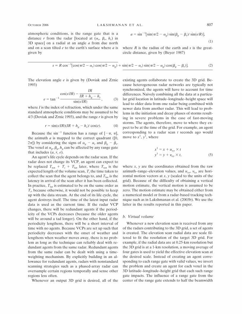
An example of merging reflectivity and velocity datafrom two heterogeneous radars—a WSR-88D at Okla-homa City/Twin Lakes, Oklahoma (KTLX), and theOklahoma City, Oklahoma (OKC), TDWR—is shownin Fig. 6. A single horizontal level, at 1.5 km abovemean sea level, is shown for the merged products. Itshould be noted that the reflectivity images from thetwo radars, KTLX and OKC, are different because theKTLX scan is 5 min older than the OKC one and thestorm has moved in the time interval. The merged radargrid does have the storm in the right location at thereference time. Note also that the wind field retrievalhas correctly identified the rotation signature.

Because the vertical motion computed from an over-determined dual-Doppler technique is not useful, wesought to examine if a more direct way of computing2D horizontal wind fields from the radar data was fea-sible. The VAD technique may be used to estimate theU and V wind components from the radial velocity ob-servations using a discrete Fourier transform (Lher-mitte and Atlas 1961; Browning and Wexler 1968;Rabin and Zrnic 1980). The VAD technique uses a


least squares approximation to calculate the first har-monic from the radial velocity observations at differentazimuths as observed from the radar location. The in-verse VAD technique similarly uses a least squares so-lution to determine the 2D wind components at a pointin space from the radial velocity observations from dif-ferent azimuths (i.e., as observed from different ra-dars).

The radial velocity observed from the ith radar i isdependent on the wind components uo and o and theobserving angles �i of the radars,

Vn�1 � Pn�2�uo�oT, �8

where

Vn�1 � ��1, �2, �3, . . . , �nT �9

and Pn�2 is given by

�sin�1 cos�1

sin�2 cos�2

· · · · · ·

sin�n cos�n

� . �10

If one has the radial velocity observations and theazimuth of the observations, a least squares approxima-tion of the wind components may be estimated using aleast squares formulation as

�uo�oT � �Pn�2T Pn�2�1�Pn�2

T Vn�1. �11

FIG. 6. A multi-Doppler wind field retrieval is shown superim-posed on data from two component radars: KTLX, which is aWSR-88D, and OKC, which is a TDWR. (a) Reflectivity fromOKC on 8 May 2003 at 2235 UTC, (b) velocity from OKC, and (c)reflectivity from KTLX. The data from KTLX are from a time 4min earlier than that of the OKC radar. (d) Velocity from KTLXand (e) merged reflectivity and wind field at 1.5 km above meansea level. The range rings from the radars are 5 km apart.


The inverse VAD technique is viable as long as thereare some radial velocity observations from nearly or-thogonal angles.

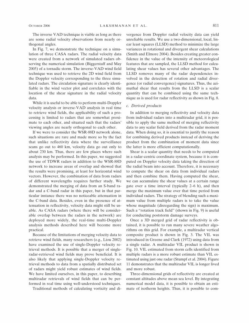
In Fig. 7, we demonstrate the technique on a simu-lation of three CASA radars. The radial velocity datawere created from a network of simulated radars ob-serving the numerical simulation (Biggerstaff and May2005) of a tornadic storm. The inverse-VAD wind fieldtechnique was used to retrieve the 2D wind field fromthe Doppler velocity corresponding to the three simu-lated radars. The circulation signature is clearly identi-fiable in the wind vector plot and correlates with thelocation of the shear signature in the radial velocitydata.

While it is useful to be able to perform multi-Dopplervelocity analysis or inverse-VAD analysis in real timeto retrieve wind fields, the applicability of such a pro-cessing is limited to radars that are somewhat proxi-mate to each other, and situated such that the radars’viewing angles are nearly orthogonal to each other.

If we were to consider the WSR-88D network alone,such situations are rare and made more so by the factthat unlike reflectivity data where the surveillancescans go out to 460 km, velocity data go out only toabout 230 km. Thus, there are few places where suchanalysis may be performed. In this paper, we suggestedthe use of TDWR radars in addition to the WSR-88Dnetwork to increase areas of overlap and showed thatthe results were promising, at least for horizontal windvectors. However, the combination of data from radarsof different wavelengths requires further study. Wedemonstrated the merging of data from an S-band ra-dar and a C-band radar in this paper, but in that par-ticular instance there was no noticeable attenuation inthe C-band data. Besides, even in the presence of at-tenuation in reflectivity, velocity data might still be us-able. As CASA radars (where there will be consider-able overlap between the radars in the network) aredeployed more widely, the real-time multi-Doppleranalysis methods described here will become morepractical.

Because of the limitations of merging velocity data toretrieve wind fields, many researchers (e.g., Liou 2002)have examined the use of single-Doppler velocity re-trieval methods. It is possible that a merger of single-radar-retrieved wind fields may prove beneficial. It isalso likely that applying single-Doppler velocity re-trieval methods to data from a spatially distributed setof radars might yield robust estimates of wind fields.We have limited ourselves, in this paper, to describingmultiradar retrievals of wind fields that can be per-formed in real time using well-understood techniques.

Traditional methods of calculating vorticity and di-

vergence from Doppler radial velocity data can yieldunreliable results. We use a two-dimensional, local, lin-ear least squares (LLSD) method to minimize the largevariances in rotational and divergent shear calculations(Smith and Elmore 2004). Besides creating greater con-fidence in the value of the intensity of meteorologicalfeatures that are sampled, the LLSD method for calcu-lating shear values has several other advantages. TheLLSD removes many of the radar dependencies in-volved in the detection of rotation and radial diver-gence (or radial convergence) signatures. Thus, the azi-muthal shear that results from the LLSD is a scalarquantity that can be combined using the same tech-nique as is used for radar reflectivity as shown in Fig. 8.

c. Derived products

In addition to merging reflectivity and velocity datafrom individual radars into a multiradar grid, it is pos-sible to apply the same method of merging reflectivitydata to any scalar field derived from the radar momentdata. When doing so, it is essential to justify the reasonfor combining derived products instead of deriving theproduct from the combination of moment data sincethe latter is more efficient computationally.

Shear is a scalar quantity that needs to be computedin a radar-centric coordinate system, because it is com-puted on Doppler velocity data taking the direction ofthe radial beam into account. Therefore, it is necessaryto compute the shear on data from individual radarsand then combine them. Having computed the shear,we can accumulate the shear values at a certain rangegate over a time interval (typically 2–6 h), and thenmerge the maximum value over that time period fromindividual radars. The strategy of blending such a maxi-mum value from multiple radars is to take the valuewhose magnitude (disregarding the sign) is maximum.Such a “rotation track field” (shown in Fig. 9) is usefulfor conducting poststorm damage surveys.

Once a 3D merged grid of radar reflectivity is ob-tained, it is possible to run many severe weather algo-rithms on this grid. For example, a multiradar verticalcomposite product is shown in Fig. 3. The VIL wasintroduced in Greene and Clark (1972) using data froma single radar. A multiradar VIL product is shown inFig. 10. VIL estimated from storm cells identified frommultiple radars is a more robust estimate than VIL es-timated using just one radar (Stumpf et al. 2004). Figure11 demonstrates that the multiradar VIL is longer livedand more robust.

Three-dimensional grids of reflectivity are created atconstant altitudes above mean sea level. By integratingnumerical model data, it is possible to obtain an esti-mate of isotherm heights. Thus, it is possible to com-


FIG. 7. An inverse-VAD wind field retrieval is shown superimposed on data from the component radars. (left) Reflectivity and (right)velocity are from simulated CASA radars (top) east, (middle) west, and (bottom) north of the area of interest. The range rings are at5-km intervals. Note that the wind field retrieved using the inverse-VAD technique has captured the thunderstorm’s rotation.


FIG. 8. (a) Vertical slice through the azimuth shear computed from a volume of datafrom the KLBB radar on 3 May 2003. (b) Azimuthal shear computed from a singleelevation scan. (c) Vertical slice through the multiradar merged azimuthal shear fromKFDR, KAMA, KLBB, and KFWS. (d) A 6-km horizontal slice through the multiradardata.


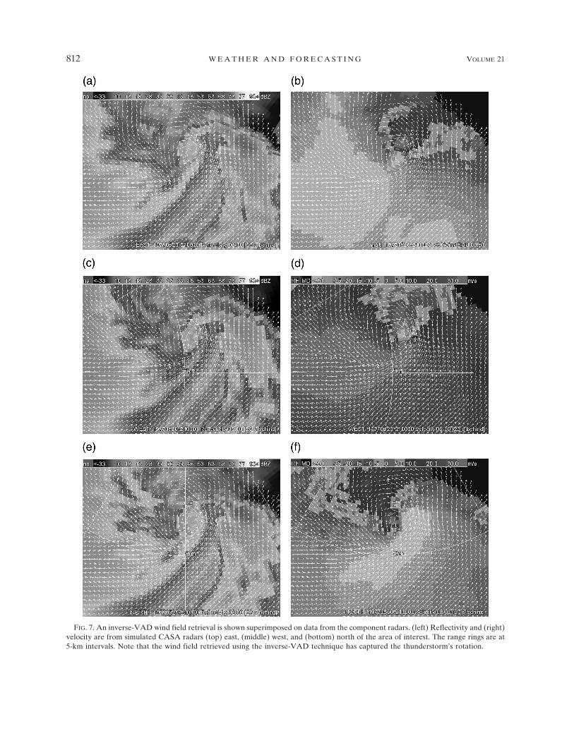
pute the reflectivity value from multiple radars and in-terpolate it to points not on a constant-altitude plane,but on a constant-temperature level. This information,updated every 60 s in real time, is valuable for forecast-ing hail and lightning (Stumpf et al. 2005). The inputsfor a lightning forecasting application that makes use ofthese data are shown in Fig. 12.

The technique to map reflectivity levels to constanttemperature altitudes is used to transform the tech-nique of the hail detection algorithm (Witt et al. 1998)from a cell-based technique to a gridded field. A quan-tity known as the severe hail index (SHI) vertically in-tegrates reflectivity data with height in a fashion similarto VIL. However, the integration is weighted based onthe altitudes of several temperature levels. In a cell-based technique, this is done using the maximum dBZvalues for the 2D cell feature detected at each elevationscan. For a grid-based technique, the dBZ values ateach vertical level in the 3D grid are used and com-pared with the constant temperature altitudes. FromSHI we compute the probability of severe hail and themaximum expected hail size values, which are also plot-ted on a grid (see Fig. 2). Having hail size estimates ona geospatial grid allows warning forecasters to under-stand precisely where the largest hail is falling. Thesegrids can also be compared across a time interval tomap the swathes of the largest hail or estimate the hail

damage by combining the hail size and duration of thehail fall. These hail swathes can later be used to en-hance warning verification. They can also be used toprovide 2D aerial locations of hail damage to first re-sponders in emergency management and in the insur-ance industry.

The 3D reflectivity grids can also used to identify andtrack severe storm cells, and to trend their attributes.This is presently done using two techniques. The first isa method similar to that developed for the storm cellidentification and tracking algorithm that uses a simpleclustering method to extract cells of a given area andvertical extent (Johnson et al. 1998). Another techniqueis to compute the motion estimate directly from derivedproducts on the 3D grid following Lakshmanan et al.(2003b). For example, either the multiradar VIL or themultiradar reflectivity vertical composite may be usedas the input frames to the motion estimation technique.A K-means clustering technique is used to identifycomponents in these fields.

Once the storms have been identified from the im-ages, these storms are used as a template and the move-ment that minimizes the absolute error between twoframes is computed. Typically, frames 10 or 15 minapart are chosen. Given the motion estimates for eachof the regions in the image, the motion estimate at eachpixel is determined through interpolation. This motion

FIG. 9. A rotation track field created by merging the maximum observed shear over timefrom single radars. The overlaid thin lines indicate the paths observed in a postevent damagesurvey. Note that the computed path of high shear corresponds nicely with the damageobserved. Data from 3 May 1999 in the Oklahoma City area are shown.


estimate is for the pair of frames that were used in thecomparison. We do temporal smoothing of these esti-mates by running a Kalman filter (Kalman 1960) ateach pixel of the motion estimate. The Kalman estima-tor is built around a constant acceleration model withthe standard Kalman update equations (Brown andHwang 1997). This motion estimation technique is used

as a source of uxy, xy, the anticipated movement of theintelligent agent currently at x, y in the 3D grid [see Eq.(5)].

4. Extensions to method

While the basic technique of creating intelligentagents and combining them yields reasonable results,we extended the basic technique by correcting for beamblockage from individual radars, improving the qualityof the input data, correcting for time differences be-tween the radars, and devising optimizations to enablethe technique to be used in real time.

a. Corrections for beam blockage

A range gate from a radar elevation scan is assumedto not impact a voxel if it falls within a beam-blockageumbrella because of terrain. Currently, for reasons thatwill become evident in section 4c, a standard atmo-spheric model with an effective 4/3 earth radius(Doviak and Zrnic 1993) is assumed to determinewhich radar beams will be blocked by terrain features.A terrain digital elevation map (DEM) at the scale ofthe desired grid (approximately 1 km � 1 km) was usedfor the results presented here, but the technique wouldapply even if higher-resolution terrain maps were used.

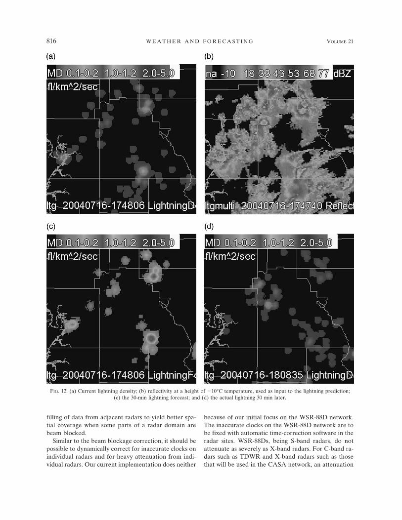
The assumptions for a beam being blocked veryclosely follow the techniques of O’Bannon (1997) andFulton et al. (1998). Interested readers should consultthose papers for further information. For each point inthe DEM, the azimuth, range, and elevation angle of athin radar beam are computed following the standardbeam propagation assumptions and tolerances as givenby O’Bannon (1997). Any thin beam above this eleva-tion angle passes above this terrain point unblocked.Other beams are assumed to be blocked by this eleva-tion point. Every radial from the radar is then consid-ered a numerical integrand of all the thin beams thatfall within its range of azimuths and elevations. Theinfluence of the individual thin beams follows thepower density function of Doviak and Zrnic (1993).Thus, a fraction of the beam that is blocked is known ateach range gate. If this fraction is greater than 0.5, theentire range gate is assumed to be blocked; the datafrom such range gates are not used to create new intel-ligent agents. However, because of advection, it is pos-sible that a voxel that would be beam blocked might geta value due to the movement of an agent created froma nonblocked range gate. Beam-blocked voxels can alsoget filled in by data from other nearby radars, leadingto a more uniform spatial coverage than what is pos-sible using just one radar. Figure 13 demonstrates the

FIG. 10. Multiradar VIL product at high spatial (approximately1 km � 1 km) and temporal (60-s update) resolution from thelatest reflectivity data from four radars: KFDR, KAMA, KLBB,and KFWS on 3 May 2003.

FIG. 11. The VDL computed on cells detected from datablended from individual radars is more robust than VIL computedon storms cells identified from a single radar. As the storm ap-proaches the radar, the single-radar VIL drops because higher-elevation data are unavailable. The multiradar product does nothave that problem. Image courtesy of Stumpf et al. (2004).


filling of data from adjacent radars to yield better spa-tial coverage when some parts of a radar domain arebeam blocked.

Similar to the beam blockage correction, it should bepossible to dynamically correct for inaccurate clocks onindividual radars and for heavy attenuation from indi-vidual radars. Our current implementation does neither

because of our initial focus on the WSR-88D network.The inaccurate clocks on the WSR-88D network are tobe fixed with automatic time-correction software in theradar sites. WSR-88Ds, being S-band radars, do notattenuate as severely as X-band radars. For C-band ra-dars such as TDWR and X-band radars such as thosethat will be used in the CASA network, an attenuation

FIG. 12. (a) Current lightning density; (b) reflectivity at a height of �10°C temperature, used as input to the lightning prediction;(c) the 30-min lightning forecast; and (d) the actual lightning 30 min later.


FIG. 13. (a) Vertical slice through data from the Phoenix, AZ (KIWA), radar on 14 Aug2004. (b) Elevation scan from the KIWA radar, note the extensive beam blockage. (c) Verticalslice through multiradar data from KIWA; Tucson, AZ (KEMX); Yuma, AZ (KYUX); Flag-staff, AZ (KFSX); and Albuquerque, NM (KABX) covering the same domain. (d) A 5-kmhorizontal slice through multiradar data. Note that the entire domain is filled in.


correction will have to be put in place to avoid an un-derreporting bias in the multiple-radar grids.

b. Quality control of input data

Weather radar data are subject to many contami-nants, mainly due to nonprecipitating targets (such asinsects and wind-borne particles) and anomalouspropagation (AP) or ground clutter. If the radar dataare directly placed into the 3D merged grid, these arti-facts lower the quality of the gridded data. Hence, theradar velocity data need to be dealiased and the radarreflectivity data need to be quality controlled. We used

the standard WSR-88D dealiasing algorithm to dealiasthe velocity data.

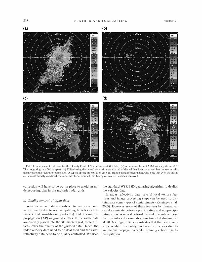
In radar reflectivity data, several local texture fea-tures and image processing steps can be used to dis-criminate some types of contaminants (Kessinger et al.2003). However, none of these features by themselvescan discriminate between precipitating and nonprecipi-tating areas. A neural network is used to combine thesefeatures into a discrimination function (Lakshmanan etal. 2003a). Figure 14 demonstrates that the neural net-work is able to identify, and remove, echoes due toanomalous propagation while retaining echoes due toprecipitation.

FIG. 14. Independent test cases for the Quality Control Neural Network (QCNN). (a) A data case from KAMA with significant AP.The range rings are 50 km apart. (b) Edited using the neural network; note that all of the AP has been removed, but the storm cellsnorthwest of the radar are retained. (c) A typical spring precipitation case. (d) Edited using the neural network; note that even the stormcell almost directly overhead the radar has been retained, but biological scatter has been removed.


No current technique using only single radar-data(ignoring polarimetric data) can discriminate betweenshallow precipitation and spatially smooth clear-air re-turns (Lakshmanan and Valente 2004). The radar-onlytechniques also have problems removing some biologi-cal targets, chaff, and terrain-induced ground clutter faraway from the radar. In addition to the radar-only qual-ity control above, an additional stage of multisensorquality control is applied. This uses satellite data andsurface temperature data to remove clear-air echoes.Figure 15 demonstrates that biological returns may beremoved by using such cloud cover information. Formore details, the reader is directed to Lakshmanan andValente (2004).

The radar reflectivity elevation scans are quality con-trolled, either using the radar-only quality control tech-nique described in Lakshmanan et al. (2003a) or usingthe multisensor technique described in Lakshmanan

and Valente (2004). It is these quality-controlled reflec-tivity data that are presented to the agent frameworkfor incorporation into the constantly updating grid.

c. Precomputation

The coordinate system transformation to go fromeach voxel �g, �g, hg to the spherical coordinate system(a, r, e) can be precomputed as long as we limit theinput radars to be nonmobile units (so that the radarposition does not change). If the radar follows one of aset number of VCPs, then the elevation scan can bedetermined from e. If the elevation scans are indexed toalways start at a specific azimuth and each beam con-strained to an exact beamwidth (WSR-88D scans arenot), then a, r can also be mapped to specific locationsin the radar array. In fact, the presence of a VCP is notrequired to precompute the effect of data from an el-evation angle; all that is required is that the radar op-

FIG. 15. (a) KTLX reflectivity composite showing the effects of biological contamination. (b) The cloud cover field derived fromsatellite data and surface observations. (c) The effect of the radar-only quality control neural network. (d) The effect of using both theradar-only neural network and the cloud cover field. Note that the small cells to the northwest of the radar are unaffected, but thebiological targets to the south of the radar are removed.


erate only at a limited number of elevation angles, per-haps in a range of [0°, 20°] in increments of 0.1°. Then,the voxels impacted by data from an elevation scan canbe computed beforehand and stored as part of the com-puter’s permanent memory (i.e., on the hard drive) forimmediate recall whenever that elevation angle fromthat radar is received. Intelligent agents can then becreated, with coordinates assigned to them in both co-ordinate systems at the time of creation. If the VCPsare known or if the radar operates only at set eleva-tions, it is possible to precompute the elevation weight�e. However, because of the dependence on t, a time-delay variable, it is necessary to compute � at the timeof grid creation. Similarly, the presence of t in the ad-vection equations necessitates that the movement ofthe agents to their new positions be dynamic and notprecomputed.

These precomputations have to be performed for ev-ery possible elevation angle from every radar that willbe used as an input to the merged 3D grid. For a grid ofapproximately 800 km � 800 km and about 10 radars, atypical regional domain, the precomputation can takeup to 8 h on a workstation with a 1.8-GHz Intel Xeonprocessor, 2 GB of random access memory, and a 512-MB cache (referred to from hereon as simply IntelXeon). Thus, it is necessary to decide upon a regionaldomain well in advance of the storm event, or to haveenough hardware available to process a large radar do-main reflecting the threat 6–8 h in advance.

d. Extraction of subdomains

Naturally, determining the domain of interest 6–8 hin advance is not a trivial task. Is it possible to reuseprecomputations? Because the coordinate system ofthe output 3D grid is a rectilinear system (the �g, �g, hg

are additive), we can precompute the transformation ofdata from any radar in the country at every elevationangle possible onto a domain the size of the entire con-tinental United States (CONUS). The CONUS domaincan be created at the desired resolution. We currentlyuse 0.01° in latitude and longitude and 1 km in height,approximately 1 km � 1 km � 1 km at midlatitudes.Then, the coordinates of the range gate in a subdomainof the CONUS domain can be computed from its co-ordinates in the CONUS domain using the offsets ofthe corners. If the northwest corner of the CONUSdomain is �c, �c, hc and that of the desired subdomainis �s, �s, hs, then the additive correction to the �g, �g, hg

entries in the CONUS cache to yield correct subdomainentries is

�� g � �c�res�

�� c � �g�res�, �12

where res�, res� are the resolution of the 3D grid in thelatitudinal and longitudinal directions. The only condi-tion is that the above operations have to yield integers,because they will be indexes into the CONUS domainarrays. Thus, the limitation is that subdomains have tobe defined at 0.01°/1-km increments. Computation ofthe CONUS domain takes about 120 h on a dual-processor workstation and requires 77 GB of diskspace. However, this needs to be done only once andcan be farmed out to a bank of such machines to reducethe computation time. With this precomputed CONUSdomain, we gain the ability to quickly switch domains.See Levit et al. (2004) for how this capability is used toget real-time access to merged 3D radar data from any-where in the country using a single workstation.

e. Time correction

Motion estimates obtained from the technique de-scribed in Lakshmanan et al. (2003b) are used to cor-rect for time differences between the sensing of thesame storms by different radars using Eq. (5). This dra-matically improves the value of derived products com-puted from the 3D grid because, by correcting the lo-cations of the storms, the areas sensed by different ra-dars line up in space and time. Figure 2 demonstratesthe significant difference between an uncorrected im-age and a time-corrected one.

The characteristics of the motion estimation tech-nique impact the results in the merged grid. If the mo-tion of a few storms is underestimated, then thosestorms will appear to jump whenever newer data areobtained, as the intelligent agents correct their posi-tions. Because the motion estimation technique of Lak-shmanan et al. (2003b) is biased toward estimating themovement of larger storms correctly, smaller cells andcells with erratic movements will tend to not providesmooth transitions. However, the transition in suchcases will typically still be less than the transition thatwould have resulted if no advection correction hadbeen applied.

Weighting individual observations by time [in addi-tion to distance; see Eq. (7)] can have undesirable sideeffects if the radars are not calibrated identically. If oneradar is “hotter” than all the others, then in those timeframes where data from that radar are the latest avail-able, the merged image will appear hotter. This prob-lem affects radar data from the WSR-88D network be-cause of large calibration differences between indi-vidual radars (Gourley et al. 2003) and is most evidentwhen viewing time sequences of merged radar data.

In the absence of time weighting, however, themerged data will be a biased estimate in areas wherethe storms are exhibiting fast variations in intensity be-


cause older data are still retained. The older data areadvected to their correct positions, but no compensa-tion is made for potential changes in intensity becausethe automated extraction of the growth/decay of thestorm was found to possess very little skill (Laksh-manan et al. 2003b). Therefore, calibration differencesstill remain evident when looking at features that mi-grate from the domain of one radar to the domain ofanother, especially when these features are accumu-lated over time.

One solution to the problem of combining timeweighting with calibration differences between radars isto retain time weighting but to apply calibration cor-rections to the data from individual radars. We intendto implement such a calibration correction in futureresearch.

f. Timing

The time taken to read individual elevation scans,update the 3D grid by creating intelligent agents, andwrite the current state of the 3D grid periodically de-pends on a variety of factors. We carried out a testwhere the individual elevation scans and the outputgrid are both compressed (as will be the case in a net-worked environment, to conserve bandwidth), so thatall of these timing data reflect the time taken to un-compress while reading and compress when writing.We carried out this test for a 650 � 700 � 18 regionaldomain with convective activity in most parts of theregion and using data from three WSR-88Ds. Differenttasks scale to either the domain size or the number ofradars. These are marked along with the timing infor-mation in Table 1. The test was carried out on theaforementioned Intel Xeon workstation.

Table 1 can be used to determine the computingpower needed for different domain sizes and numbersof radars. On average, we require 0.5 seconds per el-evation scan and 2.75 seconds per million voxels. Itshould be noted that merging radar data using the tech-nique described in this paper is an “embarrassingly par-

allel” problem; that is, if multiple machines are put towork on the problem, each machine can concentrate ona subdomain and the output grids can be cheaplystitched together again. The subdomains do have topartially overlap to take into account advection effects.

Using the information in Table 1, we can estimate thecomputational requirements necessary to create a 5000� 3000 � 20 domain every 60 s in real time using in-formation from 130 WSR-88Ds. Let us estimate that wewill receive a new elevation scan from each of the ra-dars every 30 s (in areas having significant weather, thiswill be around 20 s while in areas of little weather, theinterval approaches 120 s). Thus, we will have 260 el-evation scans per minute to read and update, which willtake about 130 wall-clock seconds on our single work-station. Because our 5000 � 3000 � 20 domain contains300 million voxels, creating and writing out the grid willtake 1125 more seconds. Our single workstation, if out-fitted with enough computer memory, will be able tocreate and write 3D merger grids for this domain in1250 s. To maintain our update interval of 60 s, wewould require about 20 such workstations. The hard-ware requirements for several scenarios are provided inTable 2. Levit et al. (2004) used the regional configu-ration in their study.

5. Summary

In this paper, we have described a technique basedon an intelligent agent formulation for taking the baseradar data (reflectivity and radial velocity), and derivedproducts, from multiple radars and combining them inreal time into a rapidly updating 3D merged grid. Wedemonstrated that the intelligent formulation accountsfor the varying radar beam geometry with range, verti-cal gaps between radar scans, the lack of time synchro-nization between radars, storm movement, varyingbeam resolutions between different types of radars,beam blockage due to terrain, differing radar calibra-tion, and inaccurate time stamps on radar data.

The techniques described in this paper of mergingmoment data from individual radars have been testedin real time and on archived data cases in diverse stormregimes. They have been tested on different types ofradars as well. For example, Fig. 3 shows the techniqueoperating in a hurricane event. Figure 13 shows thetechnique operating on late-summer monsoon events inan area with terrain. Figures 2, 9, and 10 illustrate theuse of this technique in convective situations, while Fig.5 illustrates a stratiform one. One of the radars in Fig.6 is a TDWR while the others are WSR-88Ds, whileFig. 7 shows simulated CASA radars.

With the continuing improvements in computer pro-

TABLE 1. Timing statistics collected in real time for readingradar data and creating 3D merged grids of reflectivity.

Aspect CPU time (s) Clock time (s) Scaling

Read radarscan

0.012 � 0.001 0.254 � 0.023 One elevationscan

Update gridwith scan

0.075 � 0.007 1.28 � 0.135 One elevationscan

Create 3Dgrid

0.594 � 0.127 9.179 � 2.056 8-m voxels

Write 3Dgrid

1.257 � 0.268 20.68 � 4.62 8-m voxels


cessors, operating systems, and input–output perfor-mance, preliminary tests indicate that a 2-min CONUS3D merger can be implemented using a single 3-GHz64-bit processor with 8 GB of RAM. Thus, we plan tostart utilizing this technique to merge scalar fields, bothreflectivity and derived shear products, from all theWSR-88D radars in the continental United States. Wenow have the ability to ship the merged products in realtime to Advanced Weather Interactive Processing Sys-tem (AWIPS) and National Centers for EnvironmentalPrediction AWIPS (N-AWIPS) workstations atweather forecast offices and national centers. Becausethese workstations will be unable to handle the data atits highest resolution and spatial extent, we may have tosubsect the data before shipping it to operational cen-ters. The merged products created using the techniquedescribed in this paper are now available in real time(online at http://wdssw.nssl.noaa.gov/).

Also note that the software implementing this tech-nique of combining data from multiple radars is freelyavailable online (at http://www.wdssii.org/) for researchand academic use.

Acknowledgments. Funding for this research wasprovided under NOAA–OU Cooperative AgreementNA17RJ1227, National Science Foundation GrantsITR 0205628 and 0313747, and the National SevereStorms Laboratory. Part of the work was performed incollaboration with the CASA NSF Engineering Re-search Center (EEC-0313747). We thank Kiel Ortegafor creating some of our data cases, Jian Zhang for heruseful pointers at several stages of this research,Rodger Brown for guidance on the multi-Doppler ve-locity combination approach and the anonymous re-viewers whose inputs improved the clarity of our paper.The statements, findings, conclusions, and recommen-dations are those of the authors and do not necessarilyreflect the views of the National Severe Storms Labo-ratory, the National Science Foundation, or the U.S.Department of Commerce.

REFERENCES

Adrianto, I., T. M. Smith, K. A. Scharfenberg, and T. Trafalis,2005: Evaluation of various algorithms and display concepts

for weather forecasting. Preprints, 21st Int. Conf. on Interac-tive Information Processing Systems for Meteorology, Ocean-ography, and Hydrology, San Diego, CA, Amer. Meteor.Soc., CD-ROM, 5.7.

Askelson, M., J. Aubagnac, and J. Straka, 2000: An adaptation ofthe Barnes filter applied to the objective analysis of radardata. Mon. Wea. Rev., 128, 3050–3082.

Beyer, W., Ed., 1987: CRC Standard Math Tables. 18th ed. CRCPress, 487 pp.

Biggerstaff, M. I., and R. M. May, 2005: A meteorological radaremulator for education and research. Preprints, 21st Int.Conf. on Interactive Information Processing Systems for Me-teorology, Oceanography, and Hydrology, San Diego, CA,Amer. Meteor. Soc., CD-ROM, 5.6.

Brotzge, J., D. Westbrook, K. Brewster, K. Hondl, and M. Zink,2005: The meteorological command and control structure ofa dynamic, collaborative, automated radar network. Pre-prints, 21st Int. Conf. on Interactive Information ProcessingSystems for Meteorology, Oceanography, and Hydrology, SanDiego, CA, Amer. Meteor. Soc., CD-ROM, 19.15.

Brown, R., and P. Hwang, 1997: Introduction to Random Signalsand Applied Kalman Filtering. John Wiley and Sons, 480 pp.

Browning, K., and A. Wexler, 1968: The determination of kine-matic properties of a wind field using Doppler radar. J. Appl.Meteor., 7, 105–113.

Burrows, M., and D. Wheeler, 1994: A block-sorting lossless datacompression algorithm. Digital Equipment CorporationTech. Rep. 124, Palo Alto, CA, 18 pp. [Available online atgatekeeper.dec.com/pub/DEC/SRC/research-reports/abstracts/src-rr-124.html.]

Charba, J., and F. Liang, 2005: Quality control of gridded nationalradar reflectivity data. Preprints, 21st Conf. on WeatherAnalysis and Forecasting/17th Conf. on Numerical WeatherPrediction, Washington, DC, Amer. Meteor. Soc., CD-ROM,6A.5.

Doviak, R., and D. Zrnic, 1993: Doppler Radar and Weather Ob-servations. 2d ed. Academic Press, 458 pp.

Droegemeier, K., and Coauthors, 2002: Project CRAFT: A testbed for demonstrating the real time acquisition and archivalof WSR-88D level II data. Preprints, 18th Int. Conf. on In-teractive Information Processing Systems for Meteorology,Oceanography, and Hydrology, Orlando, FL, Amer. Meteor.Soc., 136–139.

Foote, G., and P. S. duToit, 1969: Terminal velocity of raindropsaloft. J. Appl. Meteor., 8, 249–253.

Fulton, R., D. Breidenback, D. Miller, and T. O’Bannon, 1998:The WSR-88D rainfall algorithm. Wea. Forecasting, 13, 377–395.

Gourley, J. J., B. Kaney, and R. A. Maddox, 2003: Evaluating thecalibrations of radars: A software approach. Preprints, 31stInt. Conf. on Radar Meteorology, Hyannis, MA, Amer. Me-teor. Soc., CD-ROM, P3C.1.

TABLE 2. Estimated hardware requirements for implementing this technique. The machine referred to here is a 1.8-GHz Intel Xeonprocessor with 2 GB of RAM.

Update interval Domain size No. of radars Domain resolution No. of machines

CONUS 1 min 5000 km � 3000 km � 20 km 130 1 km � 1 km � 1 km 20Regional 1 min 800 km � 800 km � 20 km 10 1 km � 1 km � 1 km 1CONUS 5 min 5000 km � 3000 km � 20 km 130 1 km � 1 km � 1 km 4


Greene, D. R., and R. A. Clark, 1972: Vertically integrated liquidwater—A new analysis tool. Mon. Wea. Rev., 100, 548–552.

Johnson, J., P. MacKeen, A. Witt, E. Mitchell, G. Stumpf, M.Eilts, and K. Thomas, 1998: The Storm Cell Identificationand Tracking Algorithm: An enhanced WSR-88D algorithm.Wea. Forecasting, 13, 263–276.

Kalman, R., 1960: A new approach to linear filtering and predic-tion problems. Trans. ASME J. Basic Eng., 82D, 35–45.

Kessinger, C. J., P. Ray, and C. E. Hane, 1987: The Oklahomasquall line of 19 May 1977. Part I: A multiple Doppler analy-sis of convective and stratiform structure. J. Atmos. Sci., 44,2840–2864.

——, S. Ellis, and J. Van Andel, 2003: The radar echo classifier: Afuzzy logic algorithm for the WSR-88D. Preprints, ThirdConf. on Artificial Applications to the Environmental Sci-ences, Long Beach, CA, Amer. Meteor. Soc., CD-ROM, P1.6.

Lakshmanan, V., and M. Valente, 2004: Quality control of radarreflectivity data using satellite data and surface observations.Preprints, 20th Int. Conf. on Interactive Information Process-ing Systems for Meteorology, Oceanography, and Hydrology,Seattle, WA, Amer. Meteor. Soc., CD-ROM, 12.2.

——, K. Hondl, G. Stumpf, and T. Smith, 2003a: Quality controlof weather radar data using texture features and a neuralnetwork. Fifth Int. Conf. on Advances in Pattern Recognition,Calcutta, India, IEEE–Indian Statistical Institute, 54–59.

——, R. Rabin, and V. DeBrunner, 2003b: Multiscale storm iden-tification and forecast. Atmos. Res., 67/68, 367–380.

Levit, J. J., V. Lakshmanan, K. L. Manross, and R. Schneider,2004: Integration of the Warning Decision Support System-Integrated Information (WDSS-II) into the NOAA StormPrediction Center. Preprints, 22d Conf. on Severe LocalStorms, Hyannis, MA, Amer. Meteor. Soc., CD-ROM, 8B4.

Lhermitte, R., and D. Atlas, 1961: Precipitation motion by pulseDoppler. Preprints, Ninth Conf. on Radar Meteorology, Bos-ton, MA, Amer. Meteor. Soc., 218–223.

Liou, Y.-C., 2002: An explanation of the wind speed underesti-mation obtained from a least squares type single-Dopplerradar velocity retrieval method. J. Appl. Meteor., 41, 811–823.

Maes, P., 1995: Artificial life meets entertainment: Life-like au-tonomous agents. Commun. ACM, 38, 108–114.

McNellis, T., S. Katz, M. Campbell, and J. Melody, 2005: Recentadvances in phased array radar for meteorological applica-tions. Preprints, 21st Int. Conf. on Interactive Information

Processing Systems for Meteorology, Oceanography, and Hy-drology, San Diego, CA, Amer. Meteor. Soc., CD-ROM,19.6.

O’Bannon, T., 1997: Using a terrain-based hybrid scan to improveWSR-88D precipitation estimates. Preprints, 28th Conf. onRadar Meteorology, Austin, TX, Amer. Meteor. Soc., 506–507.

Rabin, R., and D. Zrnic, 1980: Subsynoptic-scale vertical windrevealed by dual Doppler-radar and VAD analysis. J. Atmos.Sci., 37, 644–654.

Smith, D. C., A. Cypher, and J. Spohrer, 1994: KidSim: Program-ming agents without a programming language. Commun.ACM, 37, 55–67.

Smith, T. M., and K. L. Elmore, 2004: The use of radial velocityderivatives to diagnose rotation and divergence. Preprints,11th Conf. on Aviation, Range, and Aerospace, Hyannis, MA,Amer. Meteor. Soc., CD-ROM, P5.6.

Stumpf, G. J., T. M. Smith, and J. Hocker, 2004: New hail diag-nostic parameters derived by integrating multiple radars andmultiple sensors. Preprints, 22d Conf. on Severe LocalStorms, Hyannis, MA, Amer. Meteor. Soc., CD-ROM, P7.8.

——, S. Smith, and K. Kelleher, 2005: Collaborative activities ofthe NWS MDL and NSSL to improve and develop new mul-tiple-sensor severe weather warning guidance applications.Preprints, 21st Int. Conf. on Interactive Information Process-ing Systems for Meteorology, Oceanography, and Hydrology,San Diego, CA, Amer. Meteor. Soc., CD-ROM, P2.13.

Trapp, R. J., and C. A. Doswell, 2000: Radar data objective analy-sis. J. Atmos. Oceanic Technol., 17, 105–120.

Witt, A., M. Eilts, G. Stumpf, J. Johnson, E. Mitchell, and K.Thomas, 1998: An enhanced hail detection algorithm for theWSR-88D. Wea. Forecasting, 13, 286–303.

——, R. A. Brown, and V. Lakshmanan, 2005: Real-time calcu-lation of horizontal winds using multiple Doppler radars: Anew WDSS-II module. Preprints, 32d Conf. on Radar Meteo-rology, Albuquerque, NM, Amer. Meteor. Soc., CD-ROM,P8R7.

Zhang, J., K. Howard, and J. J. Gourley, 2005: Constructing three-dimensional multiple-radar reflectivity mosaics: Examples ofconvective storms and stratiform rain echoes. J. Atmos. Oce-anic Technol., 22, 30–42.


Date post:	09-Jun-2018
Category:	Documents
Upload:	vutuyen
View:	215 times
Download:	0 times

A Real-Time, Three-Dimensional, Rapidly Updating ...€¦ · A Real-Time, Three-Dimensional,...

Documents