A RECONSTRUCTION ALGORITHM FOR ULTRASOUND …algorithm for ultrasound-modulated diﬀuse optical...

A RECONSTRUCTION ALGORITHM FOR

ULTRASOUND-MODULATED DIFFUSE OPTICAL

TOMOGRAPHY

HABIB AMMARI, EMMANUEL BOSSY, JOSSELIN GARNIER, LOC HOANG NGUYEN,

AND LAURENT SEPPECHER

Abstract. The aim of this paper is to develop an efficient reconstruction

algorithm for ultrasound-modulated diffuse optical tomography. In diffuse op-

tical imaging, the resolution is in general low. By mechanically perturbing themedium, we show that it is possible to achieve a significant resolution enhance-

ment. When a spherical acoustic wave is propagating inside the medium, the

optical parameter of the medium is perturbed. Using cross-correlations of the

boundary measurements of the intensity of the light propagating in the per-turbed medium and in the unperturbed one, we provide an iterative algorithm

for reconstructing the optical absorption coefficient. Using a spherical Radontransform inversion, we first establish an equation that the optical absorption

satisfies. This equation together with the diffusion model constitutes a non-linear system. Then, solving iteratively such a nonlinear coupled system, weobtain the true absorption parameter. We prove the convergence of the al-

gorithm and present numerical results to illustrate its resolution and stabilityperformances.

1. Introduction

Diffuse optical tomography is an emerging biomedical modality that uses dif-fuse light to probe structural variations in the optical properties of tissue [6]. Theassociated inverse problem for diffuse waves consists of recovering the absorptionproperties of a medium of interest from boundary measurements of the light in-tensity. The most important current applications of diffuse optical imaging aredetecting tumors in the breast and brain imaging [8].

Let Ω be a smooth bounded domain of Rd, for d = 2, 3, satisfying the interior ball

condition. The aim of this paper is to reconstruct the optical absorption coefficientq∗ of a medium occupied by Ω under the Born assumption that q takes the form

(1.1) q∗ = q0(1 + δs∗).

Here δ is a small constant and s∗ is a smooth function whose supportD is known andcompactly contained in the background medium Ω. The Born approximation and itshigher order corrections have been widely used; see, for instance, [14, 15, 21, 16, 22].

In optical tomography, the diffusion equation can be used in biomedical appli-cations to describe the propagation of light. The diffusion equation holds when the

2000 Mathematics Subject Classification. 65R32, 44A12, 31B20.Key words and phrases. Ultrasound-modulated optical imaging, diffuse optical tomography,

spherical Radon transform, Helmholtz decomposition, reconstruction, convergence.This work was supported by the ERC Advanced Grant Project MULTIMOD–267184.

1

2 ULTRASOUND-MODULATED DIFFUSE OPTICAL TOMOGRAPHY

scattering coefficient is large, the absorption coefficient is small, the point of ob-servation is far from the boundary of the medium and the time-scale is sufficientlylong [25, 26]. Under these assumptions, using boundary measurements of the lightintensity, that is the normal derivative of the solution to the diffusion equation,it is possible to determine the optical coefficient q∗ [6, 26]. Direct reconstructionmethods have been designed in the linearized case under consideration for partic-ular experimental geometries [26]. However, the resolution of the reconstructionis usually low due to the inherent severely ill-posed character of diffuse opticalimaging.

In this paper we propose a new method for reconstructing the optical coefficientby using mechanical perturbations of the medium. While taking optical measure-ments we perturb the medium by a propagating acoustic wave. Then we computethe cross-correlations between the boundary values of the intensity of the light prop-agating in the medium changed by the propagation of the acoustic wave and thosecorresponding to the unperturbed one. The use of a spherical Radon transforminversion will yield an equation for q∗ and hence a coupled system. The obtainednonlinear coupling suggests an iterative algorithm under the Born assumption. Weprove convergence of the iterative algorithm to the true image of q∗ using the con-traction fixed point theorem.

The idea of mechanically perturbing the medium has been first introduced in [3]for electromagnetic imaging. In [3], since the amplitude of the background solutionis constant an inversion of the spherical Radon transform yields the correct image.The algorithm proposed in [3] is a direct algorithm. On the other hand, it is alsoworth emphasizing that this approach is different from the imaging by controlledperturbations [1, 2, 10, 5], where local changes of the parameters of the mediumare produced by focalizing an ultrasound beam. Both techniques lead to resolutionenhancements. In imaging by controlled perturbations, the resolution is of orderthe size of the focal spot while here it is of order the width of the wave front of thewave propagating in the medium. Our new method is called ultrasound-modulatedoptical tomography. It significantly differs from those proposed in [9, 11, 28], wherethe spatial scales are much smaller than those considered here. The model underconsideration in this paper corresponds to the macroscopic case while the one for[9, 11, 28] refers to the microscopic case. In [7], an ultrasound-modulated approachfor diffuse optical imaging has been proposed. However, the modulation of themedium is different. For the acoustic wave, plane waves are used in [7] insteadof spherical waves here. This leads to a completely different model: a nonlinearpartial differential equation (called zero-Laplacian) for the energy density. Whilethe algorithms developed in [2, 10] can be used to efficiently solve such a nonlinearPDE, new techniques have to be designed for the present spherically modulatedmodel.

The paper is organized as follows. In Section 2, we introduce some preliminaryresults. In Section 3, we present our reconstruction algorithm. In Section 4 weprovide a proof of convergence of the algorithm. In Section 5 we illustrate theperformance of the proposed algorithm in terms of resolution and stability. Thepaper ends with a short discussion. Throughout the paper, ν denotes the unitnormal outward vector on ∂Ω, ∂ν denotes the normal derivative at ∂Ω, and C is anuniversal constant depending only on known quantities and functions.

ULTRASOUND-MODULATED DIFFUSE OPTICAL TOMOGRAPHY 3

2. Preliminaries

In this section, we first recall two consequences of well-known regularity results.The propositions we present here are special cases in those papers and enough forus to study ultrasound-modulated optical tomography. The reader can find thefollowing result in [17, 19].

Proposition 2.1. Suppose that Ω is smooth. If p ∈ L∞(Ω), then any weak andbounded solution ϕ of the equation

(2.1) −∆ϕ+ pϕ = 0, with ‖ϕ‖L∞(Ω) ≤M,

is in C1(Ω) and

‖ϕ‖C1(Ω′

) ≤ c1(M, ‖p‖L∞(Ω),dist(Ω′, ∂Ω))

for all Ω′b Ω.

The following proposition is from [12, 18].

Proposition 2.2. Let D be a bounded smooth domain and λ < Λ,M be positiveconstants. If ϕ ∈ L∞(D) is such that

0 < λ ≤ ϕ ≤ Λ in D

and if f ∈ L∞(D) is such that ‖f‖L∞(D) ≤M , then the solution q of

(2.2)

∇ · (ϕ2∇q) = f in D,q = 0 on ∂D

is in C1(D) with

(2.3) ‖q‖C1(D) ≤ c2(λ,Λ,M).

Remark 2.3. Assume that the constant c2 in (2.3) is optimal; i.e., c2 is the infimumof all of its possible values. Then,

(2.4) c2(λ,Λ, δM) ≤ δc2(λ,Λ,M)

for all 0 < δ < 1. This can be seen by multiplying both sides of (2.2) by δ.

We next establish the weak comparison principle and the strong maximum prin-ciple for Laplace equations with the Robin boundary condition under consideration.The main idea of the proof is based on the weak comparison principle in [20] forDirichlet boundary conditions, with some suitable modifications. Although thismight be a well-known result, we provide a proof here for the sake of completeness.Also, our strong maximum principle is somewhat different from the classical one.

Proposition 2.4 (weak comparison principle). Let p be a nonnegative measurablefunction and assume that ϕ ∈ H1(Ω) satisfies

(2.5)

−∆ϕ+ pϕ ≥ 0 in Ω,∂νϕ+ ϕ ≥ 0 on ∂Ω.

We have ϕ ≥ 0 a.e. in Ω.


Proof. Using ϕ− = max0,−ϕ ≥ 0 as a test function in the variational formulationof (2.5) gives

0 ≤

∫

Ω

∇ϕ∇ϕ−dx −

∫

∂Ω

∂νϕϕ−dσ +

∫

Ω

pϕϕ−dx

≤

∫

Ω

∇ϕ∇ϕ−dx +

∫

∂Ω

ϕϕ−dσ +

∫

Ω

pϕϕ−dx

= −

∫

Ω

|∇ϕ−|2dx −

∫

∂Ω

|ϕ−|2dσ −

∫

Ω

p|ϕ−|2dx.

It follows that ϕ− = 0. Note that ϕ− is admissible to be a test function because itbelongs to H1(Ω) (see [13]).

Proposition 2.5 (strong maximum principle). Let g 6≡ 0 be a nonnegative smoothfunction defined on ∂Ω. Let D b Ω be smooth. For all c > 0, the solution ϕc of

(2.6)

−∆ϕc + cϕc = 0 in Ω,∂νϕc + ϕc = g on ∂Ω,

is bounded and positive in D.

We need the following lemma to prove this strong maximum principle [23].

Lemma 2.6 (Hopf lemma). Let ϕ ∈ C1(

Ω)

∩ C2 (Ω) satisfy

−∆ϕ+ cϕ ≥ 0

on Ω where c is a nonnegative constant. If there exists x0 ∈ ∂Ω such that ϕ(x0) ≤ 0and ϕ(x) > ϕ(x0) for all x ∈ Ω, then

∂νϕ(x0) < 0.

Proof of Proposition 2.5. Since g is nonnegative, so is ϕc because of Proposition2.4. On the other hand, applying Proposition 2.4 again for ‖g‖L∞(∂Ω) − ϕ, wecan see that ϕ ≤ ‖g‖L∞(∂Ω). The boundedness of ϕc in Ω and hence D has been

verified. In order to use the Hopf lemma, we show that ϕc ∈ C2(Ω). In fact, for allx0 ∈ Ω, let D1 and D2 satisfying

D1 b D2 b Ω

be two open neighbourhoods of x0. The boundedness of ϕc in the previous para-graph and Proposition 2.1 imply ϕc belongs to C1(D2). On the other hand, Theo-rem 8.8 in [13] helps us to see that ϕc ∈ H2(D2). Hence, ∂xi

ϕc, i = 1, · · · , d, is inH1(D2). It also satisfies the equation

−∆∂xiϕc + c∂xi

ϕc = 0.

Hence, ∂xiϕc belongs to C1(D1) by Proposition 2.1. In other words, ϕc ∈ C2(D1).

We claim that ϕc > 0 not only in D but also in Ω. Assume that ϕc(x0) = 0for some x0 ∈ Ω. Since g is not identically zero, so is ϕc. Hence, we can find apoint x1 ∈ Ω such that ϕc(x1) > 0. Without loss of generality, we can supposethat B(x1, r) ⊂ Ω with r = |x1 − x0| and ϕc(x) > 0 for all x ∈ B(x1, r). Since

ϕc ∈ C2(Ω), it belongs to C1(B(x1, r)) ∩ C2(B(x1, r)). We can apply the Hopflemma for ϕc in B(x1, r) to get

∇ϕc(x0) · (x1 − x0) < 0.

This is a contradiction because ϕc attains its minimum value at x0 and ∇ϕc(x0) =0.


3. A reconstruction algorithm

When a laser beam is applied at a point x0 on ∂Ω, the energy density ϕ∗ isgoverned by the problem

(3.1)

−∆ϕ∗ + q∗ϕ∗ = 0 in Ω,l∂νϕ∗ + ϕ∗ = g on ∂Ω,

where q∗ is the (spatially-varying) optical absorption coefficient and g ≥ 0 is asmooth approximation of the Dirac function at x0. Note that in the Robin typeboundary condition in (3.1), l is the extrapolation length [24]. From now on wewill assume without loss of generality that l = 1. Note also that because of theexponential decay of ϕ∗, the inverse problem of finding q∗ from ∂νϕ∗ on ∂Ω isseverely ill-posed and the resolution of the reconstructed image is unsatisfactory[6, 26].

In order to achieve a resolution enhancement ultrasound-modulated optical to-mography can be used. Its basic principles are as follows. We generate a sphericalacoustic wave inside the medium. The propagation of the acoustic wave changesthe absorption parameter of the medium. During the propagation of the wave wemeasure the light intensity on ∂Ω. The aim is now to reconstruct the optical ab-sorption coefficient from such set of measurements with a better resolution andstability than using pure optical tomography.

In [3], we have shown that the displacement function u caused by a short diverg-ing spherical acoustic wave is of the form

(3.2) u(x) = uy(x, t) = −η

ctw

(

|x − y| − ct

η

)

x − y

|x − y|, x ∈ Ω,

where the constant c is the acoustic wave speed, y ∈ Rd \D is the position of the

acoustic wave generator, w ∈ C∞(R,R+), whose support is contained in [−1, 1], isthe shape function, η is a positive parameter representing the thickness of the wave-front, and t is understood as the time parameter. The support of the displacementfield u can be seen as a thin spherical shell growing at a constant speed c.

Denoting q∗(x + uy(x, t)) by qu(x,y, t), x ∈ Ω, y ∈ Ω \ D, t > 0, and thecorresponding energy density by ϕu(x,y, t), we have

(3.3)

−∆ϕu + quϕu = 0 in Ω,∂νϕu + ϕu = g on ∂Ω.

It follows from (3.1) and (3.3) that

‖ϕu − ϕ∗‖H1(Ω) ≤ c‖qu − q∗‖L2(Ω),

for some positive constant c, and therefore [3],

(3.4)

∫

∂Ω

g(∂νϕ∗ − ∂νϕu) dσ =

∫

Ω

ϕ∗ϕu(q∗ − qu) dx ≈ −

∫

Ω

ϕ2∗∇q∗ · u dx.

Since ∂νϕ∗ and ∂νϕu can be measured on ∂Ω, it is possible to evaluate thequantity

∫

∂Ωg(∂νϕ∗ − ∂νϕu) dσ for all y, t. This quantity is nothing else than

the cross-correlations between the boundary measurements in the perturbed andunperturbed media.

Next, from (3.4) we establish an equation for q∗. Using Helmholtz decomposition,we write

(3.5) ϕ2∗∇q∗ = −∇ψ + ∇× Ψ.


Here, in order to insure the uniqueness of ψ and Ψ we assume that Ω is simplyconnected, Ψ is such that ∇ · Ψ = 0, and supply the boundary conditions ∂νψ =−ϕ2

∗∂νq∗ and Ψ × ν = 0 on ∂Ω.Since u takes the radial form (3.2), integration by parts yields

∫

Ω

∇× Ψ · u dx = 0,

and so, (3.4) can be rewritten as∫

∂Ω

g(∂νϕ∗ − ∂νϕu) dσ ≈

∫

Ω

∇ψ · u dx.

Hence, ψ can be constructed and considered as the given data by employing thespherical Radon transform, as done in Section 5 in [3].

Let

(3.6) Nu(y, r) :=

∫

∂Ω

g(x)(

∂νϕ∗(x) − ∂νϕu(x,y, r/c))

dσ(x),

where uy is given by (3.2).For f ∈ C0(Rd) and E ⊂ R

d, define the spherical Radon transform of f over Eby

Rf(y, r) =1

|S|

∫

S

f(y + rξ) dσ(ξ) y ∈ E, r > 0,

where |S| is the surface of the unit sphere S and dσ is the surface measure over S.From [3] the following lemma holds.

Lemma 3.1. Fix y ∈ Ω \ D and let r0 > 0. Suppose that q∗(x) = q0 for x ∈B(y, r0), where B is the ball of center y and radius r0. Suppose also that q∗ ∈C1,β(Ω) and η is small enough. Then, for all r > r0 and η r, we have

Rψ(y, r) ≈ −1

η2‖w‖L1 |S|

∫ r

r0

Nu(y, ρ)

ρd−2dρ.

Having in hand ψ from the cross-correlations between boundary measurementsusing a spherical Radon transform inversion, we take the divergence of (3.5) toarrive at

−∇ · (ϕ2∗∇q∗) = ∆ψ.

This together with (1.1) also implies that

−∆ψ = δq0∇ · (ϕ2∗∇s∗),

where δ and s∗ were introduced in (1.1). Assume that q∗ is bounded from belowand above by two known positive constants q and q respectively. Since ϕ∗ solvesproblem (2.1) with q∗ replacing p and Λ, which will be defined later in Lemma 4.1,replacing M , its C1(D) norm is bounded. We assume further that δ is small ands∗ is smooth, with known bound on its C2(D) norm, to guarantee that ‖∆ψ‖L∞(D)

is bounded in the order of δ. The analysis allows us to recover q∗ in D by solvingthe system of equations for the two unknowns ϕ and q

(3.7)

−∆ϕ+ qϕ = 0 in Ω,∂νϕ+ ϕ = g on ∂Ω,

and

(3.8)

−∇ · (ϕ2∇q) = ∆ψ in D,q = q0 on ∂D,


where|∆ψ|L∞(Ω) = O(δ) as δ 1.

This suggests the following algorithm:

(1) Define the initial guess q(0) = q0.(2) Establish an iterating sequence q(n) as follows.

(a) For n ≥ 1, solve

(3.9)

−∆ϕ(n) + q(n−1)ϕ(n) = 0 in Ω,∂νϕ

(n) + ϕ(n) = g on ∂Ω,

wherep := minmaxp, q, q.

(b) Find q(n) by solving

(3.10)

−∇ · ((ϕ(n))2∇q(n)) = ∆ψ in D,q(n) = q0 on ∂D.

and defining q(n) = q0 in Ω \D.(3) The convergent function of q(n) is the true optical absorption coefficient

q∗.

Remark 3.2. The convergence of q(n), mentioned in step 3, will be shown by theBanach fixed point theorem in the next section. This also implies the well-posednessof the system constituted by (3.7) and (3.8).

Remark 3.3. Problem (3.9) is uniquely solvable because we are able to avoid thecase that (ϕ(n))2 approaches 0 or ∞ somewhere inside D in the next section (seeLemma 4.1).

Remark 3.4. We modify q(n−1) by q(n−1) in (3.9) because of the obvious inequality

|p− q∗| ≤ |p− q∗|,

which makes the proof of the algorithm easier and may increase the rate of conver-gence.

4. The convergence of the iterative algorithm

Define the open set of L∞(Ω)

(4.1) Q = p ∈ L∞(Ω) : q < p < q,

and the map

(4.2)F1 : Q → H1(Ω)

q 7→ F1[q] = ϕ,where ϕ is the solution of (3.7).

We have the following result.

Lemma 4.1. For all q ∈ Q, F1[q] is in L∞(Ω). There exists a positive constantΛ(q, q) such that

(4.3)∣

∣F1[q](x)∣

∣ ≤ Λ, ∀x ∈ Ω.

Moreover, for any D b Ω, there exists a positive constant λ(D, q, q) such that

(4.4) λ ≤ F1[q](x), ∀x ∈ D.


Proof. Let ϕq and ϕq be the solutions of (2.6) with c replaced by q and q, respec-

tively. It follows by Proposition 2.4 that

ϕq ≤ ϕ ≤ ϕq in Ω.

On the other hand, we can apply Proposition 2.5 to see that

ϕq > 0 in D.

The lemma is proved by letting λ = infD ϕq and Λ = supΩ ϕq.

Lemma 4.2. The map F1 is Frechet differentiable. Its derivative at q is given by

(4.5) DF1[q](h) = φ,

for h ∈ L∞(Ω), where φ solves

(4.6)

−∆φ+ qφ = −hϕ in Ω,∂νφ+ φ = 0 on ∂Ω,

with ϕ = F1[q]. Moreover, DF1[q] can be continuously extended to the whole L2(Ω)by the same formula in (4.6) with

(4.7) ‖DF1[q]‖L(L2(Ω),H1(Ω)) ≤ CΛ,

where Λ was defined in Lemma 4.1.

Proof. Let ϕ′ be the solution of (3.7) with q+h replacing q, assuming ‖h‖L∞(Ω) 1so that q + h ∈ Q a.e. in Ω. Note that ϕ′ − ϕ solves

−∆(ϕ′ − ϕ) + (q + h)(ϕ′ − ϕ) = −hϕ in Ω,∂ν(ϕ′ − ϕ) + (ϕ′ − ϕ) = 0 on ∂Ω.

Using ϕ′ −ϕ as a test function in the variational formulation of the problem abovegives

(4.8) ‖ϕ′ − ϕ‖H1(Ω) ≤ C‖h‖L∞(Ω)‖ϕ‖L2(Ω).

On the other hand, since ϕ′ − ϕ− φ solves

−∆(ϕ′ − ϕ− φ) + q(ϕ′ − ϕ− φ) = −h(ϕ′ − ϕ) in Ω,∂ν(ϕ′ − ϕ− φ) + (ϕ′ − ϕ− φ) = 0 on ∂Ω,

we can apply the argument above to obtain

(4.9) ‖ϕ′ − ϕ− φ‖H1(Ω) ≤ C‖h‖L∞(Ω)‖ϕ′ − ϕ‖L2(Ω).

Combining (4.8) and (4.9) shows that

‖ϕ′ − ϕ− φ‖H1(Ω) ≤ C‖h‖2L∞(Ω)‖ϕ‖L2(Ω),

which implies

lim‖h‖L∞(Ω)→0

‖ϕ′ − ϕ− φ‖H1(Ω)

‖h‖L∞(Ω)= 0.

The first part of the lemma follows.Because of Lemma 4.1 and Proposition 2.4, which shows that ϕ ∈ L∞(Ω),

problem (4.6) is uniquely solvable for all h ∈ L2(Ω) and therefore the extensionDF1[q] : L2(Ω) → H1(Ω) is well-defined. Its continuity and (4.7) can be deduced,using φ as a test function in the variational formulation of (4.6) and applyingLemma 4.1:

‖φ‖H1(Ω) ≤ C‖h‖L2(Ω)‖ϕ‖L∞(Ω).


We next introduce another open set of L∞(Ω)

(4.10) P =

ρ ∈ L∞(Ω) :λ

2< ρ < 2Λ in D

.

Let

F2 : P → H1(Ω)

ϕ 7→ F2[ϕ] = q, where q is the solution of (3.8) in D and q = q0 on Ω \D.

The following lemma can be proved in the same manner as Lemma 4.2.

Lemma 4.3. The map F2 is Frechet differentiable. Its derivative at ϕ is given by

(4.11) DF2[ϕ](h) = Q,

for h ∈ L∞(Ω), where Q solves

(4.12)

−∇ · (ϕ2∇Q) = ∇ · (2ϕh∇q) in D,Q = 0 on ∂D,

with q = F2[ϕ] being the solution of (3.8) and Q = 0 in Ω \D. Moreover, DF2[ϕ]can be extended continuously to L2(Ω) and

(4.13) ‖DF2[ϕ]‖L(L2(Ω),H1(Ω)) ≤2δΛq0λ2

c2(λ,Λ,M),

where M is an upper bound of ‖∇ · (ϕ∗∇s∗)‖L∞(D).

Proof. Since evaluating the derivative of F2 at ϕ is similar to doing so in Lemma4.2, we only verify the well-definedness of the extension of DF2[ϕ] and (4.13). Sinceϕ ∈ P, we can apply Proposition 2.2 to see that the solution q of (3.8) is in C1(D)and

‖q − q0‖C1(D) ≤ c2(λ,Λ, δM).

As a consequence, since q = q0 on Ω \D, we deduce that

(4.14) ‖∇q‖L∞(Ω) ≤ c2(λ,Λ, δM) ≤ δq0c2(λ,Λ,M).

Thus, (4.12) is uniquely solvable if h ∈ L2(Ω). This shows how to extend DF2[ϕ]to L2(Ω).

In order to prove (4.13), we use Q as a test function in the variational formulationof (4.12) and employ (4.14) to get

λ2

∫

D

|∇Q|2dx ≤

∫

D

ϕ2|∇Q|2dx

≤ 2Λ‖∇q‖L∞(D)

∫

D

|h||∇Q|dx

≤ 2δΛc2(λ,Λ,M)‖h‖L2(D)‖∇Q‖L2(D).

Therefore,

‖Q‖H10 (D) ≤

2δΛq0λ2

c2(λ,Λ,M),

and the proof is complete.Our main result in this section is the following.

Theorem 4.4. Assume that ‖s∗‖C2(D) ≤ M and q, q, and M are given. If δ is

sufficiently small then the iteration sequence in the algorithm converges in L2(Ω)to q∗, the unique solution of (3.7) and (3.8).


Proof. Introduce the mapF [q] = F2 F1[q]

defined on Q. Thanks to (4.3) and (4.4), the range of F1 is contained in the domainof F2. This shows how the definition above makes sense. Considering F as themap P → L2(Ω), using the standard chain rule in differentiation and the fact thatH1(Ω) ⊂ L2(Ω), we have

DF [q] : L∞(Ω) → L2(Ω)

given by

(4.15) DF [q](h) = DF2[F1[q]](DF1[q](h))

is the Frechet derivative of F . Moreover, by Lemmas 4.2 and 4.3, DF [q] can beextended continuously to L2(Ω) with

‖DF [q]‖L(L2(Ω),L2(Ω)) ≤ ‖DF1[q]‖L(L2(Ω),H1(Ω))‖DF2[q]‖L(L2(Ω),H1(Ω)) ≤ Cδ.

Recall from the algorithm that q(0) = q0 is the initial guess for the true coefficientq∗ and for n ≥ 1, define

q(n) = F [Tq(n−1)] n ≥ 1,

where T (p) = minmax p, q, q. Note that for all m,n ≥ 1,

‖F [Tq(n)] − F [Tq(m)]‖L2(Ω) =

∥

∥

∥

∥

∫ 1

0

DF [(1 − t)Tq(n) + tT q(m)](q(m) − q(n))dt

∥

∥

∥

∥

L2(Ω)

≤ Cδ‖q(m) − q(n)‖L2(Ω).

Thus, if δ is small enough then

F T : L2(Ω) → L2(Ω)

is a contraction map. Let q∗ denote the fixed point of F T and hence the convergentpoint of q(n). Since q∗, the true absorption coefficient, is a fixed point of F and isin the interval [q, q], it is the fixed point of F T . Therefore, q∗ = q∗ and the proofis complete.

Remark 4.5. Let Ωi be the support of q∗ − q0. It is easy to see that the result ofthis paper holds when δ|Ωi| |Ω|. In fact, if the support of q∗ − q0 is small, thenδ can be taken quite large.

5. Numerical experiments

As a test case, we consider Ω = (−1, 1)2 and q0 = 1. We set

q∗(x) = 1 + (qi − 1)1Ωi(x),

with Ωi b Ω and qi > 1 is a constant. Here, 1Ωidenotes the characteristic function

of Ωi. We take the dimensionless shape function w in (3.2) as follows:

w(α) = e1/(α2−1), α ∈ [−1, 1].

We generate the cross-correlation between boundary measurements Nu given by(3.6), with u = uy for sampling points y (such that q∗(y) = q0) on the unit circleand sampling radii r ∈ (0, 2). Then, using Lemma 3.1 and adopting the samenumerical approach as in [4], we generate the data Ψ by inverting the sphericalRadon transform. In the case where the number of sampling points y is small, thetotal variation regularization method developed in [4] can be used. Problems (3.9)


Figure 1. Reconstruction after one iteration with η = 0.02, qi =1.01, Ωi = (−0.25, 0.25)2, and the measurements Nu are for 50sources on the unit circle and for r ∈ (0, 2).

and (3.10) are solved iteratively using a finite element code. We use a structuredmesh with 104 vertices and P1 finite elements.

In order to measure the quality of the reconstruction, we introduce, as in [3], twoindicators of the errors made in the image. Let m = min(qmes) and M = max(qmes).We compute the support of qmes − q0 by

Ωi,mes =

qmes − 1 >M −m

2

and define a position error by

Epos =|Ωi4Ωi,mes|

2|Ωi|,

Ωi being the correct support of q∗ − q0. Here, |Ωi4Ωi,mes| denotes the symmetricdifference between Ωi and Ωi,mes. The second quantity we have to recover is qi, thecorrect value of q∗ in the inclusion. For doing so, let us define an estimation of qiby

qi,mes =1

|Ωi,mes|

∫

Ωi,mes

qmes

and introduce the relative error for this estimation as follows:

Eval =|qi,mes − qi|

|qi − 1|.

Finally, we introduce the relative L2-error

‖ϕ(n) − ϕ∗‖L2(Ω)/‖ϕ∗‖L2(Ω),

where n is the number of iterations and ϕ∗ is the true energy density.As illustrated in Figure 1, if |qi−1||Ωi| |Ω|, then one iteration could be enough

to obtain a quite resolved image since the relative L2-error ‖ϕ(1)−ϕ∗‖L2(Ω)/‖ϕ∗‖L2(Ω)

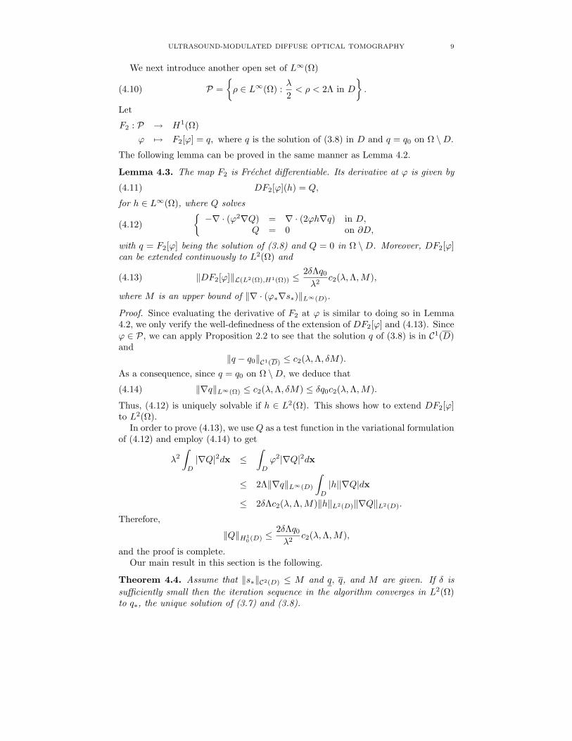
is very small (of order 10−10 in the example in Figure 1).In Figure 2 we consider the same example as in Figure 1. We plot the behaviors

of Eval and Epos as functions of η. It can be seen that the smaller η is, the betteris the reconstruction. However, there is a saturation effect for very small η due tothe finite element discretization.


Figure 2. Reconstruction errors Eval and Epos as functions of η.

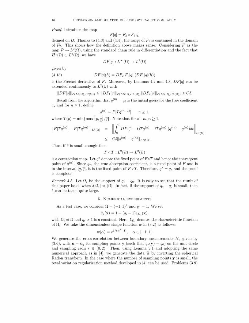
Figure 3. Reconstruction after (from left to right) one, two, andthree iterations with η = 0.02, qi = 3 and Ωi = (−0.25, 0.25)2, andthe measurements Nu are for 50 sources on the unit circle and forr ∈ (0, 2).

Next, we show in Figure 3 that a few iterations are necessary to reconstruct aresolved image if |qi − 1||Ωi|/|Ω| is not too small. In Figure 3, the reconstructedimages after one, two, and three iterations are given. In Figure 4 it can be seen thatwhile the support of the inclusion is quite well reconstructed at the first iteration(it is in fact the support of the data Ψ), a few iterations are needed in order to finda good approximation of the value of the optical absorption parameter.

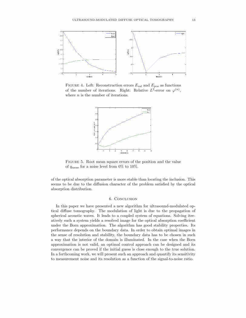
Finally, we illustrate the stability of the proposed algorithm. For doing so, weadd to the measurements a Gaussian white noise with standard deviation rangingfrom 0 to 10% of the L∞ norm ofNu and compute the root mean square errors of theoptical absorption parameter, E(E2

val)1/2, and the position, E(E2

pos)1/2, as functions

of the noise level. Here E stands for the expectation (mean value). In Figure 5,we compute 100 realizations of the measurement noise and apply our algorithm forestimating both the shape and the optical absorption of the inclusion. Figure 5gives, for η = 0.02, E(E2

val)1/2 and E(E2

pos)1/2, as functions of the noise level. It

shows the robustness of the proposed approach. It also shows that finding the value


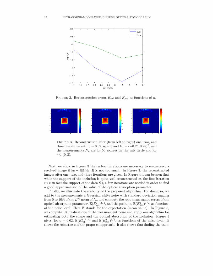
Figure 4. Left: Reconstruction errors Eval and Epos as functions

of the number of iterations. Right: Relative L2-error on ϕ(n),where n is the number of iterations.

Figure 5. Root mean square errors of the position and the valueof qmeas for a noise level from 0% to 10%.

of the optical absorption parameter is more stable than locating the inclusion. Thisseems to be due to the diffusion character of the problem satisfied by the opticalabsorption distribution.

6. Conclusion

In this paper we have presented a new algorithm for ultrasound-modulated op-tical diffuse tomography. The modulation of light is due to the propagation ofspherical acoustic waves. It leads to a coupled system of equations. Solving iter-atively such a system yields a resolved image for the optical absorption coefficientunder the Born approximation. The algorithm has good stability properties. Itsperformance depends on the boundary data. In order to obtain optimal images inthe sense of resolution and stability, the boundary data has to be chosen in sucha way that the interior of the domain is illuminated. In the case when the Bornapproximation is not valid, an optimal control approach can be designed and itsconvergence can be proved if the initial guess is close enough to the true solution.In a forthcoming work, we will present such an approach and quantify its sensitivityto measurement noise and its resolution as a function of the signal-to-noise ratio.


The result of this paper can be extended to acousto-electromagnetic tomographydeveloped in [3]. In [3], the background solution, being a plane wave, has constantamplitude. Even though there is no maximum principle for the Helmholtz equation,the present approach applies to acousto-electromagnetic tomography if one canexplicitly check that the amplitude of the background solution has a positive lowerbound in the domain. This is the case, for example, when the background solutionis a spherical wave emitted at a point outside the domain or in its boundary.

References

[1] H. Ammari, An Introduction to Mathematics of Emerging Biomedical Imaging, Vol. 62, Math-

ematics and Applications, Springer-Verlag, Berlin, 2008.[2] H. Ammari, E. Bonnetier, Y. Capdeboscq, M. Tanter, and M. Fink, Electrical impedance

tomography by elastic deformation, SIAM J. Appl. Math., 68 (2008), pp. 1557–1573.

[3] H. Ammari, E. Bossy, J. Garnier, and L. Seppecher, Acousto-electromagnetic tomography,SIAM J. Appl. Math., submitted.

[4] H. Ammari, E. Bretin, V. Jugnon, and A. Wahab, Photoacoustic imaging for attenuating

acoustic media, Lecture Notes in Math., Vol. 2035, 57–84, Springer-Verlag, Berlin, 2011.

[5] H. Ammari, Y. Capdeboscq, F. de Gournay, A. Rozanova, and F. Triki, Microwave

imaging by elastic perturbation, SIAM J. Appl. Math., 71 (2011), pp. 2112–2130.[6] S. R. Arridge, Optical tomography in medical imaging, Inverse Problems, 15 (1999), R41–

R93.[7] G. Bal and J.C. Schotland, Inverse scattering and acousto-optic imaging, Phys. Rev. Let-

ters, 104 (2010), 043902.

[8] D. A. Boas, D. H. Brooks, E.L. Miller, C. A. DiMarzio, M. Kilmer, R. J. Gaudette, and

Quan Zhang, Imaging the body with diffuse optical tomography, Signal Processing Magazine,

IEEE 18 (2001), 57–75.[9] E. Bossy, A.R. Funke, K. Daoudi, A.C. Boccara, M. Tanter, and M. Fink, Transient

optoelastography in optically diffusive media, Appl. Phys. Lett., 90 (2007), 174111.

[10] Y. Capdeboscq, J. Fehrenbach, F. de Gournay, and O. Kavian, Imaging by modifica-

tion: numerical reconstruction of local conductivities from corresponding power density mea-

surements, SIAM J. Imag. Sci., 2 (2009), pp. 1003–1030.[11] D. S. Elson, R. Li, C. Dunsby, R. Eckersley, and M. X. Tang, Ultrasound-mediated

optical tomography: a review of current methods, Interface Focus, doi:10.1098/rsfs.2011.0021.

[12] M. Giaquinta and E. Giusti, Global C1,α - regularity for second-order quasilinear elliptic

equations in divergence form, Research Report. Centre for Mathematical Analysis, AustralianNational University, 1983.

[13] D. Gilbarg and N. S. Trudinger, Elliptic partial differential equations of second order,Springer-Verlag, Berlin Heidelberg New York, 1977.

[14] P. Gonzalez-Rodrıguez and A. D. Kim, Reflectance optical tomography in epithelial tis-

sues, Inverse Problems, 25 (2009), 015001, 24 pp.[15] D. Hyde, M. Kilmer, D. H. Brooks, and E. Miller, Analysis and exploitation of matrix

structure arising in linearized optical tomographic imaging, SIAM J. Matrix Anal. Appl., 29

(2007), 1065–1082.[16] K. Kilgore, S. Moskow, and J. C. Schotland, Inverse Born series for diffuse waves,

Imaging microstructures, 113–122, Contemp. Math., 494, Amer. Math. Soc., Providence, RI,

2009.[17] O. A. Ladyzhenskaya and N.N. Ural’tseva, Linear and Quasilinear Elliptic Equations,

Translated from the Russian by Scripta Technica, Inc. Translation editor: Leon Ehrenpreis,Academic Press, New York - London, 1968.

[18] G. M. Lieberman, Boundary regularity for solutions of degenerate elliptic equations, Non-

linear Anal., 12 (1988), pp. 1203–1219.[19] G. M. Lieberman, The natural generalization of the natural conditions of Ladyzhenskaya and

Ural’tseva for elliptic equations, Comm. Partial Differential Equations, 16 (1991), pp. 311–361.[20] N. H. Loc and K. Schmitt, On positive solutions of quasilinear elliptic equations, Differen-

tial and Integral Equations, 22 (2009), pp. 829–842.


[21] V. A. Markel and J. C. Schotland, Symmetries, inversion formulas, and image recon-

struction for optical tomography, Phys. Rev. E, 70 (2004), 056616.

[22] S. Moskow and J. C. Schotland, Convergence and stability of the inverse scattering series

for diffuse waves, Inverse Problems, 24 (2008), 065005.

[23] M. H. Protter and H. F. Weinberger, Maximum Principles in Differential Equations,

Prentice-Hall, 1967.[24] M. C. W. van Rossum and Th. M. Nieuwenhuizen, Multiple scattering of classical waves:

microscopy, mesoscopy, and diffusion, Rev. Modern Phys., 71 (1999), 313–371.

[25] L. Ryzhik, G. Papanicolaou, and J. B. Keller, Transport equations for elastic and other

waves in random media, Wave Motion 24 (1996), 327–370.

[26] J. C. Schotland, Direct reconstruction methods in optical tomography, Lecture Notes in

Math., Vol. 2035, pp. 1–29, Springer-Verlag, Berlin, 2011.

[27] J. C. Schotland and V. A. Markel, Inverse scattering with diffusing waves, J. Opt. Soc.

Amer. A, 18 (2001), 2767–2777.

[28] L. V. Wang, Mechanisms of ultrasonic modulation of multiply scattered coherent light: an

analytic model, Phys. Rev. Lett., 87 (2001), 043903.

Department of Mathematics and Applications, Ecole Normale Superieure, 45 Rue

d’Ulm, 75005 Paris, France.

E-mail address: [email protected]

Institut Langevin, ESPCI ParisTech, CNRS UMR 7587, 10 rue Vauquelin, 75231 Paris

Cedex 05, France


Laboratoire de Probabilites et Modeles Aleatoires & Laboratoire Jacques-Louis

Lions, Universite Paris VII, 75205 Paris Cedex 13, France.








Date post:	09-Apr-2020
Category:	Documents
Upload:	others
View:	11 times
Download:	0 times

A RECONSTRUCTION ALGORITHM FOR ULTRASOUND …algorithm for ultrasound-modulated diﬀuse optical...

Documents