A reduced stabilized mixed finite element formulation based on ...

INTERNATIONAL JOURNAL FOR NUMERICAL METHODS IN ENGINEERINGInt. J. Numer. Meth. Engng (2011)Published online in Wiley Online Library (wileyonlinelibrary.com). DOI: 10.1002/nme.3161

A reduced stabilized mixed finite element formulation based onproper orthogonal decomposition for the non-stationary

Navier–Stokes equations

Zhendong Luo1,∗,†, Juan Du2, Zhenghui Xie3 and Yan Guo1

1School of Mathematics and Physics, North China Electric Power University, Beijing 102206,People’s Republic of China

2School of Sciences, Beijing Jiaotong University, Beijing 100044, People’s Republic of China3Institute of Atmospheric Physics, Chinese Academy of Sciences, Beijing 100029, People’s Republic of China

SUMMARY

In this paper, a proper orthogonal decomposition (POD) method is applied to reducing a classical stabilizedmixed finite element (SMFE) formulation for the non-stationary Navier–Stokes equations. Error estimatesbetween the classical SMFE solutions and the reduced SMFE solutions based on the POD method areprovided. The reduced SMFE formulation based on the POD method could not only greatly reduce itsdegrees of freedom but also circumvent the constraint of Brezzi–Babuska (BB) condition so that thecombination of finite element subspaces could be chosen freely and allow optimal-order error estimatesto be obtained. Numerical experiments show that the errors between the reduced SMFE solutions and theclassical SMFE solutions are consistent with theoretical results. Moreover, it is shown that the reducedSMFE formulation based on the POD method is feasible and efficient for solving the non-stationaryNavier–Stokes equations. Copyright � 2011 John Wiley & Sons, Ltd.

Received 18 February 2010; Revised 30 December 2010; Accepted 24 January 2011

KEY WORDS: stabilized mixed finite element method; proper orthogonal decomposition; error estimate;the non-stationary Navier–Stokes equations

1. INTRODUCTION

A mixed finite element (MFE) method is one of the most important approaches for solving the non-stationary Navier–Stokes equations (see [1–5]). However, some fully discrete MFE formulationsfor the non-stationary Navier–Stokes equations include generally many degrees of freedom andan important convergence stability condition is that the Brezzi–Babuska (BB) inequality holds forthe combination of finite element subspaces (see [2–6]). Thus, an important problem is how tocircumvent the constraint of the BB inequality and alleviate the computational load by savingtime-consuming calculations in the computational process in a way that guarantees a sufficientlyaccurate numerical solution.

To circumvent the constraint of BB inequality in MFE methods for stationary Stokes andNavier–Stokes equations, some stabilized finite element methods have been developed (see [7–10]),motivated by streamline diffusion (SD) methods (see [11, 12]). A stabilized SD method for thestationary Navier–Stokes equations is also proposed (see [13]). Some Petrov–Galerkin least-squares

∗Correspondence to: Zhendong Luo, School of Mathematics and Physics, North China Electric Power University,Beijing 102206, People’s Republic of China.

†E-mail: [email protected]

Copyright � 2011 John Wiley & Sons, Ltd.

Z. LUO ET AL.

methods for the stationary Navier–Stokes equations whose residuals are added to are developed(see [14, 15]).

A proper orthogonal decomposition (POD) is a technique offering adequate approximation forrepresenting fluid flow with reduced number of degrees of freedom, i.e. with lower dimensionalmodels to alleviate the computational load and memory requirements (see [16]), which is alsoknown as Karhunen–Loève expansions in signal analysis and pattern recognition (see [17]), orprincipal component analysis in statistics (see [18]), or the method of empirical orthogonal functionsin geophysical fluid dynamics or meteorology (see [19]). The POD method mainly provides auseful tool for efficiently approximating a large amount of data. The method essentially provides anorthogonal basis for representing the given data in a certain least-squares optimal sense, that is, itprovides a way to find optimal lower dimensional approximations of the given data. Combined withsome numerical methods, POD method reduces infinite dimensional PDEs into lower dimensionalmodels so that they could greatly alleviate the computational load and save time for calculationsand resource demands in the computational process.

Although the POD method has been widely applied in computations of statistics, fluid dynamics,design optimization and control (see [16–30]), it is mainly used to perform principal componentanalysis and search the main behavior of a dynamic system, where the method of snapshotswas introduced by Sirovich (see [25]) and was widely applied to reducing the order of PODeigenvalue problem. More recently, some Galerkin POD methods for parabolic problems and ageneral equation in fluid dynamics are presented (see [31, 32]), the singular value decompositionapproach combined with the POD technique is used to treat the Burgers equation (see [33]),and some reduced finite difference schemes and MFE formulations and error estimates for theupper tropical Pacific Ocean model, Burgers equation, the non-stationary Navier–Stokes equations,and parabolic equations based on the POD method were developed (see [34–44]). Moreover,there are some reduced basis methods (or combined with the POD method) for incompressibleviscous/parabolic flows which play an important role in reducing their degrees of freedom andsaving time-consuming calculations and resource demands (see [45–50]).

Although Kragel [51] has derived streamline diffusion POD models in optimization, to the bestof our knowledge, there are no published results addressing the case that combination of the PODmethod with SMFE methods is used to deal with the non-stationary Navier–Stokes equations orproviding error estimates between classical SMFE solutions and reduced SMFE solutions.

In this paper, we extend the developments in [51] and combine SMFE methods with PODmethod to establish a reduced formulation with fewer degrees of freedom for the non-stationaryNavier–Stokes equations. In this manner, we could not only ensure the stabilization of solutions offully discrete SMFE system but also greatly reduce degrees of freedom and save time-consumingcalculations and resource demands in the actual computational process in a way that guaranteesa sufficiently accurate numerical solution. We also derive the error estimates between the clas-sical SMFE solutions and the reduced SMFE solutions based on the POD technique. Numericalexperiments of the physical model of backward facing step flow show that the errors between thereduced SMFE solutions and the classical SMFE solutions are consistent with theoretical results.Moreover, they also show that the reduced SMFE formulation is feasible and efficient for solvingthe non-stationary Navier–Stokes equations.

Although a Petrov–Galerkin least-squares mixed finite element formulation based on the PODmethod for non-stationary conduction–convection problems has also been presented in [52], sincethe non-stationary Navier–Stokes equations and non-stationary conduction–convection problemsdescribe respectively flow of different fluids, the former may be used to describe flow of anyfluid including large-scale flow problem and the cavity flow problem, whereas the latter is mainlyused to describe the flow problem including heat transfer only, which is a very special flow, sothe work in this paper, which is of more widespread applicability than that in [52], is differentfrom that in [52].

The paper is organized as follows. Section 2 is to derive a classical SMFE formulation forthe non-stationary Navier–Stokes equations and to generate snapshots from transient solutionscomputed from the equation system derived by the classical SMFE formulation. In Section 3, theoptimal orthogonal bases are reconstructed from the elements of the snapshots with POD method

Copyright � 2011 John Wiley & Sons, Ltd. Int. J. Numer. Meth. Engng (2011)DOI: 10.1002/nme

STABILIZED MIXED FINITE ELEMENT FORMULATION

and a reduced SMFE formulation with lower dimensional number based on POD method for thenon-stationary Navier–Stokes equations is developed. In Section 4, error estimates between theclassical SMFE solutions and the reduced SMFE solutions based on POD method are derived. InSection 5, some numerical examples are presented illustrating that the errors between the reducedSMFE approximate solutions and the classical SMFE solutions are consistent with previouslyobtained theoretical results, thus validating the feasibility and efficiency of POD method. Section6 provides main conclusions and future tentative ideas.

2. CLASSICAL SMFE APPROXIMATION AND GENERATION OF SNAPSHOTS

Let �⊂R2 be a bounded, connected and polygonal domain. Consider the following non-stationaryNavier–Stokes equations.

Problem (I ): Find u= (u1,u2), p such that for T>0

ut −��u+(u ·∇)u+∇ p= f in �×(0,T )

divu=0 in �×(0,T )

u(x, y, t)=u(x, y, t) on ��×(0,T )

u(x, y,0)=w(x, y) in �

(1)

where u represents the velocity vector, p the pressure, � the constant inverse Reynolds number,f= ( f1, f2) the given body force, u(x, y, t) and w(x, y) are two given vector functions. For the sakeof convenience and without lost generality, we may as well suppose that u(x, y, t) and w(x, y) areall zero vectors in the following theoretical analysis.

The Sobolev spaces along with their properties used in this context are standard (see [53]). Put

X=H10 (�)2, M= L2

0(�)={q∈ L2(�);

∫�qdx dy=0

}

For u, v, w∈ X and q∈M , define

a(u,v)= �∫

�∇u ·∇vdx dy, b(q,v)=

∫�q divvdx dy

a1(u,v,w)= 1

2

∫�

2∑i, j=1

[ui

�v j

�xiw j −ui

�w j

�xiv j

]dx dy

Let N be the positive integer and k=T/N the time step increment. Write tn =kn and un

as an approximation of u(tn)≡u(x, y, tn) (n=1,2, . . . ,N ). By introducing difference quotientapproximation for time derivation of Problem (I), we obtain the following semi-discrete formulationon discrete time.

Problem (II): Find (un, pn)∈ X×M such that, for n=1,2, . . . ,N

(un,v)+ka(un,v)+ka1(un,un,v)−kb(pn,v)=k(fn,v)+(un−1,v) ∀ v∈ X

b(q,un)=0 ∀ q∈M

u0=0 in �

(2)

Using the theory of stationary Navier–Stokes equations may prove that Problem (II) has a uniquesolution (see [4, 5, 54]), and has the following error estimate.

Theorem 2.1If twice derivative utt of the solution (u, p) of Problem (I) is bounded, then

‖u(tn)−un‖0+(k�)1/2n∑

i=1|u(ti )−ui |1+k1/2

n∑i=1

‖p(ti )− pi‖0�Ck


Z. LUO ET AL.

where (u(tn), p(tn)) is the value at tn =kn of the solution (u(t), p(t)) of Problem (I), C is a constantdependent on f and � but independent of k and (u, p).

In order to find the numerical solution for Problem (II), it is necessary to discretize Problem (II)by introducing a MFE approximation for the spatial variable. Let {h} be a uniformly regular familyof triangulation of � (see [54–56]), indexed by a parameter h= max

K∈h{hK ; hK =diam(K )}, i.e.

there is a constant C , independent of h, such that h�ChK (∀K ∈h). We introduce the followingfinite element subspaces Xh ⊂ X and Mh ⊂M

Xh = {vh ∈ X∩C0(�)2;vh |K ∈ P�(K )2∀K ∈h}Mh = {qh ∈M∩C0(�); qh |K ∈ P�(K )∀K ∈h}

(3)

where P�(K ) is the space of piecewise polynomials of degree � on K , ��1 and ��1 are twointegers.

Let (unh, pnh )∈ Xh×Mh be the SMFE approximation corresponding to (un, pn). Then, the fully

discrete SMFE solution for the problem (II) may be written as follows.Problem (III): Find (unh, p

nh )∈ Xh×Mh such that, for 1�n�N

(unh ,vh)+ka(unh,vh)+ka1(unh ,u

nh ,vh)−kb(pnh ,vh)+kb(qh ,u

nh)

+ ∑K∈h

�K (unh −k��unh+k(unh ·∇)unh+k∇ pnh ,vh −k��vh +k(unh ·∇)vh +k∇qh)K

= ∑K∈h

�K (kfn+un−1

h ,vh −k��vh +k(unh ·∇)vh+k∇qh)K

+k(fn,vh)+(un−1h ,vh) ∀(vh ,qh)∈ Xh×Mh u0h =0 in �

(4)

where �K =�hK , �>0 is an arbitrary constant.Write v= (v, p) and w= (w,q). Define

B�(u,unh; v, w) = (v,w)+ka(v,w)+ka1(u,v,w)−kb(p,w)+kb(q,v)

+ ∑K∈h

�K (v−k��v+k(u ·∇)v+k∇ p,w−k��w+k(unh ·∇)w+k∇q)K

F�(w) = ∑K∈h

�K (kfn+un−1

h ,w−k��w+k(unh ·∇)w+k∇q)K +k(fn,w)+(un−1h ,w)

(5)

Then Problem (III) could be rewritten as follows.Problem (IV): Find unh ≡ (unh, p

nh )∈ Xh×Mh such that, for 1�n�N

B�(unh,u

nh; unh, wh)= F�(wh) ∀ wh ≡ (vh,qh)∈ Xh×Mh

u0h =0 in �(6)

Throughout this paper, C indicates a positive constant, and it is possibly different at differentoccurrences, which is independent of the mesh parameters h and time step increment k, but maydepend on �, the Reynolds number, and other parameters introduced in this paper.

The following properties for trilinear form a1(·, ·, ·) are often used (see [1–5, 55]):

a1(u,v,w)=−a1(u,w,v), a(u,v,v)=0 ∀ u,v,w∈ X (7)

The bilinear forms a(·, ·) and b(·, ·) have the following properties:

a(v,v)� �|v|21 ∀ v∈ X (8)

|a(u,v)| � �|u|1|v|1 ∀ u,v∈ X (9)

and

supv∈X

b(q,v)|v|1 ��‖q‖0 ∀ q∈ L2

0(�) (10)



where �>0 is a constant. Define

N0 = supu,v,w∈X

a1(u,v,w)|u|1 ·|v|1 ·|w|1 , ‖f‖−1= sup

v∈X(f,v)|v|1 (11)

The following discrete Gronwall lemma is well known and is very useful in the next analysis(see [2, 4, 5, 54]).

Lemma 2.2 (Gronwall Lemma)If {an}, {bn} and {cn} are three positive sequences, and {cn} is monotone and satisfies

an+bn�cn+ �n−1∑i=0

ai , �>0, a0+b0�c0

then

an+bn�cn exp(n�), n�0

Although �K =�hK here is different from [15], by using the same as the approach in [15], wecan prove the following result.

Theorem 2.3Under the assumptions of Theorem 2.1, Problem (IV) has at least a solution, and if h and k aresufficiently small and h=O(k), then Problem (IV) has a unique solution (unh , p

nh)∈ Xh×Mh such

that [‖unh‖21+

n∑i=1

‖�1/2(uih−k��uih+kuih ·∇uih+k∇ pih)‖20,h]1/2

� (RM)1/2, 0�n�N (12)

‖un−unh‖0+(k�)12

n∑i=1

|ui −uih |1+kn∑

i=1‖pi − pih‖0 � C(h�+h�) (13)

where (un, pn)∈ [H �+1(�)]2×H�+1(�) are the solution to Problem (II), R=�−1, M=(R∑N

i=1 ‖fi‖2−1 +2�h2∑N

i=1 ‖fi‖20)exp(2�h2N ), ‖·‖20,h =∑K∈h‖·‖20,K , C is the constant

dependent on |un |m+1 and |pn |m .Combining Theorems 2.1 and 2.3 yields the following result.

Theorem 2.4Under the assumptions of Theorems 2.1 and 2.3, there are the following error estimates:

‖u(tn)−unh‖0+(k�)1/2n∑

i=1|u(ti )−uih |1+k

12

n∑i=1

‖p(ti )− pih‖0�C(k+h�+h�), 1�n�N

If R=�−1, vector function f, triangulation parameter h, finite elements Xh and Mh and the timestep increment k are given, we can obtain solution ensemble {un1h, un2h , pnh }Nn=1 by solving Problem(III). And then we choose L (in general, L�N , for example, L=20, N =200) instantaneoussolutions (uni1h ,u

ni2h , p

nih )(1�n1<n2< · · ·<nL�N ) (which are useful and of interest to us) from the

N sets of solutions (un1h ,un2h, pnh ) (1�n�N ) to Problem (III), which are known as snapshots.

3. REDUCED SMFE FORMULATION BASED ON POD METHOD

In this section, we use the POD technique to deal with the snapshots in Section 2 and develop areduced SMFE formulation for the non-stationary Navier–Stokes equations.

Let X= X×M and Ui (x, y)= (uni1h ,uni2h , p

nih ) (i =1,2, . . . , L , see Section 2). Set

V= span{U1,U2, . . . ,UL} (14)


Z. LUO ET AL.

and refer to V as ensemble consisting of the snapshots {Ui }Li=1, at least one of which is supposedto be non-zero. Let {w j }lj=1 denote an orthogonal basis of V with l=dimV (l�L). Then eachmember of the ensemble is expressed as

Ui =l∑

j=1(Ui ,w j )Xw j for i =1,2, . . . , L (15)

where (Ui ,w j )X = (uih,wuj)X +(pih,�pj)0, (·, ·)0 is L2-inner product, wuj and �pj are the orthogonalbasis corresponding to u and p, respectively.

The method of POD consists in finding the orthogonal basis such that, for every d (1�d�l),the mean square error between the elements Ui (1�i�L) and corresponding dth partial sum of(15) is minimized on average

min{w j }dj=1

1

L

L∑i=1

∥∥∥∥∥Ui −d∑j=1

(Ui ,w j )Xw j

∥∥∥∥∥2

X

(16)

subject to

(wi ,w j )X =�ij for 1�i�d, 1� j�i (17)

where ‖Ui‖X = [‖∇ui1h‖20+‖∇ui2h‖20+‖pih‖20]1/2. A solution sequence {w j }dj=1 of (16) and (17)is known as a POD basis of rank d.

We introduce the correlation matrix G= (Gij)L×L ∈ RL×L corresponding to the snapshots{Ui }Li=1 by

Gij= 1

L(Ui ,U j )X (18)

The matrix G is positive semi-definite and has rank l. The solution of (16) and (17) can be foundin [20, 25, 42], for example.

Proposition 3.1Let �1��2� · · ·��l>0 denote the positive eigenvalues of G and v1,v2, . . . ,vl the associated eigen-vectors. Then a POD basis of rank d�l is given by

wi =1√�i

L∑j=1

(vi ) jU j , i =1,2, . . . ,d�l (19)

where (vi ) j denotes the j th component of the eigenvector vi . Furthermore, the following errorformula holds:

1

L

L∑i=1

∥∥∥∥∥Ui −d∑j=1

(Ui ,w j )Xw j

∥∥∥∥∥2

X

=l∑

j=d+1� j (20)

Let Vd = span{w1,w2, . . . ,wd} and Xd ×Md =Vd with Xd ⊂ Xh ⊂ X and Md ⊂Mh ⊂M . Setthe Ritz-projection Ph : X→ Xh (if Ph is restricted to the Ritz-projection from Xh to Xd , it iswritten as Pd) such that Ph |Xh = Pd : Xh → Xd and Ph : X\Xh → Xh\Xd and L2-projection d :M→Md denoted by, respectively

a(Phu,vh)=a(u,vh) ∀ vh ∈ Xh (21)

and

(d p,qd)0= (p,qd)0 ∀ qd ∈Md (22)

where u∈ X and p∈M . Owing to (21) and (22) the linear operators Ph and d are well definedand bounded:

‖∇(Pdu)‖0�‖∇u‖0,‖d p‖0�‖p‖0 ∀ u∈ X and p∈M (23)



Lemma 3.2For every d (1�d�l) the projection operators Pd and d satisfy, respectively

1

L

L∑i=1

‖∇(unih −Pdunih )‖20 �l∑

j=d+1� j (24)

1

L

L∑i=1

‖unih −Pdunih ‖20 � Ch2l∑

j=d+1� j (25)

and

1

L

L∑i=1

‖pnih −d pnih ‖20�l∑

j=d+1� j (26)

where unih = (uni1h ,uni2h) and (uni1h ,u

ni2h, p

nih )∈V.

ProofFor any u∈ X we deduce from (21) that

�‖∇(u−Phu)‖20=a(u−Phu,u−Phu)=a(u−Phu,u−vh)

��‖∇(u−Phu)‖0‖∇(u−vh)‖0 ∀vh ∈ Xh

Therefore, we obtain that

‖∇(u−Phu)‖0�‖∇(u−vh)‖0 ∀ vh ∈ Xh (27)

If u=unih , and Ph is restricted to elliptic projection from Xh to Xd , i.e. Phunih = Pdunih ∈ Xd ,

taking vh =∑dj=1(u

nih ,wuj)Xwuj∈ Xd ⊂ Xh (where wuj is the component of w j corresponding to

u) in (27), we can obtain (24) from (20).In order to prove (25), we consider the following variational problem:

(∇w,∇v)= (u−Phu,v) ∀ v∈ X (28)

Thus, w∈ [H10 (�)∩H2(�)]2 and satisfies ‖w‖2�C‖u−Phu‖0. Taking v=u−Phu in (28), from

(27) we obtain that

‖u−Phu‖20 = (∇w,∇(u−Phu))= (∇(w−Phw),∇(u−Phu))

� ‖∇(w−Phw)‖0‖∇(u−Phu)‖0�‖∇(w−wh)‖0‖∇(u−Pdu)‖0 ∀ wh ∈ Xh (29)

Taking wh =hw as linear interpolation of w on �, from the theory of interpolation and (29) wehave

‖u−Phu‖20�Ch‖w‖2‖∇(u−Phu)‖0�Ch‖u−Phu‖0‖∇(u−Phu)‖0Thus, we obtain that

‖u−Phu‖0�Ch‖∇(u−Phu)‖0 (30)

Therefore, if u=unih and Ph is restricted to the Ritz-projection from Xh to Xd , i.e. Phunih =Pdunih ∈ Xd , by (30) and (24) we obtain (25).Using Hölder inequality and (22) yields

‖pnih −d pnih ‖20 = (pnih −d pnih , pnih −d pnih )= (pnih −d pnih , pnih −qd)

� ‖pnih −d pnih ‖0‖pnih −qd‖0 ∀ qd ∈Md

consequently

‖pnih −d pnih ‖0�‖pnih −qd‖0 ∀ qd ∈Md (31)


Z. LUO ET AL.

Taking qd =∑dj=1(p

nih ,�pj)0�pj (where �pj is the component of w j corresponding to p) in (31),

from (20) we can obtain (26), which completes the proof of Lemma 3.2. �

Thus, using Vd = Xd ×Md , we can obtain the reduced SMFE formulation for Problem (III) asfollows.

Problem (V): Find und ≡ (und , pnd )∈Vd such that

B�(und ,u

nd ; und , wn

d)= F�(wnd ) ∀ wn

d ≡ (vd ,qd)∈ Xd×Md , 1�n�N

u0d = 0 (32)

Remark 1Problem (V) is a reduced SMFE formulation based on POD technique for Problem (IV), sinceit only includes 3d freedom degrees while Problem (IV) includes 3Np (where Np is the numberof the nodes in h) if �=�=1, Problem (IV) includes 3Np +3Ns ≈12Np (where Ns is thenumber of the side in h) if �=�=2 and 3d�3Np �12Np (for numerical example in Section 5,d=6, but Np =72×106). And since the residual is introduced, the combination of finite elementsubsets need not satisfy BB stability condition and optimizing order error estimates are yielded.When one computes actual problems, one may obtain the ensemble of snapshots from physicalsystem trajectories by drawing samples from experiments and interpolation (or data assimilation).For example, when one finds numerical solutions to PDEs representing weather forecast, one canuse the previous weather prediction results to construct the ensemble of snapshots, then restructurethe POD optimal basis for the ensemble of snapshots by above (16)–(19), and finally combineit with a SMFE formulation of PDEs representing weather forecast to derive a reduced-ordermodel with fewer degrees of freedom. Thus, the forecast of future weather change can be quicklysimulated, which is a result of major importance for real-life applications.

4. EXISTENCE AND ERROR ANALYSIS OF SOLUTION TO PROBLEM (V)

This section is devoted to discussing the existence and error estimates of solutions to Problem (V).We see from (19) that Vd = Xd×Md ⊂V⊂ Xh×Mh ⊂ X×M . Using the same approaches as

proving Theorem 2.3, we could prove the following existence result for solutions of Problem (V).

Theorem 4.1Under the assumptions of Theorems 2.1 and 2.3, Problem (V) has a unique solution sequence(und , p

nd)∈ Xd ×Md and satisfies, for 1�n�N

[‖und‖21+‖�1/2(und −k��und +kund ·∇und +k∇ pnd )‖20,h]1/2�√RM (33)

In the following theorem, the errors between the solutions (und , pnd ) to Problem (V) and the

solutions (unh , pnh) to Problem (IV) are derived.

Theorem 4.2Under the assumptions of Theorems 2.1 and 2.3, if h and k are sufficiently small, h=O(k),and k=O(L−2), then the errors between the solutions (und , p

nd) to Problem (V) and the solutions

(unh , pnh) to Problem (IV) have the following error estimates, for 1�n�N :

‖unh−und‖0+(k�)12

ni∑j=n1

‖∇(u jh−u j

d)‖0+k1/2ni∑

j=n1

‖p jh − p j

d‖0

�C

(k1/2

l∑j=d+1

� j

)1/2

if n=ni ∈{n1,n2, . . . ,nL} (34)



‖unh−und‖0+(k�)12

[‖∇(unh−und )‖0+

ni∑j=n1

‖∇(u jh−u j

d)‖0]

+k1/2[‖pnh − pnd‖0+

ni∑j=n1

‖p jh − p j

d‖0]

�Ck+C

(k1/2

l∑j=d+1

� j

)1/2

if n �=ni ∈{n1,n2, . . . ,nL} (35)

ProofLet wd = (wn

d ,rnd ), w

nd = Pdunh −und and rnd =d pnh − pnd . On the one hand, we have that

B�(und ,u

nd , wd , wd )=‖wn

d‖20+k�|wnd |21+‖�1/2(wn

d −k��wnd +kund∇wn

d +k∇rnd )‖20,h (36)

On the other hand, if we write Pd u= (Pdunh,d pnh ) and ud = (und , p

dh ), we have that

B�(und ,u

nd , wd , wd)= B�(u

nd ,u

nd , P

d u, wd)−B�(und ,u

nd , ud , wd )

= B�(und ,u

nd , P

d u, wd)−B�(unh,u

nd , u

nh, wd)+(un−1

h −un−1d ,wn

d)

+ ∑K∈h

�K (un−1h −un−1

d , wnd −k��wn

d +kund∇wnd +k∇rnd )K

≡ S1+ S2+ S3+ S4 (37)

where, since a(Pdunh −unh ,wnd)=0

S1 = (Pdunh −unh ,wnd )−kb(d pnh − pnh ,w

nd)

S2 = k[a1(und , Pdunh ,w

nd )−a1(unh,u

nh ,w

nd)+b(rnd , Pdunh−unh)]

S3 = ∑K∈h

�K (Pdunh −unh−k��(Pdunh −unh)+kund∇Pdunh−kunh∇unh

+k∇(d pnh − pnh ), wnd −k��wn


S4 = (un−1h −un−1

d ,wnd)+

∑K∈h

�K (un−1h −un−1

d , wnd −k��wn


Using inverse inequality, Hölder inequality, (7) and Cauchy inequality, and noting that h=O(k),we obtain that

|S1| = |(Pdunh−unh ,wnd)−kb(d pnh − pnh ,w

nd)|

�Ck(|Pdunh−unh |21+‖d pnh − pnh‖20)+ εk�|wnd |21 (38)

|S2| = k|a1(und , Pdunh,wnd )−a1(unh ,u

nh ,w

nd )+b(rnd , Pdunh−unh)|

= k|a1(und , Pdunh−unh,wnd)−a1(w

nd ,u

nh,w

nd)+a1(P

dunh−unh ,und ,w

nd )

− ∑K∈h

(wnd −k��wn

d +kund ·wnd +∇rnd , Pdunh −unh)K

+ ∑K∈h

(wnd −k��wn

d +kund ·wnd , P

dunh−unh)K |

� ε(k�|wnd |21+‖�

12 (wn

d −k��wnd +kund ·wn

d +k∇rnd )‖20,h)+Ck|Pdunh−unh |21+Ckh|wn

d |21 (39)


Z. LUO ET AL.

|S3| =∑

K∈h

�K (Pdunh−unh−k��(Pdunh−unh)+kund∇(Pdunh−unh)

−kwnd∇unh+k(Pdunh −unh)∇unh +k∇(d pnh − pnh ),

wnd −k��wn


�Ck(|Pdunh−unh |21+‖d pnh − pnh‖20)+Ckh|wnd |21

+ε‖�12 (wn


d +k∇rnd )‖20,h (40)

|S4| �Ck|Pdun−1h −un−1

h |21+ 1

2(‖wn−1

d ‖20+‖wnd‖20)+Ck‖wn−1

d ‖20

+ε‖�12 (wn


d +k∇rnd )‖20,h (41)

where ε is a constant which can be chosen arbitrarily. Combining (36) and (37)–(41) yields that

‖wnd‖20+k�|wn

d |21+‖�1/2(wnd −k��wn

d +kund∇wnd +k∇rnd )‖20,h

�Ck(|Pdunh−unh |21+‖d pnh − pnh‖20+|Pdun−1h −un−1

h |21)

+3εk(�|wnd |21+‖�

12 (wn


d +k∇rnd )‖20,h)

+Ckh|wnd |21+ 1

2(‖wn−1

d ‖20+‖wnd‖20)+Ck‖wn−1

d ‖20 (42)

Taking ε�1/4, from (42) we obtain that

‖wnd‖20+k�|wn

d |21+‖�1/2(wnd −k��wn


�Ck(|Pdunh −unh |21+‖d pnh − pnh‖20+|Pdun−1h −un−1

h |21)+Ckh|wn

d |21+‖wn−1d ‖20+Ck‖wn−1

d ‖20 (43)

If h is sufficiently small such that Ch��/2, we yield from the above inequality that

2‖wnd‖20+k�|wn

d |21+2‖�1/2(wnd −k��wn


�Ck(|Pdunh−unh |21+‖d pnh − pnh‖20+|Pdun−1h −un−1

h |21)+2‖wn−1d ‖20+Ck‖wn−1

d ‖20 (44)

First, we consider the case of n∈{n1,n2, . . . ,nL}. Summing (44) from n1 to ni ∈ {n1, n2, . . . ,nL}and let n0=0 using Lemma 3.2 yield that

2‖wnid ‖20+k�

ni∑j=n1

|w jd |21+2

ni∑j=n1

‖�1/2(w jd −k��w j

d +ku jd∇w j

d +k∇r jd )‖20,h

�CkLl∑

j=d+1� j +Ck

ni−1∑i=n0

‖wid‖20 (45)

By using discrete Gronwall inequality, we obtain that

2‖wnid ‖20+k�

ni∑j=n1

|w jd |21+2

ni∑j=n1

‖�1/2(w jd −k��w j

d +ku jd∇w j

d +k∇r jd )‖20,h

�CkLl∑

j=d+1� j exp(Ckn) (46)



If h and k are sufficiently small, k=O(L−2), by using inverse inequality and noting thatnik�kN�T , we obtain that

‖wnid ‖0+(k�)

12

ni∑j=n1

|w jd |1+k

12

ni∑j=n1

‖r id‖0�C

(k1/2

l∑j=d+1

� j

)1/2

(47)

And using Lemma 3.2 yields (34).Next, we consider the case of n �∈ {n1,n2, . . . ,nL}. If n �∈ {n1,n2, . . . ,nL}, we may as well suppose

that tn ∈ (tni , tni+1 ). Expanding unh and pnh into the Taylor series with respect to tni yields that

unh =unih −�k�uh(�1)

�t, �1∈ [ti , tn]; pnh = pnih −�k

�ph(�2)�t

, �2∈ [ti , tn] (48)

where � is the step number from tni to tn . If snapshots are equably taken, then ��N/L . Summing(44) from n1 to ni , n, and using (48), if |�uh(�1)/�t| and |�ph(�2)/�t | are bounded, by discreteGronwall inequality and Lemma 3.2, we obtain that

‖wnd‖20+k�

[|wn

d |21+ni∑

j=n1

|w jd |21]

+k

[‖rnd ‖20+

ni∑j=n1

‖r jd ‖20

]�CkL

l∑j=a+1

� j +Ck3N2/L2 (49)

If k=O(L−2), by (49) we obtain that

‖wnd‖0+(k�)1/2

[|wn

d |21+ni∑

j=n1

|w jd |1]

+k1/2[‖rnd ‖0+

ni∑j=n1

‖r jd ‖20

]

�C

(k1/2

l∑j=a+1

� j

)1/2

+Ck (50)

By (50) and Lemma 3.2, we obtain (35), which completes Theorem 4.2. �

Combining Theorems 2.4 and 4.2 yields the following result.

Theorem 4.3Under hypotheses of Theorems 2.4 and 4.2, the error estimates between the solutions (u(t), p(t))to Problem (I) and the solutions (und , p

nd ) to the reduced SMFE formulation, i.e. Problem (V) are

as follows:

‖u(tn)−und‖0+(k�)12

n∑i=1

‖∇(ui −uid)‖0+k12

n∑i=1

‖pi − pid‖0

�C(h�+h�+k)+C

(k1/2

l∑j=a+1

� j

)1/2

, n=1,2, . . . ,N

Remark 4.4The condition k=O(L−2) in Theorem 4.2 and 35, which implies N =O(L2), shows the relationbetween the number L of snapshots and the number N at all time instances. Moreover, it showsthat it is only necessary to take one snapshot from each 10 transient solutions, optimal-order errorestimates are obtained, but it is unnecessary to take total transient solutions at all time instancestn as snapshots for instance in [31, 32]. Theorems 4.2 and 4.3 have presented the error estimatesbetween the solutions of the reduced SMFE formulation Problem (V) and the solutions of theclassical SMFE formulation Problem (III) and Problem (II), respectively. Our methods employ someclassical SMFE solutions (unih , pnih )(i =1,2, . . . , L) to Problem (III) as assistant analysis. However,when one computes actual problems, one may obtain the ensemble of snapshots from physicalsystem trajectories by drawing samples from experiments and interpolation (or data assimilation).


Z. LUO ET AL.

Thus, the assistant (unih , pnih ) (i =1,2, . . . , L) could be substituted with the interpolation functionsof the experimental and previous results, it is unnecessary to solve Problem (III), and it is onlynecessary to solve directly Problem (V) which includes d freedom degrees (d� l�L�N ).

5. SOME NUMERICAL EXPERIMENTS

In this section, we present some numerical examples of the physical model of backward facingstep flow for first-order element (i.e. �=�=1) and Reynolds number Re=103 by the reducedSMFE formulation Problem (V) validating the feasibility and efficiency of the POD method.

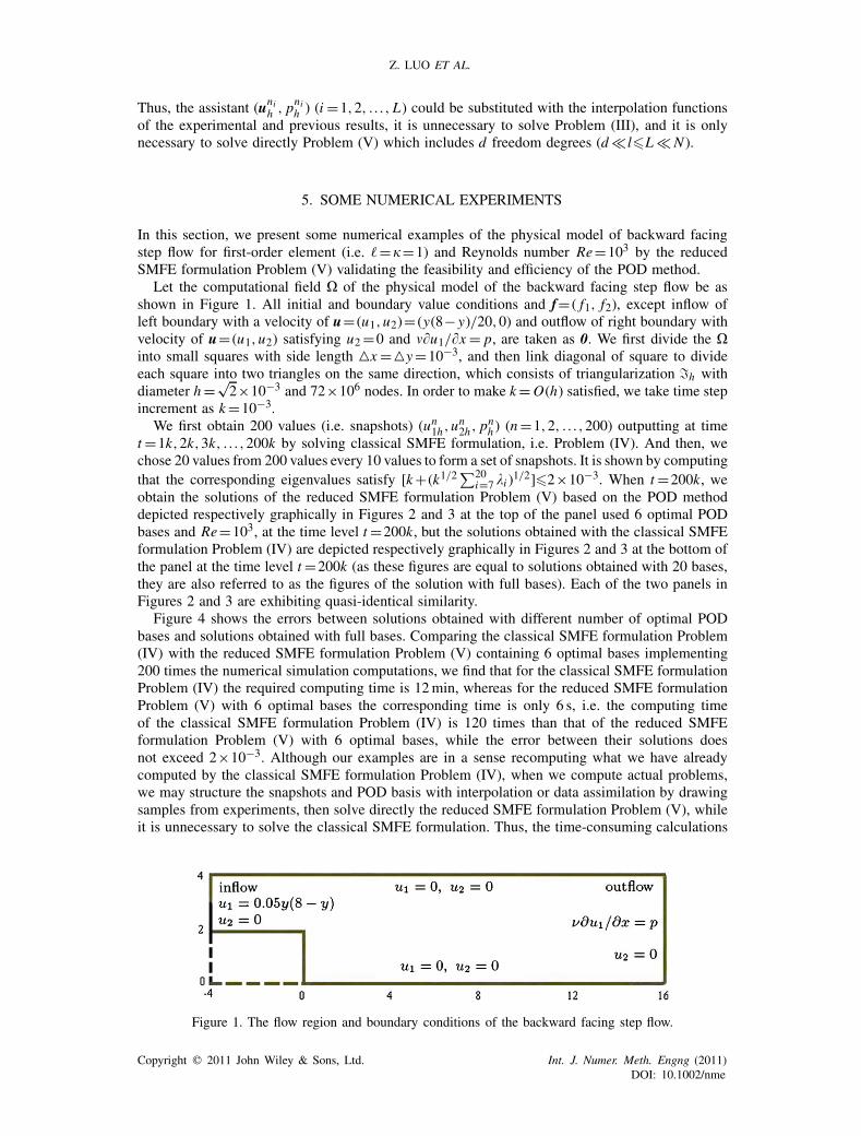
Let the computational field � of the physical model of the backward facing step flow be asshown in Figure 1. All initial and boundary value conditions and f= ( f1, f2), except inflow ofleft boundary with a velocity of u= (u1,u2)= (y(8− y)/20,0) and outflow of right boundary withvelocity of u= (u1,u2) satisfying u2=0 and ��u1/�x = p, are taken as 0. We first divide the �into small squares with side length �x =�y=10−3, and then link diagonal of square to divideeach square into two triangles on the same direction, which consists of triangularization h withdiameter h=√

2×10−3 and 72×106 nodes. In order to make k=O(h) satisfied, we take time stepincrement as k=10−3.

We first obtain 200 values (i.e. snapshots) (un1h ,un2h , p

nh ) (n=1,2, . . . ,200) outputting at time

t=1k,2k,3k, . . . ,200k by solving classical SMFE formulation, i.e. Problem (IV). And then, wechose 20 values from 200 values every 10 values to form a set of snapshots. It is shown by computingthat the corresponding eigenvalues satisfy [k+(k1/2

∑20i=7 �i )1/2]�2×10−3. When t=200k, we

obtain the solutions of the reduced SMFE formulation Problem (V) based on the POD methoddepicted respectively graphically in Figures 2 and 3 at the top of the panel used 6 optimal PODbases and Re=103, at the time level t=200k, but the solutions obtained with the classical SMFEformulation Problem (IV) are depicted respectively graphically in Figures 2 and 3 at the bottom ofthe panel at the time level t=200k (as these figures are equal to solutions obtained with 20 bases,they are also referred to as the figures of the solution with full bases). Each of the two panels inFigures 2 and 3 are exhibiting quasi-identical similarity.

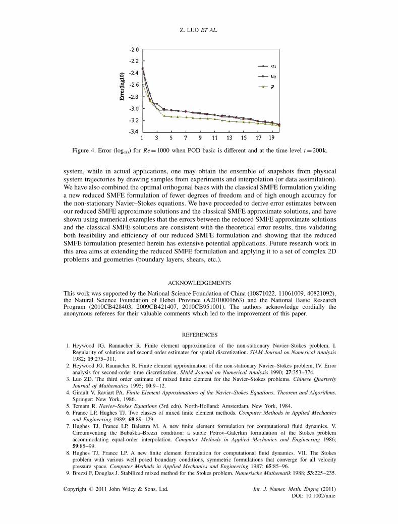
Figure 4 shows the errors between solutions obtained with different number of optimal PODbases and solutions obtained with full bases. Comparing the classical SMFE formulation Problem(IV) with the reduced SMFE formulation Problem (V) containing 6 optimal bases implementing200 times the numerical simulation computations, we find that for the classical SMFE formulationProblem (IV) the required computing time is 12min, whereas for the reduced SMFE formulationProblem (V) with 6 optimal bases the corresponding time is only 6 s, i.e. the computing timeof the classical SMFE formulation Problem (IV) is 120 times than that of the reduced SMFEformulation Problem (V) with 6 optimal bases, while the error between their solutions doesnot exceed 2×10−3. Although our examples are in a sense recomputing what we have alreadycomputed by the classical SMFE formulation Problem (IV), when we compute actual problems,we may structure the snapshots and POD basis with interpolation or data assimilation by drawingsamples from experiments, then solve directly the reduced SMFE formulation Problem (V), whileit is unnecessary to solve the classical SMFE formulation. Thus, the time-consuming calculations

Figure 1. The flow region and boundary conditions of the backward facing step flow.



Figure 2. When Re=1000, comparison of the velocity u field between the classicalSMFE formulation (top panel: at the time level t=200k) and reduced SMFE formulation

(bottom panel: at the time level t=200k).

Figure 3. When Re=1000, comparison of the pressure p field between the classicalSMFE formulation (top panel: at the time level t=200k) and reduced SMFE formulation

(bottom panel: at the time level t=200k).

and resource demands in the computational process will be greatly saved. It is also shown thatfinding the approximate solutions for the non-stationary Navier–Stokes equations with the reducedSMFE formulation Problem (V) is computationally very effective. And the results for numericalexamples are consistent with those obtained for the theoretical case.

6. CONCLUSIONS

In this paper, we have employed the POD techniques to derive a reduced SMFE formulation for thenon-stationary Navier–Stokes equations.We first reconstruct optimal orthogonal bases of ensemblesof data which are compiled from transient solutions derived by using the classical SMFE equation


Z. LUO ET AL.

Figure 4. Error (log10) for Re=1000 when POD basic is different and at the time level t=200k.

system, while in actual applications, one may obtain the ensemble of snapshots from physicalsystem trajectories by drawing samples from experiments and interpolation (or data assimilation).We have also combined the optimal orthogonal bases with the classical SMFE formulation yieldinga new reduced SMFE formulation of fewer degrees of freedom and of high enough accuracy forthe non-stationary Navier–Stokes equations. We have proceeded to derive error estimates betweenour reduced SMFE approximate solutions and the classical SMFE approximate solutions, and haveshown using numerical examples that the errors between the reduced SMFE approximate solutionsand the classical SMFE solutions are consistent with the theoretical error results, thus validatingboth feasibility and efficiency of our reduced SMFE formulation and showing that the reducedSMFE formulation presented herein has extensive potential applications. Future research work inthis area aims at extending the reduced SMFE formulation and applying it to a set of complex 2Dproblems and geometries (boundary layers, shears, etc.).

ACKNOWLEDGEMENTS

This work was supported by the National Science Foundation of China (10871022, 11061009, 40821092),the Natural Science Foundation of Hebei Province (A2010001663) and the National Basic ResearchProgram (2010CB428403, 2009CB421407, 2010CB951001). The authors acknowledge cordially theanonymous referees for their valuable comments which led to the improvement of this paper.

REFERENCES

1. Heywood JG, Rannacher R. Finite element approximation of the non-stationary Navier–Stokes problem, I.Regularity of solutions and second order estimates for spatial discretization. SIAM Journal on Numerical Analysis1982; 19:275–311.

2. Heywood JG, Rannacher R. Finite element approximation of the non-stationary Navier–Stokes problem, IV. Erroranalysis for second-order time discretization. SIAM Journal on Numerical Analysis 1990; 27:353–374.

3. Luo ZD. The third order estimate of mixed finite element for the Navier–Stokes problems. Chinese QuarterlyJournal of Mathematics 1995; 10:9–12.

4. Girault V, Raviart PA. Finite Element Approximations of the Navier–Stokes Equations, Theorem and Algorithms.Springer: New York, 1986.

5. Temam R. Navier–Stokes Equations (3rd edn). North-Holland: Amsterdam, New York, 1984.6. France LP, Hughes TJ. Two classes of mixed finite element methods. Computer Methods in Applied Mechanics

and Engineering 1989; 69:89–129.7. Hughes TJ, France LP, Balestra M. A new finite element formulation for computational fluid dynamics. V.

Circumventing the Bubuska–Brezzi condition: a stable Petrov–Galerkin formulation of the Stokes problemaccommodating equal-order interpolation. Computer Methods in Applied Mechanics and Engineering 1986;59:85–99.

8. Hughes TJ, France LP. A new finite element formulation for computational fluid dynamics. VII. The Stokesproblem with various well posed boundary conditions, symmetric formulations that converge for all velocitypressure space. Computer Methods in Applied Mechanics and Engineering 1987; 65:85–96.

9. Brezzi F, Douglas J. Stabilized mixed method for the Stokes problem. Numerische Mathematik 1988; 53:225–235.



10. Douglas J, Wang JP. An absolutely stabilized finite element method for the stokes problem. Mathematics ofComputation 1989; 52:495–508.

11. Hughes TJ, Tezduyar TE. Finite element methods for first-order hyperbolic systems with particular emphasis onthe compressible Euler equations. Computer Methods in Applied Mechanics and Engineering 1984; 45:217–284.

12. Johnson C, Saranen J. Streamline diffusion methods for the incompressible Euler and Navier–Stokes equations.Mathematics of Computation 1986; 47:1–18.

13. Hansbo P, Szepessy A. A velocity–pressure streamline diffusion finite element method for the incompressibleNavier–Stokes equations. Computer Methods in Applied Mechanics and Engineering 1990; 84:175–192.

14. Zhou TX, Feng MF, Xiong HX. A new approach to stability of finite elements under divergence constraints.Journal of Computational Mathematics 1992; 10:1–15.

15. Zhou TX, Feng MF. A least squares Petrov–Galerkin finite element method for the stationary Navier–Stokesequations. Mathematics of Computation 1993; 60:531–543.

16. Holmes P, Lumley JL, Berkooz G. Turbulence, Coherent Structures, Dynamical Systems and Symmetry. CambridgeUniversity Press: Cambridge, U.K., 1996.

17. Fukunaga K. Introduction to Statistical Recognition. Academic Press: New York, 1990.18. Jolliffe IT. Principal Component Analysis. Springer: Berlin, 2002.19. Selten F. Baroclinic empirical orthogonal functions as basis functions in an atmospheric model. Journal of the

Atmospheric Sciences 1997; 54:2100–2114.20. Berkooz G, Holmes P, Lumley JL. The proper orthogonal decomposition in analysis of turbulent flows. Annual

Review of Fluid Mechanics 1993; 25:539–575.21. Cazemier W, Verstappen RWCP, Veldman AEP. Proper orthogonal decomposition and low-dimensional models

for driven cavity flows. Physics of Fluids 1998; 10:1685–1699.22. Ahlman D, Södelund F, Jackson J, Kurdila A, Shyy W. Proper orthogonal decomposition for time-dependent

lid-driven cavity flows. Numerical Heal Transfer Part B—Fundamentals 2002; 42:285–306.23. Lumley JL. Coherent structures in turbulence. In Transition and Turbulence, Meyer RE (ed.). Academic Press:

New York, 1981; 215–242.24. Aubry N, Holmes P, Lumley JL, Stone E. The dynamics of coherent structures in the wall region of a turbulent

boundary layer. Journal of Fluid Dynamics 1988; 192:115–173.25. Sirovich L. Turbulence and the dynamics of coherent structures: parts I–III. Quarterly of Applied Mathematics

1987; 45:561–590.26. Roslin RD, Gunzburger MD, Nicolaides RA, Erlebacher G, Hussaini MY. A self-contained automated methodology

for optimal flow control validated for transition delay. AIAA Journal 1997; 35:816–824.27. Ly HV, Tran HT. Proper orthogonal decomposition for flow calculations and optimal control in a horizontal CVD

reactor. Quarterly of Applied Mathematics 2002; 60:631–656.28. Ko J, Kurdila AJ, Redionitis OK et al. Synthetic jets, their reduced order modeling and applications to flow

control. AIAA Paper Number 99-1000, 37 Aerospace Sciences Meeting and Exhibit, Reno, 1999.29. Moin P, Moser RD. Characteristic-eddy decomposition of turbulence in channel. Journal of Fluid Mechanics

1989; 200:417–509.30. Rajaee M, Karlsson SKF, Sirovich L. Low dimensional description of free shear flow coherent structures and

their dynamical behavior. Journal of Fluid Mechanics 1994; 258:1401–1402.31. Kunisch K, Volkwein S. Galerkin proper orthogonal decomposition methods for parabolic problems. Numerische

Mathematik 2001; 90:117–148.32. Kunisch K, Volkwein S. Galerkin proper orthogonal decomposition methods for a general equation in fluid

dynamics. SIAM Journal on Numerical Analysis 2002; 40:492–515.33. Kunisch K, Volkwein S. Control of Burgers’ equation by a reduced order approach using proper orthogonal

decomposition. Journal of Optimization Theory and Applications 1999; 102:345–371.34. Cao YH, Zhu J, Luo ZD, Navon IM. Reduced order modeling of the upper tropical Pacific Ocean model using

proper orthogonal decomposition. Computers and Mathematics with Applications 2006; 52:1373–1386.35. Cao YH, Zhu J, Navon IM, Luo ZD. A reduced order approach to four-dimensional variational data assimilation

using proper orthogonal decomposition. International Journal for Numerical Methods in Fluids 2007; 53:1571–1583.

36. Luo ZD, Zhu J, Wang RW, Navon IM. Proper orthogonal decomposition approach and error estimation of mixedfinite element methods for the tropical Pacific Ocean reduced gravity model. Computer Methods in AppliedMechanics and Engineering 2007; 196(41–44):4184–4195.

37. Luo ZD, Chen J, Zhu J, Wang RW, Navon IM. An optimizing reduced order FDS for the tropical Pacific Oceanreduced gravity model. International Journal for Numerical Methods in Fluids 2007; 55(2):143–161.

38. Wang RW, Zhu J, Luo ZD, Navon IM. An Equation-free Reduced Order Modeling Approach to Tropic PacificSimulation. Advances in Geosciences Book Series. World Scientific Publishing: Singapore, 2007.

39. Luo ZD, Wang RW, Zhu J. Finite difference scheme based on proper orthogonal decomposition for the non-stationary Navier–Stokes equations. Science in China Series A: Mathematics 2007; 50(8):1186–1196.

40. Luo ZD, Chen J, Nanvon IM, Yang XZ. Mixed finite element formulation and error estimates based on properorthogonal decomposition for non-stationary Navier–Stokes equations. SIAM Journal on Numerical Analysis 2008;47(1):1–19.


Z. LUO ET AL.

41. Luo ZD, Yang XZ, Zhou YJ. A reduced finite difference scheme based on singular value decomposition andproper orthogonal decomposition for Burgers equation. Journal of Computational and Applied Mathematics 2009;229(1):97–107.

42. Luo ZD, Yang XZ, Zhou YJ. A reduced finite element formulation based on proper orthogonal decompositionfor Burgers equation. Applied Numerical Mathematics 2009; 59(8):1933–1946.

43. Sun P, Luo ZD, Zhou YJ. Some reduced finite difference schemes based on a proper orthogonal decompositiontechnique for parabolic equations. Applied Numerical Mathematics 2010; 60:15–164.

44. Luo ZD, Chen J, Sun P, Yang XZ. Finite element formulation based on proper orthogonal decomposition forparabolic equations. Science in China Series A: Mathematics 2009; 52(3):587–596.

45. Nguyen NC, Rozza G, Patera AT. Reduced basis approximation and a posteriori error estimation for thetime-dependent viscous Burgers’ equation. Calcolo 2009; 46(3):157–185.

46. Nguyen NC, Rozza G, Huynh DBP, Patera AT. Reduced basis approximation and a posteriori error estimationfor parametrized parabolic PDEs; application to real-time Bayesian parameter estimation. In Large-scale InverseProblems and Quantification of Uncertainty, Biegler L, Biros G, Ghattas O, Heinkenschloss M, Keyes D, Mallick B,Marzouk Y, Tenorio L, van Bloemen Waanders B, Willcox K (eds). Wiley: U.K., 2010.

47. Peterson J. The reduced basis method for incompressible flow calculations. SIAM Journal on Scientific Computing1989; 10(4):777–786.

48. Deane AE, Kevrekidis IG, Karniadakis GE, Orszag SA. Low-dimensional models for complex geometry flows:applications to grooved channels and circular cylinders. Physics of Fluids 1991; A3(10):2337–2354.

49. Burkardt J, Gunzburger M, Lee HC. POD and CVT-based reduced-order modeling of Navier–Stokes flows.Computer Methods in Applied Mechanics and Engineering 2006; 196(1–3):337–355.

50. Knezevic DJ, Nguyen NC, Patera AT. Reduced basis approximation and a posteriori error estimation for theparametrized unsteady Boussinesq equations. Mathematical Models and Methods in Applied Sciences. Availablefrom: http://augustine.mit.edu/methodology/papers/atp_M3AS_revised_Jun2010.pdf.

51. Kragel B. Streamline diffusion POD models in optimization. Ph.D. Thesis, Universität Trier, 2005.52. Luo ZD, Chen J, Navon IM, Zhu J. An optimizing reduced PLSMFE formulation for non-stationary conduction–

convection problems. International Journal for Numerical Methods in Fluids 2009; 60(4):409–436.53. Adams RA. Sobolev Space. Academic Press: New York, 1975.54. Luo ZD. Mixed Finite Element Methods and Applications. Chinese Science Press: Beijing, 2006.55. Ciarlet PG. The Finite Element Method for Elliptic Problems. North-Holland: Amsterdam, 1978.56. Brezzi F, Fortin M. Mixed and Hybrid Finite Element Methods. Springer: New York, 1991.


Date post:	29-Jan-2017
Category:	Documents
Upload:	lytuong
View:	218 times
Download:	0 times

A reduced stabilized mixed finite element formulation based on ...

Documents