BIT Numerical Mathematics manuscript No.(will be inserted by the editor)

A Regular Fast Multipole Method for Geometric NumericalIntegrations of Hamiltonian Systems

P. Chartier · E. Darrigrand · E. Faou

Received: date / Accepted: date

Abstract The Fast Multipole Method (FMM) has been widely developed and studied forthe evaluation of Coulomb energy and Coulomb forces. A majorproblem occurs when theFMM is applied to approximate the Coulomb energy and Coulombenergy gradient withingeometric numerical integrations of Hamiltonian systems considered for solving astronomyor molecular-dynamics problems: The FMM approximation involves an approximated po-tential which is not regular. Its lack of regularity impliesa loss of the preservation of theHamiltonian of the system. In this paper, we present a regularization of the Fast MultipoleMethod in order to resume with Hamiltonian preservation. Numerical tests are given on atoy problem to confirm the gain of such a regularization of thefast method.

Keywords Hamiltonian System· Geometric Numerical Integration· Fast MultipoleMethod

1 Introduction

The development of numerical methods that preserve geometric properties of the flow of adifferential equation is motivated by crucial applications in astronomy, molecular dynamics,biology, medecine, ... Intensive studies have been made on symplectic integrators. Nowa-days, the difference between the explicit Euler and the symplectic Euler is an academictopic communly taugth to undergraduate students, and more elaborated schemes such asthe Velocity Verlet scheme are used ([3]). BLABLABLA PARLERDES RESULTATS DUPAPIER D’ERWAN ET PHILIPPE. BLABLABLA [2]. However, the resolution of ordi-nary differential equations still suffer from the time calculation cost, in particular concern-ing molecular dynamics. To resolve the problem of speed, different strategies are consid-ered. One of them consists in using the Fast Multipole Method(FMM) as introduced by L.

P. Chartier· E. Darrigrand· E. FaouEquipe projet IPSO, INRIA Rennes and Ecole Normale Superieure de Cachan - Antenne de Bretagne, AvenueRobert Schumann, 35170 Bruz, FranceE-mail: chartier@irisa.fr , eric.darrigrand-lacarrieu@univ-rennes1.fr , efaou@irisa.fr

E. DarrigrandIRMAR - Universite de Rennes 1, Campus de Beaulieu, 35042 Rennes cedex, France

2

Greengard and V. Rokhlin ([14]). This first version was written to deal with point charges.In papers [13], [12], [11], [7] and [5], the FMM was extended to and developed for the caseof continuous distributions of the charges which corresponds to the charge distributions inmolecular dynamics. The improvements led to versions of FMMrefered as the continuousor gaussian Fast Multipole Method (CFMM or GFMM).

However, the results obtained with the FMM, CFMM, GFMM were not satisfying fortwo reasons: First, the FMM is affecting the symplectic property of geometric integrators. Toattenuate this impact of the FMM, users decide to use a large or huge number of multipolesin the FMM expansions (up toL = 20 whereL denotes the number of multipoles). Secondly,the FMM in its original form has a translation step which costs O(L4) as a function ofL.The translation step is then very costly when the required accuracy motivates the choice ofa large or hugeL. Motivated by these incovenients of the FMM, many improvements weredone to reduce the time requirements of the translation step: Elliot and Board reduced theO(L4) cost toO(L2 lnL) in [17] ; Petersenet al. ([18]) adjusted the number of multipolesto the boxes leading to the “very” Fast Multipole Method (vFMM), also adapted to the caseof continuous distributions (GvFMM) in [5], [6] and [7] ; Rotation matrices enable one toapply translations in specific directions for which the calculation reduces to an expressionwhich is significantly cheaper (see [10], [15]). Further improvements consisted in adaptingthe FMM to periodic structures ([4], [8], [9], ...). Later on, Greengard and Huang suggesteda new FMM based on another expansion ([16]) that we will not discuss in this paper.

In this paper, we do not focus on any way to perform the translation but try to make theFMM preserving the properties of the geometric integrators. Indeed, the FMM deterioratesthe good properties of the potential partly because the approximated potential is not regularsince the FMM approximation is obtained by splitting the volume domain into some boxesand writing an expansion that depends on these boxes. The loss of the regularity widelyaffects the symplectic property of the integrators. We theninvestigate a new FMM whichis regular at the interface between the boxes and then gives aregular approximation of thepotential. We will refer to the new version as the Regular Fast Multipole Method (RFMM).

The following section introduces the Fast Multipole Methodand the drawback of its nonregularity and suggests a regularizing technic: The Regular FMM (RFMM) is explained inSubsection 2.2. An application of the RFMM and a comparison with the classical FMM aregiven in Section 3 where the methods are applied within the Velocity Verlet scheme.

2 Regularization of a Fast Multipole Method

In this section, we first explain the Fast Multipole Method asinvolved in this paper. Theregularizing technic is derived in a second part.

2.1 A classical Fast Multipole Method

We briefly describe the Fast Multipole Method as derived in [14] and explicitly written in[15]. This method has supported several improvements in term of complexity cost regard-ing a special step that is usually called “translation” and sometimes called “transfer”. For asick of simplicity, we will consider a basic Fast Multipole Method and then apply our reg-ularization to a relatively simple algorithm. Of course, the regularization technic could beapplied in the same manner to improved versions of the Fast Multipole Method as developed

3

in [17], [18], [10] and [15] for example. Moreover, we first focus our attention on a one-levelalgorithm.

2.1.1 The FMM expansion for a standard kernel

Somehow, in many situations, the application of the Fast Multipole Method is involved tospeed up matrix-vector productsAq with q a given vector andA the matrix defined by:∀i, j ∈ {1, ...,N}

Ai j =1

∥

∥xi −x j∥

∥

wherex1, ..., xN areN points of a bounded domainD of R3 and‖·‖ denotes the Euclidian

norm onR3. When one calculates(Aq)i = ∑N

j=11

‖xi−x j‖q j for a giveni, one usually calls

xi the target point andx j the source points. The source points are first distributed ingroupswhich correspond to a partition of the domainD. Let us denote byB the set of those groups.We will also denote byB. (for example:Bsrc, Btrg), andC. (for example:Csrc, Ctrg), thegroups ofB and their centers respectively.

To approximate the calculation of(Aq)i , we split the summation as follows,

(Aq)i = ∑Bsrc close toBtrg

∑x j∈Bsrc

1∥

∥xi −x j∥

∥

q j

= ∑Bsrc far from Btrg

∑x j∈Bsrc

1∥

∥xi −x j∥

∥

q j

whereBtrg denotes the group which contains the target pointxi . The first term is not approx-imated and is calculated exactly. The second term is approximated thanks to the multipoleexpansion and a translation operator that makes the conversion of the multipole expansionto the local expansion (for details, see Appendix 5.1 or [14], [15]).

The algorithm for the calculation of the matrix-vector product Aq can be written in thisform:

• Step 0: Calculation of someq-independant quantities.· Precalculation related to the translation operatorsTBtrg Bsrc that converts a multipole

expansion aroundCsrc to a local expansion aroundCtrg.

· The far momentsf l ,kj and the local momentsgl ,k

i involved in the multipole and localexpansions, for each source pointsx j or target pointsxi .

• Step 1: Calculation of the far fields:∀Bsrc∈B, F l ,kBsrc

accumulates the chargesq j together

with the far momentsf l ,kj of the source points contained inBsrc.

• Step 2: Calculation of the local fields:∀Btrg ∈ B, (Gl ,kBtrg

)l ,k is obtained by translations

of the far fields(Fλ ,κBsrc

)λ ,κ for all Bsrc ∈ B far from Btrg.

• Step 3: Accumulation of the far interactions:∀Btrg ∈B, ∀xi ∈ Btrg, (Aq) f ari accumulates

the local fields(Gl ,kBtrg

)l ,k together with the local moments(gl ,ki )l ,k.

• Step 4: Calculation of the close interactions:∀Btrg ∈B,∀xi ∈Btrg, (Aq)closei accumulates

the contribution of the neighbor source pointsx j .• Step 5: Calculation of matrix-vector product:∀Btrg ∈ B, ∀xi ∈ Btrg,

(Aq)i ≈ (Aq)closei +(Aq) f ar

i (1)

4

•CBT

CBS1• •CBS2

xi1◦

x j1◦ ◦x j2

CBT1• •CBT2

xi1◦ ◦xi2

Far interactions ofBT1

Far interactions ofBT2

Close interactions ofxi1 ∈ BT1

Close interactions ofxi2 ∈ BT2

(a) (b)

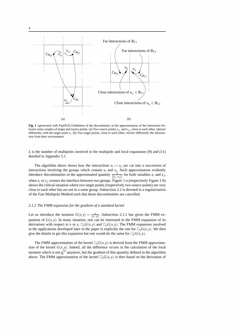
Fig. 1 (generated with Fig4TeX) Exhibition of the discontinuity in the approximation of the interaction be-tween some couples of target and source points. (a) Two source pointsxj1 andxj2 , close to each other, interactdifferently with the target pointxi . (b) Two target points, close to each other, receive differently the informa-tion from their environment.

L is the number of multipoles involved in the multipole and local expansions (9) and (11)detailed in Appendix 5.1.

The algorithm above shows how the interactionsxi ↔ x j are cut into a succession ofinteractions involving the groups which containxi andx j . Such approximation evidentlyintroduce discontinuities in the approximated quantity1

‖xi−x j‖ for both variablesxi andx j ,

whenxi or x j crosses the interface between two groups. Figure 1-a (respectively Figure 1-b)shows the critical situation where two target points (respectively two source points) are veryclose to each other but are not in a same group. Subsection 2.2is devoted to a regularizationof the Fast Multipole Method such that those discontinuities are cancelled.

2.1.2 The FMM expansion for the gradient of a standard kernel

Let us introduce the notationG(x,y) = 1‖x−y‖ . Subsection 2.1.1 has given the FMM ex-

pansion ofG(x,y). In many situation, one can be interested in the FMM expansion of itsderivatives with respect tox or y, ∇xG(x,y) and∇yG(x,y). The FMM expansion involvedin the applications developed later in the paper is explicitly the one for∇xG(x,y). We thengive the details to get this expansion but one would do the same for ∇yG(x,y).

The FMM approximation of the kernel∇xG(x,y) is derived from the FMM approxima-tion of the kernelG(x,y). Indeed, all the difference occurs in the calculation of thelocalmoment which is notgl ,k

i anymore, but the gradient of this quantity defined in the algorithmabove. The FMM approximation of the kernel∇xG(x,y) is then based on the derivation of

5

the quantitygl ,ki with respect toxi . This derivation is easy to perform when we remark that

the quantitygl ,ki is polynomial with respect to(xi −Ctrg). Details are given in Appendix 5.2

about our way to perform this derivation.

2.2 A Regularized Version of the Fast Multipole Method

As explained in Subsection 2.1, we apply a regularization technic to a rather basic one-levelFast Multipole Method but it can easily be extended to improved versions as the ones de-veloped in [17], [18], [10], [15], .... At the end of the subsection, we discuss the multilevelversion. Moreover, the multi-dimensional regularizationis obtained by considering a 1Dregularization in each direction. The 3D regularization isobtained by considering a 1D reg-ularization on each component of the 3D variable. So, in thissubsection, we mainly focusour attention on the 1D regularization of the FMM approximation of the kernelG(x,y). Theregularized FMM approximation of its derivatives is obtained considering the derivatives ofthe regularized FMM approximation of the kernel.

2.2.1 A 1D regularization

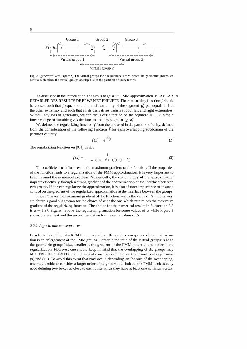
As pointed out in Subsection 2.1, the FMM introduces a discontinuity related to the distribu-tion of the domain points into groups. The discontinuities appear at the interface between thegroups. In this paper, we organize the regularization with the simple following idea: when apoint of a group is close to another group, we consider it as a point of both groups, the onethat effectively contains it and the one which is close to this point. So, the point is consideredas contained in two groups and its contribution to each of thegroups is calculated accordingto its location. This consideration leads to a new distribution of the points. We designate thegroups associated to this distribution as virtual groups.

Below, we illustrate the idea of the regularization appliedto the target variable. In Figure2, the pointsgl

i , gi andgri are defined such that thei-th geometric group is[gi ,gi+1] and the

i-th virtual group is[gli ,g

ri+1]. In Figure 2, the pointx1 is considered as contained in group

2 only, with a coefficient of contribution equal to 1, and relation (1) remains the same.The pointx2 is considered as contained in groups 2 and 3, with coefficients of contributionrespectively equal toc2 andc3 such that:

⋆ c2 +c3 = 1 ; obviously,c2 > c3.⋆ c2 andc3 are given by a regularizing functionf : [gl

3,gr3] → [0,1],

c2 = (1− f (x2)) , c3 = f (x2) such that (1) becomes

(Aq)x2 ≈ (1− f (x2)) [(Aq)closex2∈ group2 +(Aq) f ar

x2∈ group2]

+ f (x2) [(Aq)closex2∈ group3 +(Aq) f ar

x2∈ group3]

The pointx3 is considered as contained in groups 1 and 2, with coefficients of contributionrespectively equal toc1 andc2 such that:

⋆ c1 +c2 = 1 ; obviously,c1 < c2.⋆ c1 andc2 are given by a regularizing functionf : [gl

2,gr2] → [0,1],

c1 = (1− f (x3)), c2 = f (x3) such that (1) becomes

(Aq)x3 ≈ (1− f (x3)) [(Aq)closex3∈ group1 +(Aq) f ar

x3∈ group1]

+ f (x3) [(Aq)closex3∈ group2 +(Aq) f ar

x3∈ group2]

6

Virtual group 1

Virtual group 2

Virtual group 3

Group 1 Group 2 Group 3

g1gl1 gr

1x1•

x2•x3•

Fig. 2 (generated with Fig4TeX) The virtual groups for a regularized FMM: when the geometric groups arenext to each other, the virtual groups overlap like in the partition of unity technic.

As discussed in the introduction, the aim is to get aC∞ FMM approximation. BLABLABLAREPARLER DES RESULTS DE ERWAN ET PHILIPPE. The regularizingfunction f shouldbe chosen such thatf equals to 0 at the left extremity of the segment[gl

i ,gri ], equals to 1 at

the other extremity and such that all its derivatives vanishat both left and right extremities.Without any loss of generality, we can focus our attention onthe segment[0,1]. A simplelinear change of variable gives the function on any segment[gl

i ,gri ].

We defined the regularizing functionf from the one used in the partition of unity, definedfrom the consideration of the following functionf for each overlapping subdomain of thepartition of unity.

f (x) = e−α

1−x2 (2)

The regularizing function on[0,1] writes

f (x) =1

1+e−a[1/(1−x2)−1/(1−(x−1)2)](3)

The coefficientα influences on the maximum gradient of the function. If the propertiesof the function leads to a regularization of the FMM approximation, it is very important tokeep in mind the numerical problem. Numerically, the discontinuity of the approximationimpacts effectively through a strong gradient of the approximation at the interface betweentwo groups. If one can regularize the approximation, it is also of most importance to ensure acontrol on the gradient of the regularized approximation atthe interface between the groups.

Figure 3 gives the maximum gradient of the function versus the value ofα . In this way,we obtain a good suggestion for the choice ofα as the one which minimizes the maximumgradient of the regularizing function. The choice for the numerical results in Subsection 3.3is α = 1.37. Figure 4 shows the regularizing function for some valuesof α while Figure 5shows the gradient and the second derivative for the same values ofα .

2.2.2 Algorithmic consequences

Beside the obtention of a RFMM approximation, the major consequence of the regulariza-tion is an enlargement of the FMM groups. Larger is the ratio of the virtual groups’ size tothe geometric groups’ size, smaller is the gradient of the FMM potential and better is theregularization. However, one should keep in mind that the overlapping of the groups mayMETTRE EN DEFAUT the conditions of convergence of the multipole and local expansions(9) and (11). To avoid this event that may occur, depending onthe size of the overlapping,one may decide to consider a larger order of neighborhood. Indeed, the FMM is classicallyused defining two boxes as close to each other when they have atleast one commun vertex:

7

0.5 1 1.5 2 2.5 31.4

1.6

1.8

2

2.2

2.4

2.6

2.8Max grad of smoothing exp infty fct versus alpha

grad(alpha)

1.3 1.32 1.34 1.36 1.38 1.4 1.421.54

1.5405

1.541

1.5415

1.542

1.5425

1.543Max grad of smoothing exp infty fct versus alpha −− ZOOM

grad(alpha)

(a) (b)

Fig. 3 (a) The maximum gradient of the regularizing function versus α . (b) Zoom around the optimal valueof α .

0 0.1 0.2 0.3 0.4 0.5 0.6 0.7 0.8 0.9 10

0.1

0.2

0.3

0.4

0.5

0.6

0.7

0.8

0.9

1

Smoothing function Exp Infty with different alphas

alpha = 3 log 2alpha = 1.2alpha = 1.36alpha = 1.5

Fig. 4 Plot of the regularizing functions for some values ofα (3 log2, 1.2, 1.36, 1.5).

0 0.1 0.2 0.3 0.4 0.5 0.6 0.7 0.8 0.9 10

0.2

0.4

0.6

0.8

1

1.2

1.4

1.6

1.8

2

Grad smoothing function Exp Infty with different alphas

alpha = 3 log 2alpha = 1.2alpha = 1.36alpha = 1.5

0 0.1 0.2 0.3 0.4 0.5 0.6 0.7 0.8 0.9 1−20

−15

−10

−5

0

5

10

15

20

Grad2 smoothing function Exp Infty with different alphas

alpha = 3 log 2alpha = 1.2alpha = 1.36alpha = 1.5

(a) (b)

Fig. 5 (a) Plot of the first derivative of regularizing functions for α = 3log2, 1.2, 1.36, 1.5. (b) Plot of thesecond derivative of regularizing functions forα = 3log2, 1.2, 1.36, 1.5.

8

We say that they are neighbor of order 1. And, we defineB1 andB2 as neighbor of order 2if there is at least one boxB3 such thatB1 andB3 are neighbor of order 1 andB2 andB3 areneighbor of order 1. The order of neighborhood can be numerically caracterized using theinfinity norm when the groups are cubes from a usual FMM oc-tree.

The overlapping leads to a distribution where each point is contained in more than onegroup. For each group, each point is associated to a contribution coefficient that says howthe point should contribute in the calculation as a point of the current group.

The regularization can be performed for both the first and thesecond variables of thekernel 1

‖xi−x j‖ . But, in a usual situation, one may be interested in the regularization for the

target variable only. When the regularization occurs on thesource point, then the contribu-tion coefficient applies in the calculation of the far fields (19) in the FMM algorithm andonly the source points are distributed in overlapping groups. When the regularization occurson the target point, the contribution coefficient is involved in the last step (1) and only thetarget points are distributed in overlapping groups. In this paper, we are interested in a reg-ularization for the target points only.

Now, we should specify the impact of the regularization on the complexity of the FMM.The increase of the FMM calculation occurs only in the fact that some target points belongto two groups. The over-cost then occurs only in the last stepof the calculation of the farinteractions (Step 3, relation (21)) and in the step of calculation of the close interactions(Step 4, relation (22)) in the FMM algorithm. The cost of Steps 3 and 4 is multiplied by theratio between the average number of points in the virtual groups and the average number ofpoints in the geometric group; but the complexity of these steps remains the same. Finally,the complexity of the entire algorithm does not change. Moreover, the only steps which areaffected by the regularization, in term of increase of the cost, are not significant steps in thesense that the most costly one is the step of translations that computes the local fields fromthe global fields (Step 2, relation (20)).

2.2.3 Error estimates

Is there anything easy to do on error estimates ??? BLABLABLA. If yes, it may involverelations (10),(14).

2.2.4 Application of the regularization to a 1D distribution of points

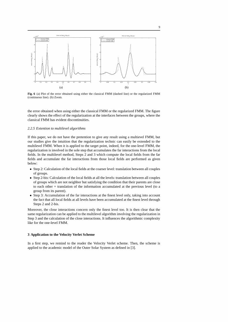
As an illustration of the regularization of the FMM, we consider here a set of 800 pointsx1, ...,x800, uniformly distributed on the 1D domain[0,1]. For this illustration, we computea vectorS defined by: fori = 1, ...,800, Si = ∑400

j=250G(xi ,x j) with G(xi ,x j) = 1‖xi−x j‖ if

i 6= j and 0 otherwise. The quantityS can be defined as a classical matrix-vector productcommunly computed with the FMM. Here, we computedS in three different ways: exactcalculation, using a classical FMM and using a regularized FMM. Figure 6 gives plots of

9

0 0.1 0.2 0.3 0.4 0.5 0.6 0.7 0.8 0.9 1−2

0

2

4

6

8

10x 10

−3

x

erro

r on

Sum

y( G

(x,y

) )

Error on Sumy( G(x,y) )

classical FMMsmooth FMM

0 0.05 0.1 0.15 0.2 0.25 0.3 0.35 0.4−2

0

2

4

6

8

10x 10

−3

x

erro

r on

Sum

y( G

(x,y

) )

Error on Sumy( G(x,y) )

classical FMMsmooth FMM

(a) (b)

Fig. 6 (a) Plot of the error obtained using either the classical FMM(dashed line) or the regularized FMM(continuous line). (b) Zoom.

the error obtained when using either the classical FMM or theregularized FMM. The figureclearly shows the effect of the regularization at the interfaces between the groups, where theclassical FMM has evident discontinuities.

2.2.5 Extention to multilevel algorithms

If this paper, we do not have the pretention to give any resultusing a multievel FMM, butour studies give the intuition that the regularization technic can easily be extended to themultilevel FMM. When it is applied to the target point, indeed, for the one-level FMM, theregularization is involved in the sole step that accumulates the far interactions from the localfields. In the multilevel method, Steps 2 and 3 which compute the local fields from the farfields and accumulate the far interactions from those local fields are performed as givenbelow:

• Step 2: Calculation of the local fields at the coarser level: translation between all couplesof groups.

• Step 2-bis: Calculation of the local fields at all the levels:translation between all couplesof groups which are not neighbor but satisfying the condition that their parents are closeto each other + translation of the information accumulated at the previous level (to agroup from its parent).

• Step 3: Accumulation of the far interactions at the finest level only, taking into accountthe fact that all local fields at all levels have been accumulated at the finest level throughSteps 2 and 2-bis.

Moreover, the close interactions concern only the finest level too. It is then clear that thesame regularization can be applied to the multilevel algorithm involving the regularization inStep 3 and the calculation of the close interactions. It influences the algorithmic complexitylike for the one-level FMM.

3 Application to the Velocity Verlet Scheme

In a first step, we remind to the reader the Velocity Verlet scheme. Then, the scheme isapplied to the academic model of the Outer Solar System as defined in [3].

10

3.1 The Velocity Verlet Scheme or Stormer Verlet Scheme

Hamiltonian systems have motivated several researches on investigation of schemes thatsolve ODEs preserving the geometric invariants of these systems. A famous and widelyused one is the Velocity Verlet method. We present hereby thescheme as a tool adapted tothe solution of Hamiltonian systems of the form

{

q = M−1pp = −∇U(q)

(4)

whereM = diag(m1I , · · · ,mNI) and I is the 3-dimensional identity matrix. The system isequivalent to the special second order differential equation

q = f (q),

where the right-hand sidef (q) = −M−1∇U(q) does not depend on ˙q.The Hamiltonian of the system writes

H(p,q) = T(p)+U(q) (5)

whereT is a quadratic function.The Stormer Verlet Scheme writes (CHECK NAME .....................)

vn+ 12

= vn + h2 f (qn)

qn+1 = qn +hvn+ 12

vn+1 = vn+ 12+ h

2 f (qn+1)

(6)

and the Velocity Verlet Scheme writes (CHECK NAME .....................)

qn+ 12

= qn + h2vn

vn+1 = vn +h f(qn+ 12)

qn+1 = qn+ 12+ h

2vn+1

(7)

whereqn (resp.vn) denotes an approximation ofq(nh) (resp.v(nh)) andv= q= M−1p. Theschemes are explicit one-step methods which is very convenient for actual computation. Ifone does not need the values of the velocityvn, the first and the third equations in (6) can bereplaced by

vn+ 12

= vn− 12+h f(qn).

When the scheme is applied to astronomy or molecular dynamics, the calculation of thequantities f (q) for successive vectorsq corresponds to the most costly part of the entirecomputation. The cost of the standard calculation off (q) for a givenq is of orderN2 whenall the other steps of the scheme have a cost of orderN. The implication of the FMM con-sists in reducing the cost of the calculation off (q) for given q which is more or less thecalculation of∇U(q).

11

3.2 FMM and the Outer Solar System

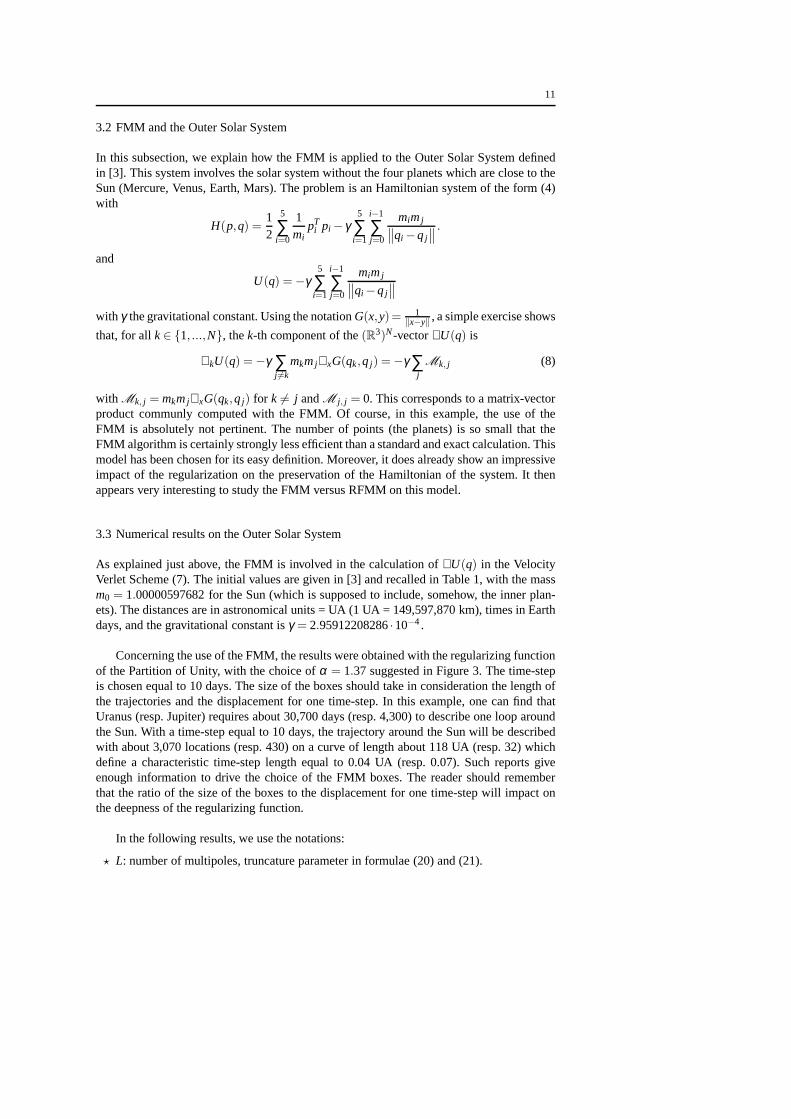
In this subsection, we explain how the FMM is applied to the Outer Solar System definedin [3]. This system involves the solar system without the four planets which are close to theSun (Mercure, Venus, Earth, Mars). The problem is an Hamiltonian system of the form (4)with

H(p,q) =12

5

∑i=0

1mi

pTi pi − γ

5

∑i=1

i−1

∑j=0

mimj∥

∥qi −q j∥

∥

.

and

U(q) = −γ5

∑i=1

i−1

∑j=0

mimj∥

∥qi −q j∥

∥

with γ the gravitational constant. Using the notationG(x,y)= 1‖x−y‖ , a simple exercise shows

that, for allk∈ {1, ...,N}, thek-th component of the(R3)N-vector∇U(q) is

∇kU(q) = −γ ∑j 6=k

mkmj ∇xG(qk,q j) = −γ ∑j

Mk, j (8)

with Mk, j = mkmj∇xG(qk,q j) for k 6= j andM j, j = 0. This corresponds to a matrix-vectorproduct communly computed with the FMM. Of course, in this example, the use of theFMM is absolutely not pertinent. The number of points (the planets) is so small that theFMM algorithm is certainly strongly less efficient than a standard and exact calculation. Thismodel has been chosen for its easy definition. Moreover, it does already show an impressiveimpact of the regularization on the preservation of the Hamiltonian of the system. It thenappears very interesting to study the FMM versus RFMM on thismodel.

3.3 Numerical results on the Outer Solar System

As explained just above, the FMM is involved in the calculation of ∇U(q) in the VelocityVerlet Scheme (7). The initial values are given in [3] and recalled in Table 1, with the massm0 = 1.00000597682 for the Sun (which is supposed to include, somehow, the inner plan-ets). The distances are in astronomical units = UA (1 UA = 149,597,870 km), times in Earthdays, and the gravitational constant isγ = 2.95912208286·10−4.

Concerning the use of the FMM, the results were obtained withthe regularizing functionof the Partition of Unity, with the choice ofα = 1.37 suggested in Figure 3. The time-stepis chosen equal to 10 days. The size of the boxes should take inconsideration the length ofthe trajectories and the displacement for one time-step. Inthis example, one can find thatUranus (resp. Jupiter) requires about 30,700 days (resp. 4,300) to describe one loop aroundthe Sun. With a time-step equal to 10 days, the trajectory around the Sun will be describedwith about 3,070 locations (resp. 430) on a curve of length about 118 UA (resp. 32) whichdefine a characteristic time-step length equal to 0.04 UA (resp. 0.07). Such reports giveenough information to drive the choice of the FMM boxes. The reader should rememberthat the ratio of the size of the boxes to the displacement forone time-step will impact onthe deepness of the regularizing function.

In the following results, we use the notations:

⋆ L: number of multipoles, truncature parameter in formulae (20) and (21).

12

Table 1 Data for the Outer Solar System

planet/Sun mass initial position initial velocity

Sun m0 (0 , 0 , 0) (0 , 0 , 0)

Jupiter m1 = 0.000954786104043-3.5023653-3.8169847-1.5507963

0.00565429-0.00412490-0.00190589

Saturn m2 = 0.0002855837331519.0755314-3.0458353-1.6483708

0.001683180.004835250.00192462

Uranus m3 = 0.00004372731645468.3101420

-16.2901086-7.2521278

0.003541780.001371020.00055029

Neptune m4 = 0.000051775913844911.4707666-25.7294829-10.8169456

0.002889300.001145270.00039677

Pluto m5 = 11.3·108

-15.5387357-25.2225594-3.1902382

0.00276725-0.00170702-0.00136504

⋆ No: order of neighborhood that defines the close and far interactions in the FMM oc-tree.

⋆ NL: number of levels of the oc-tree.⋆ ht : time-step size.⋆ Rreg: ratio of the regularization zone on each side of a geometricgroup to the length

of the geometric group. Example: For the 1D group[0,1], whenRreg = 0.25, the vir-tual corresponding group is[−0.25,1.25] and the regularization function operates on[−0.25,0.25] and[−0.75,1.25].

As well known, the FMM behaves as geometric series with respect toL. Classical appli-cations of the FMM would imply a choice ofL around 6. A very precise but costly choice (asused in molecular dynamics) would beL around 15 and even more, around 20. The choiceL = 3 definitely generates an unprecise FMM approximation. In the following tests, we con-fronted the regularized FMM approximation to the choiceL = 3, 5, 6 and 10. Moreover, wefound that a good compromise for the choice of the number of levels wasNL = 7. In a firsttime, we will considerRreg = 0.25 with an order of neighborhoodNo = 1. We will thenshow results withRreg = 0.45 andNo = 2.

For the considered case, we plot the relative error on the Hamiltonian versus time-step.Except for one figure, for the plot in logarithm scale, we plotthe relative error obtainedusing the FMM and the RFMM together with a line that represents the maximum relativeerror obtained using the scheme without FMM. This choice enables us to give the limitationdue to the scheme, avoiding overload of the figures. When the difference between the resultswithout FMM and the results with FMM/RFMM is significant enough, we also plot someplanets’ trajectories.

3.3.1 L= 3 ; NL = 7 ; No = 1 ; Rreg = 0.25

Figure 7-a shows the logarithm of the relative error on the Hamiltonian versus time, usingthe dataL = 3, NL = 7,No = 1, Rreg = 0.25. The use of the Velocity Verlet scheme withoutFMM leads to an Hamiltonian that oscillates around the exactone with an error about 10−6.The classical FMM gives an error on the Hamiltonian that quickly plays around 100%. The

13

0 0.5 1 1.5 2 2.5

x 106

−7

−6

−5

−4

−3

−2

−1

0

1

time (unit = 1 day) −− Time−step = 10 days

Log 10

(rel

ativ

e er

ror

on H

amilt

onia

n)

Log10

of relative error on Hamiltonian versus time in days − 3p7b

regular FMMclassical FMMwithout FMM

0 0.5 1 1.5 2 2.5

x 106

−0.6

−0.4

−0.2

0

0.2

0.4

0.6

0.8

1

1.2

time (unit = 1 day) −− Time−step = 10 days

Rel

ativ

e er

ror

on H

amilt

onia

n

Relative error on Hamiltonian versus time in days − 3p7b

regular FMMclassical FMM

(a) (b)

Fig. 7 Plot of the relative error on the Hamiltonian of the system,L = 3, NL = 7, No = 1, Rreg = 0.25: (a)log10(relative error); (b) relative error.

−40−20

020

4060

−40−20

020

4060

−30

−20

−10

0

10

20

Trajectories of the planets (− Sun) − classical fmm 3p7b

SunJupiterSaturnUranusNeptunePluto

−40−20

020

4060

−40−20

020

4060

−20

−10

0

10

20

Trajectories of the planets (− Sun) − regular fmm 3p7b

SunJupiterSaturnUranusNeptunePluto

(a) (b)

Fig. 8 Trajectories of the planets around the Sun,L = 3, using: (a) a classical FMM, (b) the regular FMM.

regular FMM stays around an error about 10−2. Such quantity is the error one should expecton the FMM approximation of the potential involved in the Hamiltonian system with thechosen number of multipolesL = 3. This means that the regular FMM has an expectablebehavior and deteriorates the Hamiltonian in a way that is similar to the deterioration of thepotential itself. In the contrario, the classical FMM strongly deteriorates the Hamiltonian ofthe system in a way which is not comparable to the error made onthe potential. This firstresult really suggests that the regularization could be a solution to the use of FMM within theresolution of Hamiltonian system. Figure 7-b, showing the relative error without logarithmscaling, illustrates impressively the improvement due to the regularization.

Looking at the trajectories of the planets around the Sun in Figure 8, one can see adifference between the results obtained with classical FMMand the ones obtained with theregular FMM. However, the trajectories obtained with the RFMM are still not good, but thereader should keep in mind that we are considering a low-accuracy FMM approximation.

14

0 1 2 3 4 5 6 7 8

x 105

−8

−7

−6

−5

−4

−3

−2

−1

time (unit = 1 day) −− Time−step = 10 days

Log 10

(rel

ativ

e er

ror

on H

amilt

onia

n)

Log10

of relative error on Hamiltonian versus time in days − 5p7b

regular FMMclassical FMMwithout FMM

0 0.2 0.4 0.6 0.8 1 1.2 1.4 1.6 1.8 2

x 106

−8

−7

−6

−5

−4

−3

−2

−1

time (unit = 1 day) −− Time−step = 10 days

Log 10

(rel

ativ

e er

ror

on H

amilt

onia

n)

Log10

of relative error on Hamiltonian versus time in days − 6p7b

regular FMMclassical FMMwithout FMM

(a) (b)

Fig. 9 Plot log10 of relative error on the Hamiltonian of the system, with: (a)L = 5, NL = 7, No = 1,Rreg = 0.25 ; (b)L = 6, NL = 7, No = 1, Rreg = 0.25.

0 1 2 3 4 5 6 7 8 9 10

x 105

−10

−9

−8

−7

−6

−5

−4

−3

−2

time (unit = 1 day) −− Time−step = 10 days

Log 10

(rel

ativ

e er

ror

on H

amilt

onia

n)

Log10

of relative error on Hamiltonian versus time in days − 10p7b

regular FMMclassical FMMwithout FMM

0 0.2 0.4 0.6 0.8 1 1.2 1.4 1.6 1.8 2

x 105

−11

−10

−9

−8

−7

−6

−5

−4

−3

−2

time (unit = 1 day) −− Time−step = 10 days

Log 10

(rel

ativ

e er

ror

on H

amilt

onia

n)

Log10

of relative error on Hamiltonian versus time in days − 10p7b

regular FMMclassical FMMwithout FMM

(a) (b)

Fig. 10 (a) Plot log10 of relative error on the Hamiltonian of the system,L = 10,NL = 7,No = 1,Rreg = 0.25; (b) Zoom.

3.3.2 L= 5, 6, 10 ; NL = 7 ; No = 1 ; Rreg = 0.25

We hereby look at the results when the number of multipolesL is increased. In Figures 9and 10, the plot of the error on the Hamiltonian shows explicitly that the behavior of theclassical FMM does not really improve when the truncature parameterL increases. Even forL = 10, the error on the Hamiltonian of the system is very large and increases almost to 10−2

in the very first time-steps althought the FMM approximationof the potential itself is veryprecise. On the other hand, concerning the use of the RFMM, the reader can see the increaseof the Hamiltonian preserving when the number of multipolesL increases. WhenL = 3, theerror on the Hamiltonian oscillates around 10−2. WhenL = 5, this error decreases to 10−3.WhenL = 6, it decreases to 10−4. Finally, whenL = 10, the RFMM leads to an accuracy onthe Hamiltonian which is comparable to the accuracy obtained without FMM.

The very bad behavior of the classical FMM involved in the resolution of Hamiltoniansystem is linked to the fact that the Hamiltonian of the system is not preserved. In this ap-plication we clearly see how the Hamiltonian of the system isnot preserved even with a

15

−8−6

−4−2

02

46

−10

−5

0

5

10−3

−2

−1

0

1

2

3

Trajectory of Jupiter − 6p7b

SunJupiter (classical FMM)Jupiter (regular FMM)Jupiter (without FMM)

−10−5

05

10

−10

−5

0

5

10−5

0

5

Trajectory of Saturn − 6p7b

SunSaturn (classical FMM)Saturn (regular FMM)Saturn (without FMM)

(a) (b)

Fig. 11 Trajectories (with the different codes,L = 6) of the planets: (a) Jupiter; (b) Saturn.

large precision in the FMM approximation: the precision on the Hamiltonian of the systemis about 10−3 when the number of multipoles isL = 10 which implies a strong accuracy onthe FMM approximation of the potential itself. By regularizing the FMM approximation,we overcame the problem since our RFMM gives results for which the Hamiltonian of thesystem is nicely preserved: When the number of multipolesL is chosen equal to 10, theaccuracy on the Hamiltonian is comparable to the one obtained solving the problem withoutFMM.

In Figure 11, we show the trajectories of Jupiter and Saturn,using the three codes (withFMM, with RFMM or without FMM). We can see that the trajectories are more stable usingthe RFMM instead of the FMM.

3.3.3 L= 3 ; NL = 7 ; No = 2 ; Rreg = 0.45

In this paper, we discussed many times the ratio of the size ofthe overlapping zone to the sizeof the characteristic lengths in the system. About this problem, we suggested that one couldconsider a FMM with an order of neighborhood equal to 2. In Figure 12, we give resultsobtained using the order of neighborhoodNo = 2 such that we can increase the ratio of theregularization zone to the length of the geometric groups toRreg = 0.45. In such a way, usingour RFMM, with L = 3, we obtain a solution with an accuracy on the Hamiltonian about10−3 comparable to the one obtained with (L = 5, No = 1).

In Figure 13, the improvement due to the regularization of the FMM is characterized bya planets’ trajectories which are strongly more stable using the RFMM.

3.3.4 CPU time

As discussed prior, the impact of the regularization on the complexity of the FMM algorithmis unimportant. Indeed, the over-cost was about 20% of the classical-FMM cost for the casesL = 3, about 10% for the casesL = 5,6 and about 1% for the caseL = 10. This constat isexplained by the fact that the translation step is the most costly step regarding the number ofmultipolesL and the fact that this step is not influenced by the regularization of the FMM.

16

0 0.2 0.4 0.6 0.8 1 1.2 1.4 1.6 1.8 2

x 106

−6

−5.5

−5

−4.5

−4

−3.5

−3

−2.5

−2

−1.5

time (unit = 1 day) −− Time−step = 10 days

Log 10

(rel

ativ

e er

ror

on H

amilt

onia

n)

Log10

of relative error on Hamiltonian versus time in days − 3p7b 2Nei Tr=0.45

regular FMMclassical FMMwithout FMM

0 0.2 0.4 0.6 0.8 1 1.2 1.4 1.6 1.8 2

x 106

−0.015

−0.01

−0.005

0

0.005

0.01

0.015

0.02

0.025

0.03

time (unit = 1 day) −− Time−step = 10 days

Rel

ativ

e er

ror

on H

amilt

onia

n

Relative error on Hamiltonian versus time in days − 3p7b 2Nei Tr=0.45

regular FMMclassical FMM

(a) (b)

Fig. 12 Plot of the relative error on the Hamiltonian of the system,L = 3, NL = 7, No = 2, Rreg = 0.45: (a)log10(relative error); (b) relative error.

−40−20

020

4060

−40−20

020

4060

−20

−10

0

10

20

Trajectories of the planets − classical fmm 3p7b 2NeiMaxTr

SunJupiterSaturnUranusNeptunePluto

−40−20

020

4060

−40−20

020

4060

−20

−10

0

10

20

Trajectories of the planets − regular fmm 3p7b 2NeiMaxTr

SunJupiterSaturnUranusNeptunePluto

(a) (b)

Fig. 13 Trajectories of the planets around the Sun,L = 3 andNo = 2, using: (a) a classical FMM, (b) theregular FMM.

4 Conclusion

This first study of a regularization of the FMM shows the greatimpact on the preservation ofthe Hamiltonian of the system. The method has been tested on atoy problem which alreadyreveals the improvements induced by the regularization of the FMM for its application toresolution of Hamiltonian systems. As a future work, we now plan to investigate the appli-cation of the regular FMM to more realistic systems such as systems involved in moleculardynamics. BLABLABLA

5 Appendix

5.1 Details on the FMM approximation and FMM algorithm

The FMM approximation is based on the expansions given by thefollowing results:

17

Result 1 (Multipole expansion): Suppose thatJ source points{x j1 , ...,x jJ} are con-tained in a groupBsrc of centerCsrc and of radiusr . Let us denote by(ρ jp,θ jp,φ jp) thespherical coordinates of(x jp −Csrc). Then for anyxi such that‖xi −Csrc‖2 > r , denoting thespherical coordinates of(xi −Csrc) by (ρis,θis,φis), we have the expansion

J

∑p=1

1∥

∥xi −x jp

∥

∥

q jp =∞

∑n=0

n

∑m=−n

Mmn

ρn+1is

Ymn (θis,φis) (9)

with

Mmn =

J

∑p=1

q jpρnjpY

−mn (θ jp,φ jp).

andYmn a spherical harmonic. The corresponding error estimate is

∣

∣

∣

∣

∣

J

∑p=1

1∥

∥xi −x jp

∥

∥

q jp −L

∑n=0

n

∑m=−n

Mmn

ρn+1is

Ymn (θis,φis)

∣

∣

∣

∣

∣

≤ ∑Jp=1

∣

∣q jp

∣

∣

ρis− r

(

rρis

)L+1

(10)

Result 2 (Conversion of a multipole expansion to a local expansion): Consider theJ source points defined for Result 1. Let us consider that the target pointxi is contained ina groupBtrg of centerCtrg and radiusr . Denoting by (ρst,θst,φst) the spherical coordinatesof (Csrc−Ctrg) and by (ρi ,θi ,φi) the spherical coordinates of (xi −Ctrg), under the conditionthatρst =

∥

∥Ctrg −Csrc∥

∥ > 2r , the expansion given by (9) can be written

J

∑p=1

1∥

∥xi −x jp

∥

∥

q jp =∞

∑l=0

l

∑k=−l

Lkl ρ l

i Ykl (θi ,φi) (11)

with the translation operation

Lkl =

∞

∑n=0

n

∑m=−n

Mmn ı|k−m|−|k|−|m| Am

n Akl Ym−k

l+n (θst,φst)

(−1)nAm−kl+n ρ l+n+1

st. (12)

and

Amn =

(−1)n√

(n−m)!(n+m)!.

We denote byTBtrg Bsrc the translation operator which maps(Mmn )m,n onto(Lk

l )l ,k and write

(Lkl )l ,k = TBtrg Bsrc(M

mn )m,n (13)

The corresponding error estimate is∣

∣

∣

∣

∣

J

∑p=1

1∥

∥xi −x jp

∥

∥

q jp −L

∑l=0

l

∑k=−l

Lkl ρ l

i Ykl (θi ,φi)

∣

∣

∣

∣

∣

≤ ∑Jp=1

∣

∣q jp

∣

∣

cr− r

(

1c

)L+1

(14)

with c satisfyingρst > (c+1)r .The spherical harmonics are given from the associate Legendre functionsPm

n :

Ymn (θ ,φ) =

√

(n−|m|)!(n+ |m|)! P|m|

n (cosθ)eımφ . (15)

18

The associate Legendre functions can be calculated recursively thanks to the relations

Pkk (cosθ) = (2k)!

2kk!(−sinθ)k

Pkk+1(cosθ) = (2k+1) cosθ Pk

k (cosθ)

}

∀k≥ 0,

(l −k)Pkl (cosθ) = (2l −1)cosθPk

l−1(cosθ)− (l +k−1)Pkl−2(cosθ)

∀l ,k/ 0≤ k≤ l −2

(16)

The derivation of the previous results is given in [14] and [15]. The definition of the spe-cial functions involved in those expansions and further details about their properties can befound in [19].

The first steps of the algorithm given in Subsection 2.1.1 canbe written more preciselyas follows:

• Step 0: Calculation of someq-independant quantities.· Precalculation related to the translation operatorsTBtrg Bsrc.· The far moments:∀Bsrc ∈ B, ∀x j ∈ Bsrc, with (x j −Csrc) ↔ (ρ j ,θ j ,φ j)

f l ,kj = ρ l

jY−kl (θ j ,φ j) (17)

· The local moments:∀Btrg ∈ B, ∀xi ∈ Btrg, with (xi −Ctrg) ↔ (ρi ,θi ,φi)

gl ,ki = ρ l

i Ykl (θi ,φi) (18)

• Step 1: Calculation of the far fields:∀Bsrc ∈ B,

F l ,kBsrc

= ∑x j∈Bsrc

q j f l ,kj (19)

• Step 2: Calculation of the local fields – translations:∀Btrg ∈ B,

(Gl ,kBtrg

)l ,k = ∑Bsrc far from Btrg

TBtrg Bsrc(Fλ ,κBsrc

)λ ,κ (20)

• Step 3: Accumulation of the far interactions:∀Btrg ∈ B, ∀xi ∈ Btrg,

(Aq) f ari =

L

∑l=0

l

∑k=−l

gl ,ki Gl ,k

Btrg(21)

• Step 4: Calculation of the close interactions:∀Btrg ∈ B, ∀xi ∈ Btrg,

(Aq)closei = ∑

Bsrc close toBtrg

∑x j∈Bsrc

1∥

∥xi −x j∥

∥

q j (22)

whereL is the truncature parameter involved in the approximation of the multipole and localexpansions (9) and (11).

19

5.2 Details on the FMM approximation of the gradient energy

The FMM approximation of the kernel∇xG(x,y) is derived from the FMM approximationof the kernelG(x,y) = 1

‖x−y‖ by derivating the local momentgl ,ki with respect toxi , with

the correspondance(xi −Ctrg) ↔ (ρi ,θi ,φi) involved in (18). This derivation is performed

below using the fact that the quantitygl ,ki is polynomial with respect to(xi −Ctrg).

For x = (x1,x2,x3) ∈ R3 of spherical coordinates(ρ ,θ ,φ), let us introduce the notation

Ekl (x1,x2,x3) = ρ lYk

l (θ ,φ)

Thanks to the definition of the spherical harmonics (15), andthe recursive relations on theassociate Legendre functions (16), a simple exercise showsthe following relations

E 00 (x1,x2,x3) = 1

E ll (x1,x2,x3) = (−x1− ix2)

l√

(2l)!2l l !

E ll+1(x1,x2,x3) = x3

√2l +1 E l

l (x1,x2,x3)

E kl+2(x1,x2,x3) = Ck

l x3 E kl+1(x1,x2,x3)+Dk

l ρ2 E kl (x1,x2,x3)

E−kl (x1,x2,x3) = E k

l (x1,x2,x3)

(23)

with

Ckl =

2l +3√

(l +2+k)(l +2−k)and Dk

l = −√

(l +1+k)(l +1−k)(l +2+k)(l +2−k)

It comes directly the following relations for the gradient of E kl

∇E 00 (x1,x2,x3) = 0

∇E ll (x1,x2,x3) = l

(x1+ix2) E ll (x1,x2,x3) V1

∇E ll+1(x1,x2,x3) =

√2l+1

(x1+ix2) E ll (x1,x2,x3) V2

(24)

with V1 = (1, i,0)T andV2 = (x3 l , ix3 l , x1 + ix2)T .

References

1. IN ALL THE BIBLIO, CHANGE ACCORDING TO THE EXAMPLE AT THE END OF THE FILE.2. P. Chartier and E. Faou, “Volume-energy preserving integrators for piecewise smooth approximations of

Hamiltonian systems”, M2AN, vol. 42 (2), pp. 223-241, 2008.3. E. Hairer, C. Lubich and G. Wanner, Geometric Numerical Integration: structure-preserving algorithms

for ordinary differential equations, Second edition, Springer, vol. 31, 2006.4. K. N. Kudin and G. E. Scuseria, “Revisiting infinite lattice sums with the periodic fast multipole methods”,

J. Chem. Phys. 121 (7), pp. 2886-2890, aug. 2004.5. K. N. Kudin and G. E. Scuseria, “Range definitions for Gaussian-type charge distributions in fast multipole

methods”, J. Chem. Phys. 111 (6), pp. 2351-2356, aug. 1999.6. J. C. Burant, M. C. Strain, G. E. Scuseria and M. J. Frisch, “Analytic energy gradients for the Gaussian

very fast multipole method (GvFMM)”, Chem. Phys. Lett., 248, pp. 43-49, jan. 1996.7. M. C. Strain, G. E. Scuseria and M. J. Frisch, “??? Gaussianvery fast multipole method (GvFMM)”,

Science, 271, pp. 51-??, 1996.8. M. Challacombe, C. A. White and M. Head-Gordon, “Periodicboundary conditions and the fast multipole

method”, J. Chem. Phys. 107 (23), pp. 10131-10140, dec. 1997.

20

9. E. Schwegler and M. Challacombe, “Linear scaling computation of the Fock matrix. IV. Multipole accel-erated formation of the exchange matrix”, J. Chem. Phys. 111(14), pp. 6223-6229, oct. 1999.

10. C. A. White and M. Head-Gordon, “Rotating around the quartic angular momentum barrier in fast mul-tipole method calculation”, J. Chem. Phys. 105 (12), pp. 5061-5067, sept. 1996.

11. Y. Shao, C. A. White and M. Head-Gordon, “Efficient evaluation of the Coulomb force in density-functional theory calculations”, J. Chem. Phys. 114 (15), pp. 6572-6577, april 2001.

12. C. A. White, B. G. Johnson, P. M.W. Gill and M. Head-Gordon, “Linear scaling density functionalcalculations via the continuous fast multipole method”, Chem. Phys. Lett., 253, pp. 268-278, may 1996.

13. C. A. White, B. G. Johnson, P. M.W. Gill and M. Head-Gordon, “The continuous fast multipole method”,Chem. Phys. Lett., 230, pp. 8-16, nov. 1994.

14. L. Greengard and V. Rokhlin, “The Rapid Evaluation of Potential Fields in Three Dimensions”, in VortexMethods, Lecture Notes in Mathematics, 1360, Springer-Verlag, pp. 121-141, 1988.

15. L. Greengard and V. Rokhlin, “A New Version of the Fast Multipole Method for the Laplace equation inthe three dimensions”, Acta Numerica, pp. 229-269, 1997.

16. L. F. Greengard and J. Huang, “A New Version of the Fast Multipole Method for Screened CoulombInteractions in Three Dimensions”, J. Comput. Phys., vol. 180 (2), pp. 642–658, 2002.

17. J.A. Board and W.S. Elliot, “Fast fourier transform accelerated fast multipole algorithm”, TechnicalReport 94-001, Duke University Dept of Electrical Engineering, 1994.

18. H. G. Petersen, D. Soelvason, J. W. Perram and E. R. Smith,“The very fast multipole method”, J. Chem.Phys. 101 (10), pp. 8870-8876, nov. 1994.

19. M. Abramowitz and I. A. Stegun, Handbook of MathematicalFunctions with Formulas, Graphs, andMathematical Tables, John Wiley, New York, 1972.