HAL Id: halshs-00187175https://halshs.archives-ouvertes.fr/halshs-00187175

Submitted on 13 Nov 2007

HAL is a multi-disciplinary open accessarchive for the deposit and dissemination of sci-entific research documents, whether they are pub-lished or not. The documents may come fromteaching and research institutions in France orabroad, or from public or private research centers.

L’archive ouverte pluridisciplinaire HAL, estdestinée au dépôt et à la diffusion de documentsscientifiques de niveau recherche, publiés ou non,émanant des établissements d’enseignement et derecherche français ou étrangers, des laboratoirespublics ou privés.

A review of methods for capacity identification inChoquet integral based multi-attribute utility theory:

Applications of the Kappalab R packageMichel Grabisch, Ivan Kojadinovic, Patrick Meyer

To cite this version:Michel Grabisch, Ivan Kojadinovic, Patrick Meyer. A review of methods for capacity identi-fication in Choquet integral based multi-attribute utility theory: Applications of the KappalabR package. European Journal of Operational Research, Elsevier, 2008, 186 (2), pp.766-785.<10.1016/j.ejor.2007.02.025>. <halshs-00187175>

A review of methods for capacity identification in

Choquet integral based multi-attribute utility theory

Applications of the Kappalab R package

Michel GrabischUniversite de Paris I, LIP6

8 rue du Capitaine Scott, 75015 Paris, France

michel.grabisch@lip6.fr

Ivan Kojadinovic∗

LINA CNRS FRE 2729, Ecole Polytechnique de l’Universite de Nantes

Rue Christian Pauc, 44306 Nantes, France

ivan.kojadinovic@polytech.univ-nantes.fr

Patrick MeyerApplied Mathematics Unit, University of Luxembourg

162A, avenue de la Faıencerie, L-1511 Luxembourg, G.D. Luxembourg

patrick.meyer@uni.lu

February 7, 2007

Abstract

The application of multi-attribute utility theory whose aggregation process isbased on the Choquet integral requires the prior identification of a capacity. Themain approaches to capacity identification proposed in the literature are reviewedand their advantages and inconveniences are discussed. All the reviewed methodshave been implemented within the Kappalab R package. Their application is illus-trated on a detailed example.

Keywords: Multi-criteria decision aiding, multi-attribute utility theory, Choquet inte-gral, free software.

1 Introduction

Let X ⊆ X1 × · · · × Xn, n ≥ 2, be a set of objects of interest described by a set N :={1, . . . , n} of attributes. The aim of multi-attribute utility theory (MAUT) [1] is to model

∗Corresponding author. Tel: + (33) 2 40 68 32 57. Fax: + (33) 02 40 68 32 32.

1

the preferences of the decision maker (DM), represented by a binary relation � on X, bymeans of an overall utility function U : X → R such that,

x � y ⇐⇒ U(x) ≥ U(y), ∀x, y ∈ X.

The function U is generally determined by means of an interactive and incremental processrequiring from the DM that he/she expresses his/her preferences over a small subset ofselected objects. The resulting global utility function can then be seen as providing anumerical representation of the preference relation � on X and can be used in applicationsas a model of the expertise of the DM.

The preference relation � is usually assumed to be complete and transitive. As faras the overall utility function is considered, the most frequently encountered model is theadditive value model (see e.g. [2]). In this work, we consider the more general transitivedecomposable model of Krantz et al. [3, 4] in which U is defined by

U(x) := F (u1(x1), . . . , un(xn)), ∀x = (x1, . . . , xn) ∈ X, (1)

where the functions ui : Xi → R are called the utility functions and F : Rn → R, non-decreasing in its arguments, is sometimes called the aggregation function. As far as theutility functions are considered, for any x ∈ X, the quantity ui(xi) can be interpreted asa measure of the satisfaction of the value xi for the DM. From now on, the term criterionwill be used to designate the association of an attribute i ∈ N with the correspondingutility function ui. For the previous decomposable model to hold, it is necessary that thepreference relation is a weakly separable weak order (see e.g. [2]).

The exact form of the overall utility function U depends on the hypotheses on whichthe multi-criteria decision aiding (MCDA) problem is based. When mutual preferentialindependence (see e.g. [5]) among criteria can be assumed, it is frequent to consider thatthe function F is additive and takes the form of a weighted sum. The decomposable modelgiven in Eq. (1) is then equivalent to the classical additive value model. The assumptionof mutual preferential independence among criteria is however rarely verified in practice.In order to be able to take interaction phenomena among criteria into account, it hasbeen proposed to substitute a monotone set function on N , called capacity [6] or fuzzymeasure [7], to the weight vector involved in the calculation of weighted sums. Such anapproach can be regarded as taking into account not only the importance of each criterionbut also the importance of each subset of criteria. A natural extension of the weightedarithmetic mean in such a context is the Choquet integral with respect to (w.r.t.) thedefined capacity [8, 9, 10].

The use of a Choquet integral as an aggregation function in Eq. (1) requires, as we shallsee, the ability to compare the utility of an object according to different criteria. In otherwords, it is necessary that the utility functions be commensurable, i.e. ui(x) = uj(x) ifand only if, for the DM, the object x is satisfied to the same extent on criteria i and j; seee.g. [11] for a more complete discussion on commensurability. In the considered context,commensurable utility functions can be determined using the extension of the MACBETHmethodology [12] proposed in [10]; see also [11, 13]. This task is not trivial and can take alarge percentage of the time dedicated to a MCDA/preference modeling problem. We willnot discuss it further here, as the topic of this paper is the capacity identification problem.

Assuming that the utility functions have been determined, the learning data from whichthe capacity is to be identified consists of the initial preferences of the DM: usually, a partial

2

weak order over a (small) subset of the set X of objects, a partial weak order over the setof criteria, intuitions about the importance of the criteria, etc. The precise form of theseprior preferences will be discussed in Section 3.

The aim of this paper is to review the main approaches to capacity identification pro-posed in the literature that can be applied to Choquet integral based MAUT. As we shallsee, most of the presented methods can be stated as optimization problems. They differw.r.t. the objective function and the preferential information they require as input. For eachof the reviewed methods, we point out its main advantages/disadvantages. The last part ofthis paper is devoted to a presentation of the discussed identification methods through theKappalab toolbox [14]. Kappalab, which stands for “laboratory for capacities”, is a packagefor the GNU R statistical system [15], which is a Matlab like free software environment forstatistical computing and graphics. Kappalab contains high-level routines for capacity andnon-additive integral manipulation on a finite setting which can be used in the frameworkof decision aiding or cooperative game theory. All the reviewed identification methodshave been implemented within Kappalab and can be easily used through the high-level Rlanguage.

The paper is organized as follows. The second section is devoted to the presentation ofthe Choquet integral as an aggregation operator and to numerical indices that can be usedto understand its behavior. In the third section, we discuss the form of the preferentialinformation from which the capacity is to be identified. The next section contains a reviewof the main approaches to capacity identification existing in the literature. The applicationof the reviewed methods is illustrated in the last section through the use of the KappalabR package.

In order to avoid a heavy notation, we will omit braces for singletons and pairs, e.g.,by writing µ(i), N \ ij instead of µ({i}), N \ {i, j}. Furthermore, cardinalities of subsetsS, T, . . . , will be denoted by the corresponding lower case letters s, t, . . . Also, as classicallydone, the asymmetric part of a binary relation � will be denoted by ≻ and its symmetricpart by ∼. Finally, the power set of N will be denoted by P(N).

2 The Choquet integral as an aggregation operator

2.1 Capacities and Choquet integral

As mentioned in the introduction, capacities [6], also called fuzzy measures [7], can beregarded as generalizations of weighting vectors involved in the calculation of weightedsums.

Definition 2.1. A capacity on N is a set function µ : P(N) → [0, 1] satisfying the followingconditions:

(i) µ(∅) = 0, µ(N) = 1,

(ii) for any S, T ⊆ N , S ⊆ T ⇒ µ(S) ≤ µ(T ).

Furthermore, a capacity µ on N is said to be

3

• additive if µ(S ∪ T ) = µ(S) + µ(T ) for all disjoint subsets S, T ⊆ N ,

• cardinality-based if, for any T ⊆ N , µ(T ) depends only on the cardinality of T .

Note that there is only one capacity on N that is both additive and cardinality-based. Wecall it the uniform capacity and denote it by µ∗. It is easy to verify that µ∗ is given by

µ∗(T ) = t/n, ∀T ⊆ N.

In the framework of aggregation, for each subset of criteria S ⊆ N , the number µ(S)can be interpreted as the weight or the importance of S. The monotonicity of µ means thatthe weight of a subset of criteria cannot decrease when new criteria are added to it.

When using a capacity to model the importance of the subsets of criteria, a suitableaggregation operator that generalizes the weighted arithmetic mean is the Choquet inte-gral [8, 9, 10].

Definition 2.2. The Choquet integral of a function x : N → R represented by the vector(x1, . . . , xn) w.r.t. a capacity µ on N is defined by

Cµ(x) :=n

∑

i=1

xσ(i)[µ(Aσ(i)) − µ(Aσ(i+1))],

where σ is a permutation on N such that xσ(1) ≤ · · · ≤ xσ(n). Also, Aσ(i) := {σ(i), . . . , σ(n)},for all i ∈ {1, . . . , n}, and Aσ(n+1) := ∅.

Seen as an aggregation operator, the Choquet integral w.r.t. µ can be considered astaking into account interaction phenomena among criteria, that is, complementarity orsubstitutivity among elements of N modeled by µ [9].

The Choquet integral generalizes the weighted arithmetic mean in the sense that, assoon as the capacity is additive, which intuitively coincides with the independence of thecriteria, it collapses into a weighted arithmetic mean.

An intuitive presentation of the Choquet integral is given in [16]. An axiomatic char-acterization of the Choquet integral as an aggregation operator can be found in [9]. Notethat the first use of the Choquet integral in decision analysis is probably due to Schmeidlerin the context of decision under uncertainty; see e.g. [17].

2.2 The Mobius transform of a capacity

Any set function ν : P(N) → R can be uniquely expressed in terms of its Mobius represen-tation [18] by

ν(T ) =∑

S⊆T

mν(S), ∀T ⊆ N, (2)

where the set function mν : P(N) → R is called the Mobius transform or Mobius represen-tation of ν and is given by

mν(S) =∑

T⊆S

(−1)s−tν(T ), ∀S ⊆ N. (3)

4

Of course, any set of 2n coefficients {m(S)}S⊆N does not necessarily correspond to theMobius transform of a capacity on N . The boundary and monotonicity conditions must beensured [19], i.e., we must have

m(∅) = ∅,∑

T⊆Nm(T ) = 1,

∑

T⊆ST∋i

m(T ) ≥ 0, ∀S ⊆ N, ∀ i ∈ S.(4)

As shown in [19], in terms of the Mobius representation of a capacity µ on N , for anyx = (x1, . . . , xn) ∈ Rn, the Choquet integral of x w.r.t. µ is given by

Cmµ(x) =

∑

T⊆N

mµ(T )∧

i∈T

xi, (5)

where the symbol ∧ denotes the minimum operator. The notation Cmµ, which is equivalent

to the notation Cµ, is used to emphasize the fact that the Choquet integral is here computedw.r.t. the Mobius transform of µ.

2.3 Analysis of the aggregation

The behavior of the Choquet integral as an aggregation operator is generally difficult tounderstand. For a better comprehension of the interaction phenomena modeled by theunderlying capacity, several numerical indices can be computed [20, 21]. In the sequel, wepresent two of them in detail.

2.3.1 Importance index

The overall importance of a criterion i ∈ N can be measured by means of its Shapleyvalue [22], which is defined by

φµ(i) :=∑

T⊆N\i

(n − t − 1)! t!

n![µ(T ∪ i) − µ(T )].

Having in mind that, for each subset of criteria S ⊆ N , µ(S) can be interpreted as theimportance of S in the decision problem, the Shapley value of i can be thought of as anaverage value of the marginal contribution µ(T ∪ i) − µ(T ) of criterion i to a subset Tnot containing it. A fundamental property is that the numbers φµ(1), . . . , φµ(n) form aprobability distribution over N . In terms of the Mobius representation of µ, the Shapleyvalue of i can be rewritten as

φmµ(i) =

∑

T⊆N\i

1

t + 1mµ(T ∪ i). (6)

2.3.2 Interaction index

In order to intuitively approach the concept of interaction, consider two criteria i and jsuch that µ(ij) > µ(i) + µ(j). Clearly, the previous inequality seems to model a positive

5

interaction or complementary effect between i and j. Similarly, the inequality µ(ij) <µ(i) + µ(j) suggests considering that i and j interact in a negative or redundant way.Finally, if µ(ij) = µ(i) + µ(j), it seems natural to consider that criteria i and j do notinteract, i.e., that they have independent roles in the decision problem.

A coefficient measuring the interaction between i and j should therefore depend on thedifference µ(ij) − [µ(i) + µ(j)]. However, as discussed by Grabisch and Roubens [23], theintuitive concept of interaction requires a more elaborate definition. Clearly, one shouldnot only compare µ(ij) and µ(i) + µ(j) but also see what happens when i, j, and ij joinother subsets. In other words, an index of interaction between i and j should take intoaccount all the coefficients of the form µ(T ∪ i), µ(T ∪ j), and µ(T ∪ ij), with T ⊆ N \ ij.

Murofushi and Soneda [24] suggested to measure the average interaction between twocriteria i and j by means of the following interaction index:

Iµ(ij) :=∑

T⊆N\ij

(n − t − 2)! t!

(n − 1)![µ(T ∪ ij) − µ(T ∪ i) − µ(T ∪ j) + µ(T )].

Notice that, given a subset T not containing i and j, the expression

µ(T ∪ ij) − µ(T ∪ i) − µ(T ∪ j) + µ(T )

can be regarded as the difference between the marginal contributions µ(T ∪ ij) − µ(T ∪ i)and µ(T ∪ j) − µ(T ). We call this expression the marginal interaction between i and j inthe presence of T . Indeed, it seems natural to consider that if

µ(T ∪ ij) − µ(T ∪ i) > µ(T ∪ j) − µ(T ) (resp. <),

i and j interact positively (resp. negatively) in the presence of T .

The quantity Iµ(ij) can therefore be interpreted as a measure of the average marginalinteraction between i and j. An important property is that Iµ(ij) ∈ [−1, 1] for all ij ⊆ N ,the value 1 (resp. -1) corresponding to maximum complementarity (resp. substitutivity)between i and j [25]. In terms of the Mobius representation of µ, Iµ(ij) can be rewrittenas

Imµ(ij) =

∑

T⊆N\ij

1

t + 1mµ(T ∪ ij). (7)

2.4 The concept of k-additivity

From the results presented in Sections 2.1 and 2.2, one can see that a capacity µ on Nis completely defined by the knowledge of 2n − 2 coefficients, for instance {µ(S)}∅6=S(N

or {mµ(S)}∅6=S(N . Such a complexity may be prohibitive in certain applications. Thefundamental notion of k-additivity proposed by Grabisch [25] enables to find a trade-offbetween the complexity of the capacity and its modeling ability.

Definition 2.3. Let k ∈ {1, . . . , n}. A capacity µ on N is said to be k-additive if itsMobius representation satisfies mµ(T ) = 0 for all T ⊆ N such that t > k and there existsat least one subset T of cardinality k such that mµ(T ) 6= 0.

6

As one can easily check, the notion of 1-additivity coincides with that of additivity.Notice that, in this case, it follows from Eq. (7) that the interaction index is zero forany pair of criteria, which is in accordance with the intuition that an additive capacitycannot model interaction. More generally, it can be shown that a k-additive capacity,k ∈ {2, . . . , n}, can model interaction among at most k criteria; see e.g. [26].

Let k ∈ {1, . . . , n} and let µ be a k-additive capacity on N . From Eq. (2), we immedi-ately have that

µ(S) =∑

∅6=T⊆St≤k

mµ(T ), ∀S ⊆ N,

which confirms that a k-additive capacity (k < n) is completely defined by the knowledge

of∑k

l=1

(

n

l

)

coefficients.

3 The identification problem

Assuming that the utility functions have been determined (see [10, 13]), the next stepconsists in identifying a capacity, if it exists, such that the Choquet integral w.r.t. thiscapacity numerically represents the preferences of the DM (see Eq. (1)). When dealingwith a real-world preference modeling problem, the DM is generally asked to reason on afinite and usually small subset O of the set X of objects of interest. The set O is usuallycomposed either of physically available objects (at hand) or of selected, potentially fictitiousobjects the reasoning on which may prove particularly useful for modeling the preferences ofthe DM. Using the terminology of statistical learning, the set O could be seen as a learningset. Its usually small cardinality (rarely more than 20 objects) is due to the fact that theexpression of the preferences of the DM is generally a very time-consuming process. Seefor instance [5, Chap. 3] for a more complete discussion about the subset O.

Once an appropriate subset O has been determined, the DM is asked to express hisinitial preferences. The use of the adjective initial will become clear at the end of thissection. These preferences, from which the capacity is to be determined, can take the formof:

• a partial weak order �O over O (ranking of the available objects);

• a partial weak order �N over N (ranking of the importance of the criteria);

• a partial weak order �P on the set of pairs of criteria (ranking of interactions);

• etc.

In the context of MAUT based on the Choquet integral, it seems natural to translatesome of the above prior information as follows:

• x ≻O x′ can be translated as Cµ(u(x)) − Cµ(u(x′)) ≥ δC ;

• x ∼O x′ can be translated as −δC ≤ Cµ(u(x)) − Cµ(u(x′)) ≤ δC ;

• i ≻N j can be translated as φµ(i) − φµ(j) ≥ δSh;

7

• i ∼N j can be translated as −δSh ≤ φµ(i) − φµ(j) ≤ δSh;

• ij ≻P kl can be translated as Iµ(ij) − Iµ(kl) ≥ δI ;

• ij ∼P kl can be translated as −δI ≤ Iµ(ij) − Iµ(kl) ≤ δI ;

where u(x) := (u1(x1), . . . , un(xn)) for all x ∈ X, and δC , δSh and δI are nonnegativeindifference thresholds to be defined by the DM. In other terms, the partial weak orders �O,�N , �P previously mentioned are translated into partial semiorders with fixed indifferencethresholds. Note that in practice a constraint of the form Iµ(ij) − Iµ(kl) ≥ δI is generallyaccompanied by either the constraint Iµ(ij) ≤ 0 or the constraint 0 ≤ Iµ(kl).

Most of the identification methods proposed in the literature can be stated under theform of an optimization problem:

min or max F(. . . )

subject to

ν(S ∪ i) − ν(S) ≥ 0,∀ i ∈ N, ∀S ⊆ N \ i,ν(N) = 1,Cν(u(x)) − Cν(u(x′)) ≥ δC ,...φν(i) − φν(j) ≥ δSh,...Iν(ij) − Iν(kl) ≥ δI ,Iν(kl) ≥ 0...

where ν is a game on N , i.e. a set function ν : P(N) → R such that ν(∅) = 0 and F is anobjective function that differs w.r.t. to the chosen identification method.

A solution to the above problem is a general capacity defined by 2n−1 coefficients. Thenumber of variables involved in it increases exponentially with n and so will the computa-tional time. For large problems, both for computational and simplicity reasons, it may bepreferable to restrict the set of possible solutions to k-additive capacities, k ∈ {1, . . . , n},typically k = 2 or 3. The idea is here simply to rewrite the above optimization problem interms of the Mobius transform of a k-additive game using Eqs. (3), (5), (6) and (7), which

will decrease the number of variables from 2n − 1 to∑k

l=1

(

n

l

)

as one can see from Table 1.We obtain

min or max F(. . . )

subject to

∑

T⊆St≤k−1

mν(T ∪ i) ≥ 0, ∀i ∈ N, ∀S ⊆ N \ i,

∑

T⊆N0<t≤k

mν(T ) = 1,

Cmν(u(x)) − Cmν

(u(x′)) ≥ δC ,...φmν

(i) − φmν(j) ≥ δSh,

...

where mν is the Mobius representation of a k-additive game ν on N .

Of course, the above optimization problem may be infeasible if the constraints areinconsistent. Such a situation can arise for two main reasons :

8

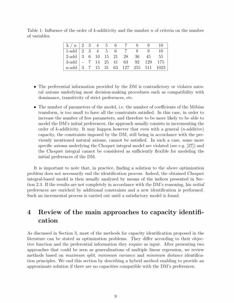
Table 1: Influence of the order of k-additivity and the number n of criteria on the numberof variables.

k / n 2 3 4 5 6 7 8 9 101-add 2 3 4 5 6 7 8 9 102-add 3 6 10 15 21 28 36 45 553-add - 7 14 25 41 63 92 129 175n-add 3 7 15 31 63 127 255 511 1023

• The preferential information provided by the DM is contradictory or violates natu-ral axioms underlying most decision-making procedures such as compatibility withdominance, transitivity of strict preferences, etc.

• The number of parameters of the model, i.e. the number of coefficients of the Mobiustransform, is too small to have all the constraints satisfied. In this case, in order toincrease the number of free parameters, and therefore to be more likely to be able tomodel the DM’s initial preferences, the approach usually consists in incrementing theorder of k-additivity. It may happen however that even with a general (n-additive)capacity, the constraints imposed by the DM, still being in accordance with the pre-viously mentioned natural axioms, cannot be satisfied. In such a case, some morespecific axioms underlying the Choquet integral model are violated (see e.g. [27]) andthe Choquet integral cannot be considered as sufficiently flexible for modeling theinitial preferences of the DM.

It is important to note that, in practice, finding a solution to the above optimizationproblem does not necessarily end the identification process. Indeed, the obtained Choquetintegral-based model is then usually analyzed by means of the indices presented in Sec-tion 2.3. If the results are not completely in accordance with the DM’s reasoning, his initialpreferences are enriched by additional constraints and a new identification is performed.Such an incremental process is carried out until a satisfactory model is found.

4 Review of the main approaches to capacity identifi-

cation

As discussed in Section 3, most of the methods for capacity identification proposed in theliterature can be stated as optimization problems. They differ according to their objec-tive function and the preferential information they require as input. After presenting twoapproaches that could be seen as generalizations of multiple linear regression, we reviewmethods based on maximum split, minimum variance and minimum distance identifica-tion principles. We end this section by describing a hybrid method enabling to provide anapproximate solution if there are no capacities compatible with the DM’s preferences.

9

4.1 Least-squares based approaches

Historically, the first approach that has been proposed can be regarded as a generalization ofclassical multiple linear regression [28]. It requires the additional knowledge of the desiredoverall evaluations y(x) of the available objects x ∈ O. The objective function is defined as

FLS(mν) :=∑

x∈O

[Cmν(u(x)) − y(x)]2 ,

where u(x) := (u1(x1), . . . , un(xn)) for all x ∈ X. The aim is to minimize the averagequadratic distance between the overall utilities {Cmν

(u(x))}x∈O computed by means ofthe Choquet integral and the desired overall scores {y(x)}x∈O provided by the DM. Theoptimization problem takes therefore the form of a quadratic program, not necessarilystrictly convex [29], which implies that the solution, if it exists, is not necessarily unique(this aspect is investigated in detail in [30]). In order to avoid the use of quadratic solvers,heuristic suboptimal versions of this approach have been proposed by Ishii and Sugeno [31],Mori and Murofushi [28] and Grabisch [32]. Let us detail this latter approach.

Called Heuristic Least Mean Squares (HLMS), it is based on a gradient approach startingfrom a DM defined capacity µ that we shall call the initial capacity. This capacity istypically an additive capacity representing the DM’s prior idea of what the aggregationfunction F in Eq. (1) should be. In the absence of clear requirements on the aggregationfunction, a very natural choice for µ is the uniform capacity µ∗ since the Choquet integralw.r.t. that capacity is nothing else than the arithmetic mean. Once the initial capacityµ has been chosen, for each object x ∈ O, the gradient modifies only the coefficients ofµ involved in the computation of Cµ(u(x)) (without violating monotonicity constraints).When all the available objects have been used, unmodified coefficients of µ are modifiedtowards the average value of neighboring coefficients. This forms one iteration, and theprocess is restarted until a stopping criterion is satisfied. The advantage over the optimalquadratic approach is that only the vector of the coefficients of µ has to be stored, whilein the latter, a squared matrix of same dimensions has to be stored. Also, as we shall seein Subsection 5.2, this heuristic approach tends to provide less extreme solutions than theoptimal approach. However, unlike for the optimal quadratic method, it is not possible torequire that the solution be k-additive, k < n.

In the context of MAUT based on the Choquet integral, the main inconvenience of theseapproaches is that they require the knowledge of the desired overall utilities {y(x)}x∈O,which cannot always be obtained from the DM.

4.2 A maximum split approach

An approach based on linear programming was proposed by Marichal and Roubens [33].The proposed identification method can be stated as follows:

10

maxFLP (ε) := ε

subject to

∑

T⊆St≤k−1

mν(T ∪ i) ≥ 0, ∀i ∈ N, ∀S ⊆ N \ i,

∑

T⊆N0<t≤k

mν(T ) = 1,

Cmν(u(x)) − Cmν

(u(x′)) ≥ δC + ε,...

Roughly speaking, the idea of the proposed approach is to maximize the minimal differencebetween the overall utilities of objects that have been ranked by the DM through the partialweak order �O (hence the name maximum split). Indeed, if the DM states that x ≻O x′,he may want the overall utilities to reflect this difference in the most significant way.

The main advantage of this approach is its simplicity. However, as the least squaresbased approach presented in the previous subsection, this identification method does notnecessarily lead to a unique solution, if any. Furthermore, as it will be illustrated inSection 5, the provided solution can sometimes be considered as too extreme, since itcorresponds to a capacity that maximizes the difference between overall utilities.

4.3 Minimum variance and minimum distance approaches

The idea of the minimum variance method [34] is to favor the “least specific” capacity, ifany, compatible with the initial preferences of the DM. The objective function is defined asthe variance of the capacity, i.e.

FMV (mν) :=1

n

∑

i∈N

∑

S⊆N\i

γs(n)

∑

T⊆S

mµ(T ∪ i) −1

n

2

.

As shown in [34], minimizing this variance is equivalent to maximizing the extended Havrdaand Charvat entropy of order 2. This method can therefore be equivalently regarded asa maximum entropy approach. The optimization problem takes the form of the followingstrictly convex quadratic program:

minFMV (mν)

subject to

∑

T⊆St≤k−1

mν(T ∪ i) ≥ 0, ∀i ∈ N, ∀S ⊆ N \ i,

∑

T⊆N0<t≤k

mν(T ) = 1,

Cmν(u(x)) − Cmν

(u(x′)) ≥ δC ,...

As discussed in [34, 35], the Choquet integral w.r.t. the minimum variance capacitycompatible with the initial preferences of the DM, if it exists, is the one that will exploitthe most on average its arguments.

One of the advantages of this approach is that it leads to a unique solution, if any,because of the strict convexity of the objective function. Also, in the case of “poor” initialpreferences involving a small number of constraints, this unique solution will not exhibit too

11

specific behaviors characterized for instance by very high positive or negative interactionindices or a very uneven Shapley value.

A generalization of this approach [36] consists in finding, if it exits, the closest capacityto a capacity defined by the DM and compatible with his/her initial preferences. As alreadydiscussed in Subsection 4.1, this initial capacity is typically an additive capacity representingthe DM’s prior idea of what the aggregation function should be. In the absence of clearrequirements a very natural choice for µ is the uniform capacity µ∗. In order to practicallyimplement such a minimum distance principle, in [36], three quadratic distances have beenstudied. In the sequel, we shall restrict ourselves to the following one defined, for any twogames µ, ν on N by

d2(mµ, mν) :=∫

[0,1]n[Cmν

(x) − Cmµ(x)]2dx. (8)

This quadratic distance, thoroughly studied in [37, Chap. 7] in the context of the exten-sion of pseudo-Boolean functions, can be interpreted as the expected quadratic differencebetween overall utilities computed by Cmµ

and Cmνassuming that the vectors of partial

utilities are uniformly distributed in [0, 1]n.

In the absence of clear requirements on the aggregation function, a natural objectivefunction for the above discussed minimum distance principle is thus given by

FMD(mν) :=∫

[0,1]n

[

Cmν(x) −

1

n

n∑

i=1

xi

]2

dx.

The resulting optimization problem is again a strictly convex quadratic program.

4.4 A less constrained approach

This approach, which is due to Meyer and Roubens [38], can be seen as a generalization ofthe least squares methods described in Subsection 4.1. The minimal preferential informationwhich has to be provided by the DM is a weak order over the available objects. The objectivefunction, depending on more variables than the least squares methods described earlier, isdefined as

FGLS(mν , y) :=∑

x∈O

[Cmν(u(x)) − y(x)]2 ,

where y = {y(x)}x∈O are additional variables of the quadratic program1 representing overallunknown evaluations of the objects that must verify the weak order imposed by the DM.

The optimization problem can be written as the following convex quadratic program :

minFGLS(mν , y)

subject to

∑

T⊆St≤k−1

mν(T ∪ i) ≥ 0, ∀i ∈ N, ∀S ⊆ N \ i,

∑

T⊆N0<t≤k

mν(T ) = 1,

y(x) − y(x′) ≥ δy,...

1The acronym GLS stands for “generalized least squares”.

12

where δy is a indifference threshold, playing a similar role as δC , i.e., it can be interpretedas the desired minimal difference between the overall utilities of two objects which areconsidered as significantly different by the DM. A solution of the quadratic program consistsof the Mobius representation mν of the capacity and the overall evaluations y = {y(x)}x∈O.

Let us first intuitively explain the main idea of the approach. As discussed at the end ofSection 3, assuming that the constraints imposed by the DM are not contradictory and donot question natural multicriteria decision axioms such as compatibility with dominance,it may still happen that the number of parameters (following from the chosen order of k-additivity) is too small so that these constraints can be satisfied. A first possibility consistsin increasing k, if possible. A second solution consists in relaxing some of the constraintsby translating the desired weak order over the available objects by means of conditions onthe unknown overall evaluations {y(x)}x∈O. In that case, the Mobius transform mν is lessconstrained and there may exist a solution.

The role of the objective function is to minimize the quadratic difference between thenumerical representation {y(x)}x∈O of the weak order imposed by the DM and the overallutilities computed by means of the Choquet integral. If the objective function is zero, thenfor each object x, its overall evaluation y(x) equals its aggregated overall utility Cmν

(u(x)).In that case, the weak order obtained by ordering the objects according to their aggregatedevaluations is consistent with the weak order imposed by the DM and the threshold δy is notviolated. Two possibilities arise: either there is a unique solution or there exists an infinityof solutions to the problem. In the second case, the solution is chosen by the solver and itscharacteristics are difficult to predict. If the objective function is strictly positive, then theaggregated overall evaluations {Cmν

(u(x))}x∈O do not exactly match the overall unknownevaluations {y(x)}x∈O numerically representing the weak order imposed by the DM. Twopossibilities arise: either the weak order induced by the aggregated overall evaluations{Cmν

(u(x)}x∈O corresponds to �O but x ≻O x′ does not necessarily imply Cmν(u(x)) ≥

Cmν(u(x′))+δy (see Subsection 5.6), or the weak order induced by the {Cmν

(u(x)}x∈O doesnot correspond to �O. In the former case, the solution does not respect the DM’s choicefor the minimal threshold δy. In the latter case the weak order is violated “on average”which might not be very satisfactory.

The advantage of this approach is that it may provide a solution even if the weak orderover the available objects is incompatible with a Choquet integral model because somespecific axioms are violated (see e.g. [27]), if the indifference threshold δy is too large, or ifsome of the constraints on the criteria are not compatible with a representation of the weakorder by a Choquet integral. It is then on to the DM to decide if the result is satisfactoryor not. Nevertheless, as already explained, this approach should be used with care whenthe objective function is zero, since then, it simply amounts to letting the quadratic solverchoose a feasible solution whose characteristics are difficult to predict.

4.5 Practical implementation

The discussed identification methods have been implemented within the Kappalab pack-age [14] for the GNU R statistical system [15]. The package is distributed as free soft-ware and can be downloaded from the Comprehensive R Archive Network (http://cran.r-project.org) or from http://www.polytech.univ-nantes.fr/kappalab. To solve lin-

13

ear programs, the LpSolve R package [39] is used; strictly convex quadratic programs aresolved using the Quadprog R package [40]; finally, not necessarily strictly convex quadraticprograms are solved using the ipop routine of the Kernlab R package [41].

As far as the maximum number of criteria is considered, Kappalab allows to workcomfortably with up to n = 10 criteria if n-additive capacities are considered and with upto n = 32 criteria if 2 or 3-additive capacities are considered.

5 Applications of the Kappalab R package

5.1 Problem description

We consider an extended version of the fictitious problem presented in [34] concerning theevaluation of students in an institute training econometricians. The students are evaluatedw.r.t. five subjects: statistics (S), probability (P), economics (E), management (M) andEnglish (En). The utilities of seven students a, b, c, d, e, f , g on a [0, 20] scale are given inTable 2.

Table 2: Partial evaluations of the seven students.

Student S P E M En Meana 18 11 11 11 18 13.80b 18 11 18 11 11 13.80c 11 11 18 11 18 13.80d 18 18 11 11 11 13.80e 11 11 18 18 11 13.80f 11 11 18 11 11 12.40g 11 11 11 11 18 12.40

Assume that the institute is slightly more oriented towards statistics and probabilityand suppose that the DM considers that there are 3 groups of subjects: statistics andprobability, economics and management, and English. Furthermore, he/she considers thatwithin the two first groups, subjects are somewhat substitutive, i.e. they overlap to a certainextent. Finally, if a student is good in statistics or probability (resp. bad in statistics andprobability), it is better that he/she is good in English (resp. economics or management)rather than in economics or management (resp. English). This reasoning, applied to theprofiles of Table 2, leads to the following ranking:

a ≻O b ≻O c ≻O d ≻O e ≻O f ≻O g. (9)

We shall further assume that the DM considers that two students are significantly differentif their overall utilities differ by at least half a unit.

By considering students a and b, and f and g, it is easy to see that the criteria do notsatisfy mutual preferential independence, which implies that there is no additive model thatcan numerically represent the above weak order.

14

In order to use the identification methods reviewed in the previous section and imple-mented in Kappalab, we first create 7 R vectors representing the students:

> a <- c(18,11,11,11,18)

> b <- c(18,11,18,11,11)

> c <- c(11,11,18,11,18)

> d <- c(18,18,11,11,11)

> e <- c(11,11,18,18,11)

> f <- c(11,11,18,11,11)

> g <- c(11,11,11,11,18)

The symbol > represents the prompt in the R shell, the symbol <- the assignment operator,and c is the R function for vector creation.

5.2 The least squares approaches

In order to apply the least squares approaches presented in Subsection 4.1, the 7 vectorspreviously defined and representing the students need first to be concatenated into a 7 rowmatrix, called C here, using the rbind (“row bind”) matrix creation function:

> C <- rbind(a,b,c,d,e,f,g)

Then, the DM needs to provide overall utilities for the seven students. Although it is unre-alistic to consider that this information can always be given, we assume in this subsectionthat the DM is able to provide it. He respectively assigns 15, 14.5, 14, 13.5, 13, 12.5 and12 to a, b, c, d, e, f and g. These desired overall utilities are encoded into a 7 element Rvector:

> overall <- c(15,14.5,14,13.5,13,12.5,12)

The least squares identification routine based on quadratic programming (providing anoptimal but not necessarily unique solution) can then be called by typing:

> ls <- least.squares.capa.ident(5,2,C,overall)

in the R terminal. The first argument sets the number of criteria, the second fixes the desiredorder of k-additivity, and the two last represent the matrix containing the partial utilitiesand the vector containing the desired overall utilities respectively. The result is stored inan R list object, called here ls, containing all the relevant information for analyzing theresults.

The solution, a 2-additive capacity given under the form of its Mobius representation,can be obtained by typing:

> m <- ls$solution

and visualized by entering m in the R terminal:

15

> m

Mobius.capacity

{} 0.000000

{1} 0.311650

{2} 0.176033

... ...

{4,5} 0.001752

As discussed in Subsection 4.1, for the considered example, the obtained solution is probablynot unique [30].

The Choquet integral for instance of a w.r.t. the solution can be obtained by typing:

> Choquet.integral(m,a)

[1] 15

To use the least squares identification routine implementing the heuristic approach pro-posed in [32], we first need to create the initial capacity as discussed in Subsection 4.1.Here, in the absence of clear requirements on the form of the Choquet integral, we take theuniform capacity on the set of criteria (subjects):

> mu.unif <- as.capacity(uniform.capacity(5))

The heuristic least squares identification routine can then be called by typing:

> hls <- heuristic.ls.capa.ident(5,mu.unif,C,overall,alpha=0.05)

The first argument sets the number of criteria, the second contains the initial capacity, thethird represents the matrix of the partial evaluations, the fourth the vector containing thedesired overall utilities, and the last the value of the parameter controlling the gradientdescent.

The overall utilities computed using the Choquet integral w.r.t. the two obtained solu-tions are given in the last two columns of the table below, the sixth column containing thedesired overall evaluations:

S P E M En Given Mean LS HLS

a 18 11 11 11 18 15.0 13.8 15.0 15.0

b 18 11 18 11 11 14.5 13.8 14.5 14.5

c 11 11 18 11 18 14.0 13.8 14.0 14.0

d 18 18 11 11 11 13.5 13.8 13.5 13.5

e 11 11 18 18 11 13.0 13.8 13.0 13.0

f 11 11 18 11 11 12.5 12.4 12.5 12.5

g 11 11 11 11 18 12.0 12.4 12.0 12.0

As one can see, both the optimal and the heuristic approaches enable to recover the overallutilities provided by the DM. Recall however that the solution returned by the optimalquadratic method is 2-additive whereas that returned by the heuristic method is 5-additive.

The Shapley values of the solutions can be computed by means of the Shapley.value

function taking as argument a capacity and are given in the following table :

16

S P E M En

LS 0.29 0.14 0.21 0.13 0.24

HLS 0.24 0.18 0.20 0.16 0.21

As one could have expected, the Shapley value of the solution obtained by the heuristicapproach is more even than that returned by the optimal quadratic method.

5.3 The LP, minimum variance and minimum distance approaches

As discussed earlier, the least squares approaches applied in the previous subsection are notwell adapted to MAUT since they rely on information that a DM cannot always provide.The LP, the minimum variance and the minimum distance approaches require only a partialweak order over the available objects, such as the one provided by the DM in Eq. (9). Thisweak order is naturally translated as

Cmν(a) > Cmν

(b) > Cmν(c) > Cmν

(d) > Cmν(e) > Cmν

(f) > Cmν(g).

with indifference threshold δC = 0.5.

Practically, the preference threshold is stored in an R variable:

> delta.C <- 0.5

and the weak order over the students is encoded into a 6 row R matrix:

> Acp <- rbind(c(a,b,delta.C), c(b,c,delta.C), c(c,d,delta.C),

c(d,e,delta.C), c(e,f,delta.C), c(f,g,delta.C))

each row containing a constraint of the form Cmν(u(x)) ≥ Cmν

(u(y)) + δC .

The LP approach is then invoked by typing:

> lp <- lin.prog.capa.ident(5,2,A.Choquet.preorder = Acp)

The first argument fixes the number of criteria, the second sets the desired order of k-additivity for the solution, and the last contains the partial weak order provided by theDM. All the relevant information to analyze the solution is stored in the R object lp.

The minimum variance approach is called similarly:

> mv <- mini.var.capa.ident(5,2,A.Choquet.preorder = Acp)

To use the minimum distance approach, we first need to create the initial capacity. Inthe absence of clear requirements from the DM, we choose the uniform capacity on the setof criteria (subjects), which can be created by entering:

> m.mu <- additive.capacity(c(0.2,0.2,0.2,0.2,0.2))

The closest capacity to the uniform capacity compatible with the initial preferences of theDM is then obtained by typing:

17

> md <- mini.dist.capa.ident(m.mu,2,"global.scores",

A.Choquet.preorder = Acp)

The second argument sets the desired order of k-additivity for the solution, while the thirdone indicates which of the 3 available quadratic distances between capacities should beused [36]. The character string "global.scores" refers to the distance given in Eq. (8).

The overall utilities computed using the Choquet integral w.r.t. the 2-additive solutionsare given in the following table:

S P E M En Mean LP MV MD

a 18 11 11 11 18 13.8 18.00 15.25 14.95

b 18 11 18 11 11 13.8 17.36 14.75 14.45

c 11 11 18 11 18 13.8 16.73 14.25 13.95

d 18 18 11 11 11 13.8 16.09 13.75 13.45

e 11 11 18 18 11 13.8 15.45 13.25 12.95

f 11 11 18 11 11 12.4 14.82 12.75 12.45

g 11 11 11 11 18 12.4 14.18 12.25 11.95

Note that, as expected, the LP approach leads to more dispersed utilities, which reachthe maximum value (18) that a Choquet integral can take for the seven students. Notealso that, for the minimum variance and the minimum distance approaches, the differencesbetween the overall utilities of two consecutive students in the weak order provided by theDM equal exactly δC . This last observation follows from the fact that, in this example, theaim of both methods is roughly to find the Choquet integral that is the closest to the simplearithmetic mean while being in accordance with the preferential information provided bythe DM.

The Shapley values of the 2-additive solutions are:

S P E M En

LP 0.45 0.00 0.27 0.05 0.23

MV 0.27 0.16 0.21 0.14 0.22

MD 0.24 0.18 0.20 0.16 0.22

As one can see, all three solutions designate statistics (S) as the most important criterion.Note that the LP solution is very extreme, since the overall importance of probability (P)and management (M) is very small and that of S is close to one half.

However, the overall importances of the criteria are not in accordance with the orienta-tion of the institution. Indeed, one would have expected to obtain that statistics (S) andprobability (P), and economics (E) and management (M), have the same importances. Thisis due to the fact that until now, the preferential information which we used was limited toa small number of students which were ranked by the DM. In order to build a more accuratemodel, we can impose additional constraints as we shall see in the next subsection. Thisclearly justifies the use of a progressive interactive approach to model the DM’s preferencesin MAUT.

18

5.4 Additional constraints on the Shapley value

As discussed in the previous subsection, assume now that by considering the Shapley val-ues of the 2-additive solutions obtained above, the DM explicitly requires that statistics(S) and probability (P), and economics (E) and management (M), have the same overallimportances, i.e. S ∼N P and E ∼N M .

These additional constraints are translated as −δφ ≤ φmν(S)−φmν

(P ) ≤ δφ and −δφ ≤φmν

(E) − φmν(M) ≤ δφ, where the indifference threshold δφ is supposed to have been set

to 0.01 by the DM. To encode them, an R variable representing the indifference thresholdis first created:

> delta.phi <- 0.01

The inequalities discussed above are then encoded into a 4 row R matrix:

> Asp <- rbind(c(1,2,-delta.phi), c(2,1,-delta.phi),

c(3,4,-delta.phi), c(4,3,-delta.phi))

each row corresponding to a constraint of the form φmν(i) − φmν

(j) ≥ c, c ∈ [0, 1].

The LP approach is then invoked by typing

> lp2 <- lin.prog.capa.ident(5,2,A.Choquet.preorder = Acp,

A.Shapley.preorder = Asp)

into the R terminal. The minimum variance and minimum distance routines are calledsimilarly.

The Shapley values of the 2-additive solutions are:

S P E M En

LP 0.23 0.23 0.18 0.18 0.18

MV 0.22 0.21 0.18 0.17 0.22

MD 0.22 0.21 0.18 0.17 0.22

As expected, the solutions satisfy the constraints additionally imposed by the DM.

The overall utilities computed using the Choquet integral w.r.t. the 2-additive solutionsare given in the following table:

S P E M En Mean LP MV MD

a 18 11 11 11 18 13.8 16.03 15.12 14.84

b 18 11 18 11 11 13.8 15.52 14.62 14.34

c 11 11 18 11 18 13.8 15.01 14.12 13.84

d 18 18 11 11 11 13.8 14.50 13.62 13.34

e 11 11 18 18 11 13.8 13.99 13.12 12.84

f 18 18 11 11 11 12.4 13.48 12.62 12.34

g 11 11 18 11 11 12.4 12.97 12.12 11.84

19

This time, the three approaches give more similar overall utilities. This was to be expectedas the problem is more constrained.

The interaction indices of the 2-additive capacities obtained by means of the LP, mini-mum variance and minimum distance approaches are respectively given in the three tablesbelow:

[LP] S P E M En

S NA -0.27 -0.17 0.00 -0.03

P -0.27 NA 0.00 0.16 -0.04

E -0.17 0.00 NA -0.12 -0.06

M 0.00 0.16 -0.12 NA -0.07

En -0.03 -0.04 -0.06 -0.07 NA

[MV] S P E M En

S NA -0.21 -0.05 -0.06 0.10

P -0.21 NA 0.01 0.15 -0.03

E -0.05 0.01 NA -0.12 0.05

M -0.06 0.15 -0.12 NA -0.01

En 0.10 -0.03 0.05 -0.01 NA

[MD] S P E M En

S NA -0.21 -0.04 -0.07 0.10

P -0.21 NA 0.03 0.18 -0.01

E -0.04 0.03 NA -0.10 0.09

M -0.07 0.18 -0.10 NA 0.00

En 0.10 -0.01 0.09 0.00 NA

As one can notice, statistics (S) negatively interacts with almost all the subjects, whichagain is not in accordance with the orientation of the institution. Indeed, one would expectstatistics (S) to be complementary with all subjects except probability (P). Once more, inthe perspective of a progressive and interactive approach, this can be corrected by imposingadditional constraints on the interaction indices as we shall see in the next subsection.

5.5 Additional constraints on the interaction indices

Assume finally that, in order to be in accordance with the orientation of the institution, theDM imposes that subjects within the same group2 have to interact in a substitutive way,whereas two subjects from different groups have to interact in a complementary way. Thisadditional preferential information is translated by means of the following constraints:

P E M En

−1 ≤ Imν (SP ) ≤ −δI δI ≤ Imν (SE) ≤ 1 δI ≤ Imν (SM) ≤ 1 δI ≤ Imν (SEn) ≤ 1 SδI ≤ Imν (PE) ≤ 1 δI ≤ Imν (PM) ≤ 1 δI ≤ Imν (PEn) ≤ 1 P

−1 ≤ Imν (EM) ≤ −δI δI ≤ Imν (EEn) ≤ 1 EδI ≤ Imν (MEn) ≤ 1 M

where δI , supposed set to 0.05, is a DM defined threshold to be interpreted as the minimalabsolute value of an interaction index to be considered as significantly different from zero.

To encode this additional preferential information, an R variable representing the thresh-old is first created:

> delta.I <- 0.05

2Recall that the three groups of subjects are {S, P}, {E,M}, and {En}.

20

The constraints discussed above are then encoded into a 10 row R matrix:

> Aii <- rbind(c(1,2,-1,-delta.I), c(1,3,delta.I,1), c(1,4,delta.I,1),

c(1,5,delta.I,1), c(2,3,delta.I,1), c(2,4,delta.I,1),

c(2,5,delta.I,1), c(3,4,-1,-delta.I), c(3,5,delta.I,1),

c(4,5,delta.I,1))

each row corresponding to a constraint of the form a ≤ Imν(ij) ≤ b, a, b ∈ [−1, 1].

There are no 2-additive capacities compatible with these additional constraints. Theorder of k-additivity is then incremented and the LP approach is invoked by typing:

> lp3 <- lin.prog.capa.ident(5,3, A.Choquet.preorder = Acp,

A.Shapley.preorder = Asp,

A.interaction.interval = Aii)

The minimum variance and minimum distance routines are called similarly.

The Shapley values and the interaction indices of the three 3-additive solutions are givenin the four following tables:

S P E M En

LP 0.23 0.23 0.16 0.16 0.22

MV 0.23 0.22 0.18 0.18 0.20

MD 0.22 0.21 0.18 0.19 0.21

[LP] S P E M En

S NA -0.30 0.05 0.05 0.12

P -0.30 NA 0.07 0.14 0.05

E 0.05 0.07 NA -0.24 0.05

M 0.05 0.14 -0.24 NA 0.05

En 0.12 0.05 0.05 0.05 NA

[MV] S P E M En

S NA -0.13 0.05 0.05 0.05

P -0.13 NA 0.05 0.05 0.05

E 0.05 0.05 NA -0.05 0.05

M 0.05 0.05 -0.05 NA 0.05

En 0.05 0.05 0.05 0.05 NA

[MD] S P E M En

S NA -0.21 0.05 0.05 0.05

P -0.21 NA 0.05 0.05 0.05

E 0.05 0.05 NA -0.12 0.05

M 0.05 0.05 -0.12 NA 0.05

En 0.05 0.05 0.05 0.05 NA

As expected, the constraints additionally imposed by the DM are satisfied.

The overall utilities computed using the Choquet integral w.r.t. the 3-additive solutionsare given in the following table:

S P E M En Mean LP MV MD

a 18 11 11 11 18 13.8 14.06 14.26 14.45

b 18 11 18 11 11 13.8 13.55 13.76 13.95

c 11 11 18 11 18 13.8 13.04 13.26 13.45

d 18 18 11 11 11 13.8 12.53 12.76 12.95

e 11 11 18 18 11 13.8 12.02 12.26 12.45

f 18 18 11 11 11 12.4 11.51 11.76 11.95

g 11 11 18 11 11 12.4 11.00 11.26 11.45

We hereby conclude the process of the modeling of the DM’s preferences. In the followingsection we imagine a scenario where the DM considers that the 3-additive solutions aboveare too complex and where he/she prefers to have a simpler description of his preferences.In such a case, the DM has to take into account that some of his preferences will be violated.

21

5.6 A simpler solution

Assume that for the sake of simplicity the DM absolutely wants a 2-additive solution forthe problem described in the previous subsections. In that case, it is possible to use thegeneralized least squares approach described in Subsection 4.4 to obtain an approximatesolution.

First of all, the weak order over the students has to be encoded into a 6 row R matrix:

> rk.proto <- rbind(c(1,2), c(2,3), c(3,4), c(4,5), c(5,6), c(6,7))

The integers correspond to the line indices of the alternatives a, b, c, d, e, f and g in thematrix C defined in Subsection 5.2.

The generalized least squares approach can then be called by typing:

> gls <- ls.ranking.capa.ident(5, 2, C, rk.proto, 0.5,

A.Shapley.preorder = Asp,

A.interaction.interval = Aii)

The first argument sets the number of criteria, the second the desired order of k-additivity,the third the matrix containing the partial evaluations, the fourth the matrix containing theweak order and the fifth argument is the value of the threshold δy. The two last argumentscontain the matrices encoding the additional constraints on the Shapley value and on theinteraction indices respectively.

Although we know from the previous subsections that there are no 2-additive capacitiescompatible with the imposed constraints, this approach provides a solution with a non zeroobjective function as we could have expected. The following table gives the aggregatedoverall utilities {Cmν

(u(x))}x∈O in the last column and the overall utilities {y(x)}x∈O inthe last but one column:

S P E M En Mean y GLS

a 18 11 11 11 18 13.8 13.94 13.67

b 18 11 18 11 11 13.8 13.44 13.44

c 11 11 18 11 18 13.8 12.94 12.81

d 18 18 11 11 11 13.8 12.44 12.57

e 11 11 18 18 11 13.8 11.94 11.81

f 18 18 11 11 11 12.4 11.44 11.57

g 11 11 18 11 11 12.4 10.94 11.21

As one can see, the ranking provided by the DM is not violated but the minimal thresholdδy is not always respected (for example Cmν

(f)−Cmν(g) < δy). The Shapley value and the

interaction indices of this 2-additive solution are:

S P E M En

0.23 0.22 0.17 0.16 0.22

S P E M En

S NA -0.22 0.05 0.05 0.14

P -0.22 NA 0.06 0.09 0.06

E 0.05 0.06 NA -0.08 0.15

M 0.05 0.09 -0.08 NA 0.05

En 0.14 0.06 0.15 0.05 NA

22

which as expected satisfy the constraints imposed by the DM. It is now up to the DMto evaluate if the violation of δy does not deteriorate significantly the overall quality of themodel.

References

[1] R. L. Keeney and H. Raiffa. Decision with multiple objectives. Wiley, New-York, 1976.

[2] D. Bouyssou and M. Pirlot. Conjoint measurement tools for MCDM: A brief intro-duction. In J. Figuera, S. Greco, and M. Ehrgott, editors, Multiple Criteria DecisionAnalysis: State of the Art Surveys, pages 73–132. Springer, 2005.

[3] D.H. Krantz, R.D. Luce, P. Suppes, and A. Tversky. Foundations of measurement,volume 1: Additive and polynomial representations. Academic Press, 1971.

[4] D. Bouyssou and M. Pirlot. Preferences for multi-attributed alternatives: Traces,dominance, and numerical representations. J. of Mathematical Psychology, 48:167–185, 2004.

[5] P. Vincke. Multicriteria Decision-aid. Wiley, 1992.

[6] G. Choquet. Theory of capacities. Annales de l’Institut Fourier, 5:131–295, 1953.

[7] M. Sugeno. Theory of fuzzy integrals and its applications. PhD thesis, Tokyo Instituteof Technology, Tokyo, Japan, 1974.

[8] M. Grabisch. The application of fuzzy integrals in multicriteria decision making. Eu-ropean Journal of Operational Research, 89:445–456, 1992.

[9] J.-L. Marichal. An axiomatic approach of the discrete Choquet integral as a tool toaggregate interacting criteria. IEEE Transactions on Fuzzy Systems, 8(6):800–807,2000.

[10] C. Labreuche and M. Grabisch. The Choquet integral for the aggregation of intervalscales in multicriteria decision making. Fuzzy Sets and Systems, 137:11–16, 2003.

[11] M. Grabisch, Ch. Labreuche, and J.C. Vansnick. On the extension of pseudo-Booleanfunctions for the aggregation of interacting criteria. European Journal of OperationalResearch, 148:28–47, 2003.

[12] C.A. Bana e Costa and J.C. Vansnick. Preference relations in MCDM. In T. Gal andT. Hanne T. Steward, editors, MultiCriteria Decision Making: Advances in MCDMmodels, algorithms, theory and applications. Kluwer, 1999.

[13] M. Grabisch and C. Labreuche. Fuzzy measures and integrals in MCDA. In J. Figueira,S. Greco, and M. Ehrgott, editors, Multiple Criteria Decision Analysis, pages 563–608.Springer, 2004.

[14] M. Grabisch, I. Kojadinovic, and P. Meyer. kappalab: Non additive measure andintegral manipulation functions, 2006. R package version 0.3.

23

[15] R Development Core Team. R: A language and environment for statistical computing.R Foundation for Statistical Computing, Vienna, Austria, 2005. ISBN 3-900051-00-3.

[16] T. Murofushi and M. Sugeno. Fuzzy measures and fuzzy integrals. In M. Grabisch,T. Murofushi, and M. Sugeno, editors, Fuzzy Measures and Integrals: Theory andApplications, pages 3–41. Physica-Verlag, 2000.

[17] D. Schmeidler. Subjective probability and expected utility without additivity. Econo-metrica, 57(3):571–587, 1989.

[18] G-C. Rota. On the foundations of combinatorial theory. I. Theory of Mobius functions.Z. Wahrscheinlichkeitstheorie und Verw. Gebiete, 2:340–368 (1964), 1964.

[19] A. Chateauneuf and J-Y. Jaffray. Some characterizations of lower probabilities andother monotone capacities through the use of Mobius inversion. Mathematical SocialSciences, 17(3):263–283, 1989.

[20] J.-L. Marichal. Behavioral analysis of aggregation in multicriteria decision aid. InJ. Fodor, B. De Baets, and P. Perny, editors, Preferences and Decisions under Incom-plete Knowledge, pages 153–178. Physica-Verlag, 2000.

[21] J-L. Marichal. Tolerant or intolerant character of interacting criteria in aggregationby the Choquet integral. European Journal of Operational Research, 155(3):771–791,2004.

[22] L. S. Shapley. A value for n-person games. In Contributions to the theory of games,vol. 2, Annals of Mathematics Studies, no. 28, pages 307–317. Princeton UniversityPress, Princeton, N. J., 1953.

[23] M. Grabisch and Marc Roubens. An axiomatic approach to the concept of interactionamong players in cooperative games. Internat. J. Game Theory, 28(4):547–565, 1999.

[24] T. Murofushi and S. Soneda. Techniques for reading fuzzy measures (iii): Interactionindex. In 9th Fuzzy System Symposium, pages 693–696, Saporo, Japan, 1993.

[25] M. Grabisch. k-order additive discrete fuzzy measures and their representation. FuzzySets and Systems, 92(2):167–189, 1997.

[26] K. Fujimoto, I. Kojadinovic, and J-L. Marichal. Axiomatic characterizations of proba-bilistic and cardinal-probabilistic interaction indices. Games and Economic Behavior,55:72–99, 2006.

[27] P. Wakker. Additive Representations of Preferences: A New Foundation of DecisionAnalysis. Kluwer Academic Publishers, Dordrecht, 1989.

[28] T. Mori and T. Murofushi. An analysis of evaluation model using fuzzy measure andthe Choquet integral. In 5th Fuzzy System Symposium, pages 207–212, Kobe, Japan,1989. In Japanese.

[29] M. Grabisch, H.T. Nguyen, and E.A. Walker. Fundamentals of uncertainty calculi withapplications to fuzzy inference. Kluwer Academic, Dordrecht, 1995.

24

[30] P. Miranda and M. Grabisch. Optimization issues for fuzzy measures. Int. J. ofUncertainty, Fuzziness, and Knowledge Based Systems, 7:545–560, 1999.

[31] K. Ishii and M. Sugeno. A model of human evaluation process using fuzzy measure.Int. J. Man-Machine Studies, 67:242–257, 1996.

[32] M. Grabisch. A new algorithm for identyfing fuzzy measures and its application to pat-tern recognition. In Int. 4th IEEE Conf. on Fuzzy Systems, pages 145–150, Yokohama,Japan, March 1995.

[33] J-L. Marichal and M. Roubens. Determination of weights of interacting criteria froma reference set. European Journal of Operational Research, 124:641–650, 2000.

[34] I. Kojadinovic. Minimum variance capacity identification. European Journal of Oper-ational Research, 177(1):498–514, 2007.

[35] I. Kojadinovic, J-L. Marichal, and M. Roubens. An axiomatic approach to the defini-tion of the entropy of a discrete Choquet capacity. Information Sciences, 172:131–153,2005.

[36] I. Kojadinovic. Quadratic distances for capacity and bi-capacity approximation andidentification. 4OR: A Quarterly Journal of Operations Research, page in press, 2006.

[37] J-L. Marichal. Aggregation operators for multicriteria decison aid. PhD thesis, Uni-versity of Liege, Liege, Belgium, 1998.

[38] P. Meyer and M. Roubens. Choice, ranking and sorting in fuzzy Multiple CriteriaDecision Aid. In J. Figueira, S. Greco, and M. Ehrgott, editors, Multiple CriteriaDecision Analysis: State of the Art Surveys, pages 471–506. Springer, New York, 2005.

[39] Michel Berkelaar et al. lpSolve: Interface to LPSolve v.5 to solve linear/integerprograms, 2005. R package version 1.1.9.

[40] B.A. Turlach and A. Weingessel. quadprog: Functions to solve quadratic programmingproblems., 2004. R package version 1.4-7.

[41] Alexandros Karatzoglou, Alex Smola, Kurt Hornik, and Achim Zeileis. kernlab: AnS4 package for kernel methods in R. Journal of Statistical Software, 11(9):1–20, 2004.

25