A Review of Regression Diagnostics - Conservancy - University of

209

A Review of Regression Diagnosticsfor Behavioral Research

Sangit Chatterjee and Mustafa YilmazNortheastern University

Influential data points can affect the results ofa regression analysis; for example, the usual sum-mary statistics and tests of significance may bemisleading. The importance of regressiondiagnostics in detecting influential points isdiscussed, and five statistics are recommended forthe applied researcher. The suggested diagnosticswere used on a small dataset to detect an influen-tial data point, and the effects were analyzed.Colinearity-based diagnostics also are discussedand illustrated on the same dataset. The non-robustness of the least squares estimates in thepresence of influential points is emphasized.Diagnostics for multiple influential points, multi-variate regression, multicolinearity, nonlinearregression, and other multivariate procedures alsoare discussed. Index terms: Andrew-Pregibonmeasure, colinearity, Cook’s distance, covarianceratio, influential observations, measurement error,partial residual plot, regression diagnostics.

Explanation of the relationships among vari-ables is a major goal of the behavioral and socialsciences. To achieve this goal, relevant variablesand constructs must be discovered and measuredon reasonably precise scales. Because many be-havioral variables do not lend themselves to ex-act measurement, establishment of reliable andvalid measures for these variables is a continuingchallenge facing behavioral scientists.Common approaches to the study of relation-

ships among variables include correlation andregression models. For these models to be useful,the variables must be measured with as little erroras possible because errors in measurement tendto attenuate or distort the relationships among

variables, which causes serious difficulties in theinterpretation of results. Consequently, avoidingadditional distortions that arise from influentialdata points and outliers gains added importancein the use of these models in the behavioralsciences.

Observed variables include errors only whena model can be specified for the variables thatdistinguishes between underlying unobservableand observable components of measurementerrors. Regression models have extensive psycho-metric problems. For example, Lord & Novick

(1968) and Nunnally (1967) include in-depthdiscussions of corrections for attenuation, restric-tion of range, unreliability, measurement errors,and other errors. Although awareness of the psy-chometric problems is vital, it is also importantto recognize the estimation bias arising fromdiscrepant data points and the important role thatdiagnostics play in uncovering such points.Although the concern here is less with the psy-chometric issues and more with the study ofregression diagnostics, an integrative approach isused because problems such as measurementerrors are common to both concerns. Only a fullunderstanding of the importance of both kindsof issues can lead to acceptable models for thesocial and behavioral sciences.

The importance of influential data points andoutliers on estimates calculated in a linear regres-sion model has generated such a large body ofwork that a new subfield-regression diagnos-tics-has developed. With some recent exceptionsnoted below, this work has received little atten-tion in statistical analysis books used by socialscientists or in social science journals. For ex-

Downloaded from the Digital Conservancy at the University of Minnesota, http://purl.umn.edu/93227. May be reproduced with no cost by students and faculty for academic use. Non-academic reproduction

requires payment of royalties through the Copyright Clearance Center, http://www.copyright.com/

210

ample, Pedhazur (1982) only briefly discussesoutliers and influential points, even thoughpopular statistical software provides several

diagnostics [e.g., BMDP (Dixon, 1984), MINITAB(Ryan, Joiner, & Ryan, 1991), SAS (SAS Institute,Inc., 1982), SPSS (SPSS Inc., 1988), and SYSTAT(Wilkinson, 1992)].

Recent reviews somewhat narrower in scopethan this review include Cook & Weisberg(1982b), Stevens (1984), and Bollen & Jackman

(1985). Most recent applied statistics books (e.g.,Darlington, 1990) also contain at least somediscussion of regression diagnostics. Specializedbooks by Chatterjee & Hadi (1988), Atkinson(1985), Cook & Weisberg (1982a), and Belsley,Kuh, & Welsch (1980) deal exclusively with regres-sion diagnostics, influential observations, andoutliers. For useful and substantive applicationsof regression diagnostics in the social sciences,see Bollen & Jackman (1985) and Chatterjee &Wiseman (1984). The present paper is intendedto be broader in scope and less technical in its

presentation. The concepts behind the statisticsare emphasized at the cost of mathematical rigor.Formal tests of hypotheses are not emphasized,because regression diagnostics are intended asexploratory data analysis.

Regression Models

This paper considers the general linear regres-sion model,

or y xo + ~ F, in matrix notation, where

y = (y¡, ... , yet is a n x I column vector ofrc observations of a stochastic response (depen-dent or criterion) variable y, and T denotes thetranspose. For the ith observation, x;&dquo; x,2, ... ,

xi, are the observed values of k regressor (in-dependent or predictor) variables X,, X,, ... , I Xil.P = (P., ... , Bk)T is a (k + 1) x 1 column vec-tor of unknown constants, £ = (E~ , ..., EnY isa aa x 1 column vector of random errors, and xis a rc X (k + 1) matrix with its first column con-sisting of Is, and the remaining columns contain-

ing the regressor values x;;, i = 1, 2, ..., n and

j = 1, 2, ..., k. As usual, the ordinary leastsquares (ALS) estimates are denoted by b = (b~,- - . , ~)~, given by b = (XTX)-IXTy, which is ob-tained by minimizing ZTZ with respect to (3. It isassumed that the random errors Fi are indepen-dent with mean 0 and variance cr2 (homoscedas-ticity). If the xiis can be regarded as fixed con-stants, then the OLS estimates are optimal in thesense of being unbiased and having minimumvariance among all linear estimators (i.e., the bestlinear unbiased estimator). The estimates of theslopes are given by bp b2, ... , bk; the estimateof the standard error of the regression equation02 is given by

and the measure of fit by

where y is the fitted value. The adjusted RZ valueis given by

For purposes of inference beyond point estima-tion, such as tests of hypotheses, errors are oftenassumed to be normally distributed.

If either assumption-homoscedasticity or in-dependence of errors-is not tenable, it is still

theoretically possible to obtain optimal estimatesof the flys using generalized least squares estima-tion, which minimizes ~T~-’~, where ~ is then x n variance-covariance matrix of s. If theobserved values of the regressors are regarded asfixed constants, then the values of the regressorsshould be fixed prior to sampling, and repeatedobservations of the response variable should bemade only for these fixed values of the regressors.

In most behavioral studies, it is not feasibleor appropriate to conduct experiments by fixingthe regressors as known constants. Fortunately,the linear model and its estimation remain essen-

tially unchanged if the conditional distributions



211

of the yi, given x = lxijl, are independent withconstant variance a2, and regressors are indepen-dent random variables with distributions that donot depend on the parameters [3 or the constantvariance o~. Even correlated errors present no ad-ditional problems if it can be assumed that thedistribution of x does not depend on [3 or E.

Because the true values of these parameters areunknown, sample estimates provide the onlyadequate means of testing the validity of theseassumptions in practice. This is usually achievedby examining plots of residuals (the observedvalue minus the fitted value) resulting from anestimated model, such as the plots of residualsagainst the predicted response or against eachregressor variable. If the assumptions are not met,however, parameter estimates obtained from OLSeither will be biased or have other non-optimalproperties (such as lack of consistency). Leastsquares estimates will be nonoptimal, for ex-ample, if the regressor variables are stochastic butare correlated with the errors.

If the distributional assumptions stated aboveare not met for the stochastic variables, a sug-gested alternative to OLS estimation involves

searching for additional variables that can be usedto model the regressor variables and that satisfythe usual assumptions. These lead to two-stageleast squares estimation and linear structural equa-tions models that are outside the scope of the pres-ent review (see, e.g., Bollen, 1989; Judge, Griffith,Hill, & Lee, 1980; Malinvaud, 1970).

Models With Measurement Error

Errors in measuring the response variable y donot require any special attention, because theseerrors are absorbed in the random errors of the

regression model. Thus, the net effect of errorsin y is a larger standard error of the estimatedregression coefficients. On the other hand,measurement errors in regressor variables pro-duce error terms that are correlated with the

regressors. Measurement error may affect statis-tical analysis because it can cause the probabilitydistribution of observed data to differ from thedistribution of the error-free data [see Cochran

(1972), Stefanski (1985), and Chesher (1991) forinformation on measurement error models]. Asnoted above, the presence of measurement errorleads to estimates of the regression coefficientsthat are nonoptimal (i.e., biased or inconsistent).The effect of this nonoptimality can be inves-tigated using (1) the asymptotic approach, (2) theperturbation approach, and (3) the simulationapproach.

In the asymptotic approach, which is popularin econometrics, large sample biases are

calculated analytically and limiting values aresought (Chatterjee & Hadi, 1986). In the pertur-bation approach, the effects on the regressioncoefficients of perturbing the regressors by smallamounts are studied analytically. This methodprovides an upper bound on the relative errorsin the estimated coefficients (see Stewart, 1987).In the simulation approach, the structure of theerrors in the regressor variables is simulated, andthe effects are studied on the estimated regres-sion coefficients (Chatterjee & Hadi, 1986).These three approaches require the researcher tomake assumptions about the form of the distribu-tions, the moments of the distributions, and/orthe bounds on the errors in the variables. Referto Chatterjee & Hadi (1988) for details of all threemethods. Fuller (1987) and Heller (1987) provid-ed specialized discussions for studying variousaspects of measurement errors on the parameterestimates, and Bollen (1989) discussed modelingin the presence of these errors.

In theory, &dquo;instrumental variables&dquo; may pro-vide a possible solution to the problem ofmeasurement errors in the regression variables.Instrumental variables correlate very highly withthe regressors but not with the measurementerrors in the regressors or the random errorsassociated with the dependent variable. If suchvariables can be found, they can be used asregressor variables; alternatively, regressorvariables could be modeled in terms of the in-strumental variables. This last approach leads tothe estimation of simultaneous equations by thetwo-stage least squares approach mentionedabove (Judge et al., 1980). Clearly, the main



212

problems with this approach are identifying theinstrumental variables and collecting data forthem. When measurement errors are of concern,the researcher must decide on a strategy for deal-

ing with them before using regression diagnostics.

Cross-Validation

Regression diagnostics are useful for detectinginfluential observations and may help the userselect the proper statistical model. Cross-

validation is another technique used in the socialsciences to test the appropriateness of a modelfor a given set of observations. In cross-

validation, a portion of the data is not used indeveloping the regression model (Picard & Berk,1990; Picard & Cook, 1984). Three different waysto conduct cross-validation are suggested in theliterature: (1) the split-sample method, (2) thehold-out method, and (3) the leave-one-out orjackknife method.

The first two approaches are very similar

techniques in that they are both simple and in-tuitively appealing. In the split-sample method,50% of the observations are used for estimation,and the remaining 50% are used for the valida-tion of the model under consideration. This pro-cedure may result in inefficient and/or inaccurateestimation and validation if the total number ofobservations is not large. In the hold-out method,a larger portion (e.g., 80%) of the data are usedfor estimation, and a smaller portion (e.g., 20%)are used for validation. The rationale for holdingout a larger portion of the observations is thatthe accuracy of the cross-validation cannot be

judged without precise estimates. However, evenwith this method, a small sample might result inimprecise estimation.

The jackknife method is an attempt to com-bine the strengths of the above two methods. Theregression model is estimated with (n - 1) obser-vations, and the observation which is left out ispredicted from the regression model obtainedfrom the (n - 1) observations. This process is

repeated by bringing in the previously left outobservation and leaving out a different observa-tion. Thus, ~a predictions are obtained that can

be used to judge the efficacy of the model. Inthis case, a balance is reached for both estima-tion and prediction. This idea also appears insome regression diagnostics, such as the ex-

ternally studentized residual.

Influential Observations and

Regression DiagnosticsA distinction must be made between outliers

and influential points. Outliers are unusually ex-treme values in the response variable. Influential

variables are extreme values in regressor variablesthat have a disproportionate effect on parameterestimates such as the slope, estimated standarderror of the regression equation, R2, and soforth. Because each point in a regression spaceis defined by a combination of a response vari-able and a regressor variable, outliers may or maynot be influential observations and influentialvariables may or may not be outliers. Figure I

illustrates this in the context of a bivariate linear

regression. In Figure la, A’ is an outlier but notan influential data point; if A’ is shifted to posi-tion A&dquo;, it becomes an influential point and notan outlier. In Figure lb, A’ is an influential pointbut not an outlier. If A’ is moved to position A&dquo;,then it continues to be an influential point butalso becomes an outlier. In the context of multi-

ple regression, simple two-dimensional scatterplots cannot be used and the value of diagnosticsbecomes apparent.

If influential points are present, serious errorsmay be made in interpreting the regression model.In extreme cases, it is possible to conclude thata hypothesized relationship exists when in factit does not, or to conclude that no relationshipexists when it does. In Figure lc, point A is highlyinfluential-the regression line has a positiveslope when A is included, but it has a horizontalline indicating no relationship when A is exclud-ed. In Figure Id, the inclusion of the influentialpoint A yields a horizontal regression line,whereas its exclusion gives a line having positiveslope.

Point A in Figure lc is no longer an influen-tial point if a curvilinear model is used. Thus,



213

Figure 1Examples of Outliers and Influential Points

a. Outlier or Influential Point

a point is influential only with respect to a model.Before searching for influential points or outliersa model must be selected; the model must be in-trinsically nonlinear and must be one which can-not be transformed easily to a linear model.

Model selections are driven by a priori condi-tions, such as theory or the experience of otherresearchers. Using outlier and influence analysis,it may be discovered that the model should bemodified. However, in practice, there is never a&dquo;true&dquo; or &dquo;correct&dquo; model; therefore, influen-tial points and model selections may depend oneach other. In practice, a proper balance betweenmodel selection motivated by theory and modelselection guided by data must be maintained.This paradigm of an iteration between theory anddata analysis has been supported by many, in-cluding Box (1983).

The importance of various diagnostics doesnot diminish as the sample size increases.

Although the illustrative datasets here are basedon small samples, the relevance of regressiondiagnostics remains valid for samples of any size(e.g., Rousseeuw & LeRoy, 1987).

Regressor-Based Measures

To study the impact of x and y on b, definea n x n prediction matrix, given byH = x(xlx)-Ixl. Denote the fitted values y, wherey = y, and H maps the observed values into thepredicted values. The diagonal elements of H aredenoted by hi, and the off-diagonal elements aredenoted by hii. From hi = Xi(XTX)-IX/, it followsthat the fitted value y; depends on the ith obser-vation through the value of h;. Because h; is onlya function of the observed values of explanatoryvariables or the design matrix, it is called a

regressor-based diagnostic measure. The hi valuesare such that 0 :::; hi :::; 1, and they also arecalled leverages because they indicate how ex-treme the observed regressor values are. Highvalues of h; are indicative of influence; an h; valuegreater than 2(k + I)ln for a moderate samplesize (k > 10, n - k > 50) usually indicates thepresence of an influential point. For smaller k andn, an h; value greater than 3(k + I)ln is sug-



214

gested by Velleman & Welsch (1981) as indicatingan influential point. h; values also enter into thecalculation of other diagnostics. The diagonalelements also give some information about theinfluence of other observations on g, becausehi = ~;=ih;, so that no entry h,~ can be larger inabsolute value than (hJ1¡z. In other words, thecontribution of the jth observation on the ithparameter is bounded by (h;)1’2.Analysis of Residuals

The OLS residuals, i.I YI .719 are the

primary means for detecting outliers. Althoughthe magnitudes of the OLS residuals are difficultto judge directly, their scaled versions, calledstudentized residuals, allow for easier detectionof outliers.

For the ith observation, an internally student-ized residual is defined as

where s is the estimate of the standard error ofthe regression equation given by

and the externally studentized residual is given by

where s,~ is the standard error of the regressionequation obtained from deleting the ith obser-vation. The internally studentized residual usesthe standard error s; in the scaling, whereas theexternally studentized residual uses the standarderror sri) without the ith data point. Typically, ab-solute values of t, or t* that exceed 2 or 3 are con-sidered evidence of a possible outlier with signi-ficance levels of .05 or .01, respectively. In otherwords, approximately 5 070 of &dquo;good&dquo; data willbe declared &dquo;bad&dquo; data, because under normal

theory t*s are distributed as t(n - k - 2).When multiple outliers are being tested for

statistical significance, individual significance

levels are no longer valid. Cook & Weisberg(1982a) suggested using the Bonferroni inequali-ty to obtain the p values for outliers. Outliers mayor may not be influential data points, but asubstantial difference between ti and t* suggeststhe presence of an influential point. In any case,the presence of an outlier should at least alert the

analyst of the possible uniqueness of the datapoint.

Volume Measures

The preceding measures indicate the

unusualness of an observed point either withrespect to the regressor values (along the horizon-tal axes), or with respect to the vertical deviationsfrom the regression model. A given data pointmight not be unusual in either of these respects,but might be significant in their particular com-binations. For example, a data point might havea moderately extreme value of both its leverageand residual. Thus, there is a need for influencemeasures that combine these into an overall in..dication of influence. Measures based on volumeor distance use this idea.

Append the y vector onto the design matrixx, and let x* be the resulting n x (k + 2) matrix,x* = (x, y). The determinant of (X*)TX*, denotedby ) ) I (x*)Ix* I ( is proportional to the square rootof the ellipsoidal volume of the n vectors in the(k + 2)-dimensional Euclidean space. With theith data point deleted, the volume spanned by the(n - 1) vectors is obtained.

The Andrew-Pregibon (A) measure (Cook &Weisberg, 1982a) is

If this ratio is close to 1, the ith data point issimilar to the rest of the observations and istherefore not an influential point. If A; is muchlarger than 1, then the ith data point may beinfluential.

Volume measures are intuitively appealing. Intwo dimensions, if the space enclosed by the scat-ter of points is very different without a point that



215

is suspected to be an outlier or influential point,then that point may indeed be an outlier or aninfluential point. Thus, volume ratios like A; alertthe analyst to the presence of possible data pointsthat require further study. A value of Ai greaterthan 2 suggests a problematic data point. Moreimportantly, all Ai values should be examinedand if a particular value stands apart from therest, then that particular observation requiresspecial scrutiny.

It can be shown that A; = 1 - p~, where ptis the ith diagonal element of P*; P* = x*[(x*)Tx) -’(x*)T, and x* is the extended matrix. Asimilar but slightly different ratio is called thecovariance ratio (C) and is defined by

where s2 and S2 are defined above. Belsley et al.(1980) suggested informal tests based on C fordetecting influential observations. In particular,they suggest that if the absolute value C, - 1 isgreater than 3(k + 1)lrc + 1, then the

corresponding point should be considered as apossible candidate for being influential and/oran outlier.

easures Based on Distance

If an observation is influential, the entire

estimated vector b is affected and each compo-nent is influenced by different amounts. If b andb(¡) are the vectors of regression estimates, withand without the ith data point, then Cook’sdistance (DJ is a standardized measure of thedistance between the estimated vectors b and b~;~,and is given by

which also is equal to

A large value of D; relative to the C¡ values ofother data points usually indicates that the ith

data point is an influential point. There are otherversions of C;, such as that proposed by Welsch& Kuh (1977), and these all are variations of thewell-known Mahalanobis distance (Belsley, Kuh,& Welsch, 1980).

’

The VVclsch-I~uh (1977) distance (T~;), alsocalled DFFITS by Belsley et al. (1980), is a measureof the effect of the ith observation on the ith

predicted point and is measured by scaling thechange in prediction at xi when the ith observa-tion is deleted. Thus,

which also is equal to

W¡ is similar to a t statistic, and a value greaterthan [(k + I)ln] &dquo;2 has been suggested in theliterature as a warning sign to examine the datapoint carefully.

Selection of DiagnosticsThe regression diagnostics literature contains

25 or more diagnostic indexes. Many of thesemeasures convey similar information, and nosingle measure is fully informative or definitivein diagnostic assessments. Three to five measuresthat are easily available from common statisticalsoftware programs should be sufficient for a

comprehensive data analysis in most cases, par-ticularly if they are supplemented by graphicaltools. Five useful diagnostics include the exter-nally studentized residuals, diagonal elements ofH, 1~;, Wi, and C;.

These five statistics were selected for the

following reasons. The studentized residual yieldsinformation about outliers. The diagonal ele-ments his of H provide information about the in-fluence independent of the value of the responsevariable. D; gives the change in the parameterestimates. C; provides an indication of the

aloofness (i.e., a distinct separation of the pointfrom the rest of the data points) that may be due



216

to its influence or because it is an outlier. Finally,U{ provides a numerical measure of the contribu-tion of a data point to the overall fit of the model.These five measures cover the important aspectsof regression diagnostics and the various vitalstatistics used for studying the appropriatenessof a model. When used in conjunction with eachother, these measures should allow successfuldetection of influential points in most situations.

Graphical DiagnosticsThe discussion above centered on influential

observations assuming that the number of

regressors k is fixed. However, the impact of aregressor variable on the estimates of other

regression coefficients also may be studied. Suchinfluences are called partial influences, andvarious diagnostics are available to study them.Partial leverage (or added variable plots) andaugmented partial residual plots are examples ofsuch diagnostics, in addition to the usual residualplots (Atkinson, 1985; Chatterjee & Ali, 1988;Cook, 1986; Cook & Wcisberg, 1982a, 1982b;Daniel & Wood, 1980; Mosteller & Tukey, 1977,discussed graphical influence measures from theperspective of differential geometry). Partial

leverage plots are briefly discussed here; for fur-ther discussions refer to the papers cited above.A partial leverage plot for the mth explanatory

variable is a plot of two sets of residuals. The firstset is obtained by regressing y on Xl’ X2’ ... , I X(--1)5x(m + 1)’ ... , xk; the second set of residuals is ob-tained by regressing xm on x, 9 x2, ... , 9 X(M-I)$ X(m + 1)’ s... , xk. This removes the linear effect of theother regressors from both y and x&dquo;~. The slopeof the regression line between the two sets ofresiduals is the same as the regression coefficientof x~ when y is regressed on x&dquo; x2, ... , xk, hencethe name partial leverage (or added variable)plots. Many other properties of partial leverageplots can be found in Velleman & Welsch (1981).A partial leverage plot for variable x,, may pointout the functional form of its relationship withy (presence of curvilinearity), heteroscedasticity,and the presence of influential points or outliers.Partial leverage plots thus may be considered as

a multivariate analogue of an ordinary bivariatescatterplot. For a demonstration of a practicaluse of partial leverage plots on two substantiveproblems in sociology, see Bollen & Jackman

(1985).

Diagnostics for Colinearity

The discussion above implicitly has assumedthat the regressor variables are more or less in-

dependent. However, colinearity is often presentin practice. Estimation in the presence of multi-colinearity leads .to larger standard errors of theparameter estimates. Remedies for this probleminclude ridge regression and ridge estimation(Delaney & Chatterjee, 1986).

If multicolinearity is present, the effect of aregressor variable on the variability of the

response variable cannot be isolated from the ef-fects of other explanatory variables. Althoughthis does not prevent the use of the regressionmodel for prediction purposes, it is a seriousdrawback when the main objective of the modelis to understand and explain relationships, as isoften true in behavioral research. To detect

multicolinearity, examination of the correlationmatrix of independent variables is often the firststep. However, if an independent variable is alinear combination of several explanatoryvariables, then the correlation matrix is not suf-ficient. In this case, the variance inflation fac-tors (Vjs) are recommended. For information onpractical methods for detecting multicolinearity,see Mansfield & Helms (1982).

The precision of a least squares estimate ismeasured by its variance, which is proportionalto 02, the variance of errors. The constant ofproportionality is called ~. There is a ~ cor-responding to the least squares estimate bj ofeach parameter py, given by

where Rjl is the square of the multiple correlationcoefficient from the regression of the jth ex-planatory variable on all other explanatory



217

variables of the regression equation. Thedenominator (1 - RJ) is sometimes called&dquo;tolerance&dquo; (Stewart, 1987). If Rj2 is close to 1,indicating a strong relationship of variable j tothe explanatory variables, then Vj will be largeand tolerance will be low. On the other hand, ifRJ is close to 0, ~ will be near 1. The literature

suggests that Vj in excess of 5 to 10 is an indica-tion that multicolinearity may be a problem.A more sensitive measure for colinearity,

called the condition number, has been studied byStewart (1987). The condition number is the ratioof the largest to the smallest eigenvalue of theinverse of the sum of squares matrix xlx.

Although Vjs and condition numbers are related,the latter are easier to work with (from a

theoretical and computational standpoint) forstudying colinearity arising from a single datapoint or a group of data points and for studyingthe numerical precision of the parameterestimates in least squares estimation. However,the Ijs are more specific to covariates, local innature, and more useful for the practitioner. Con-dition number, on the other hand, describes theoverall colinearity of the regressors and,therefore, is global. For a further discussion of~, condition number, and their impact on leastsquares estimates, see Stewart (1987), Belsley etal. (1980), and Chatterjee & Price (1973).

Because researchers in the behavioral sciencesoften use scaled data, it is important to know theeffect of scale changes on the computed diag-nostics. None of the diagnostics presented herethat deals with outliers, influential points, andmeasures of colinearity is invariant to nonlineartransformations. Statistics based on eigenvaluesof xTx, such as the condition number, are not in-variant to linear changes in scales nor are mostof the procedures based on ridge regression.There is a great deal of discussion in the literatureas to whether condition numbers should becalculated on untransformed data or mean-centered data. Belsley (1984; see also the follow-ing discussions and the rejoinder by Belsley) shedlight on this controversial issue. Casella (1983)employed concepts of leverage to decide whether

or not to include an intercept in the model. Otherdiagnostics based on measures of regressors,residuals, volume, and distance for computinginfluence and leverage diagnostics are invariantto linear scale changes. Diagnostics should beinterpreted within the context of the particularmodel being investigated, including the scalesused.

Regression Diagnostics in Statistical Software

Most statistical software packages such asSPSS (SPSS, Inc., 1988), SAS (SAS Institute, Inc.,1982), BMDP (Dixon, 1984), and MINITAB (Ryanet al., 1991) include a variety of regressiondiagnostics. In SPSS, the REGRESSION commandhas options that produce various forms of

residuals, elements of the prediction matrix(leverage), and various partial residual plots. InSAS, the PROC REG command has the subcom-mands COLLIN, Y, INFLUENCE, and RESIDUALthat produce eigenvalues, condition number,~s, I3;, the prediction matrix, C&dquo;;, 1~ (calledDFFITS), and various other residuals. Cook &

Weisberg (1982b) listed the options and com-mands that SAS, SPSS, and BMDP offer and a setof MINITAB instructions for computing variousdiagnostics. For users of microcomputers, SYSTAT(Wilkinson, 1992) provides a fairly extensive setof regression diagnostics including OLS, stu-

dentized (internal) and partial residuals, leverage,Ci, and the standard errors of prediction. SYSTATalso has the capacity to plot these against theobservation index (case) number, and the es-timated and actual y values. The regression out-put includes the case numbers of extreme diag-nostic values.

Data Analysis Using DiagnosticsThe data consisted of a random sample of 24

patients who filled out a questionnaire. Thevariables were as follows:1. Y perceived satisfaction level,2. Xi, patient’s age in years,3. X,, severity of illness index, and4. X,, level of anxiety felt.X, and X, were obtained from patient surveys



218

and other records. Information for X, was pro-vided by the resident physician. With the excep-tion of Xl’ these variables were measured on im-precise subjective rating scales and are typical ofthe variables commonly used by behavioral andsocial scientists. The data are provided in Table 1.

Table 1Patient Satisfaction Data

for Four Variables

The proposed model is

and the estimated regression equation is given by

(the calculated t values are given in parenthesesin Equation 16, and in other equations below).

For this equation, Ra~~ _ .634, F = 14.38,p < .001. For Equation 16, X, is not signifi-cant. Equation 16 is referred to as Model 1 (seeTable 2).

Examination of the residuals in Table 2 does

not provide evidence of any possible outliers.However, from examination of Di, hi, Wi, and C’;,Person 10 appears to be an influential point.Figures 2a, 2b, and 2c provide a plot of hi, I~;,and C, for each person. Figure 2 and Table 2show that Person 10 is a highly influential point.This point deserves careful scrutiny and oftenraises interesting questions, such as: Have thedata been recorded or transmitted incorrectly? Isthe influence due to additional variables that have

Figure 2Values of Ð¡, C¡, and h, FromModel 1 For Each Person



219



220

not been included in the model, or due to interac-tion among the existing variables? Is the pointsimply an aberration? These questions may leadthe researcher to modify the model, search forother explanatory variables, gather additionaldata, or drop the influential point from theanalysis. To demonstrate the effect of this obser-vation on the current model, it was excluded fromthe dataset.

The regression for the reduced dataset withoutPerson 10 is referred to as Model 2. The estimated

regression equation is given by

which resulted in R,2,,j = .621, with F = 13.01,p < .001. In Model 2, both XZ and X3 are notsignificant.

There is a large difference between the twomodels even though an explanatory variablewhich was highly significant in Model 1 becarneinsignificant in Model 2. Moreover, removal ofPerson 10 revealed possible multicolinearitybetween X2 and X3. The T1’ values in Model 1

were 1.6, 1.8, and 1.2 for variables Xl, ~2, and.X3, respectively. The highest correlation was

between X, and XZ (r = .61). On the other

hand, the T1’s for Model 2 were 1.4, 2.8, and 2.9.The correlation betwcen ~2 and X3 was approx-imately .80, indicating strong colinearity. Thus,the removal of a single data point can revealconsiderable multicolinearity. Extended dis-cussions of multicolinearity from insertion anddeletion of a small set of data points can befound in Chatterjee & Hadi (1988).

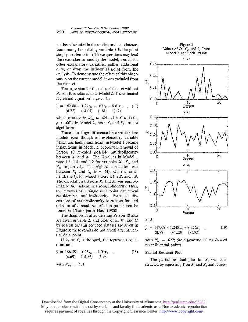
The diagnostics after deleting Person 10 alsoare given in Table 2, and plots of hi, Wi, and Cmby person for this reduced dataset are given inFigure 3; these results do not reveal any influen-tial data point.

If X, or X3 is dropped, the regression equa-tions are

with R;dj = .631

Figure 3Values of Ð¡, C¡, and h; FromModel 2 For Each Person

and

with R a 2&dquo;j = .627; the diagnostic values showedno influential points.

rtial Residual Plot

The partial residual plot for ~3 was con-structed by regressing Yon Xl and X2and retriev-



221

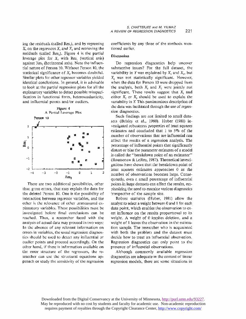
ing the residuals (called IZes,), and by regressingX~ on the regressors Xl and X2 and retrieving theresiduals (called Res2). Figure 4 is the partialleverage plot for X3 with IZes, (vertical axis)against Res, (horizontal axis). Note the influen-tial nature of Person 10. Without Person 10, thestatistical significance of X3 becomes doubtful.Similar plots for other regressor variables yieldedidentical conclusions. In general, it is advisableto look at the partial regression plots for all theexplanatory variables to detect possible misspeci-fication in functional form, heteroscedasticity,and influential points and/or outliers.

Figure 4A Partial Leverage Plot

~ .- A&dquo;’&dquo;

There are two additional possibilities, otherthan gross errors, that may explain the data forthe deleted Person 10. One is the possibility ofinteraction between regressor variables, and theother is the relevance of other unmeasured ex-

planatory variables. These possibilities must beinvestigated before final conclusions can bereached. Thus, a researcher faced with the

analysis of actual data may proceed in two ways:In the absence of any relevant information onerrors in variables, the usual regression diagnos-tics should be used to detect any influential oroutlier points and proceed accordingly. On theother hand, if there is information available onthe error structure of the regressors, the re-

searcher can use the structural equations ap-proach or study the sensitivity of the regression

coefficients by any three of the methods men-tioned earlier.

Discussion

Do regression diagnostics help uncover

substantive issues? For the full dataset, the

variability in Y was explained by X, and X,, butX2 was not statistically significant. However,when the data for Person 10 were dropped fromthe analysis, both X3 and X2 were jointly notsignificant. These results suggest that Xl andeither ~.’2 or X3 should be used to explain thevariability in Y This parsimonious description ofthe data was facilitated through the use of regres-sion diagnostics.

Such findings are not limited to small data-sets (Belsley et al., 1980). Huber (1981) in-

vestigated robustness properties of least squaresestimates and concluded that 1 to 5% of the

number of observations that are influential canaffect the results of a regression analysis. Thepercentage of influential points that significantlydistort or bias the parameter estimates of a modelis called the &dquo;breakdown point of an estimator&dquo;(Rousseeuw & LeRoy, 1987). Theoretical investi-gations have shown that the breakdown point ofleast squares estimates approaches 0 as thenumber of observations becomes large. Conse-quently, even a srnall percentage of influentialpoints in large datasets can affect the results, em-phasizing the need to examine various diagnosticsirrespective of the sample size.

Robust statistics (Huber, 1981) allow the

analyst to select a weight between 0 and 1 for eachdata point, which enables the observation to ex-ert influence on the results proportional to itsweight. A weight of 0 implies deletion, and aweight of 1 leaves the observation in the estima-tion sample. The researcher who is acquaintedwith both the problem and the dataset mustdecide how to treat an influential observation.

Regression diagnostics can only point to thepresence of influential observations.

Although commonly available regressiondiagnostics are adequate in the context of linearregression models, there are some situations in



222

which using regression diagnostics are inade-quate. The paper by Huber (1983) and the discus-sions following by several researchers and thesubsequent rejoinder by Huber provide a helpfulguide to the applied researcher. A study of theimpact of the usual regression diagnostics whenthe assumptions of the regression model areviolated (particularly the assumption of the in-dependence of errors) was studied by Polasek(1984). The behavioral researcher should be awareof situations in which the usual diagnostics maybe inadequate.

ultiple Influential Points

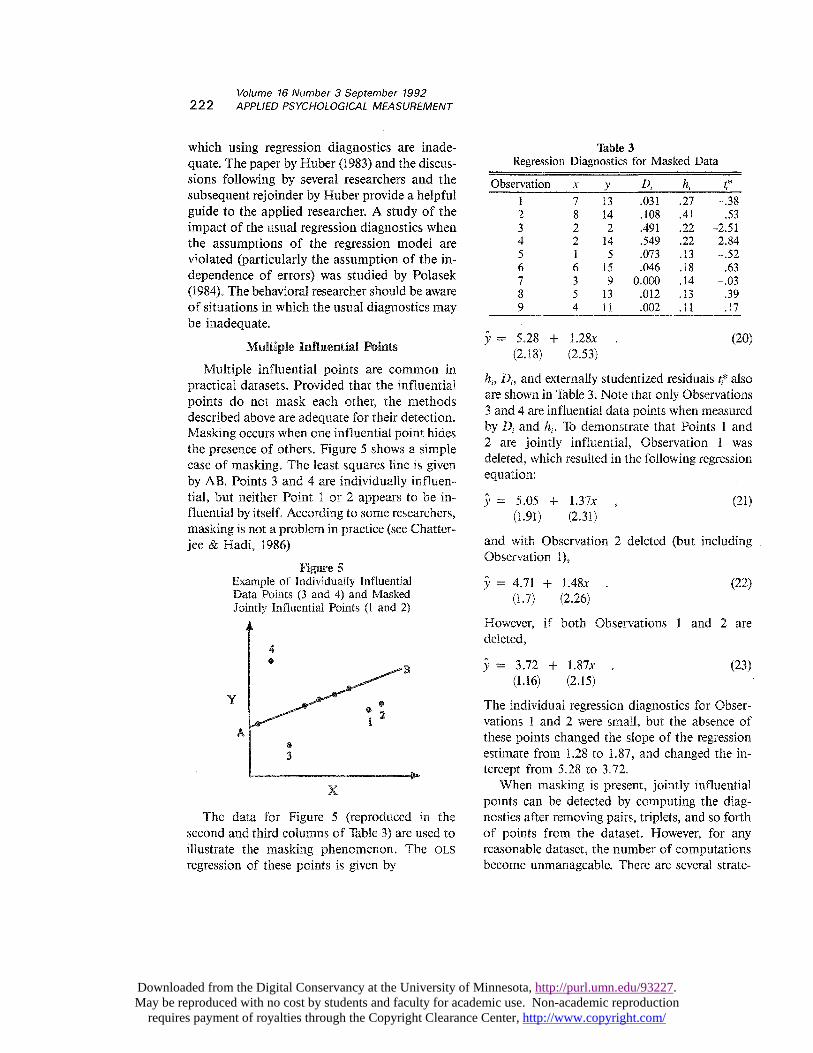
Multiple influential points are common inpractical datasets. Provided that the influentialpoints do not mask each other, the methodsdescribed above are adequate for their detection.Masking occurs when one influential point hidesthe presence of others. Figure 5 shows a simplecase of masking. The least squares line is givenby AB. Points 3 and 4 are individually influen-tial, but neither Point 1 or 2 appears to be in-fluential by itself. According to some researchers,masking is not a problem in practice (see Chatter-jee & Hadi, 1986).

Figure 5Example of Individually InfluentialData Points (3 and 4) and MaskedJointly Influential Points (1 and 2)

The data for Figure 5 (reproduced in thesecond and third columns of Table 3) are used toillustrate the masking phenomenon. The OLSregression of these points is given by

Table 3Regression Diagnostics for Masked Data

hi, 1~~, and externally studentized residuals t;* alsoare shown in Table 3. Note that only Observations3 and 4 are influential data points when measuredby D, and h,. To demonstrate that Points 1 and2 are jointly influential, Observation 1 was

deleted, which resulted in the following regressionequation:

and with Observation 2 deleted (but includingObservation 1),

However, if both Observations 1 and 2 are

deleted,

The individual regression diagnostics for Obser-vations 1 and 2 were small, but the absence ofthese points changed the slope of the regressionestimate from 1.28 to 1.87, and changed the in-tercept from 5.28 to 3.72.When masking is present, jointly influential

points can be detected by computing the diag-nostics after removing pairs, triplets, and so forthof points from the dataset. However, for anyreasonable dataset, the number of computationsbecome unmanageable. There are several strate-



223

gies to deal with this problem.The first approach uses the off-diagonal

elements of H. The off-diagonal elements of H,h,;, play a significant role in the determinationof joint influence. For example, a high value ofhij may indicate the presence of the joint in-fluence of the ith and the jth observations. Gray& Ling (1984) detected influential subsets inregression using a clustering algorithm. They pro-vided a graphical method for detecting jointly in-fluential points. For a more complete discussionof the use of off-diagonal elements of H fordetecting joint influence, see the discussion

following Gray & Ling (1984).The second strategy advocated by Rousseeuw

(1984) and Rousseeuw & Leroy (1987) uses theleast median squares (LMS) approach. With LMS,the estimates are obtained by minimizing themedian squared residuals and are robust in thepresence of multiple outlier points. The LMSestimates can be thought of as determining amedian or modal plane (model) and are notinfluenced by multiple outliers. Rousseeuw andLeroy discussed the properties of LMS estimatesand provided an algorithm for determining theLMS estimates and subsequent detection ofoutliers. Rousseeuw & Van Zomeren (1990) pro-vided an alternative approach, based on theMahalanobis distance, for unmasking multi-variate outliers and leverage points.A third strategy considers the data as n points

in a (k + 1)-dimensional space. The vertices ofthe convex hull (smallest convex set) of thesepoints are proposed as candidates for testing forjoint influence. Figure 6 presents the outermostconvex hull of a set of points in two-dimensionalspace. The vertices of the outermost layer (peel)are denoted by Points 1 through 8. This layer ofpoints may be removed in order to continue ex-amining vertices of inner hulls. This approach,which reduces the exhaustive search for multipleinfluential points, was proposed by Chatterjee &

Chatterjee (1990). It is still in an experimentalstage, as is the suggestion to examine each vertextogether with the points that are in the vicinityof that vertex. The convex hull approach was used

Figure 6The Outermost Convex Hull of a Set of Points

successfully by Chatterjee, Jamieson, & Wiseman

(1991) for detecting multiple influential points infactor analysis. Peeling of convex hulls for order-ing multivariate data can be found in Green (1984),and other uses of the vertices of convex hulls asextreme points are discussed in Barnett (1976).

Diagnostics for ultivariateRegression and Other Models

Multivariate Diagnostics

There appears to be very little work done onmultivariate diagnostics, other than the work ofHossain & Naik (1989). Residual-based, volume-based, and distance-based diagnostics for themultivariate regression model are discussed brief-ly. There appears to be no commonly availablesoftware to implement these, but the diagnosticsdescribed below can be computed using the PROCMATRIX command in SAS (SAS Institute, Inc.,1982).

Consider the multivariate regression model

where Y is a n x p response matrix of n obser-vations of p response variables,

X is a n x (k + 1) matrix of regressors,B is a (k + 1) x p matrix of parameter

values, andE is a n x p matrix of residuals.



224

The columns of B are denoted by b;. X isassumed to be nonstochastic and of full rank,[i.e., rank(X) = k + 1]. Rows ei of E are

assumed to be independent and normallydistributed, with a p x 1 mean vector of Os anda p x p covariance matrix ~. The least squaresestimates of bj are given by

which is the same as equation-by-equation leastsquares estimation.

First, note that the diagonal elements hi of H,the prediction matrix, play the same role as inmultiple regression. Large values indicate that atleast one component of the ith data point maybe an influential point.

The residual matrix is given by E = Y - X ~.An estimate of ~, is

Let

where f,~ = Y~t~ - X(i)B(i) is obtained by drop-ping the ith observation. Define

and

where ~2 and T? are the multivariate analogues ofti and t/ discussed earlier. These statistics are ap-proximately distributed as Hotelling’s T’2 dis-tribution and can be tested for an outlier by com-paring their values to the upper percentage pointof an F distribution with appropriate degrees offreedom.A multivariate analogue of Di is given by

Influence of the ith observation on the estimateof B is indicated by large values of 17*

Jlg can be modified accordingly as

where Fcx,p,n - k - p - is an upper percentage pointof the F distribution vaith p and z - p - 1)degrees of freedom.

C¡* is the corresponding multivariate analogueof the scalar variances and is given by

As before, very high or very low values of C* areconsidered to be significant. Hossain & Naik

(1989) discussed other multivariate diagnosticmeasures for regression.

Nonlinear Models

Many nonlinear models and generalized linearmodels -including logistic regression and sur-vival models -(McCullagh & Nelder, 1984) havebecome popular in the social sciences due to theenhanced capability they offer in building ex-planatory models. Nonlinear regression param-eters can be very sensitive to values that are ex-

treme in the response space or in the explanatoryvariables. One particular difficulty with nonlinearregression is that the diagnostics cannot be ob-tained in closed analytic form as in linear regres-sion, and specific diagnostic routines must bebuilt into each nonlinear regression program.Diagnostics for logistic regression and their ap-plications to other nonlinear models have been



225

described by Pregibon (1981) and Jorgenson(1983). Unfortunately, no suitable computerpackage exists that computes and provides non-linear regression diagnostics on a routine basis.

Other ultivariat~ Methods

Influential data points also can exert con-siderable influence on the results of principalcomponents and factor analysis models. Theestimates of eigenvalues, eigenvectors, factor

loadings, and factor scores can be altered

dramatically by the presence of a small set ofinfluential observations. A statistic similar to

A, was proposed by Chatterjee et al. (1991)that detects influential observations in principalcomponents and factor analysis models. Com-putational requirements also are discussed

by these authors, but commercial computerpackages for detecting influential data pointsin principal and factor analysis models are notyet available.

Summary and Conclusions

Regression models need to be examined

beyond the usual summary statistics and tests ofsignificance. This is especially important whenbehavioral variables are involved, because of theinherent difficulties and errors in the measure-ment of these variables. Five regressiondiagnostics were recommended for a sound

analysis of data: (1) hi, the diagonal elements ofthe prediction matrix; (2) t;f the externallystudentized residual; (3) 1~;, Cook’s distance; (4)the Welsch-Kuh distance; and (5) C&dquo; thecovariance ratio. These numeric measures shouldbe supplemented with graphical tools, such as avariety of residual plots.

Use of regression diagnostics often reveals datapoints whose presence will affect the estimatesand significance of the parameters. As low as 1%of influential data points may render one or morevariables significant or insignificant, may induceor remove multicolinearity, and may changeestimates of parameter vectors and other statisticsin an unpredictable way.

Applications of regression diagnostics in other

multivariate models such as cluster analysis, andcausal models such as path analysis and LISRELmodels, have not yet appeared in the literature.Developments of both theory and computerpackages to detect outliers in nonlinear regres-sion, weighted least squares, two-stage least

squares, and other multivariate models also

should be useful.The interplay between measurement error,

regression diagnostics, and cross-validation is aninteresting one. Very little work has been doneon the relationship between cross-validation andregression diagnostics and how to combine theprocedures for useful data analysis. The relation-ship between measurement errors and regressiondiagnostics is easier to comprehend. Measure-ment errors, if arising due to an underlying causalmechanism, obviously can be modeled. However,when the underlying causal mechanisms givingrise to the measurement errors are unknown ordifficult to model, then the measurement errorswill be confounded with influential points andoutliers. In that case, treatment of data by regres-sion diagnostics will not address the problemsarising from measurement errors.

Wellman & Gunst (1991) studied how influen-tial observations affect linear measurement esti-mators. Their results indicate that the effects ofinfluential observations are in a direction or-

thogonal to and along the fitted plane, ratherthan vertically and horizontally. They developeddiagnostics patterned after least squares diagnos-tics, but these diagnostics follow the methodsused for developing diagnostics for nonlinearregression and generalized linear models.

The techniques of regression diagnostics candetect influential points and what would happenif such points are removed from the analysis, butthey do not answer many important questions.In particular, whether to keep or remove suchdata points cannot be answered in an abstract set-ting. Very often, bringing attention to a small setof unusual data points is a first step that canultimately reveal much about the process understudy. If the purpose of most data analysis ismodel building, regression diagnostics and



226

various versions of cross-validation can be seenas different activities with a common purpose.Efron (1979) suggested that further research maylead to powerful combinations of cross-

validation, the jackknife, and the bootstrap.

References

Atkinson, A. C. (1985). Plots, transformations, andregression. Oxford, England: Oxford UniversityPress

Barnett, V. (1976). Ordering multivariate data (withdiscussion). Journal of the Royal Statistical Society,139, (Series A), 318-354.

Belsley, D. A. (1984). Demeaning condition diagnosticsthrough centering (with discussion). The AmericanStatistician, 38, 73-93.

Belsley, D. A., Kuh, E., & Welsch, R. E. (1980). Regres-sion diagnostics: Identifying influential data andsources of collinearity. New York: Wiley.

Bollen, K. A. (1989). Structural equations with latentvariables. New York: Wiley.

Bollen, K. A., & Jackman, R. W. (1985). Regressiondiagnostics: An expository treatment of outliers andinfluential cases. Sociological Methods and Research,13, 510-542.

Box, G. E. P. (1983). Apology for equimenicism instatistics. In G. E. P. Box & C. F. Wu (Eds.), Scien-tific inference and data analysis (pp. 121-145). NewYork: Wiley.

Casella, G. (1983). Leverage and regression through theorigin. The American Statistician, 37, 147-151.

Chatterjee, S., & Chatterjee, S. (1990). Convex hull ofa set of points. Computational Statistics and DataAnalysis, 10, 87-92.

Chatterjee, S., & Hadi, A. S. (1986). Influential obser-vations, high leverage points and outliers in linearregression (with discussion). Statistical Science, 1,379-415.

Chatterjee, S., & Hadi, A. S.(1988). Sensitivity in linearregression. New York: Wiley.

Chatterjee, S., Jamieson, L., & Wiseman, F. (1991).Diagnostics in factor analysis. Marketing Science,10, 145-160.

Chatterjee, S., & Price, B. P. (1973). Regression analysisby example. New York: Wiley.

Chatterjee, S., & Wiseman, F. (1984). Use of regres-sion diagnostics in political science research.American Journal of Political Science, 27, 601-613.

Chesher, A. (1991). The effect of measurement error.Biometrika, 78, 451-462.

Cochran, W. G. (1972). Some effects of errors ofmeasurement on linear regression. In J. Neyman(Ed.), Proceedings of the 6th Berkeley Symposium,

1, 527-539.Cook, R. D. (1986). Assessment of local influence (with

discussion). Journal of the Royal Statistical Society,46, (Series B), 133-169.

Cook, R. D., & Weisberg, S. (1980). Characterizationof an empirical influence function for detecting in-fluential cases in regression. Technometrics, 22,495-508.

Cook, R. D., & Weisberg, S. (1982a). Residuals and in-fluence in regression. New York: Chapman and Hall.

Cook, R. D., & Weisberg, S. (1982b). Criticism andinfluence analysis in regression. In S. Leinhardt

(Ed.), Sociological Methodology (pp. 313-361).Daniel, C., & Wood, F. S. (1980). Fitting equations to

data: Computer analysis of multifactor data (2nd ed.).New York: Wiley.

Darlington, R. B. (1990). Regression and linear models.New York: McGraw Hill.

Delaney, N. J., & Chatterjee, S. (1986). Use of thebootstrap and cross-validation in ridge regression.Journal of Business and Economics Statistics, 4,255-261.

Dixon, W. J. (Ed.). (1984). BMDP statistical software.Berkeley CA: University of California Press.

Fuller, W. A. (1987). Measurement error models. NewYork: Wiley.

Gray, J. B., & Ling, R. F. (1984). K-Clustering as adetection for influential subsets in regression (withdiscussion). Technometrics, 26, 305-330.

Green, P. J. (1984). Peeling of bivariate data. In V.Barnett (Ed.), Interpreting multivariate data (pp.235-271). New York: Wiley.

Heller, G. (1987). Fixed sample results for linear modelswith measurement error. Unpublished doctoral

dissertation, New York University.Hossain, A., & Naik, D. N. (1989). Detection of in-

fluential observations in multivariate regression.Journal of Applied Statistics, 16, 21-32.

Huber, P. (1981). Robust statistics. New York: Wiley.Huber, P. J. (1983). Minimax aspects of bounded-

influence regression (with comments). Journal of theAmerican Statistical Association, 78, 66-80.

Jorgenson, B. (1983). Maximum likelihood estimationand large sample inference by generalized linear andnonlinear regression models. Biometrika, 70, 19-28.

Judge, G. G., Griffith, W. L., Hill, R. C., & Lee, T.C. (1980). The theory and practice of econometrics.New York: Wiley.

Lord, F. M., & Novick, M. R. (1968). Statistical theoriesof mental test scores. Reading MA: Addison-Wesley.

Malinvaud, E. (1970). Statistical methods in

econometrics. Amsterdam: North Holland.Mansfield, E. R., & Helms, B. P. (1982). Detecting

multicollinearity. The American Statistician, 36,158-160.



227

McCullagh, P., & Nelder, J. A. (1984). Generalizedlinear models. New York: Chapman and Hall.

Mosteller, F., & Tukey, J. W. (1977). Data analysis andregression. Reading MA: Addison-Wesley.

Nunnally, J. C. (1967). Psychometric theory. New York:McGraw Hill.

Pedhazur, E. (1982). Multiple regression in behavioralresearch. New York: Holt, Rinehart & Winston.

Picard, R. R., & Berk, K. N. (1990). Data splitting.The American Statistician, 44, 140-147.

Picard, R. R., & Cook, R. D. (1984). Cross-validationof regression models. Journal of the AmericanStatistical Association, 79, 575-583.

Pregibon, D. (1981). Logistic regression diagnostics. TheAnnals of Statistics, 9, 705-724.

Polasek, W. (1984). Regression diagnostics for generallinear regression models. Journal of the AmericanStatistical Association, 79, 79-86.

Rousseeuw, P. J. (1984). Least median squares of

regression. Journal of the American Statistical

Association, 79, 871-880.Rousseeuw, P. J., & LeRoy, A. N. (1987). Robust regres-

sion and outlier detection. New York: Wiley.Rousseeuw, P. J., & van Zomeren, B. C. (1990). Un-

masking multivariate outliers and leverage points.Journal of the American Statistical Association, 85,633-639.

Ryan, B. F., Joiner, B. L., & Ryan, T. A. (1991).MINITAB handbook (2nd ed.). Boston MA: DuxburyPress.

SAS Institute, Inc. (1982). SAS user’s guide: Basics.Cary NC: Author.

SPSS, Inc. (1988). SPSS-X user’s guide (3rd ed.).

Chicago IL: Author.Stefanski, L. A. (1985). The effect of measurement

error on parameter estimation. Biometrika, 72,583-592.

Stevens, J. P. (1984). Outliers and influential data

points in regression analysis. Psychological Bulletin,95, 334-344.

Stewart, G. W. (1987). Collinearity and least squaresregression. Statistical Science, 2, 68-100.

Velleman, P. F., & Welsch, R. E. (1981). Efficient com-puting of regression diagnostics. American Statisti-cian, 35, 234-242.

Wellman, J. M., & Gunst, R. F. (1991). Influence

diagnostics for linear measurement error models.Biometrika, 78, 373-380.

Welsch, R. E., & Kuh, E. (1977). Linear regressiondiagnostics (Tech. Rep. No. 923-77). Cambridge:Massachusetts Institute of Technology, SloanSchool of Management.

Wilkinson, L. (1992). SYSTAT: Statistics (Version 5.2).Evanston IL: SYSTAT, Inc.

Acknowledgments

Tlae authors appreciate the advice of two anonymousreferees, which considerably improved the paper.

Author’s Address

Send requests for reprints or further information toSangit Chatterjee, Northeastern University, 219 HaydenHall, 360 Huntington Avenue, Boston MA 02115,U.S.A.



Date post:	11-Feb-2022
Category:	Documents
Upload:	others
View:	1 times
Download:	0 times

A Review of Regression Diagnostics - Conservancy - University of

Documents