1 A Rough Guide to RASP 2.1 (Beta) (Former S-DIVA ) 19/11/2012 Yan Yu 1 , AJ Harris 2 and Xingjin He 1 1 Key Laboratory of Bio-Resources and Eco-Environment of Ministry of Education, College of Life Sciences, Sichuan University, Chengdu, Sichuan, 610065, P. R. China. Email: [email protected]2 Department of Botany, Oklahoma State University, 104 Life Sciences East, Stillwater, Oklahoma 74078-3013 USA. Email: [email protected]
Transcript
1
A Rough Guide to RASP 2.1 (Beta)
(Former S-DIVA )
19/11/2012
Yan Yu 1, AJ Harris 2 and Xingjin He1
1 Key Laboratory of Bio-Resources and Eco-Environment of Ministry of Education, College of Life Sciences,
Sichuan University, Chengdu, Sichuan, 610065, P. R. China. Email: [email protected]
2 Department of Botany, Oklahoma State University, 104 Life Sciences East, Stillwater, Oklahoma
Contents A Rough Guide to RASP ................................................................................................................................................. 1
3. A simple RASP tour step by step ................................................................................................................................. 6
4. How to ....................................................................................................................................................................... 18
4.1 How to make a Trees data set. ............................................................................................................................ 18
4.2 How to make a Final tree. .................................................................................................................................... 19
4.3 How to make a Distributions file .......................................................................................................................... 20
We have written RASP (Reconstruct Ancestral State in Phylogenies) software to implements Bayesian Binary MCMC
(BBM), time-events curve analysis and Dispersal-Vicariance Analysis (S-DIVA) methods. RASP is easy-to-install on the
Windows, Mac, and Linux platforms, provides a user-friendly graphical interface, and generates exportable graphical results.
The BBM and time-events curve algorithms have been described in Yu et al. (2011, submitted). If you are using the
S-DIVA method, you may also want to cite Yu et al. (2010).
In RASP, the module of S-DIVA analysis is modified from source code of DIVA 1.2 (Ronquist, 2001) and the MCMC
analysis in BBM is modified from source code of Mrbayes 3.1.2 (Ronquist and Huelsenbeck, 2003). DEC models of
geographic range evolution was described in Ree et al. (2005) and Ree and Smith (2008). DEC analysis is modified from
source code of c++ version of Lagrange developed by Smith (2010).
1.2 Citation
A manuscript describing the RASP program has been submitted. Please cite the manuscript after it has been
published. In the meantime, please cite the program and our pervious paper (see below).
Program:
Yu Y., Harris A.J., He X.J. 2012. RASP (Reconstruct Ancestral State in Phylogenies) 2.1b. Available at
http://mnh.scu.edu.cn/soft/blog/RASP
S-DIVA method:
Yu Y, Harris AJ, He XJ. 2010. S-DIVA (statistical dispersal-vicariance analysis): a tool for inferring biogeographic
histories. Molecular Phylogenetics and Evolution , 56(2):848-850
DEC model:
Ree, R H and S A Smith. 2008. Maximum likelihood inference of geographic range evolution by dispersal, local extinction,
and cladogenesis. Systematic Biology 57(1): 4-14.
Ree, R H, B R Moore, C O Webb, and M J Donoghue. 2005. A likelihood framework for inferring the evolution of
geographic range on phylogenetic trees. Evolution 59(11): 2299-2311
4
User's Guide:
Yu Y, AJ Harris, and X He. (2012). A rough guide to RASP. Available online at http://mnh.scu.edu.cn/soft/blog/RASP.
5
2. Installing (back to contents)
For windows users: Supported Operating Systems: Windows NT, 2000, 2003, 2008, XP, Vista and Windows 7 System Requirement:
If you are using Windows 2000, 2003 or XP, please make sure that Microsoft® .NET 2 Framework is installed on your computer. This is usually installed through Windows updates but may be absent from older systems. The .NET framework 2 packages are available for free here and should be installed prior to using RASP.
For Mac users: Supported Operating Systems: 10.4.x, 10.5.x, 10.6.x System Requirement:
This version of RASP is developed for use on Mac OS X versions 10.5 and above on computers with Intel processors only. RASP for Mac uses the Wine program in order for RASP to run. Wine is installed automatically when you run the application for the first time.
For Linux users: Supported Operating Systems: All Linux distribution System Requirement:
You need Mono runtime and Mono-vbnc to run RASP. Mono is a software platform designed to allow developers to easily create cross platform applications. The Mono Framework packages are available for free here.
IMPORTANT: For Ubuntu 10.x and Debian 6.x users: Mono runtime comes pre-installed with Ubuntu. You may simply use “sudo apt-get install mono-vbnc” to install Mono-vbnc. For Debian 6.x users: Please use "Root Terminal" to run RASP and RASP must be loaded in its own folder. For instance: 1.Change the dictionary to RASP's folder: 'cd /home/user/Desktop/RASP' 2. Run RASP: 'sh ./RASP-Linux'
IMPORTANT NOTE FOR ALL PLATFORMS:
Please make sure that the decimal symbol of your system is ‘.’
6
3. A tour of RASP step by step (back to contents)
3.1 Preparation
You need: 1. Trees data set and/or a ‘final tree’
(A sample trees data file: “sample\sample1.tree”) -[How to]: How to obtain trees data set from BEAST (Drummond and Rambaut, 2006)
-[How to]: How to obtain trees data set from PAUP (Swofford, 2003) -[How to]: How to obtain trees data set from other phylogenetic programs.
(A sample final tree: “sample\Sample1_Final_Tree.tre”) -[How to]: How to make a final tree using BEAST.
-[How to]: How to make a final tree using PAUP. -[How to]: How to obtain a final tree from other phylogenetic programs.
2. Distributions file (not required). (A sample distributions file: “sample\Sample1_Distribution.csv”) -[How to]: How to input distributions in RASP.
-[How to]: How to make a Distributions file. Launch RASP
1. Open [File > Load Trees] and navigate to your trees data set and select it. [Example: Open “Sample1.trees” in folder Sample]
Note1: In Bayesian Binary MCMC (BBM) analysis, only one final tree is needed Note2: If you only have one tree, you could load it with [File > Load Single Tree] and jump to step 3.
Note3: For a large dataset, one can try [File > Quick Load Trees] to be faster, but only trees exported from Beast and mrbayes were supported
2. Have a ‘final tree’: open [File>Condense tree>Load Exiting Tree], navigate to your final tree file and select it.
Do not have a ‘final tree’: use [File>Condense tree>Compute condense] to build one. [Example: Open “Sample1_Final_Tree.tre” in folder Sample] Note1: The condensed (consensus) tree will be a majority rule consensus with compatible groups with less than 50% support allowed. The tree consensus is computed using Consense (Felsenstein, 1993) from your trees file or from the subset of trees from the file you have specified (i.e., see the Random Trees, and Discard Trees options below).
3. If you have a distributions file:Open [File > Load Distribution],navigate to your file and select it. You can also input and revise the distributions in the entry fields in the Distribution column in RASP.
[Example: Open “Sample1_Distribution.csv” in folder Sample]
7
3.2 Options
Note: “(S)” means this option applies to Statistical Dispersal-Vicariance Analysis, “(B)” means this option applies to Bayesian Binary MCMC Analysis.
Binary trees (S): The total number of binary trees in your trees data set. Amount of trees (B): The total number of trees in your trees data set. Note: The Statistical Dispersal-Vicariance Analysis requires binary trees while Bayesian Binary MCMC Method accepts one polytomies tree. Discard trees (S): The number of trees that will be discarded from the beginning of the trees data set; equivalent to a burnin. Random tree (S): Select random trees form trees data set to run the analysis. Trees will be selected from between Discard Trees and Amount of trees. You can save the randomly selected trees to a new file with [File> Save Processed Trees]. Use Tree File: Run Statistical Dispersal-Vicariance Analysis or Bayesian binary MCMC Analysis for all nodes in the final tree. Use ancestral ranges of this tree (S): The final tree will be optimized. Only ancestral ranges with F>0 for a node in the final tree will be considered in the calculation of F using all trees for the node. For example: There are 3 trees in the trees data set. In each tree, there is a node y. The following are the DIVA results of the node y of the 3 trees and the final tree:
tree1: A, AB, C tree2: A, B, AB tree3: A, B, AB final tree: A, B
In this case, if "Use Ancestral Ranges of this Tree" is unselected, the S-DIVA result of node y is: 3/9A, 2/9B, 1/9C and 3/9AB. If "Use Ancestral Ranges of this Tree" is selected, the S-DIVA result of node y is: 3/5A and 2/5B. The ranges C and AB were discarded, because they do not exist in the result of the final tree. (A sample DIVA output file: Sample\Sample1_DIVA_output.txt). Estimate a particular node: Run RASP only for specified nodes. Check this to allow the following three options. You can specify a node using the following format: 1,2,3,4,5 or 1-5 1,2,3,4,8,9,10 or 1-4,8-10 (Numbers correspond to IDs in the Distributions column in the RASP interface.) Note: If using RASP to estimate a particular node, you do not need a final tree. However, if you load a final tree, you will be able to select the node you want to perform an analysis for by using the drop down menu to the right of the node entry field. With an undefined sister (x) (S): Estimate the ancestral range of the clade and an undefined sister (x) (Harris & Xiang, 2009). Specify the node using one of the formats shown above. Note: The result will be for the stem (parent node) of the clade or node you specify. With omitted taxon distributed in (S): Add distribution information for a taxon omitted from the phylogeny. RASP manually places the unnamed taxon as sister to node specified using Estimate P for a single node and considers its distribution when running the analysis. Notes: The manually placed taxon is not included in graphical output. The option to include the relationship and distribution of an omitted taxon is only available when using the Estimate P for a single node option. Node List (B): In Bayesian Binary MCMC Analysis, you can deselect nodes to exclude them from the analysis. Using the Select > n% options, you can select all nodes supported by posterior probability (pp) greater than your specified value. Note: In order to select nodes with greater than n% pp support,
8
3.3 Analysis
3.3.1. Statistical Dispersal-Vicariance Analysis Choose [Analysis > Statistical Dispersal Vicariance Analysis] to use default options to run Analysis.
[Options] Allow Reconstruction: Unchecking this option changes the method used for calculating F(xn) from i/Dt to 1/N. See section 3.4.1 below. Also see Yu et al. (2010) and Harris & Xiang (2009) in which the differences between these options are discussed. Max areas: The number of unit areas allowed in ancestral distributions. Bound and Hold: These two options are the same as in DIVA 1.2. Default settings in S-DIVA are the maximum values. Note: If you need additional help with the [Optimize] options Bound and Hold, or with
setting the command line, we recommend reviewing these options in DIVA 1.2 (command: help;) and the DIVA 1.1 User's Manual (Ronquist, 1996). Set command for final tree: Set the optimize command for the final tree separately. Selecting this option means that range frequencies and probabilities will be calculated for the final tree only. For example: There are 3 trees in the trees data set. In each tree, there is a node y. The following are the DIVA results of the node y of the 3 trees and the final tree:
tree1: A, AB, C tree2: A, B, AB tree3: A, B, AB final tree: A, B
If you only use the result for the final tree, the result is: 1/2A and 1/2B. For most S-DIVA analyses, you will want this box unchecked. If using this option, note that S-DIVA cannot handle the reset command in DIVA or any of its options. Include -> and Exclude-<: Include or exclude ranges from calculation. This can be accomplished by selecting ranges from the Include list and clicking the arrow to move them to exclude. When you do this, only the selected ranges will be excluded. You can also exclude all ranges that include a particular subset of areas using the range matrix. For example, unchecking the box in the first row, second column will remove all ranges that include A and B; AB and ABC in the example above. Once the desired boxes have been unchecked, [Operation> Refresh the Range List]. Note: Excluded ranges are still considered by DIVA. However, they are removed from frequency calculations performed by S-DIVA. Allow excluded areas when null: S-DIVA returns a null result if all optimal ranges for a node have been excluded from the analysis. This is because DIVA cannot seek suboptimal range solutions. 3.3.2. Bayesian Binary Method (BBM) Choose [Analysis > Bayesian Binary Method] to use default options to run Analysis.
9
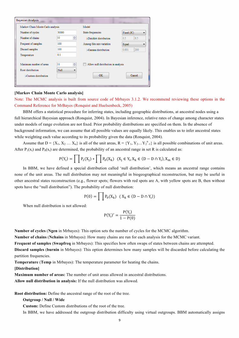
[Markov Chain Monte Carlo analysis] Note: The MCMC analysis is built from source code of Mrbayes 3.1.2. We recommend reviewing these options in the Command Reference for MrBayes (Ronquist and Huelsenbeck, 2005)
BBM offers a statistical procedure for inferring states, including geographic distributions, at ancestral nodes using a full hierarchical Bayesian approach (Ronquist, 2004). In Bayesian inference, relative rates of change among character states under models of range evolution are not fixed. Prior probability distributions are specified on them. In the absence of background information, we can assume that all possible values are equally likely. This enables us to infer ancestral states while weighting each value according to its probability given the data (Ronquist, 2004).
Assume that D = {X1, X2 … Xn} is all of the unit areas, R = {Y1, Y2…Y2n
-1} is all possible combinations of unit areas. After P1(xi) and P0(xi) are determined, the probability of an ancestral range in set R is calculated as:
P Y! = P!(X!) ∗ P!(X!) (X! ∈ Y!, X! ∈ D − D ∩ Y! , X! ∈ D)
In BBM, we have defined a special distribution called ‘null distribution’, which means an ancestral range contains none of the unit areas. The null distribution may not meaningful in biogeographical reconstruction, but may be useful in other ancestral states reconstruction (e.g., flower spots; flowers with red spots are A, with yellow spots are B, then without spots have the “null distribution”). The probability of null distribution:
P 0 = P!(X!) ( X! ∈ D − D ∩ Y! )
When null distribution is not allowed:
P Y! ′ =P Y!
1 − P(0)
Number of cycles (Ngen in Mrbayes): This option sets the number of cycles for the MCMC algorithm. Number of chains (Nchains in Mrbayes): How many chains are run for each analysis for the MCMC variant. Frequent of samples (Swapfreq in Mrbayes): This specifies how often swaps of states between chains are attempted. Discard samples (burnin in Mrbayes): This option determines how many samples will be discarded before calculating the partition frequencies. Temperature (Temp in Mrbayes): The temperature parameter for heating the chains. [Distribution] Maximum number of areas: The number of unit areas allowed in ancestral distributions. Allow null distribution in analysis: If the null distribution was allowed. Root distribution: Define the ancestral range of the root of the tree. Outgroup / Null / Wide
Custom: Define Custom distributions of the root of the tree. In BBM, we have addressed the outgroup distribution difficulty using virtual outgroups. BBM automatically assigns
10
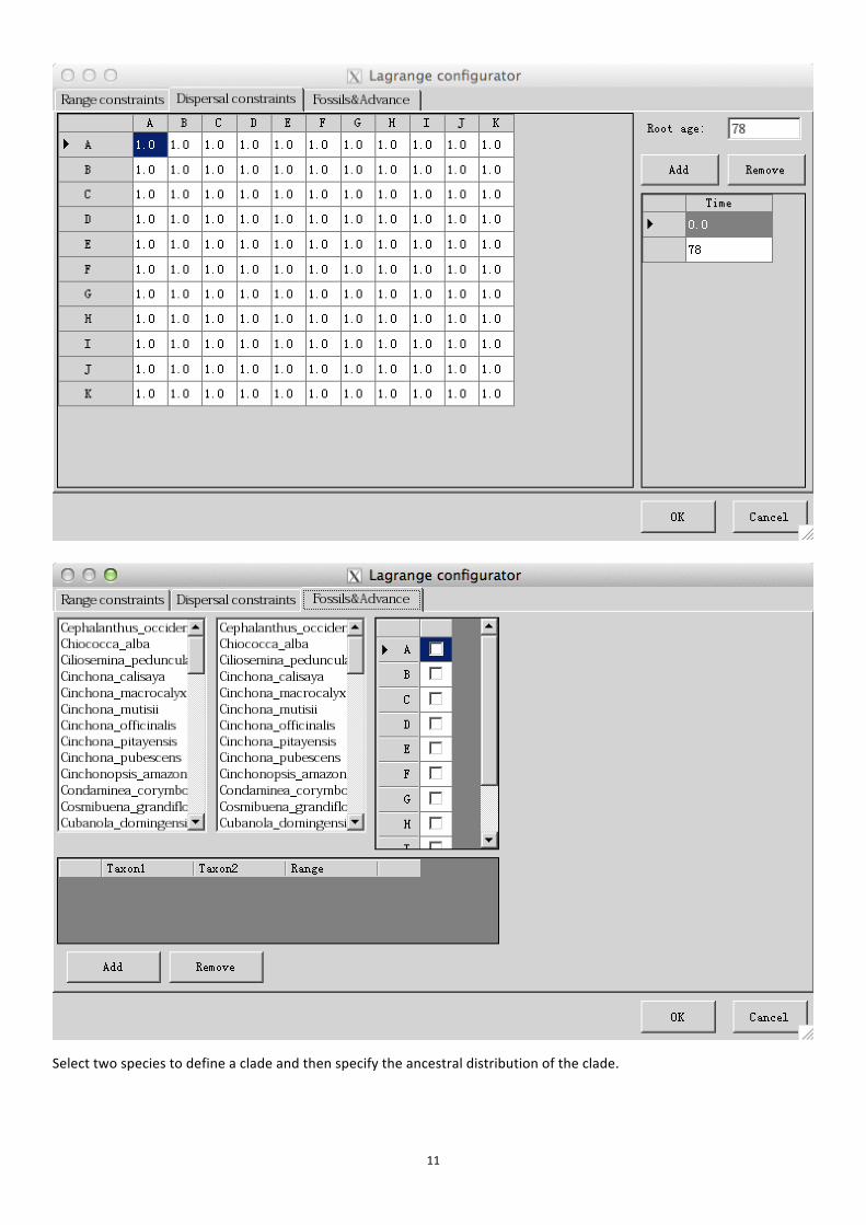
two virtual outgroups to the original phylogenetic tree prior to the start of an analysis. When the real distribution or ancestral distribution of the outgroups are known, the virtual outgroups may be coded according to the real distributions ("custom" in RASP). When the outgroup distributions are unknown, or considered too wide, too derived, or too distant to be useful, the ranges of the virtual groups may be coded as "wide" or "null". Under the wide distribution, the virtual outgroups are coded to occur in all areas occupied by the ingroup. Under the null distribution, the outgroup is assigned to a new area in which none of the ingroup OTUs occur. We recommend comparing results from custom, wide, and null settings when performing historical biogeographic reconstructions using BBM. IMPORTANT: This option has great influence on the result. If you do not know which root distribution to use, you may need to try each of them to determine their effects on your results. [Model] Note: There are four models in Bayesian Binary MCMC Analysis: JC, JC+G, F81, F81+G State frequencies: Character state frequencies. Among-site rate variation: This parameter specifies the prior for the gamma shape parameter for among-site rate variation. 3.3.3. Dispersal-Extinction-Cladogenesis (DEC) Model Choose [Analysis > Dispersal-Extinction-Cladogenesis Model] to use DEC models of geographic range evolution described in Ree et al. (2005) and Ree and Smith (2008). This module use source code of c++ version of Lagrange developed by Smith (2010) and is much more faster than the Python version of Lagrange.
Include -> and Exclude-<: Include or exclude ranges from calculation. This can be accomplished by selecting ranges from the Include list and clicking the arrow to move them to exclude. When you do this, only the selected ranges will be excluded. You can also exclude all ranges that include a particular subset of areas using the range matrix. For example, unchecking the box in the first row, second column will remove all ranges that include A and B; AB and ABC in the example above. Maximum areas at each node: The number of unit areas allowed in ancestral distributions. Automatic add possible ranges: If there are too few ranges to do the analysis, RASP will add possible ranges automaticity.
11
Select two species to define a clade and then specify the ancestral distribution of the clade.
12
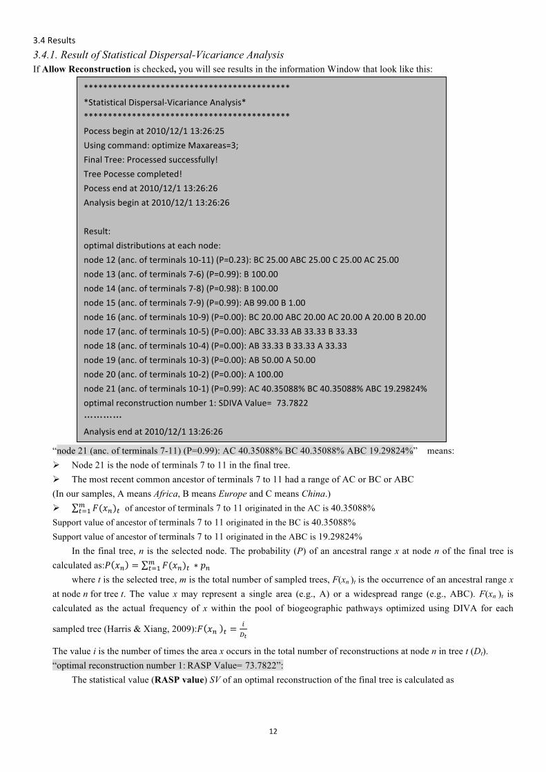
3.4 Results 3.4.1. Result of Statistical Dispersal-Vicariance Analysis If Allow Reconstruction is checked, you will see results in the information Window that look like this:
“node 21 (anc. of terminals 7-11) (P=0.99): AC 40.35088% BC 40.35088% ABC 19.29824%” means: Ø Node 21 is the node of terminals 7 to 11 in the final tree. Ø The most recent common ancestor of terminals 7 to 11 had a range of AC or BC or ABC (In our samples, A means Africa, B means Europe and C means China.) Ø 𝐹(𝑥!)!!
!!! of ancestor of terminals 7 to 11 originated in the AC is 40.35088% Support value of ancestor of terminals 7 to 11 originated in the BC is 40.35088% Support value of ancestor of terminals 7 to 11 originated in the ABC is 19.29824%
In the final tree, n is the selected node. The probability (P) of an ancestral range x at node n of the final tree is calculated as:𝑃 𝑥! = 𝐹(𝑥!)! !
!!! ∗ 𝑝! where t is the selected tree, m is the total number of sampled trees, F(xn )t is the occurrence of an ancestral range x
at node n for tree t. The value x may represent a single area (e.g., A) or a widespread range (e.g., ABC). F(xn )t is calculated as the actual frequency of x within the pool of biogeographic pathways optimized using DIVA for each
sampled tree (Harris & Xiang, 2009):𝐹 𝑥! ! =!!!
The value i is the number of times the area x occurs in the total number of reconstructions at node n in tree t (Dt). “optimal reconstruction number 1: RASP Value= 73.7822”:
The statistical value (RASP value) SV of an optimal reconstruction of the final tree is calculated as
******************************************* *Statistical Dispersal-‐Vicariance Analysis* ******************************************* Pocess begin at 2010/12/1 13:26:25 Using command: optimize Maxareas=3; Final Tree: Processed successfully! Tree Pocesse completed! Pocess end at 2010/12/1 13:26:26 Analysis begin at 2010/12/1 13:26:26 Result: optimal distributions at each node: node 12 (anc. of terminals 10-‐11) (P=0.23): BC 25.00 ABC 25.00 C 25.00 AC 25.00 node 13 (anc. of terminals 7-‐6) (P=0.99): B 100.00 node 14 (anc. of terminals 7-‐8) (P=0.98): B 100.00 node 15 (anc. of terminals 7-‐9) (P=0.99): AB 99.00 B 1.00 node 16 (anc. of terminals 10-‐9) (P=0.00): BC 20.00 ABC 20.00 AC 20.00 A 20.00 B 20.00 node 17 (anc. of terminals 10-‐5) (P=0.00): ABC 33.33 AB 33.33 B 33.33 node 18 (anc. of terminals 10-‐4) (P=0.00): AB 33.33 B 33.33 A 33.33 node 19 (anc. of terminals 10-‐3) (P=0.00): AB 50.00 A 50.00 node 20 (anc. of terminals 10-‐2) (P=0.00): A 100.00 node 21 (anc. of terminals 10-‐1) (P=0.99): AC 40.35088% BC 40.35088% ABC 19.29824% optimal reconstruction number 1: SDIVA Value= 73.7822 ………… Analysis end at 2010/12/1 13:26:26
13
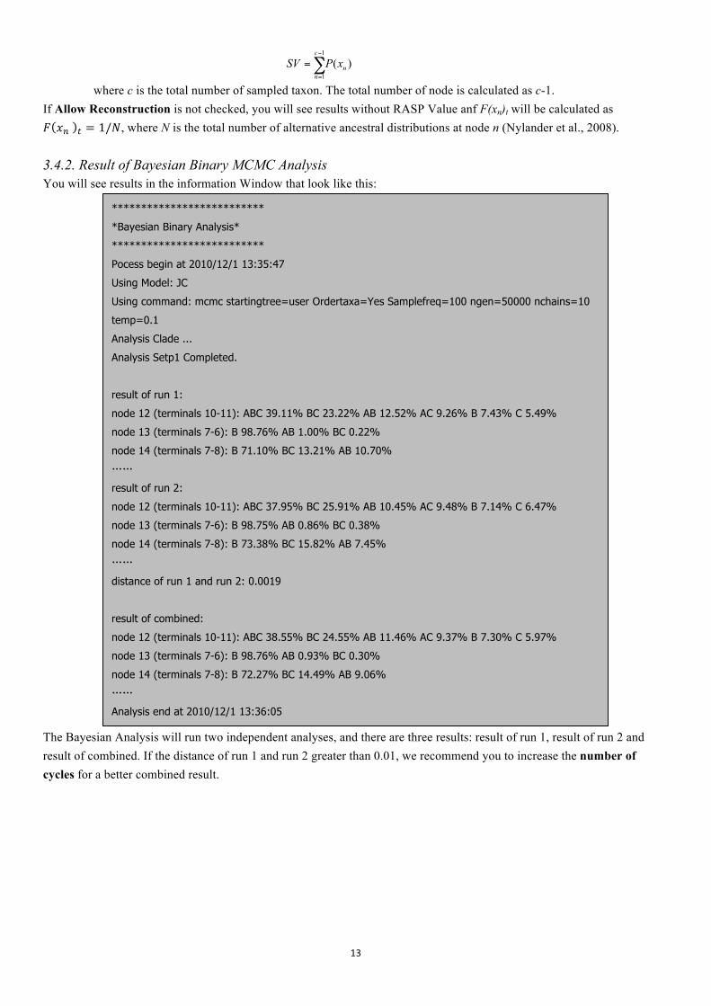
where c is the total number of sampled taxon. The total number of node is calculated as c-1. If Allow Reconstruction is not checked, you will see results without RASP Value anf F(xn)t will be calculated as 𝐹 𝑥! ! = 1/𝑁, where N is the total number of alternative ancestral distributions at node n (Nylander et al., 2008). 3.4.2. Result of Bayesian Binary MCMC Analysis You will see results in the information Window that look like this:
The Bayesian Analysis will run two independent analyses, and there are three results: result of run 1, result of run 2 and result of combined. If the distance of run 1 and run 2 greater than 0.01, we recommend you to increase the number of cycles for a better combined result.
1
1
( )c
nn
SV P x−
=
=∑
**************************
*Bayesian Binary Analysis*
**************************
Pocess begin at 2010/12/1 13:35:47
Using Model: JC
Using command: mcmc startingtree=user Ordertaxa=Yes Samplefreq=100 ngen=50000 nchains=10
temp=0.1
Analysis Clade ...
Analysis Setp1 Completed.
result of run 1:
node 12 (terminals 10-11): ABC 39.11% BC 23.22% AB 12.52% AC 9.26% B 7.43% C 5.49%
node 13 (terminals 7-6): B 98.76% AB 1.00% BC 0.22%
node 14 (terminals 7-8): B 71.10% BC 13.21% AB 10.70%
……
result of run 2:
node 12 (terminals 10-11): ABC 37.95% BC 25.91% AB 10.45% AC 9.48% B 7.14% C 6.47%
node 13 (terminals 7-6): B 98.75% AB 0.86% BC 0.38%
node 14 (terminals 7-8): B 73.38% BC 15.82% AB 7.45%
……
distance of run 1 and run 2: 0.0019
result of combined:
node 12 (terminals 10-11): ABC 38.55% BC 24.55% AB 11.46% AC 9.37% B 7.30% C 5.97%
node 13 (terminals 7-6): B 98.76% AB 0.93% BC 0.30%
node 14 (terminals 7-8): B 72.27% BC 14.49% AB 9.06%
……
Analysis end at 2010/12/1 13:36:05
14
3.4.3 Graphic results 3.4.3.1 Tree view After running an analysis, you can access the tree view window from [Graphic > Tree View] to see the graphic result.
² Option form:
Transparent BG: Save PNG file with a transparent background. Quick Options: Size of the displayed tree and its annotations. Hide areas lower than: Hide areas which probability of lower than a specific number. Keep at least: How many areas displayed at a node at least. Display Lines: Show lines of tree or not. Display area distribution: Show distribution areas. These will display as colored letters next to the pie charts. Display area pies, radii: Show pie charts of distribution area and set the radii of pie charts (5-1000). Taxon separation: Set the separation of taxa (10-1000). Branch length: Set the length of branches (10-1000px). All branches in the cladogram become proportionately larger or smaller. Border separation: Set the width of the white space in the tree view window (10-1000). Note that it is possible to make this too small for the width of the tree. Line width: Set the width of the line (1-10) Note: After the option is set, you may need to use [View -> Refresh] to see the change.
² Tree View Form: [List] page result of *: Select a node to display alternative ancestral distributions (pie chart and bar chart) at the selected node on the tree. Muti Areas, Single Area: two different kind of distribution range pie. The Single Area only supports result of BBM method. It shows the probabilities of presence of each single area.
15
[Information] page
Assume that the distribution of the ancestral node, i, is Ni, then the descendant nodes (terminal) are Ni1, Ni2 … Nij, where j is the total number of descendant nodes. For calculation purposes, we define Nu= Ni1⋃Ni2…⋃Nij, Ns= Ni1⋂Ni2…⋂Nij. For instance, in figure 1-c, Ni={A, B, C}, Ni1={A, B}, Ni2={B}, Ni3={A, B}, Nu={A, B}⋃{B}⋃{A, B}={A, B}, Ns={A, B}⋂{B}⋂{A, B}={A, B}. Let Di be the dispersal cost associated with moving from Ni to Ni1 … Nij; Let Ei be the extinction cost, Vi be the vicariance cost and |N| be the number of elements in N. One can show that:
If |Ni| > 1, Di = |Nu⋃Ni|-|Ni|; If |Ni| = 1, Di=|Nu⋃Ni|-|i*Ns⋂Ni|+ Nt
Ei=|Ni-Nu⋂Ni| If |Ns⋂Ni|=0, Vi= (i-1); If |Ns⋂Di|>0, then Vi= 0 In figure 1-c, |Ni|=3, Di = |Nu⋃Ni|=|{A, B}⋃{A, B, C}|=3; Ei=|Ni-Nu⋂Ni|=|{ A, B, C }-{A, B}⋂{A, B, C}|=|{C}|=1; |Ns⋂Ni|=|{ B}⋂{A, B, C}|=1>0, Vi= 0
Dispersal: Highlight the nodes which have Dispersal event. Vicariance: Highlight the nodes which have Vicariance event. Extinction: Highlight the nodes which have Extinction event. [Time] page
In the time-events algorithm, we treat events at each node as having a modified Gaussian distribution. Let n be the total number of nodes, Ti is the time of node i, Tr is the time of the root node, and the independent variable t is time. We define
node density as 𝑑 = !!!
, which is the number of nodes per unit time. It can be shown that:
16
𝐷 𝑡 = D! 𝑒!!!!!!
!
!
!
!!!
𝐸(𝑡) = E! 𝑒!!!!!!
!
!
!
!!!
𝑉(𝑡) = V! 𝑒!!!!!!
!
!
!
!!!
𝑆(𝑡) = 𝑒!!!!!!
!
!
!
!!!
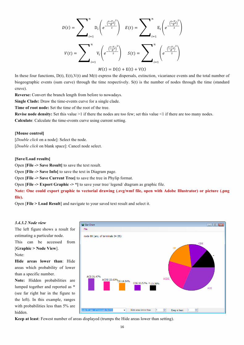
𝑀 𝑡 = D t + E t + V t In these four functions, D(t), E(t),V(t) and M(t) express the dispersals, extinction, vicariance events and the total number of biogeographic events (sum curve) through the time respectively. S(t) is the number of nodes through the time (standard cruve). Reverse: Convert the branch length from before to nowadays. Single Clade: Draw the time-events curve for a single clade. Time of root node: Set the time of the root of the tree. Revise node density: Set this value >1 if there the nodes are too few; set this value <1 if there are too many nodes. Calculate: Calculate the time-events curve using current setting. [Mouse control] [Double click on a node]: Select the node. [Double click on blank space]: Cancel node select. [Save/Load results] Open [File -> Save Result] to save the text result. Open [File -> Save Info] to save the text in Diagram page. Open [File -> Save Current Tree] to save the tree in Phylip format. Open [File -> Export Graphic -> *] to save your tree/ legend/ dtagram as graphic file. Note: One could export graphic to vectorial drawing (.svg/wmf file, open with Adobe Illustrator) or picture (.png file). Open [File > Load Result] and navigate to your saved text result and select it. 3.4.3.2 Node view The left figure shows a result for estimating a particular node. This can be accessed from [Graphic > Node View]. Note: Hide areas lower than: Hide areas which probability of lower than a specific number. Note: Hidden probabilities are lumped together and reported as * (see far right bar in the figure to the left). In this example, ranges with probabilities less than 5% are hidden. Keep at least: Fewest number of areas displayed (trumps the Hide areas lower than setting).
17
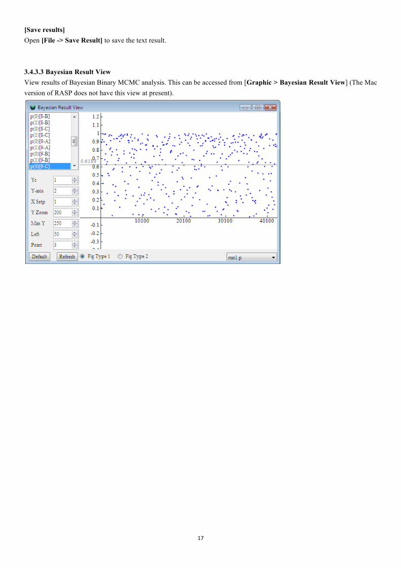
[Save results] Open [File -> Save Result] to save the text result. 3.4.3.3 Bayesian Result View View results of Bayesian Binary MCMC analysis. This can be accessed from [Graphic > Bayesian Result View] (The Mac version of RASP does not have this view at present).
18
4. How to …(back to contents)
All sample files referenced in this manual are in the sample folder.
4.1 How to make Trees data set.
4.1.1 How to obtain trees data set from BEAST. (Back to Top) l Launch BEAUti v*.exe l Select File > Import Alignment and navigate to your NEXUS input file.
(From our sample files, we would select sample1.nex in the Sample folder) (Note: If BEAUti can’t load the NEXUS file then load the file into PAUP and export it use “format=NEXUS” option.)
l Select MCMC panel, set the number of generations the MCMC algorithm will run for. (We set length of chain = 1000000 to do a quick run)
l Click Generate BEAST file… and save your file. (We saved it as samlpe1.xml in sample folder)
l Launch BEAST v*.exe l Enter a Random number seed like 12345 l Choose your BEAST XML input file.
(From our sample files, we would select sample1.nex in the Sample folder) l Run it! l After the program is finished, you will find a .trees file in the same folder of your .xml file.
(In our example, Sample1 .trees is our trees data set.)
4.1.2 How to obtain trees data set from PAUP. (Back to Top) l Use Lset or Pset command set for ML or MP analysis with option “Collapse= NO;” l Define outgroups and root the trees with “roottrees OUTROOT=MONOPHYL;” l Save all of your trees using “format=NEXUS” option.
Important: Trees with polytomies could only be used in Bayesian Binary MCMC and MP analysis!
4.1.3 How to obtain trees data set from other phylogenetic programs. (Back to Top) If you are using Mrbayes, it is helpful to define outgroups and specify rooting before you run mcmc. If you did not define outgroups and specify rooting before the MrBayes run, you can root all trees using PAUP or other available software. You can load the MrBayes output file (*.run.t) as your trees data set once the trees have been rooted. For other phylogenetic programs, there are two methods for making a trees data set: Method 1: l Save the trees as Nexus format from whatever phylogenetic program you are using. Method 2: l Save the trees as PHYLIP format. l Load the trees into PAUP then export the trees use “format=NEXUS” option. Important: Trees with polytomies could only be used in Bayesian Binary MCMC and MP analysis!
19
4.1.4 The bare essentials for the tree file. (Back to Top) Our sample trees file includes considerable amounts of phylogenetic program output, but here is what a trees file must contain. An example, which can be accepted by RASP, is shown to the left.
l Your taxa should have unique labels or names (upper arrow). l Translate your unique taxon names into integers (1- ~) (middle
arrow). These integers are required for the ID field in the RASP program. l Your file should contain one or more phylogenetic trees in set
notation (lower arrow). Many tree generating programs such as PAUP*, MrBAYES, etc. include a lot of extra information within each tree such as branch lengths, likelihood values, and so on. This extra information does not hinder RASP, but it is also not essential. Note: Some programs used to root trees, place the outgroup at the beginning on the tree strong (like the outgroup 3 in the example), others do the opposite, placing the outgroup at the end of the strong. RASP can accept both types of rooting.
l l
4.2 How to make a Final tree.
4.2.1 How to make a final tree by Tree Annotator. (Back to Top) l Launch TreeAnnotator*.exe
l Set Burnin and Posterior Probability l Choose your trees data set as Input Tree File
(In our example, we chose sample\sample1.trees) l Choose Output File
(We saved it as Sample1_Final_Tree.tre in sample folder. Sample1_Final_Tree.tre is our final tree.)
4.2.2 How to make a final tree using PAUP. (Back to Top) l Define outgroups and root the trees with “roottrees OUTROOT=MONOPHYL;” l Export a tree using “savetrees format=NEXUS” commands.
4.2.3 How to obtain a final tree from other phylogenetic programs. (Back to Top) If you are using Mrbayes, you should make the final tree using Tree Annotator or PAUP*. To make a final tree using other phylogenetic programs, there are three methods for making a final tree: Method 1: l Save the tree as Nexus format from whatever phylogenetic program you are using. Method 2: l Save the tree as PHYLIP format. l Load the tree into PAUP then export the tree use “format=NEXUS” option. Method 3: l Make a text tree file by yourself as the following format:
tree=(((((6,((2,4),((9,8),3))),1),(7,11)),10),5); Important: Trees with polytomies could only be used in Bayesian Binary MCMC and MP analysis!
20
4.2.4 The bare essentials of the final tree. (Back to Top) Final tree files may contain various types of commands and information relevant to the program that created them (e.g., #NEXUS, Begin trees;, etc.) An RASP final tree must contain a line of text that looks like: tree=(((((6,((2,4),((9,8),3))),1),(7,11)),10),5); Taxon names must be replaced with integers as shown. The unique integer representing each taxon should be the same as in the trees file. Other types of information in the final tree file may not hinder RASP but are not required.
4.3 How to make Distributions file
4.3.1 How to make a Distributions file. (Back to Top) Name the distributions A, B, C, etc. and specify multiple-area distributions like BD or ACE. Only letters from A to O can be used (Ronquist, 1997, 2001). l Launch RASP l Select File > Load Trees and navigate to your trees data set l Select File > Save Distribution and save it as a .csv file l Open the your saved .csv file in a text editor or Excel l Input the distributions after the species name like this:
or
Note: RASP can tolerate differences in taxon names between the trees file and the distribution file (i.e., Species_01 in your trees file compared to Species01 or Any_name in the taxon or B column). You will receive a warning as below, but you will be allowed to continue. Species_01 is not the same with Any_name! Please examine it before analysis! 4.3.2 How to input distributions in RASP. (Back to Top)
Name the distributions A, B, C, etc. and specify multiple-area distributions like BD or ACE. Letters from A to O must be used (Ronquist, 1997, 2001). l Launch RASP l Select File > Load Trees and navigate to your trees data set l Type your distributions directly into the Distribution column.
l Remember to save the distributions you have entered to a file for use in future analyses. Save the distributions as a .csv file using File > Save Distribution.
21
4.4 Examples
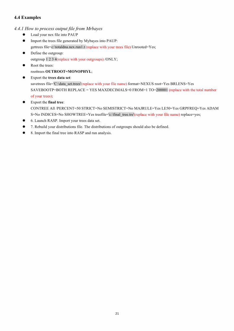
4.4.1 How to process output file from Mrbayes l Load your nex file into PAUP l Import the trees file generated by Mybayes into PAUP:
gettrees file=c:\totaldna.nex.run1.t (replace with your trees file) Unrooted=Yes; l Define the outgroup:
outgroup 1 2 3 4(replace with your outgroups) /ONLY; l Root the trees:
roottrees OUTROOT=MONOPHYL; l Export the trees data set:
savetrees file='C:\data_set.trees'(replace with your file name) format=NEXUS root=Yes BRLENS=Yes SAVEBOOTP=BOTH REPLACE = YES MAXDECIMALS=0 FROM=1 TO=200001 (replace with the total number of your trees);
l Export the final tree: CONTREE All /PERCENT=50 STRICT=No SEMISTRICT=No MAJRULE=Yes LE50=Yes GRPFREQ=Yes ADAMS=No INDICES=No SHOWTREE=Yes treefile='c:\final_tree.tre'(replace with your file name) replace=yes;
l 6. Launch RASP. Import your trees data set. l 7. Rebuild your distributions file. The distributions of outgroups should also be defined. l 8. Import the final tree into RASP and run analysis.
22
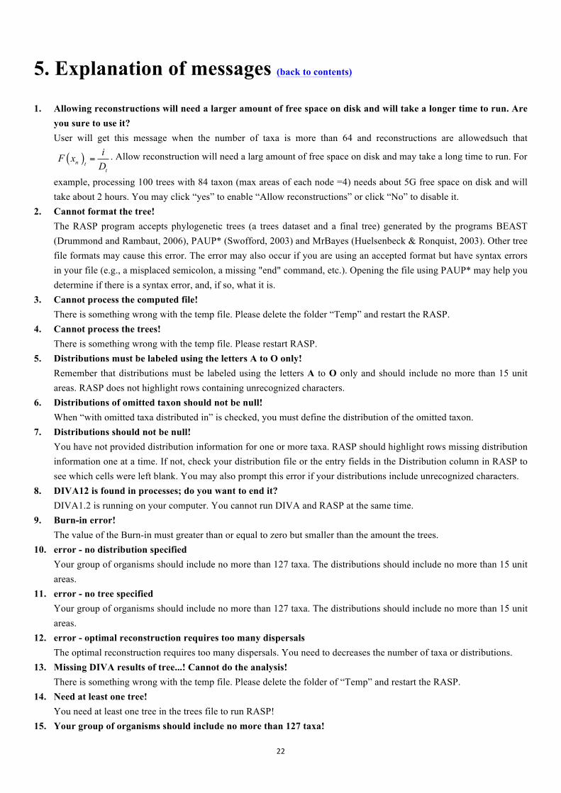
5. Explanation of messages (back to contents)
1. Allowing reconstructions will need a larger amount of free space on disk and will take a longer time to run. Are you sure to use it? User will get this message when the number of taxa is more than 64 and reconstructions are allowedsuch that
( ) n tt
iF xD
= . Allow reconstruction will need a larg amount of free space on disk and may take a long time to run. For
example, processing 100 trees with 84 taxon (max areas of each node =4) needs about 5G free space on disk and will take about 2 hours. You may click “yes” to enable “Allow reconstructions” or click “No” to disable it.
2. Cannot format the tree! The RASP program accepts phylogenetic trees (a trees dataset and a final tree) generated by the programs BEAST (Drummond and Rambaut, 2006), PAUP* (Swofford, 2003) and MrBayes (Huelsenbeck & Ronquist, 2003). Other tree file formats may cause this error. The error may also occur if you are using an accepted format but have syntax errors in your file (e.g., a misplaced semicolon, a missing "end" command, etc.). Opening the file using PAUP* may help you determine if there is a syntax error, and, if so, what it is.
3. Cannot process the computed file! There is something wrong with the temp file. Please delete the folder “Temp” and restart the RASP.
4. Cannot process the trees! There is something wrong with the temp file. Please restart RASP.
5. Distributions must be labeled using the letters A to O only! Remember that distributions must be labeled using the letters A to O only and should include no more than 15 unit areas. RASP does not highlight rows containing unrecognized characters.
6. Distributions of omitted taxon should not be null! When “with omitted taxa distributed in” is checked, you must define the distribution of the omitted taxon.
7. Distributions should not be null! You have not provided distribution information for one or more taxa. RASP should highlight rows missing distribution information one at a time. If not, check your distribution file or the entry fields in the Distribution column in RASP to see which cells were left blank. You may also prompt this error if your distributions include unrecognized characters.
8. DIVA12 is found in processes; do you want to end it? DIVA1.2 is running on your computer. You cannot run DIVA and RASP at the same time.
9. Burn-in error! The value of the Burn-in must greater than or equal to zero but smaller than the amount the trees.
10. error - no distribution specified Your group of organisms should include no more than 127 taxa. The distributions should include no more than 15 unit areas.
11. error - no tree specified Your group of organisms should include no more than 127 taxa. The distributions should include no more than 15 unit areas.
12. error - optimal reconstruction requires too many dispersals The optimal reconstruction requires too many dispersals. You need to decreases the number of taxa or distributions.
13. Missing DIVA results of tree...! Cannot do the analysis! There is something wrong with the temp file. Please delete the folder of “Temp” and restart the RASP.
14. Need at least one tree! You need at least one tree in the trees file to run RASP!
15. Your group of organisms should include no more than 127 taxa!
23
Your group of organisms should include no more than 127 taxa and the distributions should include no more than 15 unit areas in S-DIVA method. You may try to use Bayesian method.
16. Please change your system's number format to English! (ex. 3.14 not 3,14) The decimal symbol of your system caused this problem. Please go to “control panel->Regional and Language Options” and change your "Current format" to English. It is a bug and I will try to fix it in the next release of RASP.
17. Distributions should be Continuous letters! Please alter area … The distributions in Bayesian method must be continuous letters. For instance: Right, ABCDE; Wrong, ACDEF
18. Your group of organisms should include no more than 512 taxa! Your group of organisms should include no more than 512 taxa in Bayesian method.
24
6. References (back to contents)
Alexandre A., Johan A.A.N., Claes P., Isabel S. (2009) Tracing the impact of the Andean uplift on Neotropical plant
evolution. Proceedings of the National Academy of Sciences of the United States of America 106 (24): 9749–9754
Donoghue M.J., Smith S.A. (2004) Patterns in the assembly of the temperate forest around the Northern Hemisphere.
Philosophical Transactions of the Royal Society of London: Biology 359: 1633–1644.
Drummond, A.J. and Rambaut, A. (2006) BEAST v1.4. http://beast.bio.ed.ac.uk/.
Felsenstein, J. (1993) PHYLIP (Phylogeny Inference Package) version 3.5c. Distributed by the author. Department of
Genetics, University of Washington, Seattle.
Harris AJ, Xiang Q-Y. (2009) Estimating ancestral distributions of lineages with uncertain sister groups: a statistical
approach to Dispersal-Vicariance Analysis and a case using Aesculus L. (Sapindaceae) including fossils. Journal of
Systematics and Evolution 47: 349–368.
Huelsenbeck J.P., Ronquist F. (2003) MrBayes 3: Bayesian phylogenetic inference under mixed models. Bioinformatics, 19,
1572–1574.
Lamm K.S., Redelings B.D. (2009) Reconstructing ancestral ranges in historical biogeography: properties and prospects.
Journal of Systematics and Evolution, 47, 369–382.
Nylander J.A.A., Olsson U., Alström P, Sanmartín I. (2008) Accounting for phylogenetic uncertainty in biogeography: a
Bayesian approach to Dispersal–icariance Analysis of the thrushes (Aves: Turdus). Systematic Biology, 57, 257–268.
Ronquist, F. (2001) DIVA version 1.2. Computer program for MacOS and Win32. Evolutionary Biology Centre, Uppsala
University. Available at http://www.ebc.uu.se/systzoo/research/diva/diva.html.
Ronquist, F. (1997) Dispersal-vicariance analysis: A new approach to the quantification of historical biogeography.
Systematic Biology, 46, 195–203.
Ronquist, F. (2001) DIVA version 1.2. Computer program for MacOS and Win32. Evolutionary Biology Centre, Uppsala
University. Available at http://www.ebc.uu.se/systzoo/research/diva/diva.html.