A scanning Kerr microscope with high spatial and temporal resolutions DISSERTATION zur Erlangung des Grades eines Doktors der Naturwissenschaften in der Fakult¨ at f¨ ur Physik und Astronomie der Ruhr-Universit¨ at Bochum 0 fs 1 m m 100 fs 200 fs 300 fs 400 fs 500 fs Dq k [a.u.] von Jie Li aus Chongqing (China) Bochum 2010
Transcript
A scanning Kerr microscope withhigh spatial and temporal resolutions
DISSERTATION
zur Erlangung des Grades eines Doktors der Naturwissenschaften
in der Fakultat fur Physik und Astronomie der
Ruhr-Universitat Bochum
0 fs
1 m�
100 fs 200 fs
300 fs 400 fs 500 fs
��
k[a
.u.]
von
Jie Li
aus
Chongqing (China)
Bochum 2010
Mit Genehmigung des Dekanats vom 10.03.2010 wurde die
Dissertation in englischer Sprache verfasst.
Mit Genehmigung des Dekanats vom 10.03.2010 wurden Teile dieser
Arbeit vorab veroffentlicht. Eine Zusammenstellung befindet
Many people have contributed either directly or indirectly to this study. Without
their helps, supports and encouragements this thesis would not have been possible. I am
obligated to acknowledge here my gratitude.
First and foremost, I would like to thank both Prof. H. Zabel and Prof. T. Eimuller
for offering me the opportunity to join the Junior Research Group Magnetic Microcopy
in the Institute of Experimental Physics IV. As the first PhD student in this new group
starting with an empty laboratory, there have been a lot of technical, scientific as well as
administrative difficulties which we did not expected. This work would have been very
difficult or even impossible without their patience, words of encouragement and advice.
Their enthusiastic attitudes toward scientific researches and precise manners of working
are excellent examples I should follow.
I would also like to thank Prof. Dr. Kurt Westerholt and Prof. Dr. Ulrich Kohler
for their suggestion concerning thesis writing and preparation of the oral defence. In
addition, I am also grateful to PD Dr. Oleg Petracic for the introduction of micromagnetic
simulation using finite element method. I have benefited greatly from the comments and
suggestions of Dr. Olav Hellwig from Hitachi Global Storage Technologies concerning the
possible application of this microscope in the patterned media storage industry.
Grateful acknowledgement is dedicated to my colleagues in the institute. Thanks
to Min-Sang Lee, Dr. We He and Stefan Buschhorn for many insightful discussions
concerning magnetization dynamics. Further thanks to Dipl. Phys. Philipp Szary. Most
of the Permalloy samples are produced by him under the supervision of PD Dr. Oleg
Petracic. In addition, I would like to thank Frank Brussing for discussion about the
detection of Kerr signal using the photo-elastic modulator. In particular, I would like to
thank Bjorn Redeker, the technician of our group. He has designed, constructed most of
the mechanic components of this microscope. I would also like to thank other technicians
in the mechanical workshop of this institute, Peter Stauche, Horst Glowatzki and Jorg
Meermann, for their support. I am especially grateful to Dennis Schopper, the computer
administrator, for many useful suggestions about the controlling software of this setup.
The last but not the least, I would like to add personal thanks to Petra Hahn, Dr. Hui
He, Dr. Dirk Sprungmann, Gregor Nowak, Alexandra Schumann and all other students
and researchers in our institute.
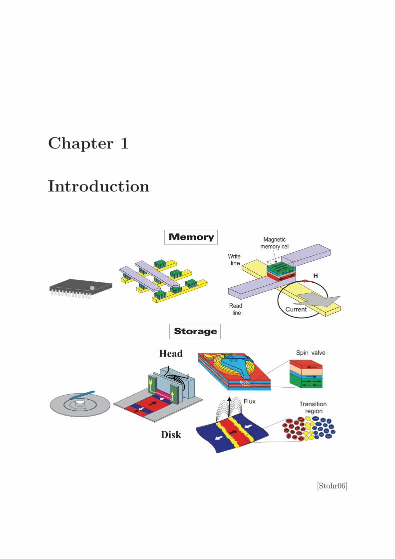
Chapter 1
Introduction
valve
m c
l
rT
[Stohr06]
1.1 Historical Review 2
“Technology has advanced more
in the last thirty years than
in the previous two thousand.
The exponential increase
in advancement will only continue.”
– Niels Bohr
1.1 Historical Review
The magnetic materials were observed long time ago, possibly even before the beginning
of the civilization. According to the written documents that have been discovered, Thales
of Miletus (634 - 546 BC) is the first person who clearly described the phenomenon that
the “lodestone” attracts iron. The chemical composition of such mineral is Fe3O4. It is
possibly magnetized by the earth’s magnetic field during the cooling process of hot lava.
The Chinese ancient scholar Guan Zhong (725 - 654 BC) has also made similar descrip-
tion regarding lodestone in his work of Guanzi, an encyclopedic compilation of Chinese
philosophical materials [Song87] 1. It was called “ci shi”, the “loving stone”, in that book
as well as in many other Chinese literatures in the following centuries.
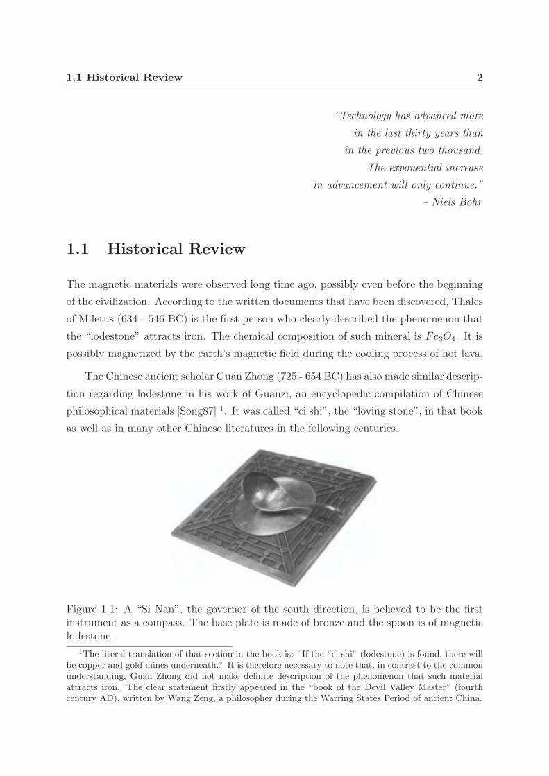
Figure 1.1: A “Si Nan”, the governor of the south direction, is believed to be the firstinstrument as a compass. The base plate is made of bronze and the spoon is of magneticlodestone.
1The literal translation of that section in the book is: “If the “ci shi” (lodestone) is found, there willbe copper and gold mines underneath.” It is therefore necessary to note that, in contrast to the commonunderstanding, Guan Zhong did not make definite description of the phenomenon that such materialattracts iron. The clear statement firstly appeared in the “book of the Devil Valley Master” (fourthcentury AD), written by Wang Zeng, a philosopher during the Warring States Period of ancient China.
1.1 Historical Review 3
The first practical application of the magnetic material was the directional pointer,
invented during the Qin dynasty (221-206 BC), as shown in Fig. 1.1. This prototype of
compass was used as directional pointer for “feng shui” 2, the technique used not only to
arrange location and direction of houses and the geometrical orientation and configuration
of the objects inside, but also to select locations and orientations of graves for those who
passed away. The latter is still commonly practiced in rural area of China nowadays and
it is believed that it will bring great fortune to the descendants if the tombs are located
on top of “dragon veins”.
The application of magnetic directional pointer in “feng shui” has hardly made any
contribution to the development of the modern civilization, even through it is still com-
monly practiced in East Asia. It is believed that this technique was firstly employed for
the navigation in China at end of 11th century. Few decades later, it was used in Europe
as well. With out the magnetic compass, the Age of Exploration wouldn’t haven been
possible and our world might have developed in a totally different way.
The scientific understanding of the magnetism started much later, together with
the development of the modern industrialization. A large number of researchers, such
as Carl Friedrich Gauss, Hans Christian Ørsted and Andre Marie Ampere, have made
contribution but the most critical breakthrough of magnetism, or electromagnetism in
general, was made by the experimentalist Michael Faraday together with the theoretician
James Clerk Maxwell.
Faraday has discovered the electromagnetic induction and the Faraday Effect, the
change of the polarization of the light when propagating through a magnetized material.
The same magneto-optical effect in reflection also exists and was discovered later by
John Kerr. As an experimental physicist, Faraday did not summarize this discovery
with a solid mathematical description. However, this was done by Maxwell in this book
“Treatise on Electricity and Magnetism”. There, he concluded that light is indeed a form
of electromagnetic wave with a velocity of c = 1/√
ε0μ0 in vacuum. It is worthwhile to
note that this equation is true for any inertial frame of reference which means the c is
always a constant. Such a prediction contradicted classical mechanics and the explanation
of this problem leads to the development of the theory of special relativity.
2In ancient Chinese philosophy, there are “magnetic fields” around all objects which generate at-tractive and repulsive (positive and negative) forces between them. The “feng shui” is a technique tooptimize their locations in order to reach the equilibrium.
1.2 Magnetic Recording Technology 4
1.2 Magnetic Recording Technology
Scientific study in magnetism has made two major contributions to the modern technol-
ogy: the production of electricity using high energy product permanent magnets and the
magnetic data storage in information technology. The concept of magnetic recording was
firstly introduced by Oberlin Smith as early as 1888. A few years later, Valdemar Poulsen
filed the patent of the telegraphone, the first working model of magnetic storage device.
1.2.1 Magnetic Core Memory
An Wang, a Harvard physicist and the co-founder of the computer company Wang Labo-
ratories, was the first person to demonstrate the prototype of modern magnetic recording
device: the magnetic core memory. This technique was widely used in IT industry in the
60s, replacing both the drum memory and the vacuum tube memory. The production of
the this type of memory requires manual operations of the fine motor control under mi-
croscopes to assemble core arrays. The lifetime of the core memory was relatively short:
it was replaced by integrated silicon RAM chips in the 1970s.
It is also important to note that magnetic core memory is indeed a random access
computer memory, in which each bit can be read and write independently. Another
important feature is its non-volatile characteristics. Since the polarity of the magnetic
field of the cores represents the bit information, the data are retained even if the power
is cut off. Unlike silicon RAM chips, it is also relatively unaffected by electromagnetic
pulse (EMP) or radiation. Because of these advantages, magnetic core memory was still
used in many businesses many years after the silicon RAM became available.
1.2.2 Magneto-optical Drive
Magneto-optical drive is another type of magnetic storage, which was introduced at the
end of the 1980s. In contrast to magnetic core memory, it is a sequential access memory
where the data can only be read and write in sequence. The rotating disc consists of a
magnetic layer covered by protecting coatings. During the writing process, a laser beam
with high power is focused and heats the magnetic layer up to the Curie point. The
magnetization in the focus is reversed by an electromagnet located on the opposite side of
the platter. To read out the data, the power of the laser is decreased and the orientation
1.2 Magnetic Recording Technology 5
(A) (B)
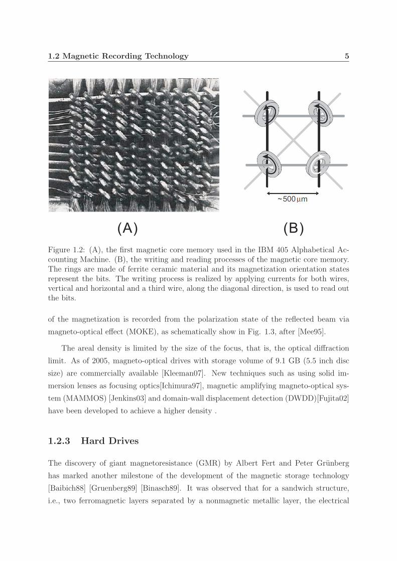
Figure 1.2: (A), the first magnetic core memory used in the IBM 405 Alphabetical Ac-counting Machine. (B), the writing and reading processes of the magnetic core memory.The rings are made of ferrite ceramic material and its magnetization orientation statesrepresent the bits. The writing process is realized by applying currents for both wires,vertical and horizontal and a third wire, along the diagonal direction, is used to read outthe bits.
of the magnetization is recorded from the polarization state of the reflected beam via
magneto-optical effect (MOKE), as schematically show in Fig. 1.3, after [Mee95].
The areal density is limited by the size of the focus, that is, the optical diffraction
limit. As of 2005, magneto-optical drives with storage volume of 9.1 GB (5.5 inch disc
size) are commercially available [Kleeman07]. New techniques such as using solid im-
mersion lenses as focusing optics[Ichimura97], magnetic amplifying magneto-optical sys-
tem (MAMMOS) [Jenkins03] and domain-wall displacement detection (DWDD)[Fujita02]
have been developed to achieve a higher density .
1.2.3 Hard Drives
The discovery of giant magnetoresistance (GMR) by Albert Fert and Peter Grunberg
has marked another milestone of the development of the magnetic storage technology
[Baibich88] [Gruenberg89] [Binasch89]. It was observed that for a sandwich structure,
i.e., two ferromagnetic layers separated by a nonmagnetic metallic layer, the electrical
1.2 Magnetic Recording Technology 6
Figure 1.3: Schematic layout of the magneto-optical drives. Note that a balanced detec-tion technique is used to record the MOKE signal, which consists of a polarizing beamsplitter, two photodiodes and an operational amplifier for the subtract function.
resistance changes dramatically when the magnetization orientation of one magnetic layer
is reversed. The explanation is the different scattering rate for the electrons with opposite
spins. Since GMR is generally a large effect (80% in multilayer systems), it has been
used extensively to build highly sensitive devices to detect slight change of the external
magnetic field and has fueled the emergence of a new field of electronics called spintronics.
Several years after the discovery of the GMR, similar effect was observed in the
multilayer systems where the metallic spacing layer is replaced by an insulator layer
[Moodera95]. In this case, the effect is due to the tunneling probability difference of
the spin up and spin down electrons. Therefore it is solely a quantum effect and is
named as tunneling magnetoresistance (TMR). The relative change of resistances at room
temperature up to several hundred percent were observed [Parkin04] [Yuasa04]. The
record at the moment is 600% at room temperature and 1144% at 5 K, observed in the
CoFeB/MgO/CoFeB junctions[Ikeda08].
The operation principle of the modern hard drive is described in the Fig. 1.4. The
magnetic recording material is deposited on a flat substrate. Due to their different op-
eration mechanism, the read and write heads are separated. In order to write a bit, a
short current pulse is applied to the write head, generating a short magnetic field pulse
1.2 Magnetic Recording Technology 7
“Ring”
N S N S N S S NS NS N
RecordingMedium
Magnetizations
P2Shield 2P1
Inductive WriteElement
V write
N S S NN S
sensor
Figure 1.4: Schematic representation of the read and write process of the modern longi-tudinal recording hard drives, after [Hitachi].
to reverse the magnetization of the small element underneath. The magnetic recording
medium is made of materials with preferred magnetization directions, i.e., magnetocrys-
talline anisotropy, which means the magnetization direction tends to be spontaneously
aligned in one direction or the opposite direction, representing the “1” or “0” of a bit.
The spatial size of the element, i.e., the areal density, is the most critical parameter of this
technology. However, due to the slow reading process limited by the mechanical motion
of the heads, the magnetization dynamics occurs during the reversal is totally neglected.
A GMR or TMR sensor, schematically illustrated as an analog meter as shown in Fig.
1.4, is used as the read head to detect the direction of the stray field from the magnetic
recording medium. The stray field is large enough to reverse the magnetization direction
of the free layer of the head and hence alter the resistance of the head. This change is
transferred to an analog voltage output signal representing the information recorded on
the magnetic element.
Due to the ultra high sensitivity of GMR or TMR sensors, the size of the “bit” on the
rotating platters can be greatly reduced and hence the areal density of hard drives has
been increased drastically over the last decade, as summarized in the Fig. 1.5 [Hitachi].
At the beginning of 2009, Seagate introduced the hard drive with a areal density of 329
Gb/inch2 to the commercial market [Seagate09]3. In the laboratories, 612 Gb/in2 has
already been demonstrated [Tanahashi09]. With the size of the “bit” becomes smaller
3With this areal density, the increase factor shown in Fig 1.5 is now more than 300 million, insteadof 35 million.
1.2 Magnetic Recording Technology 8
60 70 80 90 100 110
Production Year
1E-3
1E-2
1E-1
1E+0
1E+1
1E+2
1E+3
1E+4
1E+5
1E+6
Are
alD
ensi
ty M
egab
its/in
2
HGST Disk Drive ProductsIndustry Lab DemosHGST Disk Drives w/AFCDemos w/AFC
HGST Areal Density Perspective
1st MR Head
1st GMR Head
2000 10
Ed Grochowski
60% CGR
Ultrastar 146Z10
Deskstar 180GXP
100% CGR
Corsair
Deskstar 16GP
Travelstar 30GNMicrodrive II
1st AFC Media
Future ArealDensityProgress
Travelstar 80GN
PerpendicularRecording
Superparamagneticeffect
105
104
103
102
106
10
1
10-1
10-2
10-3
25% CGR
IBM RAMAC (First Hard Disk Drive)
1st Thin Film Head3375
35 Million XIncrease
Figure 1.5: Exponential growth of the hard drive areal density, after [Hitachi]. From1957 to 2007, the density has been increased by a factor of 35 million. In the 1990s, theincrease rate was 60% per year and was accelerated to 100% per year in the 2000s.
and smaller, the hard drive is now approaching the fundamental physical limit of super-
paramagnetism, in which random reversal of the magnetization occurs under the effect
of thermal fluctuation. Perpendicular recording was used to replace the conventional
longitudinal recording in order to push this limit to about 1 Tb/inch2 [Hitachi07] and
other techniques, such as heat-assisted magnetic recording (HAMR) [Seigler08], bit pat-
terned magnetic recording (BPMR) [Schabes08] and microwave assisted magnetic record-
ing (MAMR) [Zhu08] are currently under development.
In contrast to the spectacular development of the density, there has not been any
significant improvement of the hard drive’s seek time, the delay for the head to move the
correct location on the platter to read or write the data. This is a general disadvantage
for sequential access memories where one single head is used to access all bits on the
recording media. It has been improved to from about 100 ms to 20 ms in the 1980s by
replacing step motor with voice coil for the head positioning and remains nearly the same
1.2 Magnetic Recording Technology 9
for the current hard drives. Another weakness of the hard drive is the relatively slow data
transfer rate, which is limited to 50-100 MB/s by the rotational speed of the platter and
the density. This data transfer speed is much slower than that of the dynamic random
access memory (DRAM), causing long and frustrating booting process of a computer.
1.2.4 Magnetoresistive Random Access Memory
Figure 1.6: Schematic illustration of the magnetoresistive random access memory (MTJdesign) [Cowburn03]. The bits are accessed with the grid of word and bit lines. Theinsert is the detailed structure of a single magnetic element: the bit is stored as themagnetization orientation of the free layer and is readout by the resistance difference ofthe MTJ.
The magnetoresistive random access memory (MRAM) is a new type of RAM which
has been under development since the 1990s [Daughton92, Daughton97]. In this technol-
ogy, a bit is stored as the magnetization orientation of a small size magnetic element and
therefore it is non-volatile because no electricity is required to maintain the information,
as shown in Fig. 1.6. This concept is very similar to the magnetic core memory but it has
a much higher areal density. There are mainly three types: the pseudospin-valve design,
the magnetic tunneling junction (MTJ) design and the vertical current perpendicular to
plane (CPP) spin valve GMR design.
In the pseudospin-valve design, a single element consists of two ferromagnetic layers
and a non-magnetic conductive spacing layer in between. The top magnetic layer has a
lower switching field thus is called soft layer and the bottom layer with higher switching
field is referred to as the hard layer. The bit, “1” or “0”, is stored as the magnetiza-
tion direction of the hard layer and is readout by the soft layer using GMR effect. In
the MTJ design, a MTJ is combined with a synthetic antiferromagnet (SAF) and an
1.3 Faster and Smaller 10
antiferromagnetic layer. The bit is stored as the direction of the magnetic moment of
the top layer in MTJ, called as the storage layer. The bottom layer of MTJ works as a
reference layer. It is important to note that one CMOS transistor is needed to read out
each element. One crucial problem of these two designs is the relatively large spacing
between two elements, restricted by the stray field generated by the magnetic layers.
The solution is a new design, the vertical magnetoresistive access memory (VMRAM),
in which a stable magnetization flux closure in the element is realized by using a circular
magnetization mode [Zhu03]. The read and write operation of this design is very similar
to the pseudospin-valve memory.
1.3 Faster and Smaller
As the size of the “digital universe” will increase explosively in the foreseeable future, from
281× 1018 Bytes in 2007 (45 GB per person) to about 1.8× 10²¹ Bytes in 2011 (290 GB
per person) [emc08], it is essentially important for the data storage industry to maintain
a fast development of the capacity of the hard drives. A larger capacity with the same
physical dimension means a higher areal density or a smaller magnetic element size. Over
the last decade, this need from the industry has fueled the fundamental research in the
scientific community to obtain knowledge about the magnetic properties of the structures
on a nanometer scale. Experimental techniques, such as magnetic transmission x-ray
microscopy (MTXM) [Fischer98], x-ray photoemission electron microscopy (X-PEEM)
[Scholl02] and magnetic force microscopy (MFM) [Rugar90] with high spatial resolution
have been developed for this purpose.
On the other hand, with the introduction of the MRAM concept, it is possible to push
the read and write speed of the magnetic storage technique into the GHz regime, i.e., to
access times in the ns regime. This requires a detailed knowledge of the magnetization
dynamics on time scale of ps. The mechanism behind spin precession and damping is
therefore essential. In line with this industrial and scientific need, experimental techniques
using the pump-and-probe (excitation-and-detection) concept have been introduced. The
basic principle is to excite the magnetic system in a certain way and detect the response
of the system after a time delay δt. The excitation methods can be generally categorized
into three types, as shown in Fig. 1.7:
• H(t): The perturbation is induced by a magnetic field pulse and generated either
1.3 Faster and Smaller 11
by a electronic pulser or by current switch illuminated by a laser pulse.
• T (t): Thermal excitation focuses a laser pulse directly to the magnetic sample.
• S(t): Spin-selective excitation uses a circularly polarized laser pulse.
H( t )
T( t )
S( t )
s +
H( t )
T( t )
S( t )
s +
laser heating
magnetic perturbation
spin-selectiveexcitation
Figure 1.7: Schematic illustration of the three excitation techniques, after [Koopmans03].
Similarly, the detection of the induced magnetization dynamics can be realized by
different magnetic imaging methods, such as magneto-optical Kerr effect (MOKE). How-
ever, it is important to note that in order to study the magnetization dynamics on the
ultrafast timescale (below 100 ps), which is one of the most interesting topics in the
current magnetism community, the time scales of both excitation and detection are es-
sential parameters. For this reason, the all-optical pump-and-probe MOKE technique
[Beaurepaire96], in which the magnetic system is excited and detected by femtosecond
laser pulses, is currently the best choice to study the ultrafast magnetization dynamics.
In contrast, other techniques, such as magnetic field pulse excitation and MOKE detec-
tion [Freeman96] or femtosecond laser excitation and x-ray detection [Eimuller07], are
only able to access the magnetization dynamics in the 100 ps regime. Fig. 1.8 is a brief
summary of various experimental techniques on different timescales.
The main part of this work is to design, construct and test a femtosecond time-
resolved scanning Kerr microscope using an all-optical pump-and-probe technique. In
contrast to other all-optical time-resolved MOKE setups, this microscope provides not
only a high temporal resolution but also a high spatial resolution. A general purpose
equipment controlling and data recording program was designed initially for this setup.
Due to the universal design principle, it was later adapted for other experimental setups.
This thesis is organized in the following manner:
1.3 Faster and Smaller 12
Exchange interaction
Spin-orbitcoupling
1 fs
1 ps
10 fs
100 fs
100 as
10 ps
100 ps
1 ns
Spin precession
Gilbert damping
10 ns Thermal activation
Spin lattice relaxation time
Electron lattice relaxation time
Ti:Sapphire laser oscillator
Electronic pulsers
single shot Kerr microscopy 10 ns
wide-field stroboscopicKerr microscopy 25 ps
Pump-probe scanningKerr microscopy
High gain higher harmonics generation (HGHG) of laser: 100 as soft x-ray pulses
single cyclepulses: 2.5 fs
electron
lattice spinMTXM, X-PEEM
Figure 1.8: Temporal resolution of different techniques and the corresponding magneti-zation dynamics, after [Stohr06] [Eimueller06].
1.3 Faster and Smaller 13
Chapter 2 will give a short introduction of the relevant magnetic concepts which are
needed for this thesis. Different interactions in the magnetic system and corresponding
energies will be discussed.
Chapter 3 will firstly provide a brief description of the general magnetization dy-
namics, described by the Landau-Lifshitz-Gilbert equation. Following will be a more
detailed discussion of the magnetization dynamics induced by optical excitation with
ultrashort laser pulses, the technique used for this experimental setup.
Chapter 4 contains the elaborated information of the hardware configuration of this
microscope the details of the general purpose equipment control and data acquisition
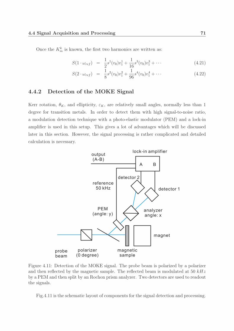
software. The detection of the modulated MOKE signal is relatively complicated and
therefore will be discussed in detail.
Chapter 5 summarizes the result of this work. The temporal and spatial resolution
of this microscope is experimentally estimated. The data from different magnetic sample
will be presented.
Chapter 6 presents the a summary and an outlook. Several additional features of
the microscope are proposed and some technical issues which need to be solved are also
discussed.
Chapter 2
Basics of Magnetism
H
Hd
Hs
B M
[Stohr06]
2.1 Magnetic Interaction and Energy 15
“In science one tries to tell people,
in such a way as to be understood by everyone,
something that no one ever knew before.
But in poetry, it’s the exact opposite.”
– Paul Dirac
2.1 Magnetic Interaction and Energy
The origin of magnetism is the magnetic moments of atoms and molecules under the effect
of the symmetry and the orientation of their electron orbits. In solids, the magnetic
moments are coupled in various ways which gives rise to a cooperative motion that is
very different from the situation where the moments are isolated from each other. The
coupling between the moments has many different mechanisms and this leads to a rich
diversity of the magnetic properties in solids. The magnetic materials can be categorized
into several types, depending on the way they interact with the external magnetic field,
such as diamagnetism, paramagnetism, ferromagnetism or ferrimagnetism. Because in
this work only ferromagnetic materials are involved, the other types of magnetic material
will not be included here, but most text books regarding magnetism, such as [Stohr06],
[Blundell01] and [Aharoni00], give a detailed description of these materials.
The most important character of ferromagnetism is the non-vanishing spontaneous
magnetization observed below a certain temperature, the Curie temperature Tc without
applying an external field. This suggests that their magnetic moments are naturally
aligned by some underlying interactions between them. There are two parts of the electron
magnetic moment, the orbital moment and the spin. The magnitude of the magnetization
M(r) inside a ferromagnet is equal to a constant, the saturation magnetization Ms at all
locations, but the direction is not. This direction is denoted as a magnetic unit vector
m(r) = M(r)/Ms and is named reduced magnetization.
In this section a general summery of the magnetic interactions will be introduced,
detailed description of ferromagnetism is discussed afterward.
2.1 Magnetic Interaction and Energy 16
2.1.1 Exchange Interaction
The exchange interaction is the strongest magnetic interaction (few eV) and it is the origin
of the magnetic ordering, i.e., the parallel or the antiparallel alignment of the spins. It
is a purely quantum mechanical effect and the result of the Pauli Exclusion Principle
and the electrostatic interaction. Theoretical treatment of this interaction requires the
modification of the conventional Schrodinger equation, which does not consider the spin
system. The relativistic Dirac equation is needed for this purpose.
However, if the velocity is small compare to the speed of light, approximation can be
made and a simple term with spin is added to the Schrodinger equation. This is called
the time-independent Pauli equation:
[He + Hs]ψ(r, t) = Eψ(r, t) (2.1)
where He is the Hamiltonian for an atom at the origin with nuclear charge qn = Ze
and the electrons with charge qe = −e:
He =N∑
i=1
(pi
2
2me
− Ze2
4πε0 |ri|) +∑i<j
e2
4πε0 |rj − ri|︸ ︷︷ ︸Coulomb interaction
(2.2)
The last term of this equation is the Coulomb interaction between the electrons and
it gives rise to the exchange interaction.
Hs includes the non-relativistic expression of the spin energy into the original Schrodinger
equation and it is the origin of the spin-orbit interaction:
Hs =e�
me
S · B∗ (2.3)
where S is the spin and B∗ is the origin of the magnetic induction.
In the Heisenberg model, the exchange interaction is described by a parameter Jij
and the effective Hamiltonian can be written as:
Hheisenberg = −∑ij
JijSi · Sj (2.4)
2.1 Magnetic Interaction and Energy 17
where Jij is the exchange constant or the exchange integral between the ith and jth
spin. If Jij > 0, the parallel alignment of the spins is energetically favorable and it
gives rise to the ferromagnetic coupling. On the other hand, when Jij < 0, the spins are
antiparallelly aligned and the coupling is antiferromagnetic, as shown in the following
figure:
(a) (b)
Figure 2.1: Two types of magnetic ordering caused by the exchange interaction. (a)ferromagnetism and (b) antiferromagnetism.
The exchange interaction decreases rapidly by increasing the distance between the
atoms. For this reason, approximation is made that Jij = J is a constant for the nearest
neighbor spins and 0 otherwise. In this case, the value of J can be derived from the Weiss
classical molecular field theory:
J =3kTC
2zS(S + 1)(2.5)
where z is the number of nearest neighbors and Tc is the Curie temperature.
It is important to note that, the Heisenberg model is only valid for localized spins.
However, in ferromagnetic solids, the electrons can be either localized, e.g., 4f-metals, or
delocalized, e.g., 3d-metals. If the effect of the delocalized conducting electrons can not be
neglected, the Heisenberg model is not sufficient and thus different theoretical approaches
are needed [Aharoni00]. It is therefore necessary to take both parts, the localized electrons
and the conducting electrons, i.e., the band structure, into consideration [Blundell01].
Since the spins are delocalized, the simplest model where only the exchange interac-
tions between the nearest neighbors are considered is also not enough. A better picture
is that within a certain length scale, the exchange interaction between all the spins are
taken into account. This scale, called exchange length, is surely material dependent and
2.1 Magnetic Interaction and Energy 18
can be written as [Miltat02]:
Λ =
√2A/μ0Ms
2 (2.6)
where A is proportional to the exchange constant and known as the exchange stiffness.
Its value depends on the system temperature. At Curie temperature, Tc, A is zero. Ms
is the saturation magnetization. Together with other properties, Λ of typical magnetic
materials is listed in the following table [Aquino04]:
Material μ0Ms A ΛUnit [T] 10−11[J/M] [nm]Fe 2.16 1.5 2.8Co 1.82 1.5 3.4Ni 0.62 1.5 9.9
Permalloy 1.0 1.3 3.2
Table 2.1: Properties of several ferromagnetic materials.
For typical ferromagnetic materials, Λ is in the order of several nm and one considers
the magnetization to be spatially uniform within this range. Since this length is relatively
small, the continuum approximation can therefore be made and the lattice structure, i.e.,
the discrete nature of the solids, is neglected and the exchange energy is simplified to a
integral:
Eexchange = A
∫V
[(∇mx)2 + (∇my)
2 + (∇mz)2]d3r (2.7)
now the material dependent characters of the exchange interaction are described by
the exchange stiffness constant A, which can be obtain from Weiss molecular theory:
A =2JS2
a(2.8)
where a denotes the lattice constant.
The ground state of the magnetic system, i.e., the state with the lowest exchange
energy, is therefore a state where all spins are parallelly aligned for ferromagnetic materials
or antiparallelly aligned for ferromagnetic materials. Any deviation from this alignment
will increase the gradient of the magnetic moment and hence elevate the exchange energy.
2.1 Magnetic Interaction and Energy 19
2.1.2 Zeeman Interaction
The interaction between the external magnetic field H and the magnetic moment m is
called the Zeeman interaction. This interaction causes an energy contribution to the total
energy of a magnetic system:
Ezeeman = −μ0Ms
∫V
m · Hd3r (2.9)
The ground state is therefore the state where all m are aligned parallel to the external
field.
Zeeman interaction is the mechanism behind the practical use of magnetic materials.
It is used to align the magnetization of the iron needles of a compass. The modern hard
drive also uses the Zeeman effect to write information on the magnetic recording medium.
2.1.3 Spin-Orbit Interaction
Spin-orbit interaction is the coupling between the spin S with the orbital angular mo-
mentum L, producing a new total angular momentum J = S + L. Although the energy
of this interaction is much smaller (10 to 100 times) than the exchange interaction, it is
still very important. This interaction creates the orbital magnetism and couples the spin
system to the lattice system, which allows to the energy and momentum transfer between
two systems. It is also the reason of the magnetocrystalline anisotropy.
As shown in the Pauli equation 2.1, the term Hs that gives rise to the spin orbital
interaction is written as:
Hs =e�
me
S · B∗ (2.10)
The B∗ is the magnetic induction caused by the relative motion of the electrons and
the nucleus. If the inertial frame of reference is chosen so that the electron is at rest, the
nucleus will spin around the electron, generating a magnetic induction:
B∗ = −υ × E
2c2(2.11)
2.1 Magnetic Interaction and Energy 20
The Hamiltonian of the spin-orbital interaction is expressed as:
Hso = ξnl(r)S · L (2.12)
with ξnl defined as
ξnl(r) =e�2
2me2c2
1
r
dΦ(r)
dr(2.13)
where Φ(r) denotes the electrostatic potential of the nuclear charges. The expectation
value of this term:
ζnl = 〈ξnl(r)〉 (2.14)
is called the spin-orbital constant. For the 3d metals, the value of this constant is in
the order of 10-100 meV and is much larger for rare earth metals [Cowan81].
The magnetostatic energy caused by this interaction is called spin-orbit energy and
is given by:
Espin - orbit = − e2
4πε0m2ec
2r3L · S (2.15)
Magneto-Crystalline Anisotropy
The spin-orbit energy expressed in equation 2.15 can also be explained by the energy
difference between the situation that S is aligned parallel to L and the situation that
they are perpendicular. If the orbital moment has a preferred direction, caused by the
interaction with the lattice system, the spin S is also locked to this direction. This is
the origin of the magneto-crystalline anisotropy and the magnetization has therefore a
preferred direction with lowest energy (easy axis) and a direction with highest energy
(hard axis). The magneto-crystalline anisotropy is defined as the difference of these two
There are several type of magnetocrystalline anisotropies: cubic, orthorhombic and
uniaxial [Hubert00]. In a polycrystalline system, an uniaxial anisotropy can be induced
by applying an external field during the film deposition. An example is the NiFe ferro-
magnetic system. Cubic anisotropy is observed for Fe and Ni. In a perfect single crystal,
the direction of the easy axis is the same at all locations. However for a polycrystalline
system this direction is different at different points, depending on the lattice orientation.
Considering the first case, the anisotropy energy can be expressed by a Taylor expansion
of the magnetic moment, m = (m1, m2, m3) [Hubert00]. If the system has an uniaxial
anisotropy with an anisotropy axis along the z direction, the anisotropy energy is given
by:
Eanisotropy =
∫V
Ku1(1 − m2z) + Ku2(1 − m2
z)2d3r (2.17)
where K is the anisotropy constant and V is volume of the system. The sign of Ku1
determines the direction of the easy axis:
• if Ku1 > 0, the easy axis is along the z direction.
• if Ku1 < 0, the easy axis is perpendicular to the z direction.
For rare earth permanent magnet materials, the uniaxial anisotropy is very large, in
the order of 107 J/m3.
Concerning a cubic anisotropy, this energy is written as:
Eanisotropy =
∫V
[Kc1(m2xm
2y + m2
ym2z + m2
xm2z) + Kc2m
2xm
2ym
2z]d
3r (2.18)
Kc1 and Kc2 are the material dependent anisotropy constants [Hubert00]. The value
of Kc1 is of the order of ±104 J/m3. A positive sign means < 100 > is the easy axis and
a negative sign means < 111 > is the easy axis.
2.1.4 Magnetostatic Energy
The origin of the magnetostatic energy is the interaction between the magnetic moments
and the field they generate by themselves. It causes the magnetization structures on a
2.1 Magnetic Interaction and Energy 22
length scale much larger than the atomic distance. Starting from the Maxwell’s equation:
∇ · B = 0
B = μ0(H + M)(2.19)
This gives rise to the relation that:
∇ · H = −∇ · M (2.20)
Considering the effect of the external current:
∇× H = ja (2.21)
From this, one can decompose the H into two parts: the applied field Ha caused by
the current ja and the magnetostatic field, also called demagnetization field Hd, from the
divergence of the magnetization ∇ ·M. Therefore, the demagnetization field is given by:
∇× Hd = 0
∇ · Hd = −∇ · M(2.22)
This shows that the divergence of the Hd is opposite to the divergence of the mag-
netization M. Inside the magnetic sample, Hd is pointed to the opposite direction of
the internal magnetic field, which is the reason why it is named demagnetization field.
Outside the magnetic sample, this field is normally referred to as the stray field. The
energy caused by this interaction is expressed as:
Ed =1
2μ0
∫all space
Hd2d3r = −1
2μ0Ms
∫the sample
m · Hdd3r (2.23)
This energy is positive in all cases, shown by the first term of this equation (Hd2 > 0),
which means the magnetic system tries to arrange the magnetization distribution m in
such a way that this energy is minimized. The demagnetization energy in the equilibrium
state is normally calculated by means of numerical simulation, which is a very time-
consuming process since this is a long range interaction and all discrete elements are
involved.
2.1 Magnetic Interaction and Energy 23
Because ∇ × Hd = 0, a scalar potential Φd can be defined: Hd = −∇Φd. This
potential can be decomposed into two parts, the volume and the surface part:
Φd(r) =Ms
4π
⎛⎝∫
V
ρV (r′)|r′ − r|d
3r +
∫S
σS(r′)|r′ − r|d
2r
⎞⎠ (2.24)
where the volume charge density and surface charge density are given by (n denotes
the outward surface normal) [Hubert00]:
ρV (r) = −∇ · mσS(r) = m · n
(2.25)
Therefore, the demagnetization energy consists of a volume integral and a surface
integral:
Ed = μ0Ms
⎛⎝∫
V
ρV (r)Φd(r)d3r +
∫S
σS(r′)Φd(r)d2r
⎞⎠ (2.26)
From this equation, the demagnetization is proportional to the surface and the volume
charge densities. Therefore, the system tends to reach a state with less surface and volume
charges, which is called pole avoidance principle.
It is very important to note that for a arbitrary shape magnetic sample, the demag-
netization field can be very complicated. To simplify the calculation, the magnetometric
demagnetization tensor N is defined:
Hd(r) = −N(r) · M(r) (2.27)
N is normally a function of the position r. For a ellipsoidal geometry [Blundell01],
it is a constant and can be diagonalized if m is along a principle axis of the ellipsoid.
Because the demagnetization energy is directly connected to the shape of the magnetic
sample, it is also named shape anisotropy Ks .
Both the magnetocrystalline anisotropy and the shape anisotropy contribute to the
total magnetic anisotropy. As shown in [Stohr06], in case of a thin film with uniaxial
anisotropy, the easy axis of the magnetization is a result of the competition between the
2.1 Magnetic Interaction and Energy 24
magnetocrystalline anisotropy (Ku) and the shape anisotropy (Ks):
• if Ku + Ks > 0, the magnetization is out-of-plane.
• if Ku + Ks < 0, the magnetization is in-plane.
Figure 2.2: Schematic illustration of the magnetic anisotropy for out-of-plane and in-planemagnetization, after [Stohr06]. The shape anisotropy tends to align the magnetizationin to the plane in order to minimize the demagnetization energy. In a multilayer system,the magnetocrystalline anisotropy might be large enough to rotate the magnetizationout-of-plane.
Due to the negative demagnetization energy most of the thin films have an in-plane
easy axis. However, in multilayer systems, such as Co/Au, Ku can be large enough
to dominate. It is very important to note that, the temperature can change the value
of Ku and Ks and therefore shift the balance of the competition. This gives rise to
a temperature dependent spin reorientation transition. An example is the Fe/Cu(001)
system, the magnetization is out-of-plane at low temperature and becomes in-plane at
about 300 K [Wu04].
2.2 Magnetic Ordering: Ferromagnetism 25
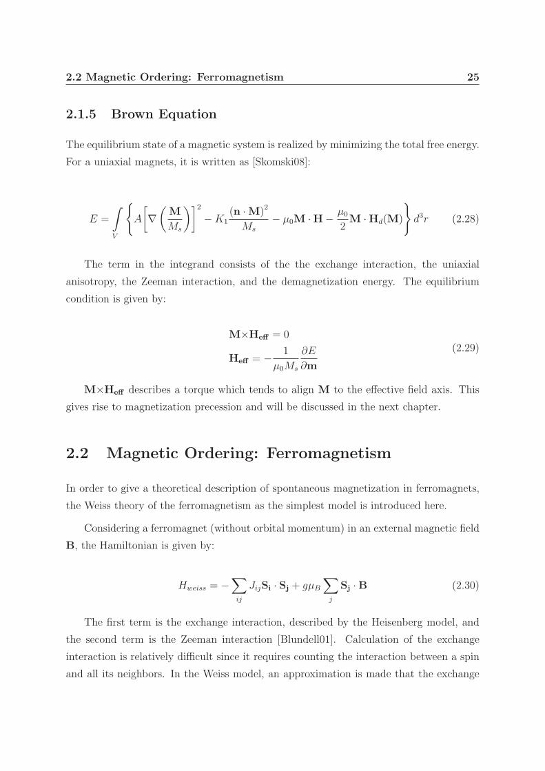
2.1.5 Brown Equation
The equilibrium state of a magnetic system is realized by minimizing the total free energy.
For a uniaxial magnets, it is written as [Skomski08]:
E =
∫V
{A
[∇
(M
Ms
)]2
− K1(n · M)2
Ms
− μ0M · H − μ0
2M · Hd(M)
}d3r (2.28)
The term in the integrand consists of the the exchange interaction, the uniaxial
anisotropy, the Zeeman interaction, and the demagnetization energy. The equilibrium
condition is given by:
M×Heff = 0
Heff = − 1
μ0Ms
∂E
∂m
(2.29)
M×Heff describes a torque which tends to align M to the effective field axis. This
gives rise to magnetization precession and will be discussed in the next chapter.
2.2 Magnetic Ordering: Ferromagnetism
In order to give a theoretical description of spontaneous magnetization in ferromagnets,
the Weiss theory of the ferromagnetism as the simplest model is introduced here.
Considering a ferromagnet (without orbital momentum) in an external magnetic field
B, the Hamiltonian is given by:
Hweiss = −∑ij
JijSi · Sj + gμB
∑j
Sj · B (2.30)
The first term is the exchange interaction, described by the Heisenberg model, and
the second term is the Zeeman interaction [Blundell01]. Calculation of the exchange
interaction is relatively difficult since it requires counting the interaction between a spin
and all its neighbors. In the Weiss model, an approximation is made that the exchange
2.2 Magnetic Ordering: Ferromagnetism 26
interaction is simplified by an effective molecular field Bmf , which is given by:
Bmf = − 2
gμB
∑j
JijSj (2.31)
This equation can be further simplified by taking Jij as a constant J for all neighbors
(the number is z) which gives the Bmf = 2zJS/gSμB.
The assumption is made that the molecular field is proportional to the magnetization:
Bmf = λM (2.32)
where λ is the molecular field constant, which is positive for ferromagnets.
The connection between the molecular field Bmf and the Curie temperature, Tc, can
be obtained from this model and is given by:
Tc =gSμB(S + 1)Bmf
3kB
(2.33)
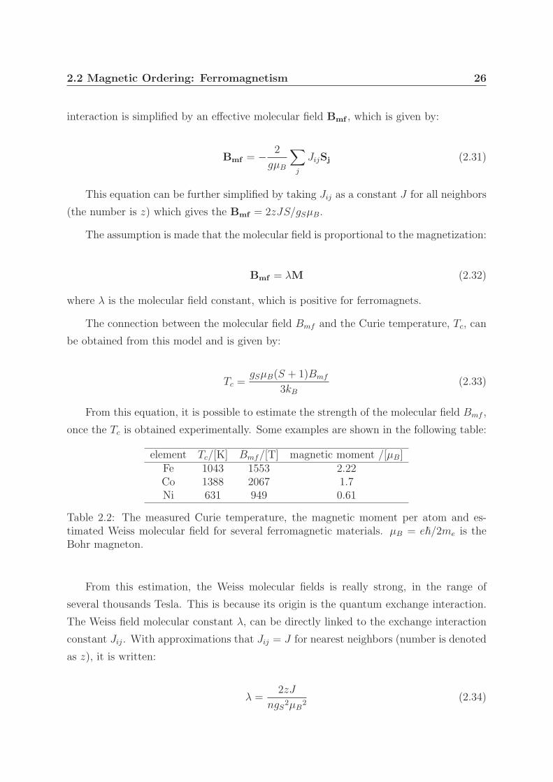
From this equation, it is possible to estimate the strength of the molecular field Bmf ,
once the Tc is obtained experimentally. Some examples are shown in the following table:
element Tc/[K] Bmf/[T] magnetic moment /[μB]Fe 1043 1553 2.22Co 1388 2067 1.7Ni 631 949 0.61
Table 2.2: The measured Curie temperature, the magnetic moment per atom and es-timated Weiss molecular field for several ferromagnetic materials. μB = e�/2me is theBohr magneton.
From this estimation, the Weiss molecular fields is really strong, in the range of
several thousands Tesla. This is because its origin is the quantum exchange interaction.
The Weiss field molecular constant λ, can be directly linked to the exchange interaction
constant Jij. With approximations that Jij = J for nearest neighbors (number is denoted
as z), it is written:
λ =2zJ
ngS2μB
2(2.34)
2.2 Magnetic Ordering: Ferromagnetism 27
The temperature dependent magnetization, M(T ), can also be obtained (for J = S =
1/2):
M(T )
M(0)= [3(1 − T
Tc
)]1/2 (2.35)
For other values of J , the magnetization as a function T, is plotted in Fig. 2.3
[Blundell01].
Figure 2.3: The magnetization of the Weiss model as a function of T, for different valuesof J .
From this, the conclusion is reached that in the Weiss model, the phase transition
between the ferromagnetic state and the non-magnetic state is a second order transition.
However, it is necessary to note that one of the major problems of the Weiss model
is that only the localized magnetic moments are considered, i.e., the Heisenberg model.
For 3d transition metals, Fe, Ni and Co, the conduction electrons, also called itinerant
electrons, are delocalized and hence can travel freely to any location in the sample. As
shown in table 2.2, the magnetic moment for Fe is 2.22 μB per atom and for Co is 1.7 μB.
Since each spin has a moment of 1 μB, these non-integer magnetic moments suggest that
the delocalized electrons have contribution to the total magnetization. For this reason,
the electronic band structure should be considered.
2.2 Magnetic Ordering: Ferromagnetism 28
A simple picture is that for the ferromagnets, due to the interaction between the free
electrons and the strong Weiss molecular field, the spins of some electrons around the
Fermi surface is flipped in order to achieve a lower system energy, i.e., to reach a stable
state of the electron distribution. This gives rise to a spontaneous magnetization without
the presence of an external magnetic field, given by M = μB(nup − ndown). This process
is only possible if the energy cost to flip the spin is smaller than the energy reduction
caused by interaction with the molecular field. This requirement is called Stoner criterion
and is given by:
Ug(EF ) � 1 (2.36)
where U = μ0μB2λ and it is proportional to the molecular field constant. Since λ
is a measure of the exchange energy, which is the result of the Coulomb interaction, as
shown in 2.2, U is therefore a measure of the Coulomb energy. The conclusion is that
the ferromagnetism is possible if the Coulomb interaction between free electrons is strong
enough and the number of electrons near the Fermi surface is large.
D(E ) D(E) D(E)
(a) (b) (c)
Figure 2.4: The density of states for bcc Fe, after [Skomski08]. (a), the initial paramag-netic state, (b) spin transfer caused by the exchange interaction and (c) the final state inwhich the density of states is distorted.
From 3d transition metals, there are two kinds of delocalized electrons: 4s and 3d
electrons. They both contribute to the electrical and thermal conductivities. But the
magnetic properties are mainly from the 3d electrons. The 4s electrons are almost free
from the nucleus, slightly deviated from the free electron model. Therefore they only
contribute to the Pauli paramagnetism. The spin transfer process is schematically shown
in Fig.2.4 [Skomski08]. In the initial state (a), the Stoner criterion is fulfilled by the large
density of states at the Fermi surface. The spin dependent energy splitting in the density
2.2 Magnetic Ordering: Ferromagnetism 29
of state for the 3d electrons occurs, as shown in (b). The Fermi surfaces for spin up and
spin down electrons are adjusted by shifting the density of states. The distortion of the
density of states is induced during this process, as shown in (c).
� � � � � � � � � �
� � � � � � � �
� � � � � � � �
� � � � � � � � �
� � � � � � � �
� � � � � � � � � �
� � � � � � � �
�
� � � � � � � �
� � � � � �
��
�� �
Figure 2.5: The Bethe-Slater-Neel curve [Kronmuller92]. The exchange energy is plottedas a function of the atomic disantce r0 (normalized to the radius of the 3d shell r3d.Exchange energy > 0 means ferromagnetism and < 0 means antiferromagnetism. Severalmagnetic materials are denoted on the curve.
As shown in Fig 2.4 (a), the density of the states near the Fermi surface is essential
to the formation of ferromagnetism. The atomic distance r0 makes a large influence on
the bandstructure and therefore it is one essential factor for the magnetic ordering. As
shown in Fig. 2.5, depending on the value of the r0, different types of magnetic ordering
can be formed:
• r0/r3d � 1, the repulsive force between the electrons is weak and this gives rise to
paramagnetism.
• r0/r3d � 1, the density of the states near the Fermi surface is small and the Stoner
criterion can not be realized. This leads to a state where the magnetic moments
are aligned antiparallelly.
• the value of r0 has a very small range where the magnetic moments are aligned
parallel. The stability of this configuration is realized by the energy reduction
caused by the large electron interaction with the Weiss molecular field.
Chapter 3
Magnetization dynamics
[Westphalen06]
3.1 Landau-Lifshitz-Gilbert Equation 31
“By studying nature,
man can overtake his imagination;
he can discover and understand
what he is even unable to imagine.”
– Lev Landau
In the previous chapter, the interactions and the corresponding energies inside a
magnetic system are described. The system achieves an equilibrium state by minimizing
the total free energy. However, the dynamic processes that the system experiences to
reach the equilibrium state is not discussed. Such knowledge is of great interest for
the magnetic data storage industry in order to achieve higher access speed, i.e., faster
magnetization reversal processes. In this chapter, the dynamic model proposed by Landau
and Lifshitz and later modified by Gilbert [Landau35] [Gilbert55] will be introduced.
3.1 Landau-Lifshitz-Gilbert Equation
In quantum mechanics, the time evolution of a system can be described by the time-
dependent Schrodinger Equation:
i�∂ |Ψ〉∂t
= H |Ψ〉 . (3.1)
The simplest situation of the magnetization dynamics is a spin in in the external
field B. The observable S, is given by the commutator with the Hamiltonian operator H
[Miltat02]:
i�∂S
∂t= [S, H] (3.2)
where the Hamiltonian is (Zeeman interaction) [Cohen87]:
H = −gμB
�S · B (3.3)
g = 2.002319304386 is the Lande g-factor. The z component of the commutator can
3.1 Landau-Lifshitz-Gilbert Equation 32
be expressed as:
[Sz, H] = igμB(S × B)x. (3.4)
The following expression can be summarized by deriving the same expression for the
other two components:
d
dt〈S〉 =
gμB
�(S × B). (3.5)
which is the time-dependent Schrodinger equation of a single spin in the magnetic
field. Considering a magnetic sample with homogeneous magnetization M, the system
can be described by a macrospin given by:
〈S〉 =�
gμB
M. (3.6)
Therefore, the equation of motion for the magnetization is described by a macrospin
model:d
dtM =
gμB
�(M × B). (3.7)
This equation is known as the Landau-Lifshitz equation and is normally expressed
as:d
dtM = γμ0M × H (3.8)
where γ = gμB/� < 0 is the gyromagnetic ratio. The γ0 = −γμ0 > 0 is introduced to
simplify the equation:d
dtM = −γ0M × H. (3.9)
A time-independent magnetic field leads to:
d
dt[M(t)]2 = 0
d
dt[M(t) · H] = 0
(3.10)
The first equation means during the motion around a constant external magnetic field,
the absolute value of the magnetization stays constant. The second equation expresses
that the angle between the magnetization and the external field does not change, as
3.1 Landau-Lifshitz-Gilbert Equation 33
shown in Fig.3.1 (a). The angular frequency is given by:
ω0 = γ0H (3.11)
which is proportional to the magnetic field (about 28 GHz/T ).
Figure 3.1: Magnetization precession without damping, (a), and with damping, (b)[Djordjevic06].
3.1.1 Damping
The conclusion is that, if the magnetization is excited out of the equilibrium, it takes
infinite time to relax. This is against the experimental observation since the equilibrium
state is always reached after a certain time. The reason is that the energy dissipation
during the motion is not considered. An ohmic type damping was proposed by Gilbert
and is given as:
α
Ms
(M × d
dtM) (3.12)
where α is the dimensionless and phenomenological Gilbert damping parameter. It
is a measure of the energy dissipation speed from the magnetization precession to the
magnetic system. By inserting this term into the equation, the Landau-Lifshitz-Gilbert
3.1 Landau-Lifshitz-Gilbert Equation 34
equation (the Landau-Lifshitz form) is introduced:
d
dtM = −γ0M × H︸ ︷︷ ︸
precessional term
+α
Ms
(M × d
dtM)︸ ︷︷ ︸
damping term
(3.13)
.
With the energy dissipation, the magnetization will precess around the external mag-
netic field with a gradually decreasing angle and finally it will be aligned to the axis of
the field, as schematically illustrated in Fig. 3.1 (b). This equation can also be written
differently by summing up the derivatives (the Gilbert form) [Brown63]:
dM
dt= − γ0
(1 + α2)M × H − αγ0
Ms(1 + α2)[M × (M × H)] (3.14)
One point worth noting here is that the phenomenological damping parameter α is
introduced to describe the energy dissipation. However, the exact underlying mechanisms
are still missing. The energy dissipation process is very complicated, which is one of the
reasons why research of magnetization dynamics is an active field. A brief review of several
important mechanisms for ferromagnets are introduced here. A more detailed summery
can be found in the following references [Djordjevic06], [Brown63] and [Miltat02].
The energy dissipation can be generally categorized into two types, depending on the
underlying mechanisms: the intrinsic and the extrinsic damping. The energy dissipations
caused by electron phonon scattering or electron magnon scattering are called intrinsic,
because they are an integral part of the magnetic system and are inevitable. However, the
contributions from geometrical effects, structural defects and non-uniform excitation can
be avoided and are called extrinsic [Heinrich05]. Experimentally, the intrinsic damping
of the system is considered to be the the smallest measured damping under well defined
conditions.
Intrinsic Damping
Kambersky was one of the pioneers to study the origin of the damping parameter in the
1970s [Kambersky70]. It was experimentally observed that the Fermi surface is changed
during the magnetization precession. This is because in ferromagnets, the magnetization
is mainly from the spins and therefore during the magnetization precession, the spins are
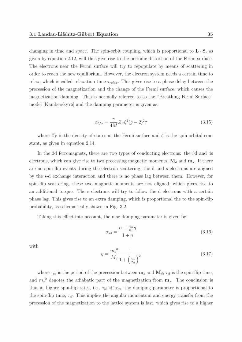
3.1 Landau-Lifshitz-Gilbert Equation 35
changing in time and space. The spin-orbit coupling, which is proportional to L · S, as
given by equation 2.12, will thus give rise to the periodic distortion of the Fermi surface.
The electrons near the Fermi surface will try to repopulate by means of scattering in
order to reach the new equilibrium. However, the electron system needs a certain time to
relax, which is called relaxation time τrelax. This gives rise to a phase delay between the
precession of the magnetization and the change of the Fermi surface, which causes the
magnetization damping. This is normally referred to as the “Breathing Fermi Surface”
model [Kambersky76] and the damping parameter is given as:
αbfs =γ
4MZF ζ2(g − 2)2τ (3.15)
where ZF is the density of states at the Fermi surface and ζ is the spin-orbital con-
stant, as given in equation 2.14.
In the 3d ferromagnets, there are two types of conducting electrons: the 3d and 4s
electrons, which can give rise to two precessing magnetic moments, Md and ms. If there
are no spin-flip events during the electron scattering, the d and s electrons are aligned
by the s-d exchange interaction and there is no phase lag between them. However, for
spin-flip scattering, these two magnetic moments are not aligned, which gives rise to
an additional torque. The s electrons will try to follow the d electrons with a certain
phase lag. This gives rise to an extra damping, which is proportional the to the spin-flip
probability, as schematically shown in Fig. 3.2.
Taking this effect into account, the new damping parameter is given by:
αsd =α + τex
τsfη
1 + η(3.16)
with
η =ms
0
Md
1
1 +(
τexτsf
)2 (3.17)
where τex is the period of the precession between ms and Md, τsf is the spin-flip time,
and ms0 denotes the adiabatic part of the magnetization from ms. The conclusion is
that at higher spin-flip rates, i.e., τsf � τex, the damping parameter is proportional to
the spin-flip time, τsf. This implies the angular momentum and energy transfer from the
precession of the magnetization to the lattice system is fast, which gives rise to a higher
3.1 Landau-Lifshitz-Gilbert Equation 36
Figure 3.2: Intrinsic damping induced by the exchange interaction between s and delectrons, after [Djordjevic06]. Without spin-flip scattering, no extra damping is induced(left). If the spin-flip occurs, extra torque is induced to push ms toward Md and thiscauses an additional damping term.
damping parameter [Djordjevic06].
The eddy currents, caused by the magnetization precession, can also contribute to
the magnetic damping. The effective damping parameter is given by:
αeddy =(Msγ)2
6
4π
c2σd2 (3.18)
where σ is the electrical conductivity and d is the film thickness. Since this damping
term deceases dramatically when reducing d, it can be neglected for thin films. It was
estimated that for permalloy, the effect of eddy currents is insignificant when d < 100 nm
[Heinrich05].
The direct magnon-phonon scattering is another damping mechanism, for which the
damping parameter is written as:
αph = 2ηγ2
(B2(1 + ν)
E
)2
(3.19)
where η denotes the velocity of the phonon, B2 is the magnetoelastic shear constant,
E is the Young’s modulus and ν is the Poisson ratio [Heinrich05]. However, this effect
was estimated to be very small for metallic ferromagnets [Woltersdorf04] and hence is
3.1 Landau-Lifshitz-Gilbert Equation 37
also neglected.
Extrinsic Damping
The structural defects or inhomogeneities can give rise to magnetization damping, re-
ferred to as extrinsic damping [Heinrich05]. The main contribution to this damping is
the two-magnon scattering process, in which a uniform precession scatters to nonuniform
modes (magnons). The energy is therefore transferred from the uniform magnetization
precession into the nonuniform modes, however the total magnetization energy is con-
served. The intrinsic damping between the nonuniform modes and the lattice system will
give rise to the energy dissipation. Another possible damping mechanism, referred to as
the radiation damping mechanism, has been proposed for time-resolved MOKE experi-
ments. The spin waves with finite wavelength are excited locally (inside the laser focus)
and propagate into the unexcited region of the sample (outside the focus). This energy
transfer will cause an additional damping and it was estimated experimentally that this
process can lead to a 25 % increase of the damping parameter in 10 nm permalloy films
[Jozsa05].
3.1.2 Uniform Precession
The precessional angular frequency of a macrospin in the external field is given in equation
3.11. By replacing the external field with the effective field, derived from equation 2.29,
all contributions of the anisotropy, the exchange interaction, and the external field are
included:
d
dtM = −γ0M × Heff (3.20)
where
Heff = − 1
μ0Ms
∂E
∂m. (3.21)
From this, the angular frequency can be derived in a spherical coordinate system as
a function of the free energy [Djordjevic06]:
ω =γ0/μ0
Ms sin θ
ö2E
∂θ2
∂2E
∂ϕ2−
(∂2E
∂θ∂ϕ
)2
(3.22)
3.1 Landau-Lifshitz-Gilbert Equation 38
where θ and ϕ are the normal and polar angles, respectively. This is a general formula
and approximations are needed to simplify it. For a thin film, if the shape anisotropy, the
intrinsic uniaxial anisotropy and the external field are considered, the angular frequency
of the magnetization precession can be calculated as [Djordjevic06]:
ω =γ0/μ0
sin θ·√(
−2Kx
Ms
+2Kz
Ms
− μ0Ms
)cos 2θ + μ0Hx sin θ + μ0Hz cos θ (3.23)
·√(
2Kx
Ms
− 2Ky
Ms
)sin2θ + μ0Hx sin θ (3.24)
This describes a uniform (coherent) precessional motion for all magnetic moments
and is called the Kittel model.
3.1.3 Spin Waves
A single macrospin is surely not enough to describe the magnetization dynamics of a whole
system. The first deviation from this model is the non-uniform precessional motions, i.e.,
the magnetic moments have the same angular frequency but with a different phase. This
is schematically shown in the Fig. 3.3.
Figure 3.3: Schematic illustration of spin waves in one-dimensional spin system, after[Michael06]. a) The Kittel mode, i.e., k = 0. b) The higher order modes with k �= 0.
To describe the spin wave mathematically, the wave vector k is defined as |k| = 2π/λ
3.1 Landau-Lifshitz-Gilbert Equation 39
with λ as the wavelength. Depending on the length scale, spin waves can be generally
categorized into two types: if the wavelength is much shorter than the exchange length
scale Λ, exchange interaction dominates and this is referred to as “spin waves”; if the
wavelength is large, the magnetic dipolar interaction can be dominating and it is called
as “magneto-static waves”.
There are many approaches to calculate the dispersion relation for the spin waves. The
readers are suggested to find more details about this subject in the reference [Stancil93]
[Demokritov02] [Demokritov09] [Djordjevic06]. The Herring-Kittel formula, which in-
cludes the exchange interaction for infinite ferromagnets, is introduced for this purpose:
ω = γμ0
√(H +
2k2A
μ0Ms
) (H + Mssin
2θk +2k2A
μ0Ms
)(3.25)
where θk denotes the angle between the wave vector k and the magnetization M.
As concluded in the reference [Eilers06], in an all-optical pump-and-probe experiment,
the spin waves propagating in the lateral direction in thin films are not important on
the time scale of ns. The perpendicular standing spin waves (PSSW) can be observed
experimentally. This type of spin wave mode is schematically shown in the Fig. 3.4
Figure 3.4: Fixed boundary conditions for the PSSW modes in a thin film. The directionof the magnetization is in plane and hence vertical to the wave vector k.
3.2 Laser induced magnetization dynamics 40
3.2 Laser induced magnetization dynamics
Magnetization dynamics has been discussed in the previous section, but the experimental
approaches to induce it in the magnetic system was not included. As shown in the
Fig. 1.7, there are mainly three methods to excite the magnetic system and initiate
the dynamics. Excitations using a magnetic field pulses H(t) are the easiest case for
theoretical treatment since only the spin systems are perturbed. Thermal excitation T (t)
with intense laser pulses, which is used in this thesis, induced very different dynamics
because all three systems, namely the electron, the spin and the phonon systems, are
excited and hence additional description which includes the dynamics of the three systems
and the interaction between them are necessary.
Figure 3.5: Remanent longitudinal MOKE signal of 20 nm Ni film after laser excitation.
The first attempt to excite the ferromagnets using pulsed laser system was done by
Agranat [Agranat84]. Laser pulses with various duration (from few ps to 40 ns) was
used to excite the Ni thin film. Their conclusion was that heat-induced demagnetization
process occurs on a ns time scale. Few years later, Vaterlaus used time-resolved spin-
polarized photoemission technique with 10 ns pump duration and 60 ps probe duration
to study magnetization dynamics on Gd film. The result demonstrated a spin relaxation
time of 100±80 ps [Vaterlaus91]. Huebner et al. has estimated a spin relaxation time of
48 ps, which attributes to the time scale of spin-lattice interaction [Huebner96]. These
early studies lead to a generally accepted conclusion that laser-induced demagnetization
occurs on the time scale of 100 ps and is attributed to the spin-lattice interaction.
3.2 Laser induced magnetization dynamics 41
The experiment done by Beaurepaire et al. gave a astonishing result: they observed a
demagnetization on a picosecond time scale. A pump-and-probe MOKE technique with
pulse duration of 60 fs was used. They observed the remanent MOKE signal decreased
after the optical excitation and reached the minimal at 2 ps, as shown in Fig. 3.5. Their
conclusion was that the ultrafast demagnetization was attributed to the electron-spin
scattering process. This work triggered a new development in the field of magnetization
dynamics. However, Koopmans et al. have carried out similar experiments but they
recorded both Kerr rotation and ellipticity at the same time [Koopmans00]. By comparing
the two signals, they have identified nonmagnetic contribution to the magneto-optical
response and the conclusion was that the drop in the MOKE signal was due to the optical
artifacts caused by the dichroic bleaching effect. On the contrary, from the experimental
data obtained on CoPt3 system, it is confirmed that the fast drop of MOKE signal within
the first 100 fs does represent the magnetization dynamics [Bigot04]. The explanation
was the fast spin dynamics occurs on the 50 fs time scale during the thermalization of
the electron system.
���� ��� ��� ��� ��� �
�
�
�
��
��
��
��
���
�������
�������
��������
��������
��������
��������������������
!��"�
��"!
�#$
%&
���'
"����
����
��"�
!�
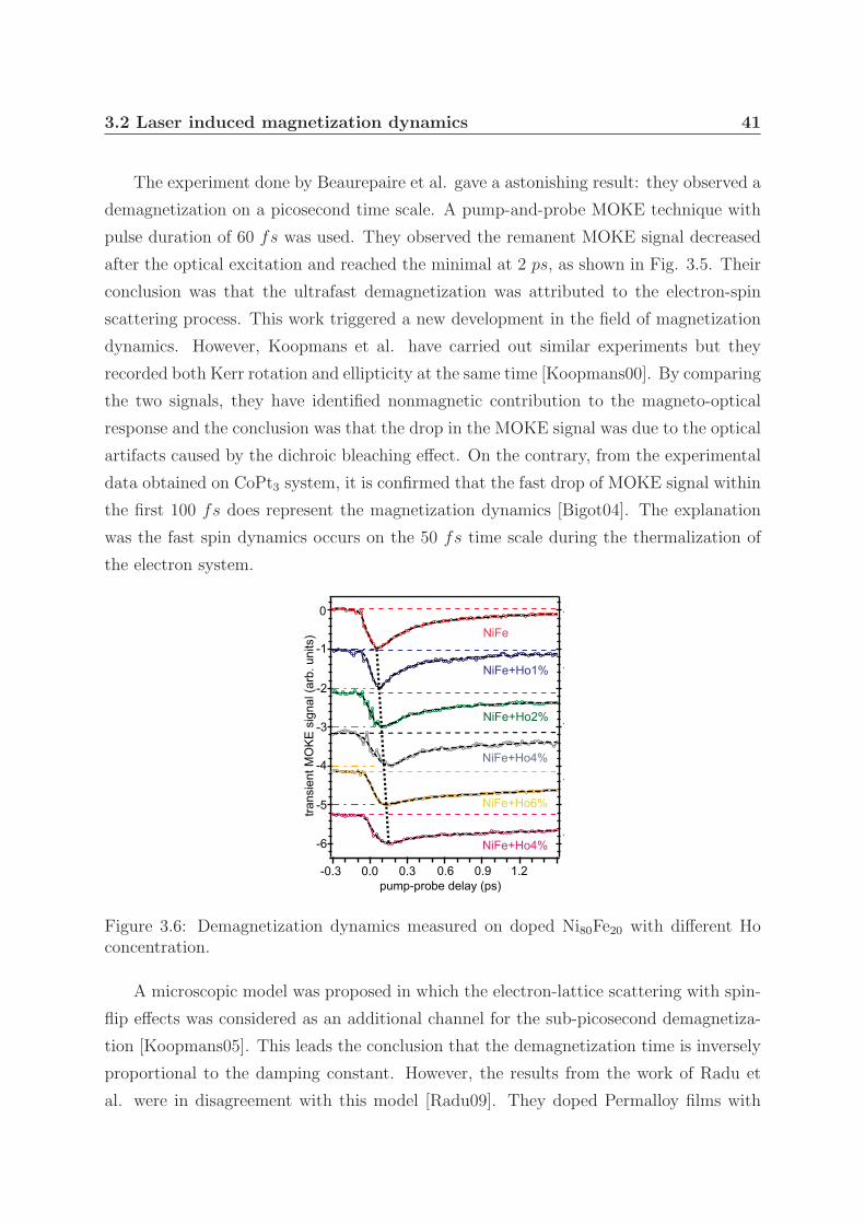
Figure 3.6: Demagnetization dynamics measured on doped Ni80Fe20 with different Hoconcentration.
A microscopic model was proposed in which the electron-lattice scattering with spin-
flip effects was considered as an additional channel for the sub-picosecond demagnetiza-
tion [Koopmans05]. This leads the conclusion that the demagnetization time is inversely
proportional to the damping constant. However, the results from the work of Radu et
al. were in disagreement with this model [Radu09]. They doped Permalloy films with
3.2 Laser induced magnetization dynamics 42
Ho, Dy and Tb at different concentration and observed a gradual increase of the demag-
netization time from 60 to 150 fs, as shown in Fig. 3.6. This leads to the argument
that Koopmans’ description of the demagnetization dynamics based on impurity-assisted
spin-flip scattering process gives a rather over simplified view for 4f impurities.
Bigot’s recent study [Bigot09] has shown the 50 fs laser pulse is coupled to the spin
systems in a ferromagnetic metals during its own propagation. It is suggested that the
photon field induces polarization, which interacts with the spins and causes the demag-
netization process on sub ps time scale. In this process, the dynamics has its origin in
relativistic quantum electrodynamics.
In a recent work by C. La-O-Vorakiat et al., femtosecond soft x-ray pulses were
used to obtain element-specific demagnetization dynamics of FeNi system [Vorakiat09].
However, due to the strong exchange interaction, they did not see a significant difference
in the demagnetization dynamics between Fe and Ni. Nonetheless, this approach opens
the possibility to detect magnetization dynamics on the femtosecond time scale with
nanometer spatial resolution and element specificity.
3.2.1 Two Temperature Model: e-l interaction
When the pump laser pulse arrives at the sample, the electrons are thermally excited by
absorbing the photons. This process is governed by the Lambert-Beer’s law (by neglecting
the multiple reflections and scattering):
I(d) = I0e−α(ω)d (3.26)
where α is the optical absorption coefficient. It is clear that the light is absorbed
non-uniformly at different depth and the the optical penetration depth is defined as:
δ =λ
4πk=
1
α(3.27)
where k is the imaginary part of the refractive index and λ is the wavelength of the
light. For metals, δ is in the range of 10 to 30 nm. Less than 10 fs after the optical
excitation, phase coherence between the excited electrons is destroyed by the electron-
electron, electron-thermal phonon or electron-defect scattering. The kinetic energy of the
3.2 Laser induced magnetization dynamics 43
electrons remains unchanged on this time scale. This process gives rise to the randomized
momentums of the electrons and this schematically illustrated in the top part of Fig. 3.7
[Radu06].
Figure 3.7: Transient electron dynamics induced by laser pulses, after [Radu06]. At t = 0,few electrons near the Fermi surface are excited by absorbing the photons with energyhν and non-Fermi distribution of the electron density is formed. After a certain time τth,which is in the order of few 100fs, the electron system reaches a new equilibrium statethrough electron-electron scattering. Finally, the energy is transferred from electronsystem to the phonon system and the new equilibrium state for the whole system isrealized.
Although the phase coherence of the hot electrons are destructed, the electron system
still remains in a highly non-equilibrium state because energy redistribution does not
occur in the first step. The following electronic thermalization process through inelastic
electron-electron scattering will bring the electron system back to equilibrium, as shown
in the middle part of Fig. 3.7.
Generally speaking, there are two kinds of electron-electron scattering processes: at
3.2 Laser induced magnetization dynamics 44
low excitation density (< 10−3e−/atom), one hot electron scatters with the unexcited
electron at the Fermi surface. However, once the excitation density is above the threshold,
scattering process can occur between hot electrons and the hot electron system will reach
its own equilibrium first and then scatters with unexcited electron bath.
The life time of the hot electrons at low excitation density can be derived from the
Landau’s Fermi-liquid theory (FLT) [Quinn62] and is given by (at T = 0):
τe−e = τ01
(E − EF )2 (3.28)
where τ0 ∝ n5/6 and n is the electron gas density. At finite temperature, this formula
is changed to [Quinn62]:
τe−e =1
2β[(πkBT )2 + (E − EF )2] (3.29)
where β is the electron-electron scattering probability.
For all-optical pump-and-probe experiments, the excitation density is normally high
enough to give rise to scattering between hot electrons. A equilibrium temperature Te
is firstly reached for excited electrons before significant energy transfer to the unexcited
electrons. Due to the small heat capacity of the electron systems, Te can be a few 1000
K.
After the thermalization of the electron system, there is still a temperature difference
between the electron and the lattice systems. Energy transfer will occur in the next
few picoseconds and finally the whole system reaches its own equilibrium with a slightly
higher temperature. The electron-phonon interaction can be considered as local distortion
of the lattice caused by the phonon and then in turn change the local electronic structure.
The time scale of this interaction can be estimated by the Debye model and is given by
[Grimvall81]:
τe−l =2πλkBT
�(3.30)
where λ is the e-p mass enhancement factor which describes the e-p interaction
strength. kB is Boltzmann constant.
In addition to the energy transfer, electron diffusion process will also cause the en-
3.2 Laser induced magnetization dynamics 45
ergy redistribution. This is caused by the local excitation and the non-uniform photon
absorption in the vertical direction. The two temperature model (2TM) was proposed
by Anisimov [Anisimov74] to describe the energy redistribution in time and space. The
assumption is that the electron and lattice system are in a local thermal equilibrium and
two equations are used to describe the energy transfer between them:
Ce(Te)δTe
δt=
δ
δz
(Ke
δTe
δz
)− gel (Te − Tl) + S(z, t)
ClδTl
δt= gel (Te − Tl)
(3.31)
where Ce = γTe with γ as a constant determined by the density of state at Fermi surface.
Cl is the heat capacity of the lattice system. Ke is the electronic thermal conductivity and
gel is the coupling constant between electron and lattice system. The optical property of
the system is described by the term S(z, t), which is given by:
S(z, t) = (1 − R − T )I0αe−( tτ)2
(3.32)
where R and T are the reflectance and transmittance of the system and τ is the laser
pulse duration.
After excited area reaches the localized thermal equilibrium, temperature gradient
in the system will give rise to the thermal diffusion from the excited hot area to the
unexcited part of the sample. Then system relaxes to the final equilibrium state.
3.2.2 Three Temperature Model: s-e-l interaction
So far, the spin system is neglected during the relaxation. An additional term, which
describes the spin system, is added to the two temperature model and this is normally
referred to as the three temperature model (3TM). In this case, the spin temperature is
defined from the M-T-diagram, as shown in Fig. 3.8.
As firstly proposed by Vaterlaus et al. [Vaterlaus92], the spin system is simply de-
scribed by a single spin temperature Ts, which is very rough approximation, but works
well in many situations [Koopmans03]. The partial differential equations for 2TM is thus
3.2 Laser induced magnetization dynamics 46
Figure 3.8: A typical M-T diagram for ferromagnets and the effect of laser heating,after [Koopmans03]. The absorption of the photon energy causes a temperature increaseΔT = T2 − T1 and a magnetization decrease of ΔM .
modified as the following:
Ce(Te)δTe
δt= ∇Ke∇Te − gel (Te − Tl) + S(r, t)
Cl(Tl)δTl
δt= gel (Te − Tl) + gls (Ts − Tl)
Cs(Ts)δTs
δt= ges (Te − Ts) + gls (Tl − Ts)
(3.33)
with ges and gls are the coupling constant between the electron, spin and lattice
system. Cs is the heat capacity of the spin system. An example of this model is the
work of Beaurepaire on ferromagnetic polycrystalline Ni samples with thickness of 22 nm
[Beaurepaire96]. The calculated temperatures for electron, spin and lattice systems are
plotted in Fig. 3.9. It is concluded that within 2 ps, the spin temperature Ts was increase
to 575 K for pulses of 7 mJcm−2. The thermal conductivity is neglected on the time
scale of ps, i.e., Ke = 0, which is generally correct for thin films.
The interaction in the heat bath which includes electron, spin and lattice system is
schematically illustrated in the Fig. 3.10 [Koopmans03].
3.3 Magneto-optical Kerr Effect 47
Figure 3.9: The estimated electron, spin and lattice temperature of the Ni film using thethree temperature model [Beaurepaire96].
electrons
(T )e
spins(T )s
lattice(T )l
ges
gel gsl
laserS(r,t)
Figure 3.10: Schematic illustration of the energy transfer in the 3TM. Note that onlythe electron system is excited by the laser pulse which gives rise to a increase of Te. Thefollowing energy transfer takes place on different time scales.
3.3 Magneto-optical Kerr Effect
So far, a general description of magnetization dynamics is given. Some special mechanisms
triggered by intense laser pulse is also discussed in the previous sections. This is thesis,
the magnetization dynamics induced by the pump laser pulse is detected by the probe
pump in the polar MOKE geometry. It is therefore necessary to give a description of the
magneto-optical Kerr effect.
As discovered by John Kerr in 1876 [Kerr76], the magneto-optic Kerr effect (MOKE)
has been one of the most useful tool for the magnetism research community [Hubert00].
There are three configurations for the Kerr effect experiments categorized by the relative
3.3 Magneto-optical Kerr Effect 48
Longitudinal Polar Transversal
MM M
(a) (b) (c)
Figure 3.11: Schematic illustration of three types of Kerr effect: (a) longitudinal, (b)polar, and transversal (c), after [Kleeman07].
orientation between the light to the magnetization and the sample plane, as shown in
Fig. 3.11.
Generally speaking, MOKE causes two types of changes in the polarization state
of the incident light (linearly polarized): after reflected by the magnetic sample, the
polarization plane is rotated by an angle, which is referred to as the Kerr rotation angle
θk and the an ellipticity is added, which is called Kerr ellipticity εk. A classic picture
of this effect is that the Lorentz force affects the motion of the electrons excited by the
incident electromagnetic wave. Despite the simplicity, this explanation does not account
for the reality because it requires magnetic fields in the order of 104 tesla to cause the
amplitude of the MOKE signal observed experimentally.
In a phenomenological approach, the dielectric tensor of the optical isotropic material
is given by:
ε(ω) =
⎛⎜⎜⎝
εxx 0 0
0 εyy 0
0 0 εzz
⎞⎟⎟⎠ (3.34)
With magnetization M, the sample becomes optically anisotropic. The off-diagonal
3.3 Magneto-optical Kerr Effect 49
elements of the dielectric tensor decries the effects of the magnetization:
ε(ω) =
⎛⎜⎜⎝
εxx εxy −εxz
−εxy εyy εyz
εxz −εyz εzz
⎞⎟⎟⎠ (3.35)
Note that the time-reveral symmetry is broken with magnetization:
εij(M) = −εij(−M) (3.36)
Expanding εij in powers of M, one obtains:
εij(M) = εij(0) +δεij
δMM (3.37)
This leads to the conclusion that the diagonal elements are independent from the magne-
tization and the off-diagonal elements are related to the component of M that is parallel
to i × j.
To give a simple picture, the Kerr effect scenario is considered as the following: a
linearly polarized incident light is decomposed to left and right hand circularly polarized
light with equal intensity. The different refractive indexes these two parts experience
give rise to a phase shift. This causes the Kerr rotation. The different absorption rate
gives rise to the amplitude difference between the left and right hand circularly polarized
modes, which leads to the Kerr ellipticity. For the polar MOKE geometry, the complex
Kerr angle is given as [Radu06]:
Θk = θk + iεk ∼ εxy
εxx
∼ M (3.38)
From this equation, one easily derives the following relation [Koopmans03]:
Δθ(t)
θ(t = 0)=
Δε(t)
ε(t = 0)=
ΔM(t)
M(t = 0)(3.39)
However, this explanation is only phenomenological. The microscopic origin of the
off-diagonal elements is connected to the spin-orbit coupling. With the independent
electron approximation, the dielectric tensor and the electronic structure are related as
3.3 Magneto-optical Kerr Effect 50
the following [Koopmans03]:
εij(ω) = δij +4e2
π�m2ω2
∑gn
∫BZ
dk3ωgn,k[fg,k(1 − fn,k)]
(|P+
gn|2±ij|P−gn|2
)ω2
gn,k − ω2 − 2iωΓgn,k
(3.40)
where ij equals xx or xy. The operator ±ij is + for ij = xx and − for ij = xy. g and
n are Bloch states indexes, indicated by the wave vector k and fn,k is the occupation
percentage of the corresponding state. The energy different between bands g and n at
wave vector k is denoted as �ωgn,k and �Γgn,k is the lifetime broadening of this transition.
The quantity P±gn,k is defined as:
P±gn,k = 〈Ψg,k| − i�(∇x ± i∇y) |Ψn,k〉 (3.41)
It is important to note that for 3d transition metals, the orbital momentum is largely
quenched by the crystal field effects. Therefore, the spin momentum gives main contri-
bution to the magnetization and orbital momentum gives a very small contribution. The
Kerr effect only probes the orbital momentum, which is a small fraction of the total mag-
netic moment. One has to assume that a fixed ratio of the orbital and spin components
of M to predict the total magnetic moment from the Kerr effect. In addition, as shown
by Koopmans [Koopmans05] and Oppeneer [Oppeneer04], for the laser excitation experi-
ments the optical dielectric tensor is modified by the non-equilibrium electron distribution
right after the high intensity laser excitation. This gives rise to the disproportionately
between the Kerr rotation and the ellipticity. Therefore, the Kerr response with in the
first ps constants both magnetization information and non-magnetic optical artifact.
Chapter 4
Time-resolved Scanning Kerr
Microscope
52
“It doesn’t matter how beautiful your theory is,
it doesn’t matter how smart you are.
If it doesn’t agree with experiment, it’s wrong”
– Richard Feynman
The main part of the work for this thesis is the designing, installation and testing of
a time-resolved scanning Kerr microscope. The whole setup is show in the Fig. 4.1. A
detailed description of the design of the mechanical components, such as the hatch, the
holders and optical table, can be found in the master thesis of Bjorn Redeker [Bjoeorn08].
In this chapter, a introduction of the key optical and mechanical components and the
controlling software is included.
The equipments used in the setup together with the controlling software are discussed
in this part of the thesis. First, the light source of the microscope, the Ti:sapphire
oscillator, and the frequency-doubling crystal is described, following is the techniques to
reach temporal and spatial resolutions. The signal detection and processing is discussed
in the last section.
delaystage
GDD mirrorcompressor
polarizersample
magnet
chopper
analyzer
PEM
detectors
prism1 for GDDcompensation
prism 2 for GDDcompensation
BBOcrystal
3D piezoscanning stage
Zeiss100 /0.95x
microscopeobjective
chopper
�/2 plate
Scie
ntific
XL
FE
MT
OL
AS
ER
S
Figure 4.1: Scheme of the time-resolved scanning Kerr microscope.
4.1 Light Sources 53
4.1 Light Sources
The temporal-resolving ability of this microscope is realized by means of all-optical pump
and probe technique, in which two laser beams are needed. Most of the TR-MOKE
setups use a pump and a probe beam generated by splitting the fundamental output of
a femtosecond laser using a beam-splitter. Such a single color design means lower cost
and easier operation. However, there are several problems that full attention needs to be
paid. Since the pump and probe beam has the same wavelength, after reflected from the
sample surface, it is difficult to separate the probe beam, which carries magnetic signal at
much lower power, from the scattered high-power pump beam. Because the modulated
MOKE signal is only a small change of the output voltage from the detector, even a slight
fraction of the pump beam will make large disturbance on the signal. Also, the longer
wavelength, typically from 760 to 800 nm, limits the spatial resolution of the setup.
To overcome these limits, a two-color pump and probe configuration is used, i.e., the
fundamental beam from the oscillator pumps the system and the frequency-doubled beam
probes the change of the magnetization. Since their wavelengths are very different (780
nm and 390 nm), the probe beam is therefore easily separated from the scattered pump
beam by folding the beams several times between two mirrors with high reflection ratio
for the probe beam and high transmission ratio for the pump beam. In addition, a half-
wave plate has been placed into the path of the pump beam, which makes the polarization
perpendicular to the optical table, i.e., s-polarized. However, the photoelastic modulator
(PEM) is mounted on the holder with its optical axis parallel to the table so that only the
p-polarized probe beam is modulated at 50 kHz. Since the pump beam is s-polarized, it
is nearly not modulated and hence the disturbance is further reduced. This two levels,
i.e., wavelength and polarization, filtering configuration enables the detection of MOKE
signal nearly free of pump disturbance. The detailed description of signal detection and
noise filtering is included in the section 4.4 of this chapter.
4.1.1 Ti:sapphire Oscillator
To study a phenomenon that is fast, one needs a detection technique that is even faster.
The solid-state pulsed laser is nearly a universal experimental device to study processes
which occur in the picosecond or nanosecond regime. To generate a laser pulse with
a duration of femtoseconds, a mode-locking technique is commonly used. The physical
4.1 Light Sources 54
principle of this technique is to induce a fixed phase relationship between the different
longitudinal modes of the laser’s resonant cavity. A series of short pulses are gener-
ated by the interference between these longitudinal modes, as explained in the book of
Chang [Chang05]. The shortest directly-generated pulses are produced by mode-locked
Ti:sapphire lasers with a duration of about 5 fs [EllR01]. It has been demonstrated that
one can reach a pulse duration shorter than 100 as (attoseconds) using high harmonic
generation with amplified laser systems [Baltuska05] [Goulielmakis05]. The radiation is
in the soft x-ray regime and thus not suitable for MOKE. However x-ray magnetic cir-
cular dichroism (XMCD) could once become an option for magnetic imaging and such a
system may provide element specific capability, sub-femtosecond temporal resolution and
high spatial resolution. Despite all these attractive advantages, an attosecond soft x-ray
system has not yet been demonstrated to study magnetization dynamics. The difficulties
might be the low intensity output and the technical challenges to produce high quality
optics for attosecond pulses with a wavelength in the soft x-ray regime. Nevertheless,
there are a few research groups trying to solve these challenges and it is likely that such
systems will be demonstrated in the foreseeable future. Currently, most of TR-MOKE
setups use commercially available mode-locked Ti:sapphire lasers, which normally give
output pulses with a duration below 100 fs.
In our experimental setup, a Ti:sapphire oscillator, “Scientific XL” from FEMTO-
LASERS Produktions GmbH, is pumped at 7 Watt by a diode-pumped solid-state Nd:YVO4
laser (Verdi-10 from Coherent), as shown in Fig. 4.2. Such an all-solid-state setup guar-
antees an outstanding stability (maximum pulse-to-pulse energy variations are well be-
low 3% and the standard deviation over 1000 pulses is less than 0.38%) [Fuerbach04]
[Fernandez04]. The emitted infrared radiation has a fixed central wavelength of 782 nm
with a spectral FWHM of more than 38 nm, which supports a pulse duration well below
60 fs. By means of multipass cell configuration, the length of the resonator is extended
up to 12.6 m, corresponding to a repetition rate of 11 MHz [Fuerbach04] [Fernandez04].
In comparison to typical oscillators, which have repetition rates between 70 and 90 MHz,
this type of oscillator gives two advantages for our all-optical pump and probe application:
firstly, the time interval between two successive pulses is increased up to 90 ns, meaning
that there is plenty of time for relaxation after optical excitation; secondly, the energy for
each pulse is raised to 80 nJ, which is enough of many thermal excitation experiments.
4.1 Light Sources 55
Verdi V10Pump Laser
8 bounces
Figure 4.2: The optical components inside the Ti:sapphire oscillator. Note that the beamis reflected 8 times between two telescope mirrors, which gives a total resonator lengthof 12.6 m [Fuerbach04].
4.1.2 Frequency-doubled Beam
The high output power of the oscillator, 860 mW and 1100 mW when pumped at 7.0
W and 8.0 W , respectively, is sufficient to generate a frequency-doubled probe beam. As
shown in Fig. 4.3, the fundamental beam from the oscillator is focused to the β-BaB2O4
(BBO) crystal using a lens with a focal length of 50 mm.
By fine-tuning the position of the BBO crystal with a 3D mechanical translation
stage, marked as (C), the power of the generated probe beam is maximized to 165 mW ,
i.e., the conversion efficiency is above 19 %. The pump and probe beams are separated
by a thin beam splitter, marked as D in Fig. 4.3, with a high transmittance at 800 nm
and high reflectance at 400 nm, and then collimated by two lenses, designated as (E) and
(F) in Fig. 4.3.
Since the pump and probe beam are now spatially separated, controlling the time
delay between both pulses is possible.
4.1 Light Sources 56
(A) (B)
(C)
(D)
(E)
(F)
BBO
Figure 4.3: The β-BaB2O4 (BBO) crystal , mounted in holder (B), generates the probebeam. The optical paths of both beams are marked by red and blue arrows.
4.2 Temporal Resolution 57
4.2 Temporal Resolution
In pump and probe experiments, the temporal resolution is realized by tuning the time
delay between the excitation and the detection. An electronic pulser, such as AVMR-A-
B from AVTECH electrosystems, is able to generate current pulses with a rise time of
150 ps and to control the delay time with respect to the triggering signal. The temporal
resolution is, however, restricted by the jitter, i.e., the peak-to-peak displacement between
two adjacent output current pulses, which is typically about few hundred ps for cost
effective pulsers and can be as low as 10 ps for high-performance pulsers. Such an simple
electronic solution provides easy operation and therefore it is widely used in many pump-
and-probe experiments as long as the temporal resolution is not limited by the pulse
jitter. However, at the current stage of technology development, varying the delay time
in the fs regime is still impossible just with electronics devices.
For optical pump-and-probe experiments, this limit can be circumvented by varying
the difference of the path between the pump and probe beam and hence control the
time they arrive at the sample surface. A motorized mechanical translation stage with a
moderate spatial accuracy is thus capable of reaching a temporal accuracy of less than
100 fs. The total temporal scanning range is limited by the traveling length of the stage,
but if one of the beams is folded two times by a mirror pair mounted on the stage, the
total delay time can be doubled.
4.2.1 Delay Stage
A direct drive linear motor stage, Lineax-10 from Nutec, as shown in Fig. 4.4, is used
in this setup to control the delay time. Compared to conventional screw driven stages,
such type of motor translation stages have many advantages such as faster settling, more
precise motion path and higher repeatability. The high precision version of Lineax-10
has been selected providing a relative positional accuracy of less than 0.5 μm over 25
mm traveling range, which corresponds to a relative temporal accuracy of less than 1.6
fs. The total traveling length is 1.2 m, which means by folding the beam once with one
mirror pair, a total temporal scanning range of 8 ns can be realized. In case a larger
temporal range is required, e.g., for the processes that have low damping factors and
hence take longer time to relax, the beam can be folded twice by installing one more
mirror pair additionally. This will result in a large temporal range of 16 nm.
4.2 Temporal Resolution 58
Figure 4.4: The translation stage for tuning the temporal spacing between pump andprobe beam. (A), the track of the stage; (B) the moving plate on which the mirror pair,marked as (C), is mounted.
4.2 Temporal Resolution 59
One of the most crucial problems of this technique is the existence of angular errors,
i.e., pitch, yaw and roll errors, of the mechanical translation stage. Ideally, the position
and the direction of the beam shall remain unaltered during the complete scanning range,
only the length of the optical path is changed. However, this is not true because the rail
of the stage is not perfectly linear. The beam is tilted up or down, caused by pitch
error, and left or right, caused by yaw error, when moving the mirror pair from on end
to the other. This directional error will be amplified as a positional error when the beam
propagates. The high precision version of Lineax-10 gives outstanding yaw, pitch and roll
errors all below 4 arcsec over 100 mm. Because the aluminum base of the stage expands
at a faster rate than the mounted steel rails, if the ambient temperature increases just a
few degrees, the rail will be bent in an “u” shape and thus the pitch error will be much
higher than specified. Our test experiment data shows a pitch error of 30 arcsec over
100 mm at temperature of 24◦C, only 4◦C above the temperature at which the stage
is assembled and calibrated. Therefore, to achieve a stable performance of the stage,
a temperature conditioning system is installed to stabilize the temperature to 20±1◦C.
However, this can only correct “u” or “n” shape pitch errors and other irregular pitch
errors, such as “m” or “w” shape, have to be corrected by other means. Since the stage is
not placed directly on the optical table but held by two metallic holders on each side, it
is possible to additionally place more holders at the location where the rail is lower and
thus achieve better accuracy.
Despite this low linearity error, the long path of the beam can still disturb the stability
of the signal output if this error is coupled into the detection devices. The pump beam,
instead of the probe beam, is therefore folded once with the stage, simply because it
is only used to excite the system and does not carry any information afterward. The
optical path of probe beam is fixed and the alignment of the detection devices, which are
normally several meters after the stage, is therefore much easier.
4.2.2 Group Delay Dispersion Compensation
The pulse duration of about 55 fs directly outside the Ti:sapphire oscillator sets the upper
limit of the temporal resolution but does not guarantee it for the whole measurement
system. It is the actual pulse durations, for both the pump and the probe beams, in the
focus of the microscope that determine the temporal resolution.
When the pulse propagates through optical components, especially the polarizer,
4.2 Temporal Resolution 60
analyzer and the microscope objective, group delay dispersion (GDD) occurs. This is
because the refractive index, i.e., the speed of the light in a medium, depends on the
wavelength: red wavelengths move faster than the blue ones. Assuming the dependence
of the refractive index n on the wavelength λ is known, the dispersion parameter β2 can
be expressed as:
β2 =λ3
0
2πc20
d2n
dλ2
∣∣∣∣λ0
(4.1)
where λ0 is the central wavelength of the pulse and c0 is the speed of the light in vacuum
[Wolleschensky02]. The GDD, denoted as D, of one optical component is the result of
the multiplication of its β2 and its length z. The total GDD of a system is the sum of
the D over all components.
Using the total GDD, Dtotal, and the duration of the input pulse, τ0, the final pulse
duration after propagating through all components is then calculated with the following
equation:
τ = τ0
√1 +
[4 ln(2)Dtotal
τ02
]2
(4.2)
This effect is minimized by selection of thinner versions of all transmissive compo-
nents, e.g., instead of a Glan-Thompson prism (length: 20 mm), an air-gap Glan prism
with length of 10 mm (GDD: 950 fs2) is used as polarizer. However, the main contribu-
tion is from the microscope objective which has many lenses inside.
In case a Zeiss 100×/0.95 objective is used, the estimated Dtotal of the whole system
for the probe and the pump beam are 19731 fs2 and 4608 fs2, respectively. The result
is a broadening of the pulse duration from 55 fs to 1 ps, for the probe beam, and 240 fs
for the pump beam. This leads to a final temporal resolution in the ps regime and it is
therefore necessary to compensate this effect with elements that induce negative GDD.
For the pump beam, the GDD compensation is relatively simple: the manufacturer of
the oscillator, FEMTOLASERS Produktions GmbH, provides a module that consists of
a pair of dispersive mirrors which adds -440 fs2 GDD for each reflection. By controlling
the number of reflections between these mirrors to 11 times, negative GDD of -4840 fs2
can be induced.
For the probe beam, there is no such a module to compensate the large GDD of
4.2 Temporal Resolution 61
about 20000 fs2. It needs nearly 100 reflections between two mirrors, which makes this
technique not practical. Consequently, a pair of prims, as shown in Fig. 4.5, is used to
reverse the GDD by controlling the optical path for different wavelengths, i.e., the longer
wavelengths travel faster but the path is larger whereas shorter wavelengths propagate
slower but have a smaller path.
mirror
l
b
Figure 4.5: A prism pair used to induce negative GDD for the probe beam. The p-polarized beam enters the apex of the first prism under Brewster angle. Note that afterpropagation through the prism pair, the beam is reflected back by a mirror thus theunfolded geometry of the compressor consists of a four prism sequence.
The GDD added can be calculated with the following equation [Newport08]:
Dprism =λ3
2πc2[4l(A sin β − B cos β) + C] (4.3)
A =d2n
dλ2+
(2n − 1
n3
) (dn
dλ
)2
(4.4)
B = 2
(dn
dλ
)2
(4.5)
C = 8
(d2n
dλ2
)D1/e2 (4.6)
where n(λ) is the refractive index as a function of the wavelength λ, D1/e2 is the beam
diameter at 1/e2, l is the prism separation and β is the angle of the dispersed beam after
the first prism.
Since β is a small angle, providing that A is not excessively larger than B, the first
term of equation 4.3 is normally negative and scales with the prism separation l. d2n/dλ2
4.3 Spatial Resolution 62
is positive for most materials, thus the last term, “C”, is positive and depends on the
path length inside the prisms. The conclusion of this estimation is that by controlling the
prism separation and the path length inside the prisms, the sign as well as the amount
of dispersion can be controlled.
In our practical approach, two prisms are firstly separated by a distance that is
slighter larger than 1.9 m in order to over compensate the estimated GDD of 19731 fs2.
The fine tuning is then done by gradually inserting the second prism into the optical path
and thus the total GDD can be accurately compensated.
It is worth while to note that this technique only compensates the GDD (second
order chromatic dispersion) but not the higher order dispersions, especially the third
order dispersion (TOD). This might be a restriction to achieve a shorter pulse duration
at the focus of the microscope objective and thus limits the temporal resolution of the
whole system. To overcome this limit, the material dependent TOD parameter, β3 ∝d3n/dλ3, has to be estimated for all optical components, including the GDD compensation
prisms, and TOD compensation components should be installed accordingly. However,
such a technique to correct both GDD and TOD can be generally difficult, because the
GDD compensation mode will cause TOD additionally and TOD compensation mode
will induce GDD as well. For this reason, only the GDD is corrected for this setup.
4.3 Spatial Resolution
As discussed in the last section, the temporal resolution is restricted by the pulse duration.
The spatial resolution, on the other hand, is limited by the wavelength of the beam and
the numerical aperture of the focusing optics. In this section, techniques used to reach a
high spatial resolution and a large scan range are discussed.
4.3.1 Raileigh and Sparrow Criteria
In an optical image-recording system, there are three main factors that determine the final
resolution of the output images: the signal-to-noise ratio, the aberration error and the
diffraction. Aberration is the imperfection in an optical system which blurs the output
image and hence reduces the resolution. However, this error can in principle be solved
by using better components with less aberration or by adding some correction optics for
4.3 Spatial Resolution 63
compensation.
The ultimate spatial resolution is, on the other hand, limited by the wave nature of
the light, i.e., diffraction, as firstly revealed by Abbe’s work on image formation. If an
ideal point light source (mathematically described as a delta function) is imaged by an
ideal optical system without any aberrations and noise, the output image will not be an
ideal point but an Airy-disk instead, as shown in Fig. 4.6. The light intensity distribution
is given by an expression which contains the first order Bessel function J1(v):
I(θ) = I0(2J1(v)
v)2 (4.7)
where I0 is the maximum at the center of the Airy disk and v is proportional to the
diffraction angle. For a microscope, v is the radial distance r on the sample, scaled with
a function of numerical aperture (N.A) and wavelength (λ) [Bass95]:
v = 2πN.A.
λr (4.8)
Airy disk
Inte
nsit
y
v(A)
Raileigh criterion
v(B)
Sparrow criterion
v
(C)
Figure 4.6: (A), intensity distribution of an Airy disk. (B), definition of the Rayleighcriterion. Two Airy disks are separated at a distance of rRayleigh = 3.8317 and theyare clearly resolved. (C), definition of the Sparrow criterion. The distance, rSparrow isdecreased to 0.79rRayleigh = 3.027.
There are a few mathematical approaches to define the resolution and the most well-
known are the Rayleigh criterion and the Sparrow criterion. In the Rayleigh criterion, two
neighboring points are distinguishable under the condition that the main maximum of
4.3 Spatial Resolution 64
the Airy-disc of the first point overlaps the first minimum of the second point’s Airy-disc,
as shown in Fig. 4.6. This leads to the following resolution limit of an optical system:
rRaileigh = 0.61λ
N.A.(4.9)
As one can see from the curve (B) in Fig. 4.6, two maxima are still separated by
a central dip. This means in a noise-free situation, two points are still distinguishable
even if the distance is smaller than rRaileigh. However, the Sparrow limit is defined as the
distance at which this dip disappears and the two maxima merge into one peak. It is
given by:
rSparrow = 0.48λ
N.A.(4.10)
To obtain a sharp image, i.e., to reach the resolution limit in the x-y plane, the sample
has to be placed within a certain range in the z-axis. For this, the three-dimensional
intensity distribution near the focus should be calculated, which has firstly be done by
Linfoot and Wolf in 1956 [Linfoot56], as shown in Fig. 4.7. There are two dimensionless
variables: v as defined in equation 4.8 and u is defined as:
u = 2πN.A.2
λz (4.11)
where z is distance along the z-axis.
As can be seen from Fig.4.12, the first minimum is u = 4π and z1 = (2λ)/N.A.2.
This means, if the sample is placed outside the focus at a distance of z1, the center of
the diffraction pattern becomes a minimum instead of a maximum, as show in Fig.4.8
[Bass95].
From this, one can define the length of the focus as:
lz = 2λ
N.A.2(4.12)
4.3.2 Microscope Objectives
A pleasant microscope objective should fulfill the following criteria: 1) high polarization
quality, so that the objective does not interfere the MOKE signal and thus the system can
4.3 Spatial Resolution 65
Figure 4.7: The light intensity distribution near the focus of a perfect microscope objec-tive. Note that v is a normalized coordinate in the focal plane (x-y plane) and u is anormalized coordinate along the z-axis.
focus
z1
y
x
z
Figure 4.8: The diffraction pattern at different sample positions along the z-axis.
4.3 Spatial Resolution 66
reach a better magnetic sensitivity; 2) high transmission at both 390 nm and 780 nm; 3)
a high numerical aperture; 4) the aberration error is corrected for 390 nm and therefore
a diffraction limited focus is achieved; 5) a low group delay dispersion for achieving a
better temporal resolution.
The three Zeiss objectives availlable in this microscope are:
• Plan-Apochromat 100×/1.4 Oil DIC
• EC Epiplan-Apochromat 100×/0.95 HD DIC
• EC Epiplan-Neofluar 20×/0.5 Pol
They all provide excellent flatness and color correction. Although there is no standard
polarization version of the first two high N.A. objectives, the manufacturer selected a
stress-free version, which achieves nearly polarization quality.
Similar to common light microscopes, the objectives are mounted on a revolver holder,
as shown in Fig. 4.9. The length of the adapter tubes are designed so that if the sample
is in focus of one objective, it is in also roughly in focus for all other objectives.
4.3.3 Piezo Stage
Unlike a full-field microscope, a laser scanning microscope does not illuminate the whole
field of view and does not record images directly from an CCD camera. Instead, the
sample is placed directly in the focus of the microscope objective and its position is
scanned by a 2D positioning stage. The signal, together with the corresponding sample
position, is recorded and the output image is then generated by a computer.
Since the sample position is rastered not only forward but also backward many times
with very small steps (typically three times smaller than the spatial resolution) to pro-
duce an image, a positioning stage with both high spatial accuracy and high repeatability
is required. Although a motor-drive mechanical stage gives a very large scanning range
of up to few cm, due to its poor repeatability and low mechanical accuracy, it is not
suitable for this purpose. Instead, a three-dimensional piezoelectric positioning stage,
model TRITOR 400 CAP from piezosystem jena GmbH, is installed as the sample scan-
ning stage. Such piezoelectric actuates directly convert electrical controlling signal to
mechanical movements and enable position control in the sub-nanometer range.
4.3 Spatial Resolution 67
3D Piezo stage
3D Manual linear stage
Sample holder
Objective
Objective revolver
Figure 4.9: The sample stage and the microscope objectives. The revolver is mounted ona linear stage so that the objective can be moved towards or away from sample.
4.4 Signal Acquisition and Processing 68
As a consequence of the hysteresis effects of the piezoelectric actuates, i.e., the position
is not perfectly proportional to the voltage applied, they are operated in a closed-loop
mode, i.e., the actual displacement is monitored and the corrected voltage from a feedback
loop is then applied. The calibration data for a load of 150 g mass shows that the
maximum relative linearities are below 0.02 % and the maximum relative repeatabilities
are below 0.04 % for all three axes. Such a positional accuracy is well below the optical
diffraction limit of the microscope and therefore does not affect the spatial resolution.
Despite the large traveling range of 320 μm in close-loop operation mode, the initial
alignment of the sample position before image acquisition is still not easy just with the
piezo stage. Therefore, a manual-driven mechanical stage with 13 mm traveling rage,
model M406 from Newport Corporation, is placed under the piezo stage to position the
sample roughly, as shown in Fig. 4.9.
Although magnetic field has no effect on the performance of the piezoelectric crystals,
other components of the actuator normally contain ferromagnetic material. If an external
field is applied and varied during the measurements, the sample position can thus drift
or vibrate. To avoid such problems, all components are replaced with non-magnetic
materials. As a result, a stable performance is achieved even if relatively strong magnetic
fields are applied to the sample.
4.4 Signal Acquisition and Processing
4.4.1 Lock-in Amplifier
In order to enhance the signal-to-noise ratio of the measurement, the signals, namely R,
ΔR, ε, Δε, θ and Δθ are always modulated by either a PEM or a chopper and readout
by lock-in amplifiers. As a consequence, it is necessary to discuss the principle of the
lock-in amplification detection.
A lock-in amplifier, invented by Robert H. Dicke at Princeton University, is an equip-
ment to amplify measurement signals with extremely high noise using the correlation
analysis technique. It is also known as phase-sensitive detector.
The experimental signal is modulated at a given reference frequency ωref by certain
means (such as light intensity modulation with a chopper in our system). It is then
4.4 Signal Acquisition and Processing 69
transferred from the time-domain into the frequency-domain and averaged for a certain
period of time τ . From this aspect, it is very similar to a narrow-band amplifier. The
signal processing inside is the following:
After the pre-amplification, the input signal is digitized at a large sampling rate
(40 MHz for eLockIn 204/2) with a high speed analog-to-digital converter (ADC). The
digitalized signal is divided into two parts, denoted as S1, the in-phase component, and
S2, the out-of-phase component. They are separately multiplied by the reference signal
with a phase difference of π/2:
S∗1 = S1 × sin(hωref t + ψ) (4.13)
S∗2 = S2 × cos(hωref t + ψ) (4.14)
where h is the number of harmonics of the reference frequency. The phase ψ is added
to compensate the phase delay, induced by the measurement instruments, of the exper-
imental signal with respect to the modulation reference. A low-pass filter is applied to
the S∗1 and S∗
2 , generating the real part X and the imaginary part Y of the output signal.
The amplitude R and the phase shift ϕ are calculated afterward. The signal processing
diagram is shown in Fig. 4.10 [Anfatec].
The mathematical description of the lock-in amplifiers can be expressed in the fol-
lowing way [Anfatec]: Suppose a signal, s(t), is modulated by a periodic reference v(t).
v(t) normally consists a DC component and an oscillation component:
v(t) = v0 + v1cos(ωref t) (4.15)
with this, the s(v(t)) can be expanded with a Taylor series:
s(v0 + v1 cos(ωref t)) =∞∑
k=0
s(k)(v0)vk
1
k!cosk(ωref t) (4.16)
with
s(k)(v0) =dks
dvk
∣∣∣∣v=v0
(4.17)
The lock-in amplifier multiplies the s(v(t)) with the reference signal and integrates
4.4 Signal Acquisition and Processing 70
Figure 4.10: Signal processing diagram of a lock-in amplifier (eLockIn 204/2). Note thatthe first harmonic signal, X1 and Y 1, and high harmonic signal, X and Y , are generatedsimultaneously.
s(v(t)) over a certain period of time, τ . The modulation, v(t), could induced higher
harmonic effects to the s(t). For this reason, the S(mωref ) is calculated inside a lock-in
amplifier using Fourier transform function:
S(mωref ) =1
τ
τ/2∫−τ/2
s(v(t))e−imωref tdt (4.18)
With equation 4.16, S(mωref ) is then expressed as:
S(mωref ) =∞∑
k=0
s(k)(v0)vk
1
k!Kk
m (4.19)
with
Kkm =
1
τ
τ/2∫−τ/2
cosk(ωref t)e−imωref tdt (4.20)
4.4 Signal Acquisition and Processing 71
Once the Kkm is known, the first two harmonics are written as:
S(1 · ωref ) =1
2s1(v0)v
11 +
1
16s3(v0)v
31 + · · · (4.21)
S(2 · ωref ) =1
8s2(v0)v
21 +
1
96s4(v0)v
41 + · · · (4.22)
4.4.2 Detection of the MOKE Signal
Kerr rotation, θK , and ellipticity, εK , are relatively small angles, normally less than 1
degree for transition metals. In order to detect them with high signal-to-noise ratio,
a modulation detection technique with a photo-elastic modulator (PEM) and a lock-in
amplifier is used in this setup. This gives a lot of advantages which will be discussed
later in this section. However, the signal processing is rather complicated and detailed
calculation is necessary.
probebeam
polarizer(0 degree)
magneticsample
magnet
analyzerangle: x
PEM(angle: y)
detector 2
detector 1
lock-in amplifier
A B
output(A-B)
reference50 kHz
Figure 4.11: Detection of the MOKE signal. The probe beam is polarized by a polarizerand then reflected by the magnetic sample. The reflected beam is modulated at 50 kHzby a PEM and then split by an Rochon prism analyzer. Two detectors are used to readoutthe signals.
Fig.4.11 is the schematic layout of components for the signal detection and processing.
4.4 Signal Acquisition and Processing 72
The linearly-polarized incident beam is firstly changed by magnetization of the sample
and then modulated by the PEM. The Jones vectors are therefore not a good choice to
describe such a complicated polarization state of the light. Instead, stokes vectors are
used for for this purposes.
As firstly proposed by Poincare in 1892, polarization of light in three dimensional
space is represented in a sphere, as shown in Fig. 4.12 [Collet05].
Figure 4.12:
The advantage of such a description is that not only the polarization state, i.e.,
the Kerr rotation in our case, but also the degeneration of polarization, i.e., the Kerr
ellipticity, can be described and calculation of the effects of polarizing elements is rather
simple.
The Stokes vector is defined as:
�S =
⎛⎜⎜⎜⎜⎝
I
Q
U
V
⎞⎟⎟⎟⎟⎠ =
⎛⎜⎜⎜⎜⎝
I
Ip cos 2ψ cos 2χ
Ip sin 2ψ cos 2χ
Ip sin 2χ
⎞⎟⎟⎟⎟⎠ (4.23)
where I is the intensity of the light and p is the degree of polarization.
To simplify the situation, the polarizer is assumed to be placed at 0 degree, i.e.,
parallel to the optical table. If the intensity is normalized, the Stokes vector of a linearly
4.4 Signal Acquisition and Processing 73
polarized probe beam after the polarizer is given by:
Sincident =
⎛⎜⎜⎜⎜⎝
1
1
0
0
⎞⎟⎟⎟⎟⎠ (4.24)
After reflection by the magnetic sample, the angle of polarization is rotated by θ and
an ellipticity of ε is induced. In order to simplify the calculation, the absorption of the
light is neglected and the Stokes vector is written as the following:
Sreflected =
⎛⎜⎜⎜⎜⎝
1
cos 2θ cos[2 arctan(ε)]
sin 2θ cos[2 arctan(ε)]
− sin[2 arctan(ε)]
⎞⎟⎟⎟⎟⎠ (4.25)
Since ε and θ are much smaller than unity, the Stokes vector of the reflected light is
then simplified as [Kliger90]:
Sreflected ≈
⎛⎜⎜⎜⎜⎝
1
1
2θ
−2ε
⎞⎟⎟⎟⎟⎠ (4.26)
The Magneto-optical Kerr effect is now separately described by the last two elements
of the Stokes vector, i.e., the Kerr rotation and ellipticity.
Afterward, the probe beam is modulated by the PEM. In Mueller calculus, all optical
elements are expressed by a 4×4 Mueller matrix. In order to describe a general situation,
the stress axis angle of the PEM is denoted as a variable, y and the periodic modulation
4.4 Signal Acquisition and Processing 74
is written as A = A0 sin(ωt). The Mueller matrix of the PEM is then given by:
MPEM =⎛⎜⎜⎜⎜⎝
1 0 0 0
0 G + H cos(4y) H sin(4y) − sin(A) sin(2y)
0 H sin(4y) G − H cos(4y) sin(A) cos(2y)
0 sin(A) sin(2y) − sin(A) cos(2y) cos(A)
⎞⎟⎟⎟⎟⎠
(4.27)
G and H are defined to simplify the matrix:
G = 1/2(1 + cos(A))
H = 1/2(1 − cos(A))(4.28)
There are two terms in the matrix containing the angular frequency of the modula-
tion, ω. It is necessary expand them into the frequency domain with Fourier transform
operation:
cos(A0 sin(ωt)) = J0(A0) + 2∞∑
m=1
J2m(A0) sin(2mωt)
= J0(A0) + 2J2(A0) cos(2ωt) + ...
sin(A0 sin(ωt)) = 2∞∑
m=0
J2m+1(A0) sin((2m + 1)ωt)
= 2J1(A0) sin(ωt) + ...
(4.29)
where Jn is the nth order of the Bessel function. The higher order terms are neglected
and the simplified Mueller matrix for the PEM is now:
MPEM =⎛⎜⎜⎜⎜⎝
1 0 0 0
0 12(1 + C + (1 − C) cos(4y)) 1
2(1 − C) sin(4y) −S sin(2y)
0 12(1 − C) sin(4y) 1
2(1 + C − (1 − C) cos(4y)) S cos(2y)
0 S sin(2y) −S cos(2y) C
⎞⎟⎟⎟⎟⎠
(4.30)
4.4 Signal Acquisition and Processing 75
with S and C defined as:
S = J1(A0) sin(ωt)
C = J0(A0) + 2J2(A0) cos(2ωt)(4.31)
To simplify the calculation, J0(A0) is set to 0, which can be reached by choosing the
PEM retardation amplitude, A0, to 2.405.
Finally, the analyzer, with optical axis angle of x, can be written as the following
matrix:
Manalyzer = 1/2
⎛⎜⎜⎜⎜⎝
1 cos(2x) sin(2x) 0
cos(2x) (cos(2x))2 sin(2x) cos(2x) 0
sin(2x) sin(2x) cos(2x) (sin(2x))2 0
0 0 0 0
⎞⎟⎟⎟⎟⎠ (4.32)
As shown in Fig. 4.11, the light is split by the analyzer, a Rochon prism, into two
beams: the ordinary beam passes through without deviation and is recorded by the de-
tector 1; the extraordinary beam is deviated and recorded by the detector 2. Considering
an ideal case, the intensity lost inside analyzer is neglected and thus the sum of the two
beams’ intensity is unity. Therefor, it is enough to just calculate the Stoke vector of the
ordinary beam, which is the result of the following matrix multiplication:
Sdetector = Manalyzer(MPEMSreflected) (4.33)
The intensity on the detector 1 is the first element of this vector and can be express
as:
Idetector1 = I0 + I1 sin(ωt) + I2 cos(2ωt) (4.34)
4.4 Signal Acquisition and Processing 76
where I0, I1 and I2 are functions of the PEM angle, y, and the analyzer angle, x:
I0 = (1/2 cos (2 x) sin (4 y) + 1/2 sin (2 x) (1 − cos (4 y))) θ
+1/4 sin (2 x) sin (4 y) + 1/2 + 1/2 cos (2 x) (1/2 + 1/2 cos (4 y))
I1 = (2 cos (2 x) J1(A0) sin (2 y) − 2 sin (2 x) J1(A0) cos (2 y)) ε
I2 = (− cos (2 x) J2(A0) sin (4 y) + 1/2 sin (2x) (2 J2(A0) + 2J2(A0) cos (4 y))) θ
+1/2 cos (2 x) (J2(A0) − J2(A0) cos (4 y)) − 1/2 sin (2x) J2(A0) sin (4 y)
(4.35)
As it is shown, both I0 and I2 contain the Kerr rotation θ, and one complicated DC
term. However, they can be simplified when x and y are turned to certain angle. In our
system, the angle of PEM is 0 degree, i.e., y = 0 and the angle of analyzer is 45 degree,
i.e., x = π/4. The light intensities on two detectors, Idetector1 and Idetector2, are written
From this, one can see that Idetector1 + Idetector2 is the total light intensity and is
proportional to the sample reflectivity. On the other hand, the magnetization information,
i.e., ε and θ , can be calculated from the following equations:
ε = −Idetector1 − Idetector2
8J1(A0)sin(ωt) (4.38)
θ =Idetector1 − Idetector2
8J2(A0)cos(2ωt) (4.39)
As it is shown, Idetector1 − Idetector2 contains both ε and θ at the first and the second
harmonics of the PEM modulation frequency. The output voltage signals of the two
detectors are sent to a dual-input lock-in amplifier, model eLockIn 204/2 from Anfatec
Instruments AG. Both the first and the second harmonics are simultaneously calculated
and recorded by a measurement PC, as shown in Fig. 4.13.
4.4 Signal Acquisition and Processing 77
4.4.3 Detection of the Time-resolved MOKE Signal
detector 1
detector 2
1stlock-in
amplifier
A
B
reference50 kHz
from PEM
e
PC
2ndlock-in
amplifier
A
reference80 Hz
from Chopper
eDR~A+B q Dq
3ndlock-in
amplifier
A
reference80 Hz
from Chopper
RD
Figure 4.13: Signal detection diagram of the microscope. Note that five signals, namelyR, ε, θ, Δε and Δθ, can be simultaneously recorded. The dash line indicates a differentconfiguration for the detection of ΔR, which will be discussed in this section.
Having the Kerr signal recorded from the output of the first lock-in amplifier, the
next step of signal processing is to read out the change of the Kerr signal induced by the
excitation of the pump beam.
A simple solution is to compare the difference of the Kerr signal when the pump
beam is switched on and off. The pump-induced change of the signal is calculated by
subtraction. However, because such signal difference is rather small, a second level lockin
amplification detection configuration is used in our system to improve the signal-to-
noise ratio. That is, using the same subtraction principle, the effect of the pump beam
is modulated (turned on and off) at a certain frequency (from 80 Hz to 120 Hz) by a
mechanical chopper and signal is readout by a second lock-in amplifier (model SR830 from
Stanford Research Systems), which is synchronized to the chopping reference signal. The
subtraction function is then carried out inside the amplifier and the output is the change
of the Kerr signal.
4.4 Signal Acquisition and Processing 78
Since the first lock-in-amplifier, eLockIn 204/2, is able to simultaneously calculate
both the first and the second harmonics of the signal, by using two lockin amplifiers on
the second level, both the dynamic Kerr rotation and the dynamic Kerr ellipticity can be
recorded at the same time. The whole detection diagram is shown in Fig. 4.13.
4.4.4 Detection of the Time-resolved Reflectivity
As it is shown in Fig. 4.13, there is a possibility in this setup to detect the pump-induced
change of the reflectivity. It is realized in the following way: the pump beam is still
modulated by a chopper at 80 Hz; the PEM, the polarizer and the analyzer are removed
and a second chopper is used to modulate the intensity of the probe beam at a frequency
of 2 kHz. The reflectivity R of the sample is then readout from the first lock-in amplifier
and the pump induced change of the reflectivity ΔR is readout from the second lockin
amplifier, as shown in Fig. 4.14.
probebeam
sample
magnet
detector 1
lock-in amplifier
A
R
reference2 kHz
lock-in amplifier
A
reference80 Hz
pumpbeam
chopper 2
chopper 1
DR
Figure 4.14: A double-chopper modulation detection configuration for the detection ofΔR.
4.5 Controlling Software 79
4.5 Controlling Software
The microscope is a complex optical measurement system which consists of a large number
of electronic and optical devices. For simple operation, the settings for many instruments,
such as the lock-in amplifier, the PEM or the chopper, is manually pre-configured before
an experiment. The other devices, however, such as the delay stage, the piezo stage or the
electro-magnet, should only be directly controlled by a PC for an automatic measurement.
During the experiment, different signals shall also be recorded, pre-processed, displayed
and saved. For this purpose, a software has be developed on Visual Studio .NET platform.
Due to this universal design principle, little effort was made to modify this software for
other experimental setups, such as the time-resolved MOKE setup with magnetic field
pulse excitation used for Stefan Buschhorn [Buschhorn] and the low temperature Kerr
microscope for Deniz Ozbek [Ozbek]. The modified softwares in these two setups provide
very good examples of how to expand and change different components in order to be
used for different purposes.
As shown in Fig. 4.15, the front window of this software consists of many panels
with different functions. In the equipment control panel, users have a direct access
to different devices using the provided functions. Such a feature is needed to adjust
the system manually with this software before an automatized measurement. In the
parameter selection panel, an arbitrary combination of the scanning parameters can be
selected to carry out the experiment. The signal selection panel enables the selection of
the signals to be recorded. During the measurement, data obtained from the experiment
can be displayed on-the-fly in the data display panel.
The parameter and signal selection panels are relatively sophisticated and therefore
will be discussed in more details.
4.5.1 Design Principle
To describe the design principle of this software, an abstract computer automatized mea-
surement system is considered, as shown in the following figure:
Any automatized measurement system should consist of the following key compo-
nents: A PC, which has functions of controlling other devices with specific commands
or parameters and the ability to read, process, display and save the experimental data;
4.5 Controlling Software 80
equipmentcontrol
panel
parameterselection
panel
signalselection
panel
generalcommand
panel
system feedback window
data display (2D/3D) panel
experimentdescriptionwindow
Figure 4.15: A snapshot of the controlling software of this microscope. Different panels,such as equipment control, parameter selection, signal selection, data display, etc. arearranged for easy access.
4.5 Controlling Software 81
Controlling software for automatic operation
experimentalequipment
operationcommands
parameters( t, H, I,...)D
parameters( t, H, I,...)D
a physicalphenomenon
datameasurement
device
data(M, R, , ,...)q Dq
data(M, R, , ,...)q Dq
operationcommands
Figure 4.16: Key components of a PC controlled measurement system.
A physical process, from which the signal (such as the intensity of the light or the Kerr
rotation) can be readout; The measurement devices use some detection techniques to
record such signals as experimental data. The experimental equipments are controlled
by the PC to change the experimental conditions (such the delay time, the external field
or the temperature) and therefore alter the signal.
It is necessary to note, that for a fully-automatized measurement the controlling
software should have the function to recorded multiple data as a function of multiple
parameters, i.e., 1D curve scan, 2D image scan or 3D image series scan. During the
measurement, the parameters should be scanned arbitrarily, i.e., multiple ranges with
different step sizes. An example of such complex measurement is the hysteresis loop
mapping on the 2D sample surface. The magnetization signal should be recorded as a
function of three parameters: external field and x-y position. For 2D positional scan, the
step size is normally a constant for both two axes to reconstruct an 2D image. On the
other hand, the common way of recording a hysteresis loop is to scan the external field
with six ranges at different step sizes: 1) from the positive saturation field to the field
before magnetization reversal at relatively large step size; 2) from the beginning to the
end of the magnetization reversal at fine step size; 3) large step size towards the negative
saturation field; 4), 5) and 6) are the reversed scans from the negative to the positive
saturation field.
Another requirement for the controlling software is the flexibility to easily change the
hardware communication protocol between the PC and other devices. Such a feature is
needed when the system is reconfigured, e.g., the connection between the lock-in amplifier
4.5 Controlling Software 82
and the PC is changed from GPIB to RS232, or the data input channel is moved from
Ethernet (eLockIn204/2) to GPIB (SR830).
In conclusion, to design a universal equipment controlling software which fulfills the
requirement of this microscope, three aspects are taken into consideration: the flexibility
to reconfigure the hardware connection; the ability to scan multiple parameters with
different ranges and step sizes; the function to select arbitrary combination of signals.
The detailed design principles to realize these demands are discussed in the following
sections.
4.5.2 Separation of Different Components
As schematically shown in Fig. 4.17, the controlling software is designed to isolate the
hardware dependent components, namely the data recording module and the equipment
controlling module, from the hardware independent general functions, namely, the scan-
ning controlling module and the data processing module.
Therefore, KpI (1,-1,-0.1;-1,1,0.1;) means the current is scanned with two ranges, i.e.,
a hysteresis loop measurement is performed:
• range 1: 1,0.9,0.8,...,-0.9,-1,
• range 2: -1,-0.9,...,0.9,1,
4.5 Controlling Software 86
The experiment can be performed in three types: one, two or three parameter scan.
A few common selections are listed here:
• Only the KpI channel is selected: the current applied to the electromagnet is
scanned. This mode is normally used for hysteresis loop measurement.
• Only the NdT channel is selected: the position of the delay stage, i.e., the delay
time between the pump and the probe pulses, is scanned. This mode is used for
time-resolve MOKE measurement.
• Both PzX and PzY are selected: a 2D scan in which the sample position is moved
in both the x and y axes. Note that as shown in Fig. 4.9, the optical axis of the
objective is along the y-axis. Therefore, this scanning mode is generally used for
the focal scan, i.e., to move the sample into the laser focus in order to get a sharp
image.
The most useful feature of this software is the flexibility that the user can select any
arbitrary combination of up to three scanning parameters. Different experiments, such
as hysteresis loop mapping in x-y plane or 2D imaging scanning at different delay time,
can be carried out by selection of corresponding scanning parameters.
4.5.4 Signal Selection Functions
As shown in Fig. 4.13, there are six experimental signals the system can record:
R: the reflectivity of the sample, proportional to the intensity of the light.
ΔR: the dynamic reflectivity, i.e., the slight change of the R, caused by pump excitation.
ε: the Kerr ellipticity, which is readout as the first harmonics of the lock-in amplifier.
Δε: the pump-induced change of Kerr ellipticity.
θ: the Kerr rotation, recorded as the second harmonics of the lock-in amplifier.
Δθ: the pump-induced change of the Kerr rotation.
4.5 Controlling Software 87
The technical complexity of this system is that, depending on the purpose of the ex-
periment and the hardware configuration of the system, several signals should be simul-
taneously recorded from difference reading devices, such as the Ethernet direct output of
the eLockIn204/2, GPIB output of the SR830 or an USB ADC card. When the hardware
configuration is modified, e.g., when the lock-in amplifier is changed from eLockIn204/2
to SR830, the software should be reconfigured accordingly. Similar to equipment control
modules, the modification is relatively simple: the user only need to change the device-
independent macro functions to read the output from data recording devices, as shown
in Fig. 4.16. In addition, the user has the ability to select an arbitrary combination of
signals. All recorded data are shown in the data display panel, see Fig. 4.15.
Chapter 5
Results and discussion
5.1 Resolution of the Microscope 89
The main aim in the presented work has been the construction of a laser scanning
Kerr microscope with the highest achievable temporal and spatial resolution. For this
reason, the first part of this chapter deals with the resolution tests conducted in a series
of systematic studies of different samples.
Additionally, two samples, micro-structured Fe/Gd and Permalloy, have been studied
using this microscope. In the obtained results for the Fe/Gd multilayer system, the multi-
parameter scanning function of the setup is demonstrated. On the structured Permalloy
sample with circular shape, apart from the uniform mode, i.e., the Kittel model with
k = 0 with a frequency of 4 GHz, a higher frequency oscillation was observed at disc
diameters smaller than 1 μm.
5.1 Resolution of the Microscope
5.1.1 Temporal Resolution
The temporal resolution of this setup is only determined by the excitation time scale,
i.e., the pulse duration of the probe beam. However, in order to access the ultrafast
magnetization dynamics in the fs regime, both the excitation time scale, limited by
the pump pulse duration, and the detection time scale should be optimized. Although
the Ti:Sapphire oscillator produces pulses with a central wavelength of 780 nm and a
pulse duration of about 55 fs, the final resolution is expected to be worse than this
value because the pulses travel through many optical elements before arriving at the
laser focus. As shown in equation 4.2, the group delay dispersion (GDD) induced by
all optical components will stretch the pulse duration and hence limits the temporal
resolution. In the following resolution test measurements, Zeiss 100×/0.95 objective is
used and similar GDD optimization has also been done for the Zeiss 20×/0.5 objective.
Since the fundamental beam is only reflected by a mirror with a very small GDD
and propagates through a thin λ/2 wave plate and a focusing lens before it reaches the
frequency doubling BBO crystal, it is assumed that only a small amount of group delay
dispersion is added. The BBO crystal, model FO030 from FEMTOLASERS, is phase
matched for frequency-doubling of pulses centered at 780 nm. The thickness is also
reduced to 20 μm which enhances the phase-matching bandwidth enabling the frequency
conversation of sub-50 fs pulses. A direct measure of the pulse duration would require an
5.1 Resolution of the Microscope 90
autocorrelator. However, without this device, the pulse duration of the pump beam at the
BBO crystal can be roughly optimized by monitoring the spectrum of the fundamental
beam and tuning the compressor inside the Ti:Sapphire oscillator to obtain a broadest
possible spectrum and the highest possible conversion efficiency of the BBO crystal. Fig.
5.1 is the typical spectra for the pump and the probe beams measured by a spectrometer,
mode USB4000 from Ocean optics.
!(� � !(�
!(� � !(�
Figure 5.1: Measured spectra for both the pump and the probe beams.
Equation 4.3 shows that the fine tuning of the distance between the GDD compen-
sation prism pair and the path length inside the second prism is needed to compensate
the GDD precisely. However, to estimate the pulse duration inside the focus of a micro-
scope objective with a focal spot smaller than 1 μm can be technically challenging. An
indirect approach is used here: the time scale td on which the ultrafast demagnetization
is observed in the TR-MOKE measurements is limited by the pulse duration, thus longer
than the actual magnetization dynamics in the sample itself. Base on this, a series of
demagnetization measurements is carried out while varying the GDD compensation. The
system is optimized when the shortest demagnetization time is recorded.
For practical purpose, the demagnetization time td is defined as the delay time be-
5.1 Resolution of the Microscope 91
tween the Δθk drops from 90 % to 10 % of the contrast between Δt < 0 and Δtmax. Δtmax
is the delay time at which the pump induced change of the Kerr rotation Δθk reaches the
maximum value. The demagnetization curve measured experimentally is the convolution
between the temporal profile of the probe pulse Fprobe(τ) and the actual response of the
magnetic system R(Δt − τ) to the pump pulse Fpump(τ):
Δθk(Δt) =
∞∫−∞
Fprobe(τ)R(Δt − τ)dτ (5.1)
where Fprobe(τ) can be approximated by a Gaussian function and R(Δt−τ) is affected
by the temporal profile of the pump pulse. Since the microscopic mechanisms of the
demagnetization are still not clear, it is difficult to figure out how exactly R(Δt − τ) is
influenced by Fpump(τ) and it can only be modeled and fitted to the experimental curve
with a known Fprobe(τ). For this reason, a Boltzmann function is used to fit the measured
demagnetization curve:
Δθk(Δt) =
(A1 − A2
1 + e4.39·Δt−Δt0
td
)+ A3 (5.2)
170 175 180 185 190 195 200
0.25
0.30
0.35
0.40
0.45
0.50
0.55
0.60
0.65
0.70
t d (ps)
prism distance (cm)
Figure 5.2: Estimated demagnetization time td from the fitting using function 5.2 atdifferent prism distances.
The sample used for this test measurement is a Fe/Gd multilayer system ([Fe(0.4
nm)/Gd(0.4 nm)]× 70) deposited on a Si substrate by rf ion sputtering and capped with
a 2 nm thick Aluminium layer for protection against oxidation. Both The pump and
5.1 Resolution of the Microscope 92
probe beams are focused by the microscope objective, which is perpendicularly to the
sample plane, as shown in Fig 4.9.
As discussed before, the GDD compensation for the pump beam is realized by con-
trolling the number of reflections between the GDD compensation mirror pair. Since
each reflection induces -440 fs2 GDD, it is not possible to adjust the compensation con-
tinuously. However, for the probe beam, the prism-pair distance and the optical path
inside the prisms can be varied continuously and optimized as to minimize the observed
demagnetization time td.
To this end, a series of measurements is performed at different prism distances and
the corresponding td is estimated, as shown in Fig. 5.2. Note that the optical path
inside the prisms are at the minimal value during this measurement, i.e., the probe beam
enters the prisms at the tips. The result suggests that the optimum prism distance is
about 185 cm, which is very close to the estimation (about 190 cm). In order to slightly
overcompensate the GDD, the distance is fixed at 187 cm and fine tuning is carried out
by gradually increase the optical path inside the second prism using a mechanical stage.
Similarly, a series of td is measured at different prism positions and the shortest td is
estimated as 230 fs when the prism is moved 5 mm into the probe beam, as seen in Fig.
5.3.
-0.2 0.0 0.2 0.4 0.6 0.8
0.0
-0.2
-0.4
-0.6
-0.8
-1.0
Δθ k (a
.u.)
delay time (ps)
230 fs
Figure 5.3: The shortest demagnetization time td of about 230 fs is observed after theGDD compensation for the probe beam has been optimized. The red line is the fittedcurve using the function 5.2.
It is necessary to note that this td is an upper limit for the temporal resolution. If
5.1 Resolution of the Microscope 93
the actual magneto-optical response of the Fe/Gd multilayer system is considered, the
temporal resolution of this microscope should be better than 230 fs [Li09].
5.1.2 Spatial Resolution
In order to estimate the spatial resolution, a micro-structured Co/Pt multilayer ([Co(0.25
nm)/Pt(0.95 nm)]×20) sample with a 1 nm thick Pt capping layer is used. This sample is
fabricated in an e-beam evaporation system and structured by e-beam lithography. The
thickness of Co and Pt is designed in a way that the sample exhibits a very strong per-
pendicular magnetic anisotropy [Guo06]. Depending on the parameters used for writing
and etching in the structuring process, the film thickness at the rim varies within a range
of 50 to 100 nm [Lee06].
6.5 7.0 7.5 8.0 8.5 9.0 9.59.0
9.2
9.4
9.6
9.8
10.0
Δθk (a.u.)
sample position (μm)
Y a
xis
(μm
)
-6.000
-5.000
-4.000
-3.000
-2.000
-1.000
0
1.000
Figure 5.4: A focal scan to estimate the spatial resolution.
To estimate the actual spatial resolution, the sample should be placed in the micro-
scope objective focus. This is realized by performing a focal scan: The sample is firstly
placed outside the focus and the delay time Δt is set to the point of the peak of the
demagnetization in order to get the maximum contrast. The sample is gradually moved
towards the laser focus with a certain step size in the focal axis of the objective (y-axis
of the piezo stage, see Fig. 4.9). At each step, a series of line scans in x-axis is carried
out across an elliptical Co/Pt structure and the corresponding Δθk signal is recorded and
displayed, as shown in Fig.5.4.
5.1 Resolution of the Microscope 94
7.0 7.2 7.4 7.6 7.8 8.0
-4
-3
-2
-1
0230 nm
Δθ k [a
.u.]
sample position [μm]
Figure 5.5: A spatial line scan across a sharp edge of a structured Co/Pt sample. Thered line is the fitted curve using the function 5.2.
From this, one can see that the laser focus is at about 9.4 μm in y-axis and the spatial
resolution of this microscope can be estimated from the line-scan data across this edge at
the focus. The same as the the temporal resolution estimation, the Boltzmann function
(see equation 5.2) is used for fitting the experimental data. The width of between 90 and
10 % of the signal contrast is estimated to about 230 nm.
Again, this curve is the result of the convolution between the Gaussian point spread
function of the light intensity distribution inside the laser focus and the topographic
profile of the edge of the structured sample. Assuming that it is a perfect step described
mathematically by a Heavyside function one can fit this convolution and spatial resolution
of about 210 nm (full width at half maximum of the Gaussian distribution) is obtained.
This is the upper limit of the spatial resolution because the actual profile of the “edge”
is neglected.
It is important to note that, using a wavelength of the probe beam of 390 nm and
a microscope objective with a N.A. of 0.95, the optical diffraction limit is calculated to
be 250 nm using the Rayleigh resolution criterion (4.9) and 197 nm using the Sparrow
criterion (4.10). The actual resolution of this microscope is very close to the Sparrow
limit.
Once the position of the focus is found, a sharp image of the fabricated structure is
recorded. The recorded image of a dot with 200 nm diameter is shown in Fig. 5.6.
5.2 Combination of Spatial and Temporal Scan 95
0.00.2
0.40.6
0.81.0
0
1
2
3
4
0.0
0.2
0.4
0.6
0.81.0
��
K[a
.u.]
Z[�
m]
X [�m]
250 nm
250 nm
Figure 5.6: A 2D Δθk image of a Co/Pt disc with a diameter of 200 nm recorded at thedelay time Δt representing maximum of the demagnetization.
5.2 Combination of Spatial and Temporal Scan
In addition, a three-parameter scan can be performed by adding the delay time as the
third scanning parameter. This demonstrates the combination of a 2D spatial image with
temporal scanning and a stack of dynamic Kerr rotation images at different delay times
are generated, as seen in Fig. 5.7. The ultrafast demagnetization process induced by
the pump pulse in a Co/Pt dot is spatio-temporally resolved. The recorded dynamic
Kerr rotation signal Δθk of this dot shows that the demagnetization process occurs quite
homogeneously over the whole area of the dot within the given spatial resolution and the
signal sensitivity.
The presented results demonstrate the capability of this setup to perform time-
resolved Kerr microscopy with a very high spatio-temporal resolution and with large
scanning ranges. This is very useful, in particular, if samples that exhibit different mag-
netization dynamics at different locations are studied. Possible application of this setup
can be found in patterned magnetic recording for which the medium should have very
homogeneous properties not only across the whole disc but also on the scale of less than
1 μm in order to reduce the write error rate [Hellwig] [Hellwig10] [Grobis10]. Unlike
granular media magnetic storage, in the patterned magnetic recording technology each
5.2 Combination of Spatial and Temporal Scan 96
0 fs
1 m�
100 fs 200 fs
300 fs 400 fs 500 fs
��
k[a
.u.]
Figure 5.7: The ultrafast demagnetization in a elliptical Co/Pt multilayer dot with asemi-major axis’ length of 2 μm and a semi-minor axis’ length of 1 μm.
bit is saved as the magnetization state of a single structured element. Therefore, the
tolerance of the inhomogeneity, especially the magnetic switching field distribution, is
much stricter.
For demonstration, a stack of dynamic Kerr rotation images are recorded for 4 dif-
ferent Fe/Gd multilayer dots with a diameter of 2 μm at 46 different delay times. A
perpendicular external field strong enough to saturate the magnetization was applied us-
ing an electromagnet and then switched off so that the sample stayed in a remanent state
during the image recording process.
Figure 5.8: A schematic drawing of the the change of the effective field induced by laserheating. (a) before the excitation Heff is a vector summation of perpendicular magneticanisotropy Hani z, in-plane magnetic anisotropy Hani x and the demagnetizing field Hdem.(b) the increased temperature gives rise to the reduction of Hdem and the enhancementof Hani z, which causes the Heff to rotate out-of-plane.
As shown by previous studies [Eimuller07] on a similar Fe/Gd multilayer system, the
5.2 Combination of Spatial and Temporal Scan 97
absorption of the pump laser pulse gives rise to an elevation of the local temperature which
reduces the magnitude of the magnetization M and the strength of the demagnetizing
field Hdem. Intrinsic perpendicular magnetic anisotropy, however, is increased. This
causes the effective field Heff to rotate out of plane [Stavrou98] [Stavrou00], as seen in
Fig. 5.8.
M
Heff H
eff
M
Heff
M
(a) (b) ( c )
Figure 5.9: Schematic diagram of the SRT magnetization dynamics. (a) before excitation,the magnetization is in a canted state. (b) the pump laser increase the local temperatureand Heff is rotated out of plane, which triggers a precession of the magnetization. (c)when the temperature decreases, the Heff relaxes slowly back to the original directionand the magnetization follows in a precession.
The change of Heff exerts a torque of M×Heff to the magnetization M and gives rise
to magnetization precession around the new Heff . As the heat diffuses to the substrate
the temperature decreases and the Heff relax back to the initial direction and M follows
with damped precession. Fig. 5.9 is a schematic diagram of these different processes.
A B
C D
2 um
(1) (2) (3) (4)
(5) (6) (7) (8)
Figure 5.10: The dynamic Kerr rotation images of four dots selected from a larger arrayof dots recorded at different delay times denoted by 1 to 8, marked in the curve shownin Fig. 5.11.
The dynamic Kerr images of Fig. 5.10 show that the pump-induced magnetization
dynamics differs from one dot to another. In total 46 images are recorded and eight of
5.2 Combination of Spatial and Temporal Scan 98
them are selected at delay times when this difference is maximal, as seen in Fig. 5.10.
0 1000 2000 3000 4000 5000 6000 7000 8000
-2
-1
0
1
2dot A dot B
dot C dot D
delay time [ps]
��
K[a
.u.]
0 100 200 300
-2
-1
0
1
0 2 4 6 8 10
-2
-1
0
1
23
45
6 7
8
(a)
(b) (c)
Figure 5.11: The magnetization dynamics for the Fe/Gd dots. (a) the dynamics Kerrrotation signal of four dots, marked as A to D in Fig. 5.10 (7), within the 8 ns range.(b) and (c) resolve the ultrafast demagnetization and a spin wave signal during theremagnetization process, respectively.
In order to show the different dynamics clearly, the Δθk signal of these four dots are
extracted from all images and plotted as the time-resolved MOKE curve shown in Fig.
5.11. This shows that there are three time scales on which dynamics are different:
• the ultrafast demagnetization in the sub-ps range is observed in all four dots at
the same delay time. However, there is a clear difference between the dots in the
extent of their demagnetization. The negative demagnetization peaks of dot A and
B are much more pronounced than those of dot C and D. In addition, different
remagnetization speeds are observed.
• a fast oscillation with high damping in the sub-ns range appears for dots A, C
and D and was identified as a perpendicular standing spin wave. However, it is
not observed for dot B. In addition, the oscillation amplitudes and their decay are
different in general. The oscillation frequency, however, is the same and has a value
of about 120 ps.
• a large increase of the dynamic Kerr rotation signal, which is caused by the heat-
induced SRT, is observed for all dots at a decay time of about 1 ns. Again, the
5.3 Multiparameter Scan 99
height of these peaks are different from one dot to each other, but they appear at
the same delay time.
The previous studies using X-PEEM by Eimuller et al. have shown more spatial
details about the heat-induced SRT [Eimuller07]. However, the dynamics occurring on
the fs and ps time-scales were not resolved due to about 80 ps temporal resolution of the
synchrotron, limited by the x-ray pulse duration and jitter. Differences of the dynamics
were not observed either. A possible explanation is the local variations in the structure
of the Fe/Gd multilayer. According to the previous studies on this system [Stavrou98]
[Stavrou99], the intrinsic magnetic anisotropy and the magnetic moments strongly depend
on the thickness of the Fe and the Gd layer, the composition and the structure of the
intermetallic compounds a the interfaces. Dots with slight structural variations, such as
inhomogeneities and interfacial roughness, will exhibit different magnetization dynamics.
5.3 Multiparameter Scan
In order to demonstrate other operation modes of this microscope for the study of spatial
variation in the static and dynamic magnetic properties, a wedge-shaped Fe/Gd multi-
layer system is fabricated. The composition of the thickest part was designed to be Al(2
nm)/[Fe(0.36 nm)/Gd(0.36 nm)]×70/Al(2 nm). The layer thicknesses are chosen to ob-
tain a strong perpendicular magnetic anisotropy. Instead of a canted state as observed
in the previous sample, the magnetization of the thickest part is completely pedicular to
the sample plane. The film thickness decreases to zero over a distance of about 100 μm.
Along this wedge, the saturation magnetization and magnetic anisotropy are expected to
change in a way that a SRT from out of plane to in plane should occur with decreasing
film thickness. This give a perfect magnetic system to carry out studies of the complex
static and dynamic changes around the SRT.
Fig. 5.12 (a) is a schematic drawing of this Fe/Gd wedge and (b) is a spatio-temporal
scan within the range of 8 ns along the wedge. The extracted data shown in (d) reveal
that the heat-induced SRT gives rise to a magnetization precession in the ns range. As
the thickness decreases along the wedge, the effect of demagnetizing field Hdem gradually
increases and the perpendicular magnetic anisotropy is reduced, making the in plane
magnetization more favorable. The canting of the magnetization induced by the SRT
will also become larger and this causes the SRT induced magnetization precession signal
5.3 Multiparameter Scan 100
Field [mT]
De
lay
tim
e[p
s]
-2.6
0
2.6
Sample position [μm]
De
lay
tim
e[p
s]
-0.6
1.0
2.6
-31 0 31 62 93 124
5742
4742
3742
2742
1742
742
7742
6742
6450
4950
3450
1950
450
Al(2nm) capping layer
Fe/Gd x 70(54 nm)
73.5 73.50.0 -73.5 0.0
0 1000 2000 3000 4000 5000 6000 7000 8000-1.0
-0.5
0.0
0.5
1.0
1.5
2.0
2.5
3.0
��
K[a
.u.]
Delay time [ps]
-60 -30 0 30 60
-3.0
-2.0
-1.0
0.0
1.0
2.0
3.0
��
K[a
.u.]
Field [mT]
1349 ps
2450 ps
7450 ps
0 1000 2000 3000 4000 5000
0.5
1.0
1.5
2.0
2.5
3.0
��
K[a
.u.]
Delay time [ps]
/ : - 42 mT
/ : - 21 mT
Si substrate (a)
(d)
(b)
(c)
(e)
(f)
Figure 5.12: (a) A schematic illustration of the Fe/Gd wedge. (b) the dynamic Kerrrotation signal Δθk recorded at different locations along the thickness gradient of wedgeand at different delay times Δt. (c), Δθk measured at different delay times Δt anddifferent external fields Hex. (d), extracted Δθk data from different locations marked in(a) and (b). (e), extracted Δθk plotted against Δt at certain external fields, marked in(c). (f), Δθk plotted against Hex at three different delay times marked in (c).
to increase substantially with decreasing thickness, as shown in Fig. 5.12 (d). However,
moving further towards the thinner part of the wedge, this oscillation amplitude decreases
dramatically. This should be due to the reduction of total magnetic moment within the
probed volume and the reduction of saturation magnetization by the intermixing between
Fe and Gd atoms.
The combination of delay time and external field scan is demonstrated in the Fig.
5.12 (c). The external field is applied perpendicularly to the sample plane and hysteresis
loops are measured. Similarly, data are extracted and plotted in (e) and (f) to give a
better view. The time-resolved Kerr signal Δθk as a function of Hex is plotted in (e).
Using this data set, one can obtain the field dependence of the precession frequency or
5.3 Multiparameter Scan 101
the damping, which can be used for instance to extract information about the anisotropy
field. Another way to evaluate the data is to plot Δθk against Hex at different delay
times, as shown in (f). One can see that there is a dramatic change in the shape and the
size of the dynamic hysteresis loops with increasing delay time. The largest response of
Δθk in the loop occurrs at Δt = 1349 ps can be explained by the fact that the peak of
this oscillation appears at this delay time without external field. By increasing the Hex,
the magnetization is aligned perpendicular to the sample plane, resulting in a reduction
of the amplitude of this oscillation.
5 10 15 20 25 30 35 40
Sample position [μm]
Fie
ld[m
T]
-1.0
0.1
1.3
-1.0
0.0
1.0
2.0�
�K
[a.u
.]5.0 μm
13.5 μm
18.5 μm
30.0 μm
-20 -15 -10 -5 0 5 10 15 20
-1.0
-0.5
0.0
0.5
1.0
5.0 μm
13.5 μm
18.5 μm
30.0 μm
�K
[a.u
.]
Field [mT]
-1.8
0
1.8
Fie
ld[m
T]
16.8
0.0
-16.8
0.0
0.0
-16.8
0.0
16.8
16.8
(c)
(b) (d)
(a)
Figure 5.13: The dynamic Kerr rotation signal Δθk (a) and the static Kerr rotation signalθk (b) recorded at different location along the Fe/Gd wedge and at different external fieldsHex (at fixed delay time Δt = 1242 ps. (c) extracted hysteresis loops of Δθk and θk atlocation marked in (a) and (b).
Additionally, one can also perform the magnetic field scan at different locations along
the wedge. Both the dynamic Kerr rotation Δθk and the static Kerr rotation θk are
measured in this experiment, as seen in Fig. 5.13 (a) and (b), respectively. The static
Kerr rotation signal, shown in (b) and (d) reveals a dramatic reduction of the contrast
over a distance of 25 μm (from sample position 15 to 40 μm), which confirms that the
magnetic moment is reduced with deceasing layer thickness. It is also clear that the
hysteresis loops measured at the thicker part is very different from that of the thinner
5.4 Permalloy Discs 102
part. The shape changes from squared to skewed, which suggests that the magnetization
is rotated from out-of-plane to in-plane towards the thinner direction of the wedge. As
shown in (a) and (c), there is a large increase of the Δθk between the sample position
5 μm and 18.5 μm. This indicates a transition of the magnetization direction from
perpendicular to a canted state. The Δθk loop measured at 30 μm has a skewed shape,
which suggests that the Hdem is already too strong to enable a SRT.
5.4 Permalloy Discs
In this section, some preliminary results from the studies on the optically excited mag-
netization dynamics in micron-sized Permalloy discs are shown with interesting features
motivating further investigations in the future.
Up to the previous section, all the magnetic systems studied exhibit strong perpen-
dicular magnetic anisotropy. Therefore, no out-of-plane external field is needed during
the experiments for the detection of polar MOKE signal. However, for the Permalloy
samples with in-plane magnetization, a large perpendicular external field is necessary to
rotate the magnetization out-of-plane. This can be done by using an electromagnet or a
permanent magnet. The uniform mode, i.e., the Kittel mode with k = 0, and the ground
mode of the perpendicular standing spin wave, i.e, k = 1, of a Permalloy thin film have
been observed and the result will be published elsewhere [He]. Here in this section, the
result obtained from 30 nm thick Permalloy discs with a cylindrical shape and different
diameters is shown.
Figure 5.14: A schematic illustration of the changes of demagnetizing field and the ef-fective field of a Permalloy system. External field is applied to the sample with bothout-of-plane and in-plane components.
5.4 Permalloy Discs 103
As shown in Fig. 5.14, the optical excitation increases the temperature locally. This
gives rise to the reduction of Hdem, which is very similar to the case of Fe/Gd multilayer
system discussed before. The external field of about 300 mT is applied perpendicular to
the sample using a permanent magnetic placed behind the sample holder. Due to the
divergence of the magnetic field, there is a large in-plane field of about 20 mT . The
reduction of Hdem causes the change of the effective field axis and thence induces the
magnetization precession.
Figure 5.15: Time-resolved MOKE data obtained from Permalloy disc with diameter of1.25 μm, 1 μm and 0.83 μm.
A series of Permalloy discs with diameter ranging from 2.5 μm to 0.29 μm have been
fabricated using e-beam lithography, see the SEM images in Fig 5.15. The results of
2.5 μm size discs are qualitatively the same as that of 1.25 μm and therefore not shown
5.4 Permalloy Discs 104
there. Samples with diameter smaller than 0.83 μm are currently under investigation.
Here in this section, discs with three diameters, namely 1.25 μm, 1 μm and 0.83 μm, are
discussed.
2D image scans have been performed before the measurement and the laser focus is
fixed at the center of the discs. The time-resolved MOKE measurements were carried out
and the results are shown in Fig. 5.15. The uniform mode with frequency of about 4 GHz
has been observed on all discs, which is similar to the results obtained from thin films
[He]. However, from the discs with the diameters of 1 μm and 0.83 μm, there appears to
be some other oscillations superimposed on the uniform mode. Fast Fourier transform of
these data are performed and the result is shown in Fig. 5.16.
5 10 15 20 25 30
0
10
20
30
40
50
60
70
80
13 GHz
16 GHzMag
nitu
de
Frequency (GHz)
1.25 µm 1.00 µm 0.83 µm4 GHz
Figure 5.16: FFT spectra of the magnetization dynamics from Permalloy discs withdifferent diameters.
The results reveal that an oscillation with higher frequency has been induced. This
frequency increases from 13 GHz to 16GHz when the diameter is reduced from 1.0 μm
and 0.83 μm, which implies that it could be attributed to the in-plane standing spin
waves. However, in order to confirm this explanation, a series of experiments should be
carried out by systematically varying the direction and strength of the applied external
field.
It will also be necessary to check whether the field strength of 20 mT was strong
5.4 Permalloy Discs 105
enough to destroy the vortex state, in particular, in smaller discs with diameters < 1 μm.
Since the effective magnetic field depends on the magnetization distribution, the frequency
spectrum may be strongly influenced by the presence of a vortex core inside the smaller
discs and this might another possible explanation for the observations done in Fig. 5.16.
Chapter 6
Summary and Outlook
The main topic of this thesis is the design, construction and testing of a laser scanning
Kerr microscope using all-optical pump-and-probe technique with the highest achievable
temporal and spatial resolution. In order to push these resolution to the limits, various
techniques have been implemented in this setup. To ensure a high temporal resolution,
the pulse duration for both the pump and the probe beam has been optimized using GDD
compensation technique. On the other hand, femtosecond pulses with 390 nm central
wavelength were generated by the frequency-doubling technique using a nonlinear BBO
crystal. This shorter wavelength, combined with the high N.A. of 0.95 of the focusing
objective, leads to an estimated diffraction limit of about 250 nm. The signal-to-noise
ratio has been improved by using a double modulation technique.
A general purpose equipment controlling and data recording software has been de-
veloped for this setup. Because of the universal design principle, this software has been
modified for a static low temperature Kerr microscope and a time-resolved MOKE setup
using field pulse excitation technique. The powerful multi-parameter scanning function
built in this software enables a large number of measurements for different purposes,
such as line scan in the sample plane, focal scan, hysteresis loop mapping on the sample
surfaces, or 2D imaging at different delay times and etc.
Resolution test experiments using samples exhibiting strong perpendicular magnetic
anisotropy have been carried out. The results reveal a very good performance: the
spatial resolution reaches the value given by the Rayleigh resolution limit of about 230
nm; the temporal resolution is about 230 fs, which is enough to study magnetization
dynamics in the sub-ps regime. Two Fe/Gd multilayer samples exhibiting an SRT at
107
temperatures near the room temperature were studied using this setup to test the above-
mentioned multi-parameter scan function and demonstrate how the microscope can be
used to probe and map the local magnetization dynamics over a large area in a system
exhibiting spatial inhomogeneities.
There are possibilities to improve the spatial and temporal resolutions even further.
An immersion oil microscope objective with an N.A. of 1.4 has been purchased. With
this high N.A. the spatial resolution is expected be improved to about 170 nm. In case of
the temporal resolution, which is currently limited by the third-order dispersion (TOD)
mainly induced by the lenses inside the microscope objective, the use of a reflective
objective will remove those lenses. Currently, a reflective objective with an N.A of 0.5 is
available and will be tested in the future. This objective has a large working distance of
23.2 mm, which allows placing the sample into a vacuum system, e.g., for low temperature
measurement with a cryostat system.
Very interesting results were obtained from the preliminary studies on cylindrical
Permalloy discs with different diameter ranging from 2.5 μm to 0.29 μm and the same
thickness of 30 μm. By reducing the diameter from 1.25 μm to 1 μm, an additional
oscillation with a frequency of 13 GHz has been induced. For a smaller diameter of
0.83 μm the frequency of this additional oscillation is increased to 16 GHz. Since there
is apparently a dependence on the lateral size, this higher frequency oscillation could
possibly be attributed to the in-plane standing spin waves. However, to give a clear
explanation about its origin more systematic studies should be carried out in the future,
in particular, the dependence of the oscillation frequency on the strength and direction
of the external field will give more clues about the mechanism.
To allow the experimenter to vary the polar and azimuthal directions and the strength
of the external field over the largest possible range a new electromagnet together with
a rotating stage and a new sample stage will be designed and built into the microscope
setup in the future. This setup extension will be particularly useful for studying systems
exhibiting in-plane magnetic anisotropies and determining the damping constant in such
systems with a high precision.
In case of the Permalloy discs, the further studies will also be combined with the
magnetic force microscopy at different in-plane external fields to see the magnetization
distribution inside the sample, particularly, to check the vortex annihilation fields for
different disc sizes. Focused MOKE-FMR measurements will be performed as well in
108
collaboration with Prof. Farle’s research group from the University of Duisburg-Essen. A
MOKE-FMR experiment where the excitation of the sample system is done by microwaves
and the detection is performed using the MOKE has already been demonstrated by Prof.
Back’s group from the University of Regensburg [Woltersdorf07].
Curriculum Vitæ
Family name: Li
Given name: Jie
Date and place of birth: 10. February 1981, Chongqing, China
Nationality: Chinese
Martial status: Single
Education
1996 09 - 1999 07 Nankai Senior High School, Chongqing, China
1999 09 - 2003 07 Peking University, Beijing, China