arXiv:1407.0158v2 [math.ST] 28 Aug 2014 The Annals of Statistics 2014, Vol. 42, No. 4, 1233–1261 DOI: 10.1214/14-AOS1219 c Institute of Mathematical Statistics, 2014 A SECOND-ORDER EFFICIENT EMPIRICAL BAYES CONFIDENCE INTERVAL By Masayo Yoshimori 1 and Partha Lahiri 2 Osaka University and University of Maryland We introduce a new adjusted residual maximum likelihood method (REML) in the context of producing an empirical Bayes (EB) con- fidence interval for a normal mean, a problem of great interest in different small area applications. Like other rival empirical Bayes confidence intervals such as the well-known parametric bootstrap em- pirical Bayes method, the proposed interval is second-order correct, that is, the proposed interval has a coverage error of order O(m −3/2 ). Moreover, the proposed interval is carefully constructed so that it al- ways produces an interval shorter than the corresponding direct con- fidence interval, a property not analytically proved for other compet- ing methods that have the same coverage error of order O(m −3/2 ). The proposed method is not simulation-based and requires only a fraction of computing time needed for the corresponding parametric bootstrap empirical Bayes confidence interval. A Monte Carlo sim- ulation study demonstrates the superiority of the proposed method over other competing methods. 1. Introduction. Fay and Herriot (1979) considered empirical Bayes es- timation of small area means θ i using the following two-level Bayesian model and demonstrated, using real life data, that they outperform both the direct and synthetic (e.g., regression) estimators. The Fay–Herriot model : For i =1,...,m, Level 1 (sampling distribution): y i |θ i ind ∼ N (θ i ,D i ); Level 2 (prior distribution): θ i ind ∼ N (x ′ i β,A). Received March 2013; revised March 2014. 1 Supported by the JSPS KAKENHI Grant Number 242742. 2 Supported by the NSF SES-085100. AMS 2000 subject classifications. Primary 62C12; secondary 62F25. Key words and phrases. Adjusted maximum likelihood, coverage error, empirical Bayes, linear mixed model. This is an electronic reprint of the original article published by the Institute of Mathematical Statistics in The Annals of Statistics, 2014, Vol. 42, No. 4, 1233–1261 . This reprint differs from the original in pagination and typographic detail. 1
We introduce a new adjusted residual maximum likelihood method(REML) in the context of producing an empirical Bayes (EB) con-fidence interval for a normal mean, a problem of great interest indifferent small area applications. Like other rival empirical Bayesconfidence intervals such as the well-known parametric bootstrap em-pirical Bayes method, the proposed interval is second-order correct,that is, the proposed interval has a coverage error of order O(m−3/2).Moreover, the proposed interval is carefully constructed so that it al-ways produces an interval shorter than the corresponding direct con-fidence interval, a property not analytically proved for other compet-ing methods that have the same coverage error of order O(m−3/2).The proposed method is not simulation-based and requires only afraction of computing time needed for the corresponding parametricbootstrap empirical Bayes confidence interval. A Monte Carlo sim-ulation study demonstrates the superiority of the proposed methodover other competing methods.
1. Introduction. Fay and Herriot (1979) considered empirical Bayes es-timation of small area means θi using the following two-level Bayesian modeland demonstrated, using real life data, that they outperform both the directand synthetic (e.g., regression) estimators.
Received March 2013; revised March 2014.1Supported by the JSPS KAKENHI Grant Number 242742.2Supported by the NSF SES-085100.AMS 2000 subject classifications. Primary 62C12; secondary 62F25.Key words and phrases. Adjusted maximum likelihood, coverage error, empirical
Bayes, linear mixed model.
This is an electronic reprint of the original article published by theInstitute of Mathematical Statistics in The Annals of Statistics,2014, Vol. 42, No. 4, 1233–1261. This reprint differs from the original inpagination and typographic detail.
In the above model, level 1 is used to account for the sampling distributionof the direct survey estimates yi, which are usually weighted averages ofthe sample observations in area i. Level 2 prior distribution links the truesmall area means θi to a vector of p <m known area level auxiliary variablesxi = (xi1, . . . , xip)
′, often obtained from various administrative records. Thehyperparameters β ∈Rp, the p-dimensional Euclidean space, and A ∈ [0,∞)of the linking model are generally unknown and are estimated from theavailable data.
It is often difficult or even impossible to retrieve all important sampledata within small areas due to confidentiality or other reasons and the onlydata an analyst may have access to are aggregate data at the small arealevel. The Fay–Herriot model comes handy in such situations since onlyarea level aggregate data are needed to implement the model. Even whenunit level data are available within small areas, analysts may have somepreference for the Fay–Herriot model over a more detailed (and perhapsmore scientific) unit level model in order to simplify the modeling task.One good feature of the Fay–Herriot model is that the resulting empiricalBayes (EB) estimators of small area means are design-consistent. In theFay–Herriot model, sampling variances Di are assumed to be known, whichoften follows from the asymptotic variances of transformed direct estimates[Efron and Morris (1975), Carter and Rolph (1974)] and/or from empiricalvariance modeling [Fay and Herriot (1979)]. This known sampling varianceassumption causes underestimation of the mean squared error (MSE) of theresulting empirical Bayes estimator of θi. Despite this limitation, the Fay–Herriot model has been widely used in different small area applications [see,e.g., Carter and Rolph (1974), Efron and Morris (1975), Fay and Herriot(1979), Bell et al. (2007), and others].
Note that the empirical Bayes estimator of θi obtained by Fay and Herriot(1979) can be motivated as an empirical best prediction (EBP) estimator[in this case same as the empirical best linear unbiased prediction (EBLUP)estimator] of the mixed effect θi = x′iβ+ vi, under the following linear mixedmodel:
yi = θi + ei = x′iβ + vi + ei, i= 1, . . . ,m,
where the vi’s and ei’s are independent with vii.i.d.∼ N(0,A) and ei
ind∼ N(0,Di);see Prasad and Rao (1990) and Rao (2003).
In this paper, we consider interval estimation of small area means θi.An interval, denoted by Ii, is called a 100(1− α)% interval for θi if P (θi ∈Ii|β,A) = 1− α, for any fixed β ∈ Rp,A ∈ (0,∞), where the probability Pis with respect to the Fay–Herriot model. Throughout the paper, P (θi ∈Ii|β,A) is referred to as the coverage probability of the interval Ii; that is,coverage is defined in terms of the joint distribution of y and θ with fixed
AN EMPIRICAL BAYES CONFIDENCE INTERVAL 3
hyperparameters β and A. Most intervals proposed in the literature can bewritten as: θi ± sατi(θi), where θi is an estimator of θi, τi(θi) is an estimate
of the measure of uncertainty of θi and sα is suitably chosen in an effort toattain coverage probability close to the nominal level 1− α.
Researchers have considered different choices for θi. For example, thechoice θi = yi leads to the direct confidence interval IDi , given by
IDi :yi ± zα/2√
Di,
where zα/2 is the upper 100(1−α/2)% point of N(0,1). Obviously, for thisdirect interval, the coverage probability is 1−α. However, when Di is largeas in the case of small area estimation, its length is too large to make anyreasonable conclusion.
The choice θi = x′iβ, where β is a consistent estimator of β, provides aninterval based on the regression synthetic estimator of θi. Hall and Maiti
(2006) considered this choice with τi(θi) =√
A, A being a consistent esti-mator of A, and obtained sα using a parametric bootstrap method. Thisapproach could be useful when yi is missing for the ith area.
We call an interval empirical Bayes (EB) confidence interval if we choose
an empirical Bayes estimator for θi. There has been a considerable interestin constructing empirical Bayes confidence intervals, starting from the workof Cox (1975) and Morris (1983a), because of good theoretical and empiricalproperties of empirical Bayes point estimators. Before introducing an empir-ical Bayes confidence interval, we introduce the Bayesian credible intervalin the context of the Fay–Herriot model. When the hyperparameters β andA are known, the Bayesian credible interval of θi is obtained using the pos-terior distribution of θi : θi|yi; (β,A)∼N [θBi , σi(A)], where θBi ≡ θBi (β,A) =
(1−Bi)yi +Bix′iβ,Bi ≡Bi(A) =
DiDi+A , σi(A) =
√ADiA+Di
(i= 1, . . . ,m). Such
a credible interval is given by
IBi (β,A) : θBi (β,A)± zα/2σi(A).
The Bayesian credible interval cuts down the length of the direct confidenceinterval by 100× (1−
√1−Bi)% while maintaining the exact coverage 1−α
with respect to the joint distribution of yi and θi. The maximum benefit fromthe Bayesian methodology is achieved when Bi is close to 1, that is, whenthe prior variance A is much smaller than the sampling variances Di.
In practice, the hyperparameters are unknown. Cox (1975) initiated theidea of developing an one-sided empirical Bayes confidence interval for θi fora special case of the Fay–Herriot model with p= 1, x′iβ = β and Di =D (i=1, . . . ,m). The two-sided version of his confidence interval is given by
ICoxi (β, AANOVA) : θ
Bi (β, AANOVA)± zα/2σ(AANOVA),
4 M. YOSHIMORI AND P. LAHIRI
where θBi (β, AANOVA) = (1 − B)yi + Bβ, an empirical Bayes estimator of
θi; β =m−1∑m
i=1 yi and B =D/(D + AANOVA) with AANOVA =max{(m−1)−1
∑mi=1(yi − β)2 −D,0}. An extension of this ANOVA estimator for the
Fay–Herriot model can be found in Prasad and Rao (1990).Like the Bayesian credible interval, the length of the Cox interval is
smaller than that of the direct interval. However, the Cox empirical Bayesconfidence interval introduces a coverage error of the order O(m−1), not ac-curate enough in most small area applications. In fact, Cox (1975) recognizedthe problem and considered a different α′, motivated from a higher-orderasymptotic expansion, in order to bring the coverage error down to o(m−1).However, such an adjustment may cause the interval to be undefined whenAANOVA = 0 and sacrifices an appealing feature of ICox
i (µ, AANOVA), thatis, the length of such interval may no longer be less than that of the directmethod.
One may argue that Cox’s method has an undercoverage problem becauseit does not incorporate uncertainty due to estimation of the regression coeffi-cients β and prior variance A in measuring uncertainty of the empirical Bayesestimator of θi. Morris (1983a) used an improved measure of uncertainty forhis empirical Bayes estimator that incorporates the additional uncertaintydue to the estimation of the model parameters. Similar ideas can be foundin Prasad and Rao (1990) for a more general model. However, Basu, Ghoshand Mukerjee (2003) showed that the coverage error of the empirical Bayesconfidence interval proposed by Morris (1983a) remains O(m−1). In the con-text of the Fay–Herriot model, Diao et al. (2014) examined the higher orderasymptotic coverage of a class of empirical Bayes confidence intervals of theform: θEBi ± zα/2
√msei, where θEBi is an empirical Bayes estimator of θi
that uses a consistent estimator of A and msei is a second-order unbiasedestimator of MSE(θEBi ) given in Datta and Lahiri (2000). They showed thatthe coverage error for such an interval is O(m−1). In a simulation study,Yoshimori (2014) observed poor finite sample performance of such empiri-cal Bayes confidence intervals. Furthermore, it is not clear if the length ofsuch confidence interval is always less than that of the direct method. Mor-ris (1983b) considered a variation of his (1983a) empirical Bayes confidenceinterval where he used a hierarchical Bayes-type point estimator in place ofthe previously used empirical Bayes estimator and conjectured, with someevidence, that the coverage probability for his interval is at least 1− α. Healso noted that the coverage probability tends to 1−α as m goes to ∞ or Dgoes to zero. However, higher-order asymptotic properties of this confidenceinterval are unknown.
Using a Taylor series expansion, Basu, Ghosh and Mukerjee (2003) ob-tained expressions for the order O(m−1) term of the coverage errors of theMorris’ interval and another prediction interval proposed by Carlin and
AN EMPIRICAL BAYES CONFIDENCE INTERVAL 5
Louis [(1996), page 98], which were then used to calibrate the lengths ofthese empirical Bayes confidence intervals in order to reduce the coverageerrors down to o(m−1). However, it is not known if the lengths of their con-fidence intervals are always smaller than that of the direct method. Using amultilevel model, Nandram (1999) obtained an empirical Bayes confidenceinterval for a small area mean and showed that asymptotically it convergesto the nominal coverage probability. However, he did not study the higher-order asymptotic properties of his interval.
Researchers considered improving the coverage property of the Cox-typeempirical Bayes confidence interval by changing the normal percentile pointzα/2. For the model used by Cox (1975), Laird and Louis (1987) proposeda prediction interval based on parametric bootstrap samples. However, theorder of their coverage error has not been studied analytically. Datta et al.(2002) used a Taylor series approach similar to that of Basu, Ghosh andMukerjee (2003) in order to calibrate the Cox-type empirical Bayes confi-dence interval for the general Fay–Herriot model. Using mathematical toolssimilar to Sasase and Sasase and Kubokawa (2005), Yoshimori (2014) ex-tended the method of Datta et al. (2002) and Basu, Ghosh and Mukerjee(2003) when REML estimator of A is used.
For a general linear mixed model, Chatterjee, Lahiri and Li (2008) de-veloped a parametric bootstrap empirical Bayes confidence interval for ageneral mixed effect and examined its higher order asymptotic properties.For the special case, this can be viewed as a Cox-type empirical Bayes con-fidence interval where zα/2 is replaced by percentile points obtained usinga parametric bootstrap method. While the parametric bootstrap empiricalBayes confidence interval of Chatterjee, Lahiri and Li (2008) has good the-oretical properties, one must apply caution in choosing B, the number ofbootstrap replications, and the estimator of A. In two different simulationstudies, Li and Lahiri (2010) and Yoshimori (2014) found that the para-metric bootstrap empirical Bayes confidence interval did not perform wellwhen REML method is used to estimate A. Li and Lahiri (2010) developedan adjusted REML estimator of A that works better than the REML intheir simulation setting. Moreover, in absence of a sophisticated software,analysts with modest computing skills may find it a daunting task to eval-uate parametric bootstrap confidence intervals in a large scale simulationexperiment. The coverage errors of confidence intervals developed by Dattaet al. (2002), Chatterjee, Lahiri and Li (2008) and Li and Lahiri (2010) areof the order O(m−3/2). However, there is no analytical result that suggeststhe lengths of these confidence intervals are smaller than the length of thedirect method.
In Section 2, we introduce a list of notation and regularity conditionsused in the paper. In this paper, our goal is to find an empirical Bayes con-fidence interval of θi that (i) matches the coverage error properties of the
6 M. YOSHIMORI AND P. LAHIRI
best known empirical Bayes method such as the one proposed by Chatterjee,Lahiri and Li (2008), (ii) has length smaller than that of the direct methodand (iii) does not rely on simulation-based heavy computation. In Section 3,we propose such a new interval method for the general Fay–Herriot modelby replacing the ANOVA estimator of A in the Cox interval by a carefullydevised adjusted residual maximum likelihood estimator of A. Lahiri and Li(2009) introduced a generalized (or adjusted) maximum likelihood methodfor estimating variance components in a general linear mixed model. Li andLahiri (2010) and Yoshimori and Lahiri (2014) examined different adjust-ment factors for point estimation of the small area means in the contextof the Fay–Herriot model. But none of the authors explored adjusted resid-ual likelihood method for constructing small area confidence intervals. InSection 4, we compare our proposed confidence interval methods with thedirect, different Cox-type EB confidence intervals and the parametric boot-strap empirical Bayes confidence interval method of Chatterjee, Lahiri andLi (2008) using a Monte Carlo simulation study. The proofs of all technicalresults presented in Section 3 are deferred to the Appendix.
2. A list of notation and regularity conditions. We use the followingnotation throughout the paper:
y = (y1, . . . , ym)′, a m× 1 column vector of direct estimates;X ′ = (x1, . . . , xm), a p×m known matrix of rank p;qi = x′i(X
′X)−1xi, leverage of area i for level 2 model, (i= 1, . . . ,m);V = diag(A+D1, . . . ,A+Dm), a m×m diagonal matrix;P = V −1 − V −1X(X ′V −1X)−1X ′V −1;LRE(A) = |X ′V −1X|−1/2|V |−1/2 exp(−1
2y′Py), the residual likelihood func-
tion of A;hi(A) is a general area specific adjustment factor;Li;ad(A) = hi(A)×LRE(A), adjusted residual likelihood function of A with
a general adjustment factor hi(A);
Ahi= argmaxA∈[0,∞)Li;ad(A), adjusted residual maximum likelihood esti-
mator of A with respect to a general adjustment factor hi(A);lRE(A) = log[LRE(A)];li;ad(A) = loghi(A);li;ad(A) = logLi;ad(A);
β = (X ′V −1X)−1X ′V −1y, weighted least square estimator of β when A isknown;
AN EMPIRICAL BAYES CONFIDENCE INTERVAL 7
β = (X ′V −1X)−1X ′V −1y, weighted least square estimator of β when A+Di
is replaced by Ahi+Di, (i= 1, . . . ,m);
Bi =Di/(A+Di), shrinkage factor for the i area, (i= 1, . . . ,m);
Bi ≡ Bi(Ahi) = Di/(Ahi
+ Di), estimated shrinkage factor for the i area,(i= 1, . . . ,m);
θBi ≡ θBi (β,A) = (1−Bi)yi +Bix′iβ;
θEBi ≡ θEBi (Ahi)≡ θBi (β, Ahi
) = (1−Bi)yi+Bix′iβ, empirical Bayes estimator
of θi, (i= 1, . . . ,m);
ICoxi (β, Ahi
)≡ ICoxi (Ahi
) : θBi (β, Ahi)± zα/2σi(Ahi
), Cox-type EB confidence
interval of θi using adjusted REML Ahi, where z = zα/2 is the upper
100(1−α/2)% point of the normal deviate.
We use the following regularity conditions in proving different results pre-sented in this paper.
Regularity conditions:
R1: The logarithm of the adjustment term lad(A) [or li,ad(A)] is free of yand is five times continuously differentiable with respect to A. Moreover,
the gth power of the |l(j)ad (A)| [or |l(j)i,ad(A)|] is bounded for g > 0 andj = 1,2,3,4,5;
R2: rank(X) = p;R3: The elements of X are uniformly bounded implying supj≥1 qj =O(m−1);R4: 0< infj≥1Dj ≤ supj≥1Dj <∞, A ∈ (0,∞);
R5: |Ahi| < C+m
λ, where C+ a generic positive constant and λ is smallpositive constant.
3. A new second-order efficient empirical Bayes confidence interval. Wecall an empirical Bayes interval of θi second-order efficient if the coverageerror is of order O(m−3/2) and length shorter than that of the direct confi-dence interval. The goal of this section is to produce such an interval thatrequires a fraction of computer time required by the recently proposed para-metric bootstrap empirical Bayes confidence interval. Our idea is simple andinvolves replacement of the ANOVA estimator of A in the empirical Bayesinterval proposed by Cox (1975) by a carefully devised adjusted residualmaximum likelihood estimator of A.
Theorem 1 provides a higher-order asymptotic expansion of the confidenceinterval ICox
i (Ahi). The theorem holds for any area 1≤ i≤m, for large m.
Theorem 1. Under regularity conditions R1–R5, we have
P{θi ∈ ICoxi (Ahi
)}= 1− α+ zφ(z)ai + bi[hi(A)]
m+O(m−3/2),(3.1)
8 M. YOSHIMORI AND P. LAHIRI
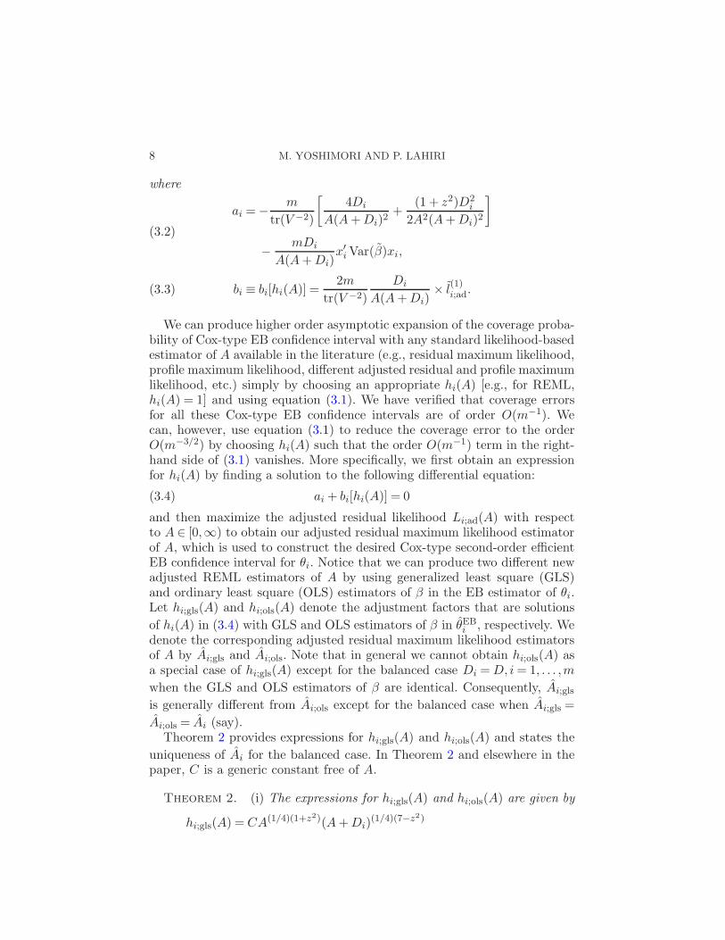
where
ai =− m
tr(V −2)
[4Di
A(A+Di)2+
(1 + z2)D2i
2A2(A+Di)2
]
(3.2)
− mDi
A(A+Di)x′iVar(β)xi,
bi ≡ bi[hi(A)] =2m
tr(V −2)
Di
A(A+Di)× l
(1)i;ad.(3.3)
We can produce higher order asymptotic expansion of the coverage proba-bility of Cox-type EB confidence interval with any standard likelihood-basedestimator of A available in the literature (e.g., residual maximum likelihood,profile maximum likelihood, different adjusted residual and profile maximumlikelihood, etc.) simply by choosing an appropriate hi(A) [e.g., for REML,hi(A) = 1] and using equation (3.1). We have verified that coverage errorsfor all these Cox-type EB confidence intervals are of order O(m−1). Wecan, however, use equation (3.1) to reduce the coverage error to the orderO(m−3/2) by choosing hi(A) such that the order O(m−1) term in the right-hand side of (3.1) vanishes. More specifically, we first obtain an expressionfor hi(A) by finding a solution to the following differential equation:
ai + bi[hi(A)] = 0(3.4)
and then maximize the adjusted residual likelihood Li;ad(A) with respectto A ∈ [0,∞) to obtain our adjusted residual maximum likelihood estimatorof A, which is used to construct the desired Cox-type second-order efficientEB confidence interval for θi. Notice that we can produce two different newadjusted REML estimators of A by using generalized least square (GLS)and ordinary least square (OLS) estimators of β in the EB estimator of θi.Let hi;gls(A) and hi;ols(A) denote the adjustment factors that are solutions
of hi(A) in (3.4) with GLS and OLS estimators of β in θEBi , respectively. Wedenote the corresponding adjusted residual maximum likelihood estimatorsof A by Ai;gls and Ai;ols. Note that in general we cannot obtain hi;ols(A) asa special case of hi;gls(A) except for the balanced case Di =D, i= 1, . . . ,m
when the GLS and OLS estimators of β are identical. Consequently, Ai;gls
is generally different from Ai;ols except for the balanced case when Ai;gls =
Ai;ols = Ai (say).Theorem 2 provides expressions for hi;gls(A) and hi;ols(A) and states the
uniqueness of Ai for the balanced case. In Theorem 2 and elsewhere in thepaper, C is a generic constant free of A.
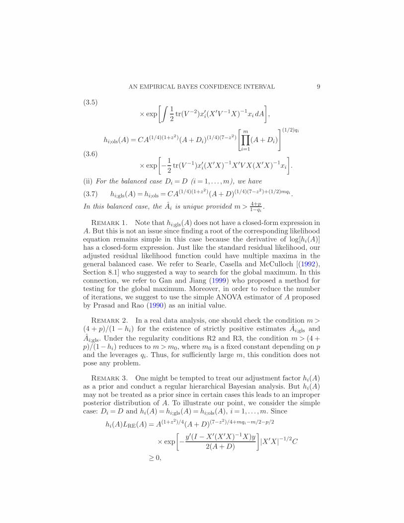
Theorem 2. (i) The expressions for hi;gls(A) and hi;ols(A) are given by
hi;gls(A) = CA(1/4)(1+z2)(A+Di)(1/4)(7−z2)
AN EMPIRICAL BAYES CONFIDENCE INTERVAL 9
(3.5)
× exp
[∫1
2tr(V −2)x′i(X
′V −1X)−1xi dA
],
hi;ols(A) = CA(1/4)(1+z2)(A+Di)(1/4)(7−z2)
[m∏
i=1
(A+Di)
](1/2)qi
(3.6)
× exp
[−1
2tr(V −1)x′i(X
′X)−1X ′V X(X ′X)−1xi
].
(ii) For the balanced case Di =D (i= 1, . . . ,m), we have
In this balanced case, the Ai is unique provided m> 4+p1−qi
.
Remark 1. Note that hi;gls(A) does not have a closed-form expression inA. But this is not an issue since finding a root of the corresponding likelihoodequation remains simple in this case because the derivative of log[hi(A)]has a closed-form expression. Just like the standard residual likelihood, ouradjusted residual likelihood function could have multiple maxima in thegeneral balanced case. We refer to Searle, Casella and McCulloch [(1992),Section 8.1] who suggested a way to search for the global maximum. In thisconnection, we refer to Gan and Jiang (1999) who proposed a method fortesting for the global maximum. Moreover, in order to reduce the numberof iterations, we suggest to use the simple ANOVA estimator of A proposedby Prasad and Rao (1990) as an initial value.
Remark 2. In a real data analysis, one should check the condition m>(4 + p)/(1 − hi) for the existence of strictly positive estimates Ai;gls and
Ai;gls. Under the regularity conditions R2 and R3, the condition m> (4 +p)/(1−hi) reduces to m>m0, where m0 is a fixed constant depending on pand the leverages qi. Thus, for sufficiently large m, this condition does notpose any problem.
Remark 3. One might be tempted to treat our adjustment factor hi(A)as a prior and conduct a regular hierarchical Bayesian analysis. But hi(A)may not be treated as a prior since in certain cases this leads to an improperposterior distribution of A. To illustrate our point, we consider the simplecase: Di =D and hi(A) = hi;gls(A) = hi;ols(A), i= 1, . . . ,m. Since
hi(A)LRE(A) =A(1+z2)/4(A+D)(7−z2)/4+mqi−m/2−p/2
× exp
[−y′(I −X ′(X ′X)−1X)y
2(A+D)
]|X ′X|−1/2C
≥ 0,
10 M. YOSHIMORI AND P. LAHIRI
under the regularity conditions, and exp[−y′(I−X′(X′X)−1X)y2(A+D) ] and A/(A+D)
are increasing monotone functions of A, there exists s <∞ such that
1− exp
[−y′(I −X ′(X ′X)−1X)y
2(s+D)
]<
1
2
and
1− s
s+D<
1
2.
Using the above results, we have∫ ∞
0hi(A)LRE dA≥C
∫ ∞
s(A+D)2+1/2[mqi+p]−m/2 dA,(3.8)
if m> 4+p1−qi
. Hence, if −1≤ 2 + 1/2[mqi + p]−m/2≤ 0, the right-hand side
of the above equation is infinite, even if m> 4+p1−qi
. Thus, in this case hi(A)
cannot be treated as a prior since∫∞0 hi(A)LRE dA =∞ in case −1 ≤ 2 +
1/2[mqi + p]−m/2≤ 0.
We now propose two empirical Bayes confidence intervals for θi:
IY Li (Ai;h) : θ
EBi (Ai;h)± zα/2σi(Ai;h),
where h= gls,ols. Since σi(Ai;h)<√Di (h= gls,ols), the length of our pro-
posed Cox-type EB intervals, like the original Cox EB interval ICoxi (AANOVA),
are always shorter than that of the direct interval IDi . The following theo-rem compares the lengths of Cox EB confidence intervals of θi when A isestimated by ARE, Ai;gls and Ai;ols.
Theorem 3. Under the regularity conditions R2–R4 and m> (4 + p)/(1− qi), we have
Length of ICoxi (ARE)≤ Length of IY L
i (Ai;gls)≤ Length of IY Li (Ai;ols).
The following theorem provides the higher order asymptotic properties ofa general class of adjusted residual maximum likelihood estimators of A.
Theorem 4. Under regularity conditions R1–R5, we have:
(i) E[Ahi−A] = 2
tr(V −1)l(1)i,ad(A) +O(m−3/2),
(ii) E(Ahi−A)2 = 2
tr(V −1)+O(m−3/2).
Corollary to Theorem 4. Under regularity conditions R2–R5, wehave:
AN EMPIRICAL BAYES CONFIDENCE INTERVAL 11
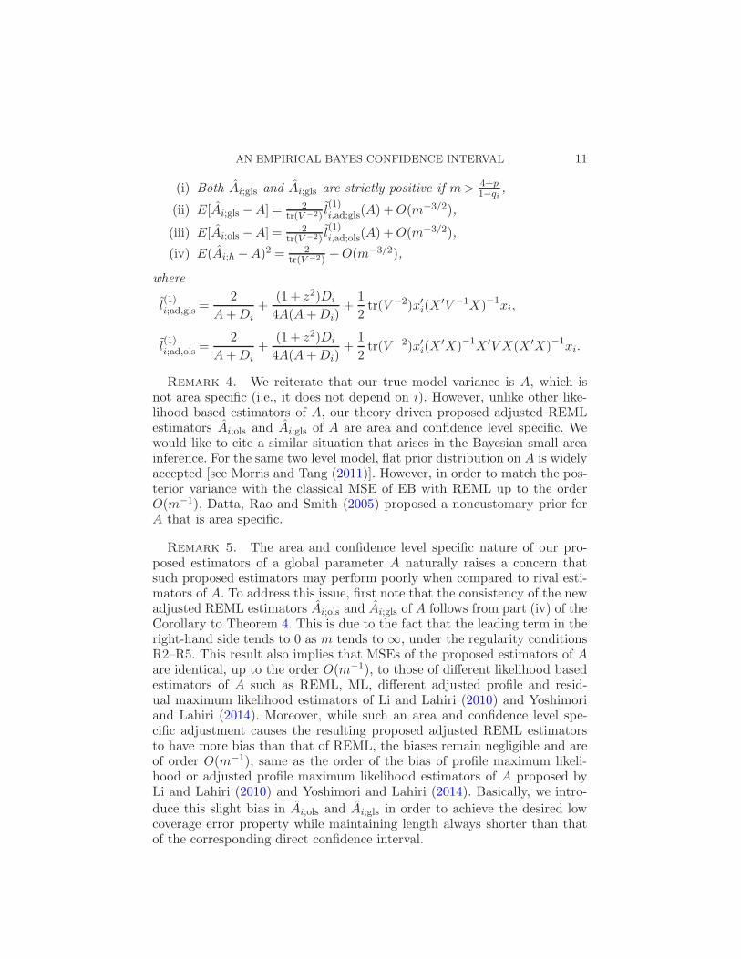
(i) Both Ai;gls and Ai;gls are strictly positive if m> 4+p1−qi
,
(ii) E[Ai;gls −A] = 2tr(V −2)
l(1)i,ad;gls(A) +O(m−3/2),
(iii) E[Ai;ols −A] = 2tr(V −2) l
(1)i,ad;ols(A) +O(m−3/2),
(iv) E(Ai;h −A)2 = 2tr(V −2)
+O(m−3/2),
where
l(1)i;ad,gls =
2
A+Di+
(1+ z2)Di
4A(A+Di)+
1
2tr(V −2)x′i(X
′V −1X)−1xi,
l(1)i;ad,ols =
2
A+Di+
(1+ z2)Di
4A(A+Di)+
1
2tr(V −2)x′i(X
′X)−1X ′V X(X ′X)−1xi.
Remark 4. We reiterate that our true model variance is A, which isnot area specific (i.e., it does not depend on i). However, unlike other like-lihood based estimators of A, our theory driven proposed adjusted REMLestimators Ai;ols and Ai;gls of A are area and confidence level specific. Wewould like to cite a similar situation that arises in the Bayesian small areainference. For the same two level model, flat prior distribution on A is widelyaccepted [see Morris and Tang (2011)]. However, in order to match the pos-terior variance with the classical MSE of EB with REML up to the orderO(m−1), Datta, Rao and Smith (2005) proposed a noncustomary prior forA that is area specific.
Remark 5. The area and confidence level specific nature of our pro-posed estimators of a global parameter A naturally raises a concern thatsuch proposed estimators may perform poorly when compared to rival esti-mators of A. To address this issue, first note that the consistency of the newadjusted REML estimators Ai;ols and Ai;gls of A follows from part (iv) of theCorollary to Theorem 4. This is due to the fact that the leading term in theright-hand side tends to 0 as m tends to ∞, under the regularity conditionsR2–R5. This result also implies that MSEs of the proposed estimators of Aare identical, up to the order O(m−1), to those of different likelihood basedestimators of A such as REML, ML, different adjusted profile and resid-ual maximum likelihood estimators of Li and Lahiri (2010) and Yoshimoriand Lahiri (2014). Moreover, while such an area and confidence level spe-cific adjustment causes the resulting proposed adjusted REML estimatorsto have more bias than that of REML, the biases remain negligible and areof order O(m−1), same as the order of the bias of profile maximum likeli-hood or adjusted profile maximum likelihood estimators of A proposed byLi and Lahiri (2010) and Yoshimori and Lahiri (2014). Basically, we intro-
duce this slight bias in Ai;ols and Ai;gls in order to achieve the desired lowcoverage error property while maintaining length always shorter than thatof the corresponding direct confidence interval.
12 M. YOSHIMORI AND P. LAHIRI
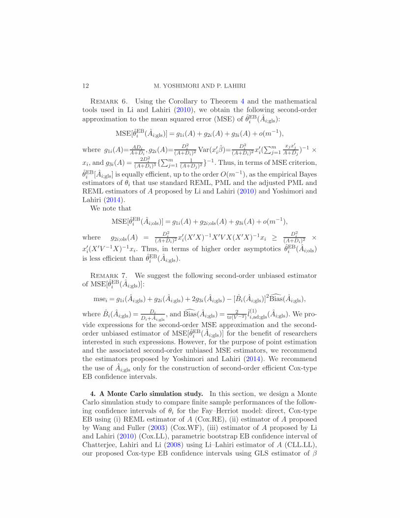
Remark 6. Using the Corollary to Theorem 4 and the mathematicaltools used in Li and Lahiri (2010), we obtain the following second-order
approximation to the mean squared error (MSE) of θEBi (Ai;gls):
θEBi [Ai;gls] is equally efficient, up to the order O(m−1), as the empirical Bayesestimators of θi that use standard REML, PML and the adjusted PML andREML estimators of A proposed by Li and Lahiri (2010) and Yoshimori andLahiri (2014).
vide expressions for the second-order MSE approximation and the second-order unbiased estimator of MSE[θEBi (Ai;gls)] for the benefit of researchersinterested in such expressions. However, for the purpose of point estimationand the associated second-order unbiased MSE estimators, we recommendthe estimators proposed by Yoshimori and Lahiri (2014). We recommend
the use of Ai;gls only for the construction of second-order efficient Cox-typeEB confidence intervals.
4. A Monte Carlo simulation study. In this section, we design a MonteCarlo simulation study to compare finite sample performances of the follow-ing confidence intervals of θi for the Fay–Herriot model: direct, Cox-typeEB using (i) REML estimator of A (Cox.RE), (ii) estimator of A proposedby Wang and Fuller (2003) (Cox.WF), (iii) estimator of A proposed by Liand Lahiri (2010) (Cox.LL), parametric bootstrap EB confidence interval ofChatterjee, Lahiri and Li (2008) using Li–Lahiri estimator of A (CLL.LL),our proposed Cox-type EB confidence intervals using GLS estimator of β
AN EMPIRICAL BAYES CONFIDENCE INTERVAL 13
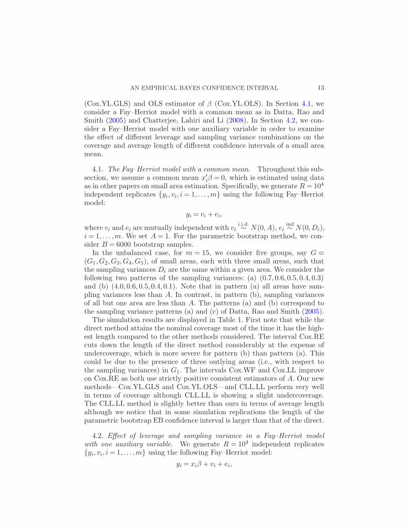
(Cox.YL.GLS) and OLS estimator of β (Cox.YL.OLS). In Section 4.1, weconsider a Fay–Herriot model with a common mean as in Datta, Rao andSmith (2005) and Chatterjee, Lahiri and Li (2008). In Section 4.2, we con-sider a Fay–Herriot model with one auxiliary variable in order to examinethe effect of different leverage and sampling variance combinations on thecoverage and average length of different confidence intervals of a small areamean.
4.1. The Fay–Herriot model with a common mean. Throughout this sub-section, we assume a common mean x′iβ = 0, which is estimated using dataas in other papers on small area estimation. Specifically, we generate R= 104
independent replicates {yi, vi, i= 1, . . . ,m} using the following Fay–Herriotmodel:
yi = vi + ei,
where vi and ei are mutually independent with vii.i.d.∼ N(0,A), ei
ind∼ N(0,Di),i = 1, . . . ,m. We set A= 1. For the parametric bootstrap method, we con-sider B = 6000 bootstrap samples.
In the unbalanced case, for m = 15, we consider five groups, say G ≡(G1,G2,G3,G4,G5), of small areas, each with three small areas, such thatthe sampling variances Di are the same within a given area. We consider thefollowing two patterns of the sampling variances: (a) (0.7,0.6,0.5,0.4,0.3)and (b) (4.0,0.6,0.5,0.4,0.1). Note that in pattern (a) all areas have sam-pling variances less than A. In contrast, in pattern (b), sampling variancesof all but one area are less than A. The patterns (a) and (b) correspond tothe sampling variance patterns (a) and (c) of Datta, Rao and Smith (2005).
The simulation results are displayed in Table 1. First note that while thedirect method attains the nominal coverage most of the time it has the high-est length compared to the other methods considered. The interval Cox.REcuts down the length of the direct method considerably at the expense ofundercoverage, which is more severe for pattern (b) than pattern (a). Thiscould be due to the presence of three outlying areas (i.e., with respect tothe sampling variances) in G1. The intervals Cox.WF and Cox.LL improveon Cox.RE as both use strictly positive consistent estimators of A. Our newmethods—Cox.YL.GLS and Cox.YL.OLS—and CLL.LL perform very wellin terms of coverage although CLL.LL is showing a slight undercoverage.The CLL.LL method is slightly better than ours in terms of average lengthalthough we notice that in some simulation replications the length of theparametric bootstrap EB confidence interval is larger than that of the direct.
4.2. Effect of leverage and sampling variance in a Fay–Herriot modelwith one auxiliary variable. We generate R = 104 independent replicates{yi, vi, i= 1, . . . ,m} using the following Fay–Herriot model:
yi = xiβ + vi + ei,
14 M. YOSHIMORI AND P. LAHIRI
where vi and ei are mutually independent with vii.i.d.∼ N(0,A), ei
ind∼ N(0,Di),i = 1, . . . ,m. We set A= 1. For the parametric bootstrap method, we con-sider B = 6000 bootstrap samples.
In this subsection, we examine the effects of leverage and sampling vari-ance on different confidence intervals for θi. We consider six different (lever-age, sampling variance) patterns of the first area using leverages (0.07,0.22,0.39) and sampling variances D1 = (1,5,10). For the remaining 14 areas, weassume equal small sampling variances Dj = 0.01, j ≥ 2 and same leverage.Since the total leverage for all the areas must be 1, we obtain the commonleverage for the other areas from the knowledge of leverage for the first area.
In Table 2, we report the coverages and average lengths for all the com-peting methods for the first area for all the six patterns. We do not reportthe results for the remaining 14 areas since they are similar, as expected,due to small sampling variances in those areas. The use of strictly posi-tive consistent estimators of A such as WF and LL help bringing coverageof the Cox-type EB confidence interval closer to the nominal coverage of95% than the one based on REML. For large sampling variances and lever-ages, the Cox-type EB confidence intervals based on REML, WF and LLmethods have generally shorter length than ours or parametric bootstrapconfidence interval but only at the expense of severe undercoverage. Oursimulation results show that our proposed Cox.YL.GLS could perform betterthan Cox.YL.OLS and is very competitive to the more computer intensiveCLL.LL method.
5. Concluding remarks. In this paper, we put forward a new simple ap-proach for constructing second-order efficient empirical Bayes confidenceinterval for a small area mean using a carefully devised adjusted residualmaximum likelihood estimator of the model variance in the well-known Coxempirical Bayes confidence interval. Our simulation results show that theproposed method performs much better than the direct or Cox EB con-fidence intervals with different standard likelihood based estimators of themodel variance. In our simulation, the parametric bootstrap empirical Bayesconfidence interval also performs well and it generally produces intervalsshorter than direct confidence intervals on the average. However, to the bestof our knowledge, there is no analytical result that shows that the paramet-ric bootstrap empirical Bayes confidence interval is always shorter than thedirect interval. In fact, in our simulation we found cases where the lengthof parametric bootstrap empirical Bayes confidence interval is higher thanthat of the direct. In order to obtain good parametric bootstrap empiricalBayes confidence intervals, choices of the estimator of A and the bootstrapreplication B appear to be important. To limit the computing time, we haveconsidered a simple simulation setting with m= 15. During the course of our
AN
EMPIR
ICALBAYESCONFID
ENCE
INTERVAL
15
Table 1
Simulation results for Section 4.1: Simulated coverage and average length (in parenthesis) of different confidence intervals of small areameans; nominal coverage is 95%
Pattern G Cox.WF Cox.RE Cox.LL CLL.LL Cox.YL.GLS Cox.YL.OLS Direct
Simulation results for Section 4.2: Simulated coverage and average length (in parenthesis) of different confidence intervals for the firstsmall area mean for different combinations of leverage and sampling variance of the first area; nominal coverage is 95%
Leverage D1 Cox.WF Cox.RE Cox.LL CLL.LL Cox.YL.gls Cox.YL.ols Direct
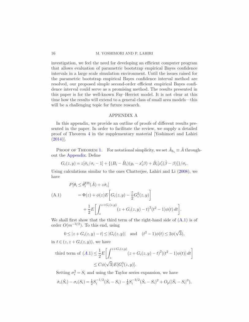
investigation, we feel the need for developing an efficient computer programthat allows evaluation of parametric bootstrap empirical Bayes confidenceintervals in a large scale simulation environment. Until the issues raised forthe parametric bootstrap empirical Bayes confidence interval method areresolved, our proposed simple second-order efficient empirical Bayes confi-dence interval could serve as a promising method. The results presented inthis paper is for the well-known Fay–Herriot model. It is not clear at thistime how the results will extend to a general class of small area models—thiswill be a challenging topic for future research.
APPENDIX A
In this appendix, we provide an outline of proofs of different results pre-sented in the paper. In order to facilitate the review, we supply a detailedproof of Theorem 4 in the supplementary material [Yoshimori and Lahiri(2014)].
Proof of Theorem 1. For notational simplicity, we set Ahi≡ A through-
Setting σ2i = Si and using the Taylor series expansion, we have
σi(Si)− σi(Si) =12S
−1/2i (Si − Si)− 1
8S−3/2i (Si − Si)
2 +Op(|Si − Si|3),
AN EMPIRICAL BAYES CONFIDENCE INTERVAL 17
so that
σi(Si)
σi(Si)− 1 =
1
2Si(Si − Si)−
1
8S2i
(Si − Si)2 +RA1.
Using
Bi −Bi =−(A−A)Di
(A+Di)2+ (A−A)2
Di
(A+Di)3+RA2,
σ2i − σ2
i = (A−A)D2
i
(A+Di)2− (A−A)2
D2i
(A+Di)3+RA3,
we can write Gi(z, y) =G1i(y) +G2i(z, y), where
G1i(y) =1√mu1i +
1
mu2i +RA4,
G2i(z, y) = z
[1√mv1i +
1
mv2i
]+RA5,
with
u1i =√mσ−1
i
[Bix
′i(β − β) + (A−A)
Di
(A+Di)2(yi − x′iβ)
],
u2i =mσ−1i
[−(A−A)2
Di
(A+Di)3(yi − x′iβ)
+ (A−A)Di
(A+Di)2Bix
′i(β − β)
],
v1i =√m
B2i
2σ2i
(A−A),
v2i =m
[− 1
2σ2i
B2i
A+Di(A−A)2 − 1
8σ4i
(A−A)2B4i
].
Using the fact that E[|A−A|k] =O(m−3/2) for k ≥ 3 [this can be provedusing the mathematical tools used in Li and Lahiri (2010) and Das, Jiangand Rao (2004)], we have, for k = 1,2,3,4,5 and large m,
Using Lemma 1, given below, and considerable algebra, we show that
ai =E[2v2i − u21i − z2v21i] and bi = 2√mE[v1i].
This completes the proof of equation (3.1). �
Lemma 1. Under the regularity conditions R1–R5, we have
E[v21i(A)] =m
tr(V −2)
D2i
2A2(A+Di)2+O(m−1/2),(A.3)
E[v2i(A)] =− m
tr(V −2)
[Di
A(A+Di)2+
D2i
4A2(A+Di)2
]
(A.4)+O(m−1/2),
AN EMPIRICAL BAYES CONFIDENCE INTERVAL 19
E[u21i(A)] =mDi
A(A+Di)
[E[{x′iβ − β)}2] + Di
A(A+Di)22
tr(V −2)
]
(A.5)+O(m−1/2),
E[v1i(A)] =
√m
tr(V −2)
Di
A(A+Di)l(1)i;ad +O(m−1).(A.6)
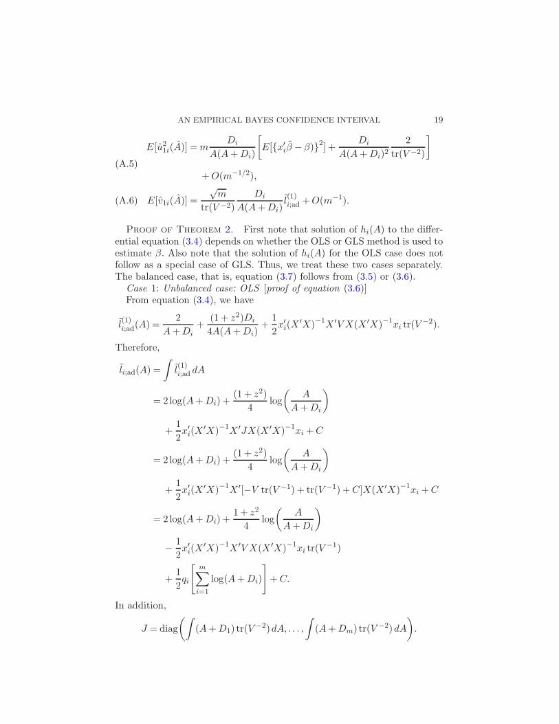
Proof of Theorem 2. First note that solution of hi(A) to the differ-ential equation (3.4) depends on whether the OLS or GLS method is used toestimate β. Also note that the solution of hi(A) for the OLS case does notfollow as a special case of GLS. Thus, we treat these two cases separately.The balanced case, that is, equation (3.7) follows from (3.5) or (3.6).
Case 1: Unbalanced case: OLS [proof of equation (3.6)]From equation (3.4), we have
l(1)i;ad(A) =
2
A+Di+
(1+ z2)Di
4A(A+Di)+
1
2x′i(X
′X)−1X ′V X(X ′X)−1xi tr(V−2).
Therefore,
li;ad(A) =
∫l(1)i;ad dA
= 2 log(A+Di) +(1 + z2)
4log
(A
A+Di
)
+1
2x′i(X
′X)−1X ′JX(X ′X)−1xi +C
= 2 log(A+Di) +(1 + z2)
4log
(A
A+Di
)
+1
2x′i(X
′X)−1X ′[−V tr(V −1) + tr(V −1) +C]X(X ′X)−1xi +C
= 2 log(A+Di) +1+ z2
4log
(A
A+Di
)
− 1
2x′i(X
′X)−1X ′V X(X ′X)−1xi tr(V−1)
+1
2qi
[m∑
i=1
log(A+Di)
]+C.
In addition,
J = diag
(∫(A+D1) tr(V
−2)dA, . . . ,
∫(A+Dm) tr(V −2)dA
).
20 M. YOSHIMORI AND P. LAHIRI
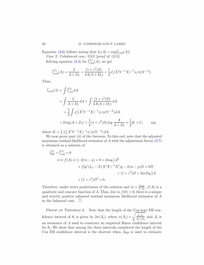
Equation (3.6) follows noting that hi(A) = exp[li;ad(A)].Case 2: Unbalanced case: GLS [proof of (3.5)]
Solving equation (3.4) for l(1)i;ad(A), we get
l(1)i;ad(A) =
2
A+Di+
(1+ z2)Di
4A(A+Di)+
1
2x′i(X
′V −1X)−1xi tr(V−2).
Thus,
li;ad(A) =
∫l(1)i;ad dA
=
∫2
A+DidA+
∫(1 + z2)Di
4A(A+Di)dA
+1
2
∫x′i(X
′V −1X)−1xi tr(V−2)dA
= 2 log(A+Di) +1
4(1 + z2)Di log
A
A+Di+
1
2K +C, say,
where K =∫x′i(X
′V −1X)−1xi tr(V−2)dA.
We now prove part (ii) of the theorem. To this end, note that the adjustedmaximum residual likelihood estimator of A with the adjustment factor (3.7)is obtained as a solution of
l(1)RE + l
(1)i,ad = 0
⇐⇒ f(A)≡ {−2(m− p) + 8+ 2mqi}A2
+ {2y′(Im −X(X ′X)−1X ′)y − 2(m− p)D+ 8D
+ (1+ z2)D+2mDqi}A+ (1+ z2)D2 = 0.
Therefore, under strict positiveness of the solution and m> 4+p1−qi
, f(A) is a
quadratic and concave function of A. Thus, due to f(0)> 0, there is a uniqueand strictly positive adjusted residual maximum likelihood estimator of Ain the balanced case. �
Proof of Theorem 3. Note that the length of the Cox-type EB con-
fidence interval of θi is given by 2σ(Ai), where σ(Ai) =
√AiDi
Ai+Diand Ai is
an estimator of A used to construct an empirical Bayes confidence intervalfor θi. We show that among the three intervals considered the length of theCox EB confidence interval is the shortest when ARE is used to estimate
AN EMPIRICAL BAYES CONFIDENCE INTERVAL 21
A, followed by Ai,gls, and Ai,ols. Since σ(Ai) is a monotonically increasing
function of Ai, it suffices to show that
ARE ≤ Ai,gls ≤ Ai,ols.
Note that
l(1)RE(ARE) = 0,
l(1)RE(Ai,gls) + l
(1)i;ad,gls(Ai,gls) = 0,
l(1)RE(Ai,ols) + l
(1)i;ad,ols(Ai,ols) = 0,
l(2)RE(A) + l
(2)i;ad(A)< 0,
where A ∈ {ARE, Ai,gls, Ai,ols} and ARE is a solution to the REML estimation
equation. Hence, ARE is always larger than Ai,gls or Ai,gls using the facts
that ARE = max{0, ARE} and Ai,gls or Ai,gls are strictly positive if m >(4 + p)/(1− qi).
Finally, using that 0< l(1)i;ad,gls ≤ l
(1)i;ad,ols for A≥ 0, we have the result. �
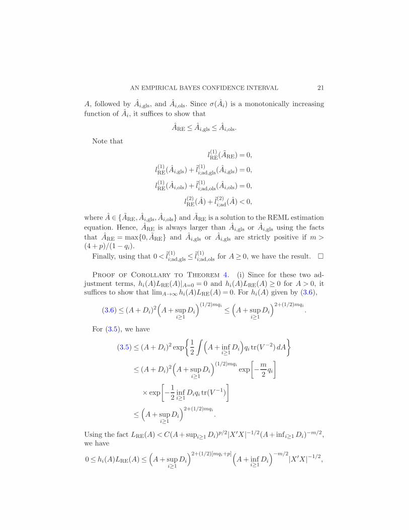
Proof of Corollary to Theorem 4. (i) Since for these two ad-justment terms, hi(A)LRE(A)|A=0 = 0 and hi(A)LRE(A) ≥ 0 for A > 0, itsuffices to show that limA→∞ hi(A)LRE(A) = 0. For hi(A) given by (3.6),
(3.6)≤ (A+Di)2(A+ sup
i≥1Di
)(1/2)mqi ≤(A+ sup
i≥1Di
)2+(1/2)mqi.
For (3.5), we have
(3.5)≤ (A+Di)2 exp
{1
2
∫ (A+ inf
i≥1Di
)qi tr(V
−2)dA
}
≤ (A+Di)2(A+ sup
i≥1Di
)(1/2)mqiexp
[−m
2qi
]
× exp
[−1
2infi≥1
Diqi tr(V−1)
]
≤(A+ sup
i≥1Di
)2+(1/2)mqi.
Using the fact LRE(A)<C(A+supi≥1Di)p/2|X ′X|−1/2(A+infi≥1Di)
−m/2,we have
0≤ hi(A)LRE(A)≤(A+ sup
i≥1Di
)2+(1/2)[mqi+p](A+ inf
i≥1Di
)−m/2|X ′X|−1/2,
22 M. YOSHIMORI AND P. LAHIRI
so that, under mild regularity conditions,
0≤ limA→∞
hi(A)LRE(A) = limA→∞
A2+(1/2)[mqi+p−m].
Thus, if 2 + 12 [mqi + p−m]< 0, we have
limA→∞
hi(A)LRE(A) = 0.
We first show that Ai;gls and Ai;gls satisfy the regularity conditions of
Theorem 3. Since 0<A<∞, we claim that lki,ad(A) =O(1) (k = 1,2,3), forlarge m, for both the GLS and OLS estimators of β using the following facts.
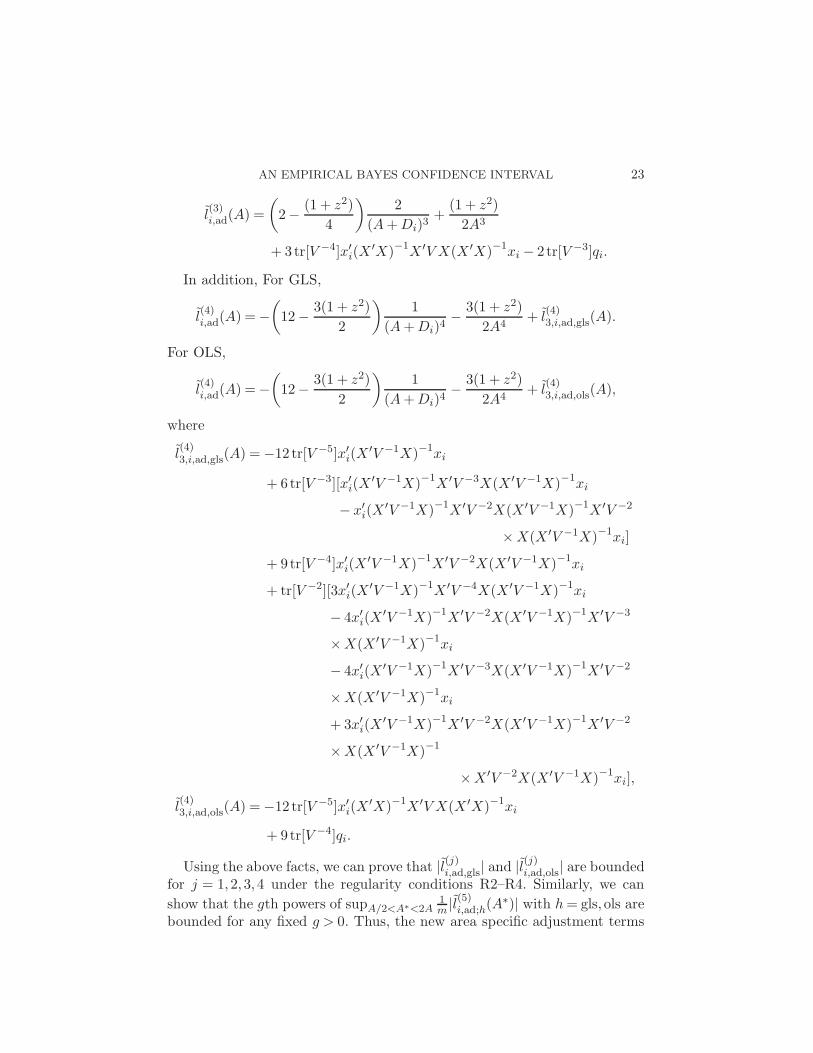
Using the above facts, we can prove that |l(j)i,ad,gls| and |l(j)i,ad,ols| are boundedfor j = 1,2,3,4 under the regularity conditions R2–R4. Similarly, we can
show that the gth powers of supA/2<A∗<2A1m |l(5)i,ad;h(A
∗)| with h= gls,ols arebounded for any fixed g > 0. Thus, the new area specific adjustment terms
24 M. YOSHIMORI AND P. LAHIRI
satisfy the regularity condition R1. Thus, an application of Theorem 4 leadsto (ii)–(iv) of the Corollary to Theorem 4. �
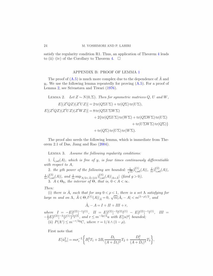
APPENDIX B: PROOF OF LEMMA 1
The proof of (A.5) is much more complex due to the dependence of A andyi. We use the following lemma repeatedly for proving (A.5). For a proof ofLemma 2, see Srivastava and Tiwari (1976).
Lemma 2. Let Z ∼N(0,Σ). Then for symmetric matrices Q, U and W ,
E[(Z ′QZ)(Z ′UZ)] = 2 tr(QΣUΣ)+ tr(QΣ)tr(UΣ),
E[(Z ′QZ)(Z ′UZ)(Z ′WZ)] = 8 tr(QΣUΣWΣ)
+ 2{tr(QΣUΣ)tr(WΣ)+ tr(QΣWΣ)tr(UΣ)
+ tr(UΣWΣ)tr(QΣ)}+ tr(QΣ)tr(UΣ)tr(WΣ).
The proof also needs the following lemma, which is immediate from The-orem 2.1 of Das, Jiang and Rao (2004).
Lemma 3. Assume the following regularity conditions:
1. li,ad(A), which is free of y, is four times continuously differentiablewith respect to A,
2. the gth power of the following are bounded: 1√m|l(1)i,ad(A)|, 1
m |l(2)i,ad(A)|,1m |l(3)i,ad(A)|, and 1
m supA/2<A<2A |l(4)i,ad(A)|A=A| (fixed g > 0),
3. A ∈Θ0, the interior of Θ, that is, 0<A<∞.
Then:(i) there is Ai such that for any 0< ρ < 1, there is a set Λ satisfying for
large m and on Λ, A ∈Θ, l(1)(A)|A = 0,√m|Ai −A|<m(1−ρ)/2, and
Ai −A= I + II + III + r,
where I = −E[l(2)]−1l(1), II = E[l(2)]−2l(2)l(1) − E[l(2)]−1l(1), III =−1
2E[l(2)]−3{l(1)}2l(3), and r ≤m−3ρ/2u with E[|u|g] bounded;(ii) P (Λc)≤m−τ/2gC, where τ = 1/4 ∧ (1− ρ).
First note that
E[u21i] =mσ−2i
{B2
i T1 +2BiDi
(A+Di)2T2 +
D2i
(A+Di)4T3
},
AN EMPIRICAL BAYES CONFIDENCE INTERVAL 25
where T1 = E[x′i(β − β)2], T2 = E[(A − A)x′i(β − β)(yi − x′iβ)] and T3 =
E[(A−A)2(yi − x′iβ)2]. We now simplify these three terms.
We first prove that
E[T1] = x′iVar(β)xi +O(m−2),(B.1)
where Var(β) = (X ′X)−1X ′V X(X ′X)−1 if β is the OLS estimator of β and(X ′V −1X)−1 if β is the GLS estimator of β.
Let H(1)s be the matrix with (i, j) components given by
supA/2<A∗<2A
{∂H
∂A
∣∣∣∣A=A∗
}
(i,j)
,
where Q(i,j) is (i, j) component of a matrix Q. Under the regularity con-
ditions R3–R4, we can show that the components of H(1)s are bounded
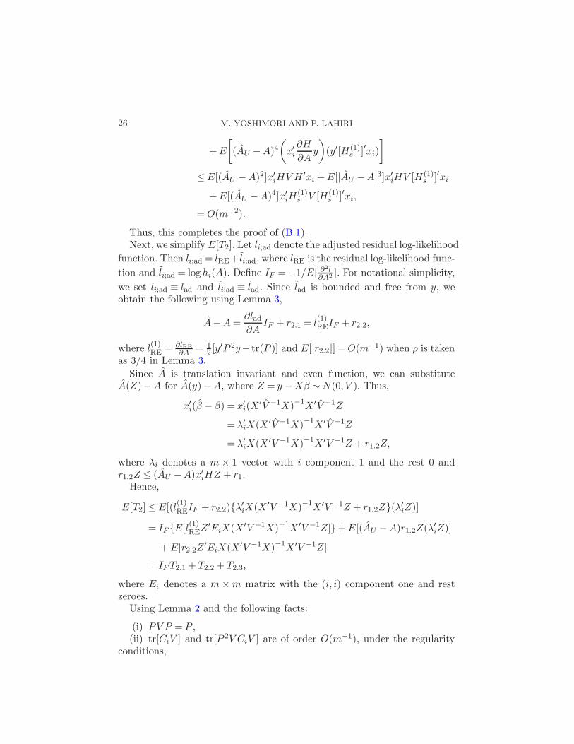
and of order O(m−1) using an argument similar to that given in Propo-sition 3.2 of Das, Jiang and Rao (2004). Using the facts that HX = 0,x′iHV H ′xi =O(m−1), we have
E[{x′i(β − β)}2]≤ E[(AU −A)2(x′iHy)(y′H ′xi)]
+ 2E[(AU −A)3(x′iHy)(y′[H(1)s ]′xi)]
26 M. YOSHIMORI AND P. LAHIRI
+E
[(AU −A)4
(x′i∂H
∂Ay
)(y′[H(1)
s ]′xi)
]
≤ E[(AU −A)2]x′iHV H ′xi +E[|AU −A|3]x′iHV [H(1)s ]′xi
+E[(AU −A)4]x′iH(1)s V [H(1)
s ]′xi,
=O(m−2).
Thus, this completes the proof of (B.1).Next, we simplify E[T2]. Let li;ad denote the adjusted residual log-likelihood
function. Then li;ad = lRE+ li;ad, where lRE is the residual log-likelihood func-
tion and li;ad = loghi(A). Define IF =−1/E[ ∂2l
∂A2 ]. For notational simplicity,
we set li;ad ≡ lad and li;ad ≡ lad. Since lad is bounded and free from y, weobtain the following using Lemma 3,
A−A=∂lad∂A
IF + r2.1 = l(1)REIF + r2.2,
where l(1)RE = ∂lRE
∂A = 12 [y
′P 2y− tr(P )] and E[|r2.2|] =O(m−1) when ρ is takenas 3/4 in Lemma 3.
Since A is translation invariant and even function, we can substituteA(Z)−A for A(y)−A, where Z = y −Xβ ∼N(0, V ). Thus,
x′i(β − β) = x′i(X′V −1X)−1X ′V −1Z
= λ′iX(X ′V −1X)−1X ′V −1Z
= λ′iX(X ′V −1X)−1X ′V −1Z + r1.2Z,
where λi denotes a m × 1 vector with i component 1 and the rest 0 andr1.2Z ≤ (AU −A)x′iHZ + r1.
Hence,
E[T2]≤E[(l(1)REIF + r2.2){λ′
iX(X ′V −1X)−1X ′V −1Z + r1.2Z}(λ′iZ)]
= IF {E[l(1)REZ
′EiX(X ′V −1X)−1X ′V −1Z]}+E[(AU −A)r1.2Z(λ′iZ)]
+E[r2.2Z′EiX(X ′V −1X)−1X ′V −1Z]
= IFT2.1 + T2.2 + T2.3,
where Ei denotes a m×m matrix with the (i, i) component one and restzeroes.
Using Lemma 2 and the following facts:
(i) PV P = P ,(ii) tr[CiV ] and tr[P 2V CiV ] are of order O(m−1), under the regularity
conditions,
AN EMPIRICAL BAYES CONFIDENCE INTERVAL 27
we have
T2.1 =12{E[(Z ′P 2Z)(Z ′CiZ)]− tr[P ]E[Z ′CiZ]}
= tr[P 2V CiV ] + 12 tr[P
2V ] tr[CiV ]− 12 tr[P ] tr[CiV ]
=O(m−1),
where Ci =EiX(X ′V −1X)−1X ′V −1.Using λ′
i∂H∂A =O(m−1), we have
T2.2 =E[(AU −A)r1.2Z(λ′iZ)]
=E[(AU −A)2(λ′iXHZ)(λ′
iZ)] +E[(AU −A)r1(λ′iZ)]
≤E[(AU −A)2]E[Z ′H ′X ′EiZ] +E
[(AU −A)3
(λ′iX
∂H
∂A
∣∣∣∣A=A
Z
)(λ′
iZ)
]
=O(m−2).
Using E[|r2.2|] =O(m−1),
T2.3 =E[r2.2Z′CiZ]≤E[|r2.2|] tr[CiV ] =O(m−2).
Therefore,
E[T2]≤O(m−2).
Hence, using the above results and E[T2]≥O(m−2) with same calculation,we have
(i) PV P = P ,(ii) tr(EiV ) = (A+Di), and(iii) | tr(P k)− tr(V −k)|=O(1), for k ≥ 1,
28 M. YOSHIMORI AND P. LAHIRI
we have
Γ = {14E[(Z ′P 2Z)(Z ′P 2Z)(Z ′EiZ)]− 1
2E[(Z ′P 2Z)(Z ′EiZ)] tr[P ]
+ 14E[Z ′EiZ] tr[P ]2}
= 14 [8 tr(P
2V P 2EiV ) + 2{tr(P 2V P 2V ) tr(EiV ) + 2tr(P 2V EiV ) tr(P 2V )}
+ tr(P 2V )2 tr(EiV )]
− tr(P 2V EiV ) tr(P )− 12 tr(P
2V ) tr(EiV ) tr(P ) + 14 tr(P )2 tr(EiV )
= 2tr(P 3V EiV ) + 12 tr(P
2) tr(EiV ) = 12 tr(P
2) tr(EiV ) +O(1)
= 12 tr(V
−2)(A+Di) +O(1).
Hence,
E[T3] = I2F1
2tr(V −2)(A+Di) +O(m−2) =
2(A+Di)
tr(V −2)+O(m−2).(B.5)
Thus, we can show (A.5) using (B.1), (B.4) and (B.5).
Acknowledgments. M. Yoshimori conducted this research while visitingthe University of Maryland, College Park, USA, as a research scholar underthe supervison of the second author. The authors thank Professor YutakaKano for reading an earlier draft of the paper and making constructive com-ments. We are also grateful to three referees, an Associate Editor and Pro-fessor Runze Li, Coeditor, for making a number of constructive suggestions,which led to a significant improvement of our paper.
SUPPLEMENTARY MATERIAL
Supplemental proof (DOI: 10.1214/14-AOS1219SUPP; .pdf). We providea proof of Theorem 4.
REFERENCES
Basu, R., Ghosh, J. K. and Mukerjee, R. (2003). Empirical Bayes prediction intervalsin a normal regression model: Higher order asymptotics. Statist. Probab. Lett. 63 197–203. MR1986689
Bell, W. R., Basel, W., Cruse, C., Dalzell, L., Maples, J., Ohara, B. and Pow-
ers, D. (2007). Use of ACS data to produce SAIPE model-based estimates of povertyfor counties. Census report. U.S. Census Bureau, Washington, DC.
Carlin, B. P. and Louis, T. A. (1996). Bayes and Empirical Bayes Methods for DataAnalysis. Monographs on Statistics and Applied Probability 69. Chapman & Hall, Lon-don. MR1427749
Carter, G. M. and Rolph, J. F. (1974). Empirical Bayes methods applied to estimatingfire alarm probabilities. J. Amer. Statist. Assoc. 69 880–885.
Chatterjee, S., Lahiri, P. and Li, H. (2008). Parametric bootstrap approximation tothe distribution of EBLUP and related prediction intervals in linear mixed models.Ann. Statist. 36 1221–1245. MR2418655
Cox, D. R. (1975). Prediction intervals and empirical Bayes confidence intervals. In Per-spectives in Probability and Statistics (papers in Honour of M. S. Bartlett on the Oc-casion of His 65th Birthday) J. Gani, ed.) 47–55. Applied Probability Trust, Univ.Sheffield, Sheffield. MR0403046
Das, K., Jiang, J. and Rao, J. N. K. (2004). Mean squared error of empirical predictor.Ann. Statist. 32 818–840. MR2060179
Datta, G. S. and Lahiri, P. (2000). A unified measure of uncertainty of estimated bestlinear unbiased predictors in small area estimation problems. Statist. Sinica 10 613–627.MR1769758
Datta, G. S., Rao, J. N. K. and Smith, D. D. (2005). On measuring the variabil-ity of small area estimators under a basic area level model. Biometrika 92 183–196.MR2158619
Datta, G. S., Ghosh, M., Smith, D. D. and Lahiri, P. (2002). On an asymptotic theoryof conditional and unconditional coverage probabilities of empirical Bayes confidenceintervals. Scand. J. Stat. 29 139–152. MR1894387
Diao, L., Smith, D. D., Datta, G. S., Maiti, T. and Opsomer, J. D. (2014). Accurateconfidence interval estimation of small area parameters under the Fay–Herriot model.Scand. J. Stat. 41 497–515.
Efron, B. and Morris, C. N. (1975). Data analysis using Stein’s estimator and itsgeneralizations. J. Amer. Statist. Assoc. 70 311–319.
Fay, R. E. III and Herriot, R. A. (1979). Estimates of income for small places: Anapplication of James–Stein procedures to census data. J. Amer. Statist. Assoc. 74 269–277. MR0548019
Gan, L. and Jiang, J. (1999). A test for global maximum. J. Amer. Statist. Assoc. 94847–854. MR1723335
Hall, P. and Maiti, T. (2006). On parametric bootstrap methods for small area predic-tion. J. R. Stat. Soc. Ser. B Stat. Methodol. 68 221–238. MR2188983
Lahiri, P. and Li, H. (2009). Generalized maximum likelihood method in linearmixed models with an application in small area estimation. In Proceedings of theFederal Committee on Statistical Methodology Research Conference. Available athttp://www.fcsm.gov/events/papers2009.html.
Laird, N. M. and Louis, T. A. (1987). Empirical Bayes confidence intervals based onbootstrap samples. J. Amer. Statist. Assoc. 82 739–757. MR0909979
Li, H. and Lahiri, P. (2010). An adjusted maximum likelihood method for solving smallarea estimation problems. J. Multivariate Anal. 101 882–892. MR2584906
Morris, C. N. (1983a). Parametric empirical Bayes inference: Theory and applications.J. Amer. Statist. Assoc. 78 47–65. MR0696849
Morris, C. N. (1983b). Parametric empirical Bayes confidence intervals. In ScientificInference, Data Analysis, and Robustness (Madison, Wis., 1981) (G. E. P. Box, T.
Leonard and C. F. J. Wu, eds.). Publ. Math. Res. Center Univ. Wisconsin 48 25–50.Academic Press, Orlando, FL. MR0772762
Morris, C. N. and Tang, R. (2011). Estimating random effects via adjustment for densitymaximization. Statistical Sci. 26 271–287. MR2858514
Nandram, B. (1999). An empirical Bayes prediction interval for the finite populationmean of a small area. Statist. Sinica 9 325–343. MR1707843
Prasad, N. G. N. and Rao, J. N. K. (1990). The estimation of the mean squared errorof small-area estimators. J. Amer. Statist. Assoc. 85 163–171. MR1137362
Rao, J. N. K. (2003). Small Area Estimation. Wiley, Hoboken, NJ. MR1953089Sasase, Y. and Kubokawa, T. (2005). Asymptotic correction of empirical Bayes con-
fidence intervals and its application to small area estimation (in Japanese). J. JapanStatist. Soc. 35 27–54.
Searle, S. R., Casella, G. and McCulloch, C. E. (1992). Variance Components.Wiley, New York. MR1190470
Srivastava, V. K. and Tiwari, R. (1976). Evaluation of expectations of products ofstochastic matrices. Scand. J. Stat. 3 135–138. MR0518922
Wang, J. and Fuller, W. A. (2003). The mean squared error of small area predic-tors constructed with estimated area variances. J. Amer. Statist. Assoc. 98 716–723.MR2011685
Yoshimori, M. (2014). Numerical comparison between different prediction intervals usingEBLUP under the Fay–Herriot model. Comm. Statist. Simulation Comput. To appear.
Yoshimori, M. and Lahiri, P. (2014). Supplement to “A second-order efficient empiricalBayes confidence interval.” DOI:10.1214/14-AOS1219SUPP.
Yoshimori, M. and Lahiri, P. (2014). A new adjusted maximum likelihood method forthe Fay–Herriot small area model. J. Multivariate Anal. 124 281–294. MR3147326