Abstract A buried pipe extends over long distances and passes through soils with differentproperties. In the event of an earthquake, the same pipe experiences a variable ground motionalong its length. At bends, geometrically a more complicated problem exists where seismicwaves propagating in a certain direction affect pipe before and after bend differently. Studyingthese different effects is the subject of this paper. Two variants for modeling of pipe, a beammodel and a beam-shell hybrid model are examined. The surrounding soil is modeled withthe conventional springs in both models. A suitable boundary condition is introduced at theends of the system to simulate the far field. Effects of angle of incidence in the horizontaland vertical planes, angle of pipe bend, soil type, diameter to thickness ratio, and burialdepth ratio on pipe strains at bend are examined thoroughly. It is concluded that extensionalstrains are highest at bends and these strains increase with the angle of incidence with thevertical axis. The pipe strains attain their peaks when pipe bend is around 135◦ and exceedthe elastic limit in certain cases especially in stiffer soils, but remain below the rupture limit.Then equations for predicting the seismic response of the buried pipe at bend are developedusing the analytical data calculated above and regression analysis. It is shown that thesesemi-analytical equations predict the response with very good accuracy saving much timeand effort.
Keywords Buried pipe · Bend · Wave propagation · Hybrid model · Numerical analysis ·Semi-analytical equation
M. Saberi · F. Behnamfar (B) · M.VafaeianDepartment of Civil Engineering, Isfahan University of Technology,8415683111 Isfahan , Irane-mail: [email protected]
Categorizing piping systems among lifelines demonstrates importance of their appropriatebehaviour in maintaining societies’ safety and health. Because of its extension over a vastregion where it might cross active faults or liquefiable soils, a piping system is prone to a largerrisk compared to other facilities occupying small areas. Failure potential in earthquakes insuch a problem is quantified using permanent and transitional ground deformations. While thepermanent ground deformations generally originate from faulting, liquefaction, and sliding,the transitional deformations are produced by seismic waves propagating in the soil medium(Dash and Jain 2008).
Incidence of seismic waves on buried pipes can result in failures mainly as excessivetension and compression, and local and general buckling. As the seismic waves propagate inground, every two particles of soil vibrate out of phase. Due to this phenomenon and inter-action of soil and pipe at their interface, bending and longitudinal strains develop along pipe.Investigation on the seismic behavior of buried pipes dates back at least to 1967 when New-mark and his colleagues presented an approximate analysis method under wave propagation(Newmark 1968; American Society of Civil Engineers 1984; Berrones and Liu 2003). After-wards, various analytical and numerical procedures have been developed and tested by dif-ferent researchers. Within the closed form solutions derived, only a few are for bends and therest are specific to straight pipes. As of the analytical methods, Newmark ignored the effectsof the inertia force and pipe-soil interaction and assumed equal strains for ground and pipe.
Sakurai and Takahashi studied the role of inertia force on dynamic response of straightpipes and concluded that it was unimportant compared to other factors (Sakurai and Takahashi1969; O’Rourke and Liu 1999). Hindy and Novak (1979) modeled pipe as a continuous systemconsisting of lumped masses resting on springs and calculated the response of such a system.Other studies on buried straight pipes were those of Shinozuka and Koike; El Hmadi andO’Rourke in which the response equation proposed by Takahashi and Sakurai was modifiedby waving the assumption of equal strains for common points of pipe and ground (Datta1999; O’Rourke and El Hmadi 1988; Stamos and Beskos 1995). Up to this time, analysesof pipes were done using equivalent beam models. Altering the trend, Muleski and Ariman(Stamos and Beskos 1995), Datta et al. and Wang et al. (Datta 1999), Takada and Tanabe(1987), Takada and Higashi (1992), Takada and Katagiri (1995), Kouretzis et al. (2006), andHalabian et al. (2008), among others used a shell model for pipe, in which pipe was modeledwith an isotropic elastic cylindrical thin shell making possible determining the response alsoaround the section. In addition, the behaviors of flexible and rigid straight pipelines havebeen studied by O’Rourke et al. (2004), Wang et al. (2006) and Shi et al. (2008).
As of studying behavior of pipe bends, Shah and Chu (1974) and Goodling (1983) arepioneers. They studied rigid and flexible bends and derived closed-form solutions (AmericanSociety of Civil Engineers 1984; O’Rourke and Liu 1999). Other researchers like Shinozukaand Koike assessed the same problem using a beam-on-elastic-foundation (Winkler) modelwith giving their own analytical solution (O’Rourke and Liu 1999). In parallel, numericalmethods were employed to investigate the bent zone. Saionji and Taguchi (Takada et al. 1992),Ogawa and Koike (2001), Mclaughlin and O’Rourke (2003, 2009), Lee et al. (2009), derivednumerical solutions for bends under seismic waves using Winkler models and calculatedelastic and plastic strains at bends. The response of an internally and externally pressurizedright angle elbow subjected to in-plane and out-of-plane was also investigated by Karamanoset al. (2003), Karamanos et al. (2006) and Pappa et al. (2008).
Majority of the works cited in the relevant literature consist of a quasi-static two dimen-sional approach for analysis of pipe against incidence of waves. As a result, a complex
123
Bull Earthquake Eng
three-dimensional (3D) time history dynamic analysis varying the incidence wave angle andelbow angle in order to investigate the buried pipe behavior in various soil types is rare in theliterature thus needing more attention. Effect of soil type and geometrical specifications areamong important aspects having key roles in dynamic response of buried pipe bends. Theseare the main ingredients of this research using numerical analysis on beam and beam-shellhybrid models. Regarding the considerable time and effort necessary for developing suchcomplicated models, a simple regression based equation is desirable to predict the responseof buried pipes under wave propagation easily. This is another achievement of the currentstudy.
2 The modeling process
The model geometry in this research includes the pipe and the surrounding soil developedusing the general purpose finite element code program, ABAQUS. It is meant to simulatebehavior of pipe and soil including their interaction. Some strategies to damp system‘s energyare considered as well which are explained in the following sections properly.
The elbow is a flexible part of a pipe. With this characteristic, it can absorb various externalloads, including thermal extension. Bends are commonly produced by ”cold” or ”hot” rollingmanufacturing process. Elbows with large radius and small bending angles are fabricated onsite by means of the cold bending. On the other hand, bends with smaller radii and largerbending angles are usually manufactured by the hot induction process. It is noteworthy thatalthough the pipe cross-section is controlled from ovalling and wrinkling by the bendingmachine during the cold bending process, both methods reduce material strength and alsoinduce yielding and some residual stress patterns in the pipe at bends. Overall, since thecold bends can be easily done in the field with little special equipment but the hot bendsrequire more effort and equipment to get a proper result, the cold bends are more common inpipelines. For predicting the elbow response under wave propagation via a parametric study,it is assumed in the present research that there is no residual stress in bends, because this factcan be incorporated easily by reducing the yield strength (Hart et al. 2004; Karamanos et al.2006; Muthmann and Grimpe 2006; Horikawa and Suzuki 2009).
2.1 The beam model
A beam model is meant to be a model in which pipe is replaced with beam elements. In sucha model, only calculations of axial and bending deformations are possible. The componentsof this model are described in the following.
2.1.1 Material characteristics
In this research, the pipe is made of steel and can behave inelastically. The yielding conditionfollows the Von-Mises yield criterion for isotropic hardening. The pipe specifications areextracted from API-5L (2000) and are summarized in Table 1.
The soil medium in this research includes two general types of sand and clay each onecategorized into three classes, namely, soft, medium, and stiff for clayey soil and loose,medium and dense for sandy soil, summing up to 6 soil types. Tables 2 and 3 present thespecifications of the soil types included (Bowles 1996).
123
Bull Earthquake Eng
Table 1 Specifications of the pipe utilized
Pipetype
DiameterD (mm)
Thicknesst (mm)
Bentradius(R)
Burialdepth(m)
Massdensity(Kg/m3)
ElasticmodulusE(Pa)
Poissonratio(υ)
Yieldstressσy (Pa)
Ultimatestressσu (Pa)
SteelAPI-X65
400 9.5 3D 1.5 7850 210e+9 0.3 465.4e+6 517.7e+6
Table 2 Characteristics of sand soil types
Soil type Specificweight(KN/m3)
Internalfrictionangle ϕ (deg)
Pipe-soilfrictionangle (deg)
K0 Average shearwave velocityVS(m/s)
Loose sand 14 28 17 0.53 75
Medium sand 18 35 21 0.43 220
Dense sand 22 45 27 0.3 450
Table 3 Characteristics of clay soil types
Soil type Specific weight(KN/m3)
Undrained shearstrength Su (KPa)
N′70 Average shear wave
velocity VS(m/s)
Soft clay 16 10 0–2 75
Medium clay 18 50 6–10 220
Stiff clay 21 200 20–30 450
Fig. 1 Arrangement of the soil springs around the pipe
2.1.2 Pipe-soil interaction
Seismic response analysis of underground pipes is a complex task including 3D dynamicanalysis of the soil–pipe system subjected to excitations from inclined wave propagationaccounting for the nonlinearity of medium especially around the pipe. An accurate analy-sis considering all of the above factors is not feasible in most cases. Consequently, differ-ent degrees of simplifications have been performed to gain a good estimate of the systemresponse. Various numerical methods have been effectively employed to investigate the seis-mic response of underground systems (Hatzigeorgiou and Beskos 2010; Vazouras et al. 2010;Trifonov and Cherniy 2010).
123
Bull Earthquake Eng
Fig. 2 Bilinear force-displacement relation for springs
Table 4 Stiffness of surrounding soil springs
Soil type Axial stiffness(KN/m/m)
Transverse-horizontalstiffness (KN/m/m)
Transverse-vertical stiffness (KN/m/m)
Upward Downward
Loose sand 1,241.56 262.5 653.33 2,538.66
Medium sand 2,443.57 1,151.47 1,732.62 8,654.4
Dense sand 5,405.5 4,037.647 3,300 24,970
Soft clay 1,721 305.88 80 333.33
Medium clay 7,585.3 1,911.76 533.33 2,000
Stiff clay 18,551.18 10,196.078 3,200 10,000
The interaction of pipe and soil can be expected to have an essential effect on pipe responseagainst incident waves. In this research the behavior of soil around pipe is modeled in thisresearch using a number of springs extending in three perpendicular directions with respectto pipe, as shown in Fig. 1. Apparently, this modeling is of Winkler type, differing in the factthat the springs are compression-only. This condition is maintained by using such springson opposite sides of each node of the model. Characteristics of the soil springs are adoptedfrom American Lifeline Alliance (American lifelines alliance 2001).
The load–displacement behavior of the springs in longitudinal, transverse-horizontal andtransverse-vertical directions are defined with force-displacement curves, as shown in Fig. 2,in which Fu and Xu are peak interaction force per unit length and yield displacement,respectively. Although the longitudinal and transverse-horizontal springs have a symmet-rical response relation (same response regardless of direction of movement), the transverse-vertical spring has an unsymmetrical response relation. That is, evaluation of the soil-pipelineinteraction for downward and upward movement must be performed separately. As is seen inFig. 2, an elasto-plastic behavior is assumed for the springs, enabling them to simulate the slipof pipe in soil. The stiffness characteristics of soil springs used in this paper are as of Table 4.
Using the force-displacement relations of the type shown in Fig. 2, made it possible tocalculate the hysteretic behavior, i.e., complete loops of deformations, of the soil springs,which is a great advantage.
In terms of damping, some energy dissipation mechanisms are considered. Since a con-siderable part of energy will be damped by slippage between pipe and surrounding soil, itis essential for the soil springs to be able to simulate soil-pipe sliding properly. Moreover,
123
Bull Earthquake Eng
Table 5 Characteristics of the ground motions used
Northridge LA-Centinela St 180 <Vs< 360 0.465 0.322 0.109
Northridge Santa Monica City Hall 360 <Vs< 750 0.883 0.37 0.23
hysteretic behavior of soil material under dynamic loading is also greatly responsible forsystem damping which is considered by aforesaid springs in the present paper. Materialdamping is regarded to be of Rayleigh type using α and β coefficients for mass and stiff-ness proportional dampings, respectively. These coefficients have been computed througha modal analysis identifying the modes with important contributions. The damping ratio isassumed to be 4 % of the critical value according to Chopra (1995), Kishida and Takano(1970), Rofooei and Qorbani (2008). In order to consider the radiation damping, an appro-priate boundary condition is defined that takes care of dissipation of energy to infinity. Thisaspect of modeling is described in the following.
2.1.3 The dynamic loading
As explained, a major purpose of this study is determining the time history of pipe bendresponse under earthquakes, requiring selection and application of suitable ground motionsto the model. The main characteristics of the strong motions to be selected are: Earthquakemagnitude, the shear wave velocity of the soil on which the motion was recorded, and thefrequency content.
The soil types of this study were described in Tables 2 and 3. For selection of groundmotion, the (PEER) strong motion database was consulted. Before that, a modal analysiswas implemented for each of the six soil categories and the range of frequencies with largemass participation factors was calculated. This was compared to the strong frequency bandof the Fourier amplitude spectrum of each record examined. Finally, the motions recorded ona similar soil as of Tables 2 and 3 having appropriate frequency bands as described above andbeing strong enough (magnitude > 6) were picked up. Among them, different recordings ofNorthridge (1994) and ChiChi (1999) earthquakes on the corresponding soil sufficed for thepurposes of this study and will be used and compared afterwards. The characteristics of theserecords are summarized in Table 5. The spectra of these ground motions are also illustratedin Figs. 3 and 4.
An important parameter to be studied in this research is the incidence angle of seismicwaves. In the majority of the previous works, the basic assumption has been vertical prop-agation of input waves making one unable to study the effect of phase difference of inputmotion at different parts of pipe. This is a limitation lifted in this study. To make this end, thepropagation medium is presumed to be homogeneous and elastic and the energy source (thecausative fault) is taken as being very far such that the wave propagation can be regardedto be along parallel lines. Inclined propagation of waves in three dimensions can be definedwith incidence angles ϕ and θ , as is shown in Fig. 5.
123
Bull Earthquake Eng
Fig. 3 Response spectra of longitudinal and transverse components of ChiChi earthquake in selected stations(in logarithmic scale)
Vertical propagation is associated with θ = 90◦, where all nodes of the model experiencethe same input motion. For other values of θ , where ϕ is also defined, the same motion isinput to different nodes at different times regarding the arrival time of shear waves at eachnode. This is a non-synchronized input motion making the response much more complicatedbut more realistic especially in deep basins.
2.1.4 The boundary conditions
To have a realistic estimation of the dynamic response, it is necessary to somehow model thenamely infinite length of the pipe away from the bend. This is possible by taking a limited
123
Bull Earthquake Eng
Fig. 4 Response spectra of longitudinal and transverse components of Northridge earthquake in selectedstations (in logarithmic scale)
length of pipe extending from bend to a suitable boundary condition. In this research theboundary condition proposed by Liu et al. (2004) is adopted. In their study, they assumethat the lateral deformations of pipe in far distances do not affect the response of the portionunder study, but the longitudinal friction is important.
According to Fig. 6, friction force along part OB of pipe due to an axial force F consistsof two parts: (a) The static friction OC, (b) the slip friction CB. Point O is still. Relation ofthe axial force F and the extension ΔL is used for introducing a nonlinear spring at the pipeboundary, as of Eq. (1).
F(�L) =⎧⎨
⎩
√3E A fs
2 U− 1
60 �L
23 0 ≤ �L ≤ U0
√
2E A fs(�L − 14 U0) U0 ≤ �L ≤ σ 2
y A2E fs
+ U04
(1)
123
Bull Earthquake Eng
Fig. 5 Introducing incidence angles ϕ and θ
Fig. 6 The boundary conditions simulating infinite length of pipe (Liu et al. 2004)
In Eq. (1), E is the elastic modulus, A is the pipe cross section, fs is the slip friction forceon unit length of pipe, u0 is yield displacement and σy is the yield stress of pipe material.
Note that in this study while the radiation damping is disregarded for the lateral relativemotion (considering its small amplitude in wave propagation analysis), the following sourcesof damping are believed to be far more important and are taken into account: Hystereticbehavior of soil material under dynamic loading and the Rayleigh type material viscousdamping (Sect. 2.1.2), radiation damping in the longitudinal direction and slippage betweenpipe and the surrounding soil (current Section). This is in compliance also with the currentliterature (O’Rourke and El Hmadi 1988; O’Rourke and Liu 1999; Yoshizaki et al. 2001;Mclaughlin and O’Rourke 2003; Rofooei and Qorbani 2008; Mclaughlin and O’Rourke 2009;Lee et al. 2009).
123
Bull Earthquake Eng
Fig. 7 Modeling of pipe withshell elements
2.2 The beam-shell hybrid model
Modeling of pipe with shell elements is a task undertaken less frequently compared to thebeam model, because of it being much more time consuming and geometrically complicated.However, when accounting for cross section deformation and local buckling is of interest,modeling with shells is inevitable.
There is a certain limitation in each case on the maximum length of pipe to be modeled byshells, regarding computation software and hardware. This means that currently it is practicalonly to use shells for some part and beams for the rest of pipe, resulting in a hybrid modelYoshizaki et al. (2001), Takada et al. (2001) and Liu et al. (2004). A beam-shell hybrid modelwith an equivalent boundary condition is developed in the current work. The bend, which isthe focus of this study and a length of pipe on each side of bend equal to 15 × diameter, ismodeled with the shell elements and the rest of the straight segments of pipe are modeledas beam elements. The consistency of deformations is enforced at the junction of beam andshell parts. The beam parts end up at nonlinear springs simulating the far field.
As stated by Lysmer and Kuhlemeyer (1969), dimensions of elements must be less than1/8 of the wave length of the wave having the highest important frequency. This conditionresults in dividing the cross section of pipe in the shell elements zone into 24 elements. Theminimum aspect ratio is increased from 1/5 in straight segments to 1/3 at the bend becauseof more possibility of stress and strain concentration at this location.
Schematic of the pipe divided into shell elements is shown in Fig. 7. Also, the distributionof soil springs, with the same characteristics as of Sect. 2.1.2 is illustrated in Fig. 8.
Again, the springs are active only in compression so that the sum of springs capacitiesjust on one side equals the total soil capacity in the same direction, i.e., at any time onlythe springs on the compression sides of pipe are active. Another point to be noted is thatcontribution of each transverse spring to the total lateral stiffness is proportional to its shareof the perimeter when projected onto the diameter. It is immediately resulted that the lateralsprings located nearest to the center on each side are the stiffest while the transverse springstiffness decreases with distance from center.
The stiffness in longitudinal direction is unchanged around perimeter. Where the shellelements part terminates and the beam elements begin, deformations of the cross section are
123
Bull Earthquake Eng
Fig. 8 Introducing soil springs at the pipe cross section
associated with the node on the longitudinal axis, or the center of section at the same place,to account for consistency of displacements in the model.
3 Numerical results
In the following parts, results of pipe strain analysis varying propagation angle, bend angle,soil type, pipe diameter to thickness ratio, and burial depth ratio are presented. Axial strainsare normalized to the critical and yield strains (εcr and εy respectively). Use of critical strain,εcr, is suggested by American lifelines alliance (2001) as of Eq. 2 and yield strain, εy, isevaluated by Hook‘s law as well. Therefore, according to Table 1, yield strain is calculatedto be around 0.002.
εwavepropagationcr = 0.75
[
0.5t
D′ − 0.0025 + 3000
(pD
2Et
)2]
D′ = D
1 − 3D (D − Dmin)
(2)
3.1 Sensitivity analysis on the length of the straight segment
There is no consensus on the minimum length of straight part of the pipe away from bendrequired to be modeled when analyzing the bend. To make this point clear, increasing lengthsof the straight part from 200 to 1,200D with 200D increments (D = pipe diameter) andfixed ends along with 400 and 600D cases with far field end springs were analyzed. As isshown in Fig. 9, a 800D straight segment with fixed end or a 400D part with end springsuffice for response calculation of the bend and the later is used in this study.
3.2 Analyzing for vertical propagation
The results of analysis for maximum axial strains at bend when the seismic waves are assumedto propagate vertically are shown in Fig. 10 for different elbow angles. As is seen, the
123
Bull Earthquake Eng
Fig. 9 Bend response for different straight lengths and boundary conditions
extensional strains are generally much lower than critical buckling or yielding strains andcan be simply ignored for vertical propagation. At the same time, the absolute maxima tendto occur for softer soils of clay or sand, and for elbow angles larger than 90◦, equal to about135◦ in many cases. Note that elbow angle is the smaller angle between the two straightbranches of pipe.
3.3 Results for ϕ = 0◦, θ = 0◦, 45◦
According to Fig. 5, when ϕ = 0, the propagation plane is parallel to a pipe branch; then,e.g., when also θ = 0 the wave itself propagates parallel to a branch. The analysis results areshown in Fig. 11.
The trend is such that the strains are larger in stiffer soils. This is mainly due to the lessextent of slip of pipe in stiffer soils as will be justified when computing slip in the sectionsto follow. A very important point to note is that strain maxima are multifold with respect tovertical propagation (Sect. 3.2) to the extent that for horizontal propagation in some casesyielding at bend and local damage occurs. Also, strain values for θ = 0 are considerablylarger than those for θ = 45◦. This is a direct result of phase difference of input motion whichis highest for horizontal propagation of waves, when the apparent velocity of propagation isa minimum. To make this point more clear, variation of strain for embedded pipe in stiff clayis shown in Fig. 12 for an incremental variation of incidence angle. Again, strains are largerfor elbow angles different from 90◦, being doubled in some cases especially around 135◦.
There are two reasons for this behavior. In one hand with changing the elbow angle from180◦ (straight pipe) to 90◦, it is expected that the value of slippage (relative displacementbetween soil and pipe) decreases due to presence of the elbow, resulting in an increase ofthe response of the bend. On the other hand, when examining a right angle elbow underpropagation of seismic waves parallel to a pipe branch, the perpendicular components ofthe seismic ground motion are each applied only along their corresponding soil springs, i.e.,each component affects only the soil springs lying in its direction. However, when the elbowangle is different from 90◦ (and 180◦), there is an interference between the longitudinaland lateral seismic components in the direction of each soil spring around the pipe. Thiscombination of seismic motion components is likely to lead to a larger effective motion whichin turn increases the response of the pipe and the elbow. Therefore, there must be a “criticalelbow angle” between 90◦ and 180◦ with a highest response under the combination of theboth aforementioned phenomena. Besides, the combination of perpendicular components of
123
Bull Earthquake Eng
Fig. 10 Longitudinal strains against elbow angle for vertical propagation (H=1.5, D=40 cm, t=95 mm); aLoose sand, b Medium sand, c Dense sand, d Soft clay, e Medium clay, f Stiff clay
seismic motion and the fact that there is a critical angle of ”attack” of earthquake at the systemto be analyzed, is a well-known fact. It is expected that when the two horizontal componentsof ground motion are more or less equally strong, the critical angle of the ground motionis around 135 degrees. When a pipe branch lies in the same direction, a peak response islikely to occur. Figures 3 and 4 show that the earthquakes are strong in both directions. Incomparison to the study by Ogawa and Koike (2001), which concludes that the 90◦ bend isthe most critical for pipeline strains, the modeling and analysis in the present paper widelyovercomes their limitations. The analysis by Ogawa and Koike (2001) was two dimensionaland quasi-static. Moreover, they followed the guidelines of Japan Gas Association (2000)for the seismic design load. The Aforementioned criteria could dramatically affect the elbowresponse in comparison with the current research. As seen, the analyses in the present paperare performed using the 3D dynamic time history procedure so that all three componentsof ground motion records, which are combined of different wave types, are applied to themodels. Furthermore, in order to simulate the pipe behavior more accurately, effects of thesurrounding soil in all three directions are considered whereas Ogawa and Koike (2001) onlymodeled soil in the longitudinal direction.
123
Bull Earthquake Eng
Fig. 11 Effect of different incidence angles in the vertical plane on maximum axial strains of bend againstelbow angle (H=1.5, D=40 cm, t=95 mm); a Loose sand, b Medium sand, c Dense sand, d Soft clay, e Mediumclay, f Stiff clay
123
Bull Earthquake Eng
Fig. 12 Effect of incidence wave angle in vertical plane, θ , on maximum axial strain of a bend
3.4 Results for ϕ = 0, 45◦, θ = 0, 45◦
In this section the propagation angle is varied in both vertical and horizontal planes. Theelbow angle is fixed at 90◦. The results are shown in Fig. 13. It is important to note thatthe response tends to its absolute maxima generally when ϕ and θ tend to zero, i.e., a wavepropagating in the horizontal plane parallel to a pipe branch. Again, it is observed that stiffsoils result in larger strains in pipe.
3.5 Pipe slip analysis result
The axial displacement of pipe relative to soil at each node is regarded as pipe slip at thesame location. This is calculated and the results for horizontal propagation, demonstratingcritical responses in previous sections, are shown in Fig. 14. It is clearly seen that the value ofslip is much larger in softer soils, agreeing with results of Sect. 3.3. The results show that thesoil-pipe interaction becomes important when the surrounding soil stiffness is comparable tothe pipe stiffness. In these cases, the pipeline is assumed to follow the deformation of ground.Also, cohesion properties of soil significantly affect the relative displacement between soiland pipe. The pipe slip occasions and movements in sand are considerably more than thesimilar clay, apparently because of the lack of cohesion.
3.6 Effect of D/t
Pipes tend to be stiffer for smaller diameter (D) to thickness (t) ratios. The effect of this ratioon the axial strain of 90◦ bends for horizontally propagating waves with ϕ = 0, θ = 0 isshown in Fig. 15. In Fig. 15, only results for ChiChi earthquake are sensitive to D/t . It isseen that in sands, the more flexible the pipe, the larger the axial strain. In clays the trendchanges from a situation similar to sands for soft clay to an opposite behavior for stiff clay.The results for medium clay are not sensitive to D/t .
It is interesting to note that because of the lack of cohesion, the pipe stiffness effect isprevalent in sands such that for the pipes stiffer than soil always slippage occurs and the axialstrain decreases. On the other hand, in a cohesive soil, strain level is almost the same for
123
Bull Earthquake Eng
Fig. 13 Effect of variable φ and θ incidence angles (as of Fig. 5) on the maximum strain at a 90◦ bend(H=1.5 m, D=40 cm, t=9.5 mm). a sand, ChiChi, b sand, Northridge, c clay, ChiChi, d clay, Northridge
flexible pipes in soft to stiff clays while it is highly changing for stiff pipes in different clays.It should be due to combinatorial effect of soil stiffness and cohesion which prevents pipefrom slipping in stiffer and more cohesive clays.
3.7 Effect of H/D
The results of analysis with different values of burial depth ratio (burial depth (H ) to pipediameter (D)) for the maximum axial strain of bend for a 90◦ bend and horizontal propagationof waves are demonstrated in Fig. 16. Comparing with other factors discussed in previoussections, the H/D ratio appears to be less affecting the pipe response, meaning that increasingdepth for the same pipe or decreasing diameter for the same depth is not going to drasticallychange the maximum axial strain of pipe. Looking more closely at Fig. 16, it can be seen thatfor sands increase of H/D increases the strain level. This is a result of smaller pipe slip forlarger H/D because in this case increasing H/D enhances the soil slippage capacity in Fig.2.
123
Bull Earthquake Eng
Fig. 14 Effect of elbow angle on pipe slip (H=1.5 m, D=40 cm, t=9.5,mm, θ = 0◦, ϕ = 0◦), a loose sand,b medium sand, c dense sand, d soft clay, e medium clay, f stiff clay
On the other hand, the longitudinal and transverse soil resistances increase for largerH/D’s resulting in a stiffer supporting medium around pipe and a larger response.
For clays, again a changing trend similar to effect of D/t in the previous section isobserved. For stiffer clays existence of cohesion force results in smaller slip and larger strain,an effect that is not prevalent for softer clays.
3.8 Comparison of beam and hybrid models
Results of analysis of a pipe with a 90◦ bend under horizontal propagation of waves (ϕ = 0and θ = 0), for slip values and max. axial strains at bend are presented in Figs. 17 and 18 forcomparison. It is observed that the beam and hybrid models have given practically the sameresults for slip values and the difference is even smaller for softer soils.
123
Bull Earthquake Eng
Fig. 15 Effect of D/t on the maximum axial strain of bend (H=1.5 m, Elbow angle = 90◦, θ = 0◦, ϕ = 0◦),a loose sand, b medium sand, c dense sand, d soft clay, e medium clay, f stiff clay
For axial strains, the difference is larger but again it is small in most cases. In orderto realize the effect of hoop strains, which could only be determined by the shell model,the principal strains are compared in beam and hybrid models. Although the hybrid model,
123
Bull Earthquake Eng
Fig. 16 Effect of burial depth ratio (H/D) on maximum axial strain of bend (Elbow angle = 90◦, θ = 0◦, ϕ =0◦), a loose sand, b medium sand, c dense sand, d soft clay, e medium clay, f stiff clay
which is deemed to be more exact, results in larger principal strains which can be due to theexistence of hoop strains. Differences between principal strains in both aforesaid models arepractically small. Therefore, use of the axial stress/strain for estimating the yield behavior
123
Bull Earthquake Eng
Fig. 17 Comparison of slip values in beam and hybrid models under ChiChi and Northridge earthquake(H=1.5 m, D=40 cm, t=9.5 mm, Elbow angle=90 deg, θ = 0◦, ϕ = 0◦), a sand, b clay
at bend is justified. The comparison between principal strains predicted by beam and hybridmodels for a pipeline buried in sandy soil and under Northridge earthquake is presented inFig. 19 as a sample case.
On the other hand, modeling the pipe with shells consumes much more time and cost andis prone to a greater possibility of user error, while the enhancement in accuracy is small as ofFigs. 17 and 18. Use of hybrid modeling especially for pipe analysis under wave propagationphenomenon is not recommended as a major result of this study, except when it is meant tocalculate the effect of local buckling or to evaluate the hoop strain.
The effect of the internal pressure of pipe on the strains is studied next. For an internalpressure p, the fully plastic pressure is Py = 2σyt /Dm , where σy and Dm are the yieldstress and the mean diameter of the undeformed pipe, respectively. Based on this, analysesfor an internal pressure being equal to 10, 20, 30, 40 and 50 % of the fully plastic pressureare implemented and the results of the maximum principal pipe strain for one of the criticalcases, dense sand under Chichi earthquake, is presented in Fig. 20. As seen, there is a directrelationship between the internal pressure and maximum principal strain in the elbow area.
4 A semi-analytical model
The modeling of soil-pipe interaction using the FE method is usually a time consumingprocess. Furthermore, required equipments and convergence difficulties in numerical analy-ses are typical problems. As discussed in Sect. 3.8, the maximum axial strain is the keyparameter for estimating elbow response. It also plays a critical role in industrial pipe designand is the principal strain in the beam model of elbow. The bulk of detailed FE analysispresented above prepares ground for deriving a semi-analytical method to reach at simpleequations for easily predicting the maximum axial strain at elbow region. For this purpose,a mathematical model must be developed first.
The parameters studied in response calculations of this paper were the elbow angle, theshear wave velocity in the soil, the pipe diameter and the pipe embedment depth. Consideringthe trend of response variation under the influence of the above factors as seen in the abovefigures, the following general equation is set to calculate the maximum axial stress at theelbow:
εAxial = a
(
b
(θ
θS
)c
+ d
(θ
θS
))e (Vs
VS−Bedrock
) f (PG A
g
)h (D
t
)k
(3)
123
Bull Earthquake Eng
Fig. 18 Comparison of max. axial strains at bend for beam and hybrid models (H=1.5 m, D=40 cm, t=9.5 mm,Elbow angle=90 deg, θ = 0◦, ϕ = 0◦), a sand, ChiChi earthquake, b clay, ChiChi earthquake, c sand,Northridge earthquake, d clay, Northridge earthquake
Fig. 19 Comparison of principal strains at bend for beam and hybrid models in sand under Northridgeearthquake (H=1.5 m, D=40 cm, t=9.5 mm, Elbow angle=90 deg, θ = 0◦, ϕ = 0◦)
in which a, b, c, d, e, f, h, and k are constants to be calculated with regression analysis,and, θ is the elbow angle, θs is the bending angle for the straight pipe which is equal to 180degrees, Vs is the shear wave velocity of the surrounding soil, Vs−Bedrock is the shear wavevelocity in the bedrock equal to 760 m/s in this study, PGA is the peak ground acceleration
123
Bull Earthquake Eng
Fig. 20 Effect of internal pressure on Max. principal strains at bend for hybrid models in dense sand underChichi earthquake (H=1.5 m, D=40 cm, t=9.5 mm, Elbow angle=90 deg, θ = 0◦, ϕ = 0◦)
of the selected ground motion in g, g is the acceleration of gravity, D is the pipe diameterand t is the pipe’s wall thickness.
As in the depth range considered in this research the depth to thickness ratio was provedto have negligible effect on the response compared with the other parameters, it was omittedfrom the mathematical model. The numerical data from the 3D FE analysis in this paper aredivided into two groups regarding the surrounding soil, as sand and clay data. Furthermore,each group also includes three different soil types ranging from loose to dense for sand andsoft to stiff for clay, comprising a long range of soil types. Overall, as shown in Table 6, 48different models for each soil type (sand and clay) are considered. Half of these models aresubjected to Chichi and the rest of them to Northridge ground motions. In all, about a hundredcases out of the analytical models of this work are considered for regression analysis (Table 6).Accordingly, a nonlinear multiple dimension regression analysis is performed to derive theconstants of the above equation in terms of the geometrical properties of the buried pipe, thesurrounding soil type, and the seismic input characteristics. Thus, four sets of equations aredeveloped as the following.
4.1 Regression analysis on sandy soils
The derived equation for the pipe embedded in sandy soils and subjected to the groundmotions of ChiChi and Northridge earthquakes and for their average are as mentioned inEqs. (4), (5), and (6), respectively.
εChiChil = 1.4 × 10⁻⁴
(
−3.4
(θ
θS
)2
+ 4.44θ
θS
)4.14 (Vs
VS−Bedrock
)0.18 (PG A
g
)0.35 (D
t
)0.38
(4)
εNorthridge = 9.2 × 10⁻⁵
(
−2.58
(θ
θS
)2
+ 3.83θ
θS
)6.6 (Vs
VS−Bedrock
)0.6 (PG A
g
)0.01 (D
t
)0.1
(5)
εAverage = 9.5 × 10⁻⁵
(
−2.71
(θ
θS
)2
+ 3.73θ
θS
)5.4 (Vs
VS−Bedrock
)0.25 (PG A
g
)0.2 (D
t
)0.45
(6)
The above equations are illustrated for the different cases calculated in this paper in Fig. 21,showing a very good agreement both for the individual records and for their average. While fora large majority of cases the relative difference between the numerical and the semi-analyticalpredictions of the average curve of Fig. 21 is less than 5 %, a larger difference is observed
123
Bull Earthquake Eng
Table 6 Characteristics of theemployed numerical models
Model number θ (degree) Vs (m/s) D/t PGA(g)
ChiChi Northridge
1 90 450 21 0.968 0.883
2 90 450 42 0.968 0.883
3 90 450 64 0.968 0.883
4 90 450 85 0.968 0.883
5 90 220 21 0.821 0.465
6 90 220 42 0.821 0.465
7 90 220 64 0.821 0.465
8 90 220 85 0.821 0.465
9 90 75 21 0.639 0.179
10 90 75 42 0.639 0.179
11 90 75 64 0.639 0.179
12 90 75 85 0.639 0.179
13 112.5 450 42 0.968 0.883
14 112.5 220 42 0.821 0.465
15 112.5 75 42 0.639 0.179
16 135 450 42 0.968 0.883
17 135 220 42 0.821 0.465
18 135 75 42 0.639 0.179
19 157.5 450 42 0.968 0.883
20 157.5 220 42 0.821 0.465
21 157.5 75 42 0.639 0.179
22 180 450 42 0.968 0.883
23 180 220 42 0.821 0.465
24 180 75 42 0.639 0.179
only for the cases 23 and 24 of Table 6 corresponding to a pipe embedded in medium andloose sands (Elbow angle=180deg, D/t=42). This should make no practical problems sinceit corresponds to small strains much less than the yield strain. This fact suggests that if theresponse calculations of this paper are repeated for a suitably selected set of earthquakerecords, an even better regression equation will be derived. The values of the parameters aretabulated for each case number in Table 6.
Alternatively, the spectra of the above ground motions are assessed for reaching at applica-ble conclusions as shown in Figs. 3 and 4. As seen, the effective period range covered byeach of the above earthquakes is between 0.26 and 0.84 sec for ChiChi earthquake, and0.12 and 0.24 sec for Northridge earthquake. Therefore, tentatively, Eq. (4) can be used forTp ≥ 0.25sec and Eq. (5) for Tp ≤ 0.25sec, in which Tp is the governing period of therecord.
4.2 Regression analysis on clayey soils
A similar procedure was employed to derive equations for the pipe surrounded by the clayeysoils in this paper which are expressed in Eqs. 7, 8 and 9. in which the definitions of thenotations are similar to Eq. (3).
123
Bull Earthquake Eng
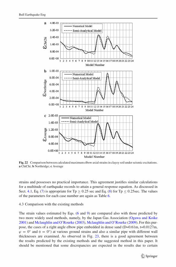
Fig. 21 Comparison between calculated maximum elbow axial strains in sandy soil under seismic excitations,a ChiChi; b Northridge; c Average
εChiChi = 2.44 × 10⁻⁵
(
−4.84
(θ
θS
)2
+ 6.61θ
θS
)7.34 (Vs
VS−Bedrock
)0.22 (PG A
g
) (D
t
)−0.3
(7)
εNorthridge = 1 × 10⁻⁷
(
−3.33
(θ
θS
)2
+ 5.12θ
θS
)14.25 (Vs
VS−Bedrock
)0.3 (PG A
g
)0.3 (D
t
)−0.11
(8)
εAverage = 2.7 × 10⁻⁴
(
−3.02
(θ
θS
)2
+ 4.28θ
θS
)7.4 (Vs
VS−Bedrock
)0.2 (PG A
g
)0.6 (D
t
)−0.3
(9)
Again, the above equations are illustrated for the different cases calculated in Fig. 22, showinggenerally a very good agreement. While for the governing majority of cases the relativedifference between the average numerical and semi-analytical predictions of Fig. 22 is lessthan 5 %, a larger difference is observed only for the case of pipe buried in soft clay with anelbow angle of 90 deg., and D/t=85 (model No. 12). Again, this case corresponds to very small
123
Bull Earthquake Eng
Fig. 22 Comparison between calculated maximum elbow axial strains in clayey soil under seismic excitations.a ChiChi; b Northridge; c Average
strains and possesses no practical importance. This agreement justifies similar calculationsfor a multitude of earthquake records to attain a general response equation. As discussed inSect. 4.1, Eq. (7) is appropriate for Tp ≥ 0.25 sec and Eq. (8) for Tp ≤ 0.25sec. The valuesof the parameters for each case number are again as Table 6.
4.3 Comparison with the existing methods
The strain values estimated by Eqs. (6 and 9) are compared also with those predicted bytwo more widely used methods, namely, by the Japan Gas Association (Ogawa and Koike2001) and Mclaughlin and O’Rourke (2003), Mclaughlin and O’Rourke (2009). For this pur-pose, the cases of a right angle elbow pipe embedded in dense sand (D=0.61m, t=0.0127m,ϕ = 0◦ and θ = 0◦) at various ground strains and also a similar pipe with different wallthicknesses are examined. As observed in Fig. 23, there is a good agreement betweenthe results predicted by the existing methods and the suggested method in this paper. Itshould be mentioned that some discrepancies are expected in the results due to certain
123
Bull Earthquake Eng
Fig. 23 Comparison between results predicted by the semi-analytical method and the two widely used meth-ods; for the case of a pipe buried in dense sand under various ground strains and wall thicknesses (H=0.91 m,D=61 cm, t=12.7 mm, Elbow angle=90 deg, θ = 0◦, ϕ = 0◦). Comparison with the: a approaches separately, baverage of the approaches, c approaches separately, ground strain=0.001, d average of the approaches, groundstrain=0.001, e approaches separately, ground strain=0.002, f average of the approaches, ground strain=0.002
differences in the assumptions. For instance, in the Ogawa and Koike (2001) method, asurface layer resting on half-space is considered, and this affects the pipe response consid-erably. There is an increase in ground strains in shallow depths and pipe strains as well,for a soft layer over a relatively rigid halfspace. Moreover, in the current paper‘s approach,the analyses were three dimensional in comparison with other mentioned methods that are2D. So, effect of the third component of earthquake ground motion records could lead tocertain changes in the pipe response. It is also worth mentioning that in quasi-static analysisused by the aforesaid approaches, one type of waves, usually Rayleigh waves, is consid-ered as the seismic wave, whereas in the time history analysis the pipe is subjected to acombination of different wave types with various wave lengths and propagation veloci-ties. Nevertheless, in spite of all the differing factors, there is still a very good agreementbetween the results predicted by the proposed regression equations in the present study andthe widely used methods in the literature. It is noteworthy that while the effects of almostall important factors in buried pipes analysis such as geometrical parameters of the pipeelbow, soil type, and the seismic loading are considered in the suggested equations, they
123
Bull Earthquake Eng
Table 7 The ratio of max.principal strain in hybrid model tomax. axial strain in beam model
Earthquake Soil type
Loose sand Medium sand Dense sand
Chichi 1.52 1.48 1.22
Northridge 1.54 1.03 1.01
Average 1.52 1.39 1.18
Design factor 1.5 1.4 1.2
Soft clay Medium clay Stiff clay
Chichi 1.40 1.08 1.04
Northridge 1.29 1.20 1.15
Average 1.39 1.09 1.05
Design factor 1.4 1.1 1.1
are very simple and fast to use and do not need complex and time consuming mathemati-cal calculations. Therefore, in comparison with other widely used methods, the suggestedformulation is able to predict the elbow pipe response with a reasonable accuracy at lowcost.
5 Design application of the semi-analytical model
Design of embedded pipes at bends under earthquake loading can be based on keeping theprincipal strain at that location below the yield level. Equations 6 and 9 prepare an approximateyet accurate enough tool for this purpose. On the other hand, before being suitable for designapplications, the value derived from the above equations must be converted to the principalstrain. The later quantity can be considerably larger than the maximum axial strain since thevalue of the hoop strain is also large at the bend. As described in the previous sections, whilethe bulk of analysis was based on the beam model unable to determine the hoop strain, thesame strain was calculated for a number of cases using a hybrid shell model. The cases includeseismic waves propagating parallel to a leg of the 90-degree bend. Therefore, it is possibleto calculate a conversion factor, as the ratio of the principal to the axial strains, for thosecases. Table 7 provides the conversion factors for different soils, the two earthquakes, andtheir averages. It should be noted that the average factors are ratios of the average principalstrains to the average maximum axial strains of the two earthquakes, not the averages of theconversion factors.
The conversion factor varies between 1.2 and 1.5 for dense to loose sand and 1.1 and 1.4for stiff to soft clay. Since this is not a large ratio, it can be concluded that the axial strainhas an essential contribution to the principal strain. On the other hand, the conversion factordoes not vary considerably for very different soils and two different earthquakes. Therefore,for design purposes, it can be taken as a constant value, to the safe side, for sand or forclay or even for both, equal to 1.5. This is based on the above limited data with a consistenttrend.
6 Conclusions
In this study the response of a buried pipe with bend was evaluated. The conclusions are asfollows:
123
Bull Earthquake Eng
1. An important effect of bend is increasing axial strains at bend location in comparisonwith straight pipe.
2. Axial strain at bend is larger in stiffer soils due to smaller slippage.3. The assumption of vertical propagation of waves results in negligible strains in pipe, and
should be abandoned where justifiable, like in deep basins.4. Axial strain in bends attains its maximum values for horizontally propagating waves
parallel to a pipe branch.5. A bend angle in the vicinity of 135◦ results in the largest axial strains in most of the cases
studied compared to usual 90◦ bends. In some cases it even exceeds the yield limit but isstill well below rupture level.
6. While D/t is a definitive ratio for axial strain of bend, effect of the H/D ratio is smalland can be disregarded.
7. Overall, modeling pipes and bends with shell elements do not significantly increase theaccuracy of results for predicting pipe elbow axial strains in wave propagation analy-sis compared with the much simpler beam model. It is not recommended for practicalpurposes, except when accounting for local buckling or hoop strain.
8. A semi-analytical model which is based on regression analysis is developed. The resultsof regression equations are found to be in good agreement with exact numerical resultsfor pipe response. The suggested equations estimate the maximum axial strain of buriedpipes at the elbow under wave propagation with much less effort and time with regard tothe complex 3D numerical models.
9. A factor converting the maximum axial strain to the principal strain at bend is presented.It is shown that the variation of this factor for very different cases is limited to 1.1–1.5.It is suggested that this factor is taken as equal to 1.5 for design purposes.
References
American lifelines alliance (ALA) (2001) Guidelines for the design of buried steel pipe (with addenda through2005). American Society of Civil Engineers
American Petroleum Institute (2000) Specificarion for line pipe. API specification 5L, Forty-Second EditionAmerican Society of Civil Engineers (1984) Guidelines for the seismic design of oil and gas pipeline systems.
Committee on Gas and Liquid Fuel Lifelines Technical Council on Lifeline Earthquake Engineering, NewYork
Berrones RF, Liu XL (2003) Seismic vulnerability of buried pipelines. Geofisica Internacional 42(2):237–246Bowles JE (1996) Foundation analysis and design. The McGraw-Hill Companies, NYChopra AK (1995) Dynamics of structures: theory and application to earthquake engineering. Prentice-Hall,
Englewood CliffsDash SR, Jain SK (2008) An overview of the seismic considerations of buried pipeline. J Struct Eng 34(5):
349–359Datta TK (1999) Seismic response of buried pipelines: a state-of-the-art review. Nucl Eng Des 192:271–284Goodling EC (1983) Buried piping—an analysis procedure update. In: Proceedings international symposium
on lifeline earthquake engineering, Portland, Oregon, ASME, PVP-77: 225–237Halabian AM, Hokmabadi T, Hashemolhosseini SH (2008) Numerical study on soil-HDPE pipeline interaction
subjected to permanent ground deformation. The 14th world conference on earthquake engineering, Beijing,China
Hart JD, Zulfiqar N, Lee CH, Dauby F, Kelson KI, Hitchcock C (2004) A unique pipeline fault crossing designfor a highly focused fault. In: Proceedings of IPC, international pipeline conference, Calgary, Alberta,Canada
Hatzigeorgiou GD, Beskos DE (2010) Soil-structure interaction effects on seismic inelastic analysis of 3-Dtunnels. Soil Dyn Earthq Eng 30:851–861
Hindy A, Novak M (1979) Earthquake response of underground pipelines. Earthq Eng Struct Dyn 7:451–476Horikawa H, Suzuki N (2009) Bending deformation of x80 cold bend pipe. In: Proceedings of the nineteenth
international offshore and polar engineering conference, Osaka, Japan
123
Bull Earthquake Eng
Japan Gas Association (JGA) (2000) Seismic design guideline of high-pressure gas pipelines. Japan GasAssociation
Karamanos SA, Giakoumatos E, Gresnigt AM (2003) Nonlinear response and failure of steel elbows underin-plane bending and pressure. J Press Vessel Technol 125(4):393–402
Karamanos SA, Tsouvalas D, Gresnigt AM (2006) Ultimate bending capacity and buckling of pressurized 90deg steel elbows. J Press Vessel Technol 128(3):348–356
Kishida H, Takano A (1970) The damping in the dry sand. The proceeding of 3rd Japan earthquake engineeringsimposium, Tokyo, Japan
Kouretzis GP, Bouckovalas GD, Gantes CJ (2006) 3-D shell analysis of cylindrical underground structuresunder seismic shear (S) wave action. Soil Dyn Earthq Eng 26:909–921
Kouretzis GP, Bouckovalas GD, Gantes CJ (2007) Analytical calculation of blast-induced strains to buriedpipelines. Int J Impact Eng 34:1683–1704
Lee DH, Kim BH, Lee H, Kong JS (2009) Seismic behavior of a buried gas pipeline under earthquakeexcitations. Eng Struct 3:1011–1023
Liu AI, Hu YX, Zhao FX, Li XJ, Takada S, Zhao L (2004) An equivalent-boundary method for the shellanalysis of buried pipelines under fault movement. Acta Seismol Sinica 17:150–156
Lysmer J, Kuhlemeyer AM (1969) Finite dynamic model for infinite media. J Eng Mech Div 95(4):859–877Mclaughlin PM, O’Rourke M (2003) Seismic response and behavior of buried continuous piping systems
containing elbows. Doctoral Thesis, Rensselaer Polytechnic InstituteMclaughlin PM, O’Rourke M (2009) Strain in pipe elbows due to wave propagation hazard. Lifeline Earthquake
Engineering in a Multihazard Environment, ASCEMuthmann E, Grimpe F (2006) Fabrication of hot induction bends from LSAW large diameter pipes manufac-
tured from TMCP plate. Microalloyed steels for the oil and gas industry international symposium, Araxa,Brazil
Newmark NM (1968) Problems in wave propagation in soil and rock. In: Proceedings of international sympo-sium on wave propagation and dynamic properties of earth materials, August 23–25, Univ. of New MexicoPress, Albuquerque: 7–26
Ogawa Y, Koike T (2001) Structural design of buried pipline for sever earthquake. Soil Dyn Earthq Eng21:199–209
O’Rourke MJ, Liu X (1999) Response of buried pipelines subject to earthquake effects. MCEER MonographSeries, Multidisciplinary Center for Earthquake Engineering Research
O’Rourke TD, Wang Y, Shi P, Jones S (2004) Seismic wave effects on water trunk and transmission lines.In: Proceedings of the 11th international conference on soil dynamics and earthquake engineering and 3rdinternational conference on earthquake geotechnical engineering. Berkeley, CA 2:420-428
O’Rourke MJ, El Hmadi K (1988) Analysis of continuous buried pipelines for seismic wave effects. EarthqEng Struct Dyn 16:917–929
Pacific Earthquake Engineering Research Center, http://peer.berkeley.edu/, PEERPappa P, Tsouvalas D, Karamanos SA, Houliara S (2008) Bending behavior of pressurized induction bends.
Offshore Mechanics and Arctic Engineering Conference, ASME, OMAE2008-57358, Lisbon, PortugalRofooei FR, Qorbani R (2008) A parametric study on seismic behavior of continuous buried pipeline due to
wave propagation. The 14th world conference on earthquake engineering, Beijing, ChinaSakurai A, Takahashi T (1969) Dynamic stresses of undergroud pipelines during earthquake. In: Proceeding
of the fourth wolrd confrenece on earthquake engineering, Santiago, Chile, pp 81–95Shah H, Chu S (1974) Seismic analysis of underground structural element. J Power Div 100:53–62Shi P, O’Rourke TD, Wang Y, Fan K (2008) Seismic response of buried pipelines to surface wave propagation
effects. The 14th world conference on earthquake engineering. Beijing, ChinaStamos AA, Beskos DE (1995) Dynamic analysis of large 3-D underground structures by the BEM. Earthq
Eng Struct Dyn 24:917–934Takada S, Tanabe K (1987) Three dimensional seismic response analysis of buried continuous or jointed
pipelines. J Press Vessel Technol 109:80–87Takada S, Hassani N, Fukuda K (2001) A new proposal for simplified design of buried steel pipes crossing
active faults. Earthq Eng Struct Dyn 30:1243–1257Takada S, Carlo A, Bo S, Wuhu X (1992) Current state of the arts on pipeline earthquake engineering in japan.
The construction engineering research institute foundation: 305–326Takada S, Higashi S (1992) Seismic response analysis for jointed buried pipline by using shell FEM model.
In: Proceedings of the tenth world conference on earthquake engineering pp 5487–5492Takada S, Katagiri S (1995) Shell model response analysis of buried piplines. In: Proceedings of the fourth
U.S. confrence of lifeline earthquake engineering , pp 256–263Trifonov OV, Cherniy VP (2010) A semi-analytical approach to a nonlinear stress-strain analysis of buried
steel pipelines crossing active faults. Soil Dyn Earthq Eng 30:1298–1308
Vazouras P, Karamanos SA, Dakoulas P (2010) Finite element analysis of buried steel pipelines under strike-slip fault displacements. Soil Dyn Earthq Eng 30:1361–1376
Wang Y, O’Rourke TD, Shi P (2006) Seismic wave effects on the longitudinal forces and pullout of undergroundlifelines. In: Proceedings of the 100th anniversary earthquake conference: commemorating the 1906 SanFrancisco Earthquake, San Francisco, California, Aplil 18–22
Yoshizaki K, O’Rourke TD, Hamada M (2001) Large diformation behavior of buried pipeline with low angleelbows subjected to permanent ground deformation. Proc JSCE (Japan Society of Civil Engineers) 675:41–52