195

Available at

http://pvamu.edu/aam Appl. Appl. Math.

ISSN: 1932-9466

Vol. 10, Issue 1 (June 2015), pp. 195 - 211

Applications and Applied

Mathematics:

An International Journal

(AAM)

A Semi-parametric Approach for Analyzing Longitudinal Measurements with

Non-ignorable Missingness Using Regression Spline

Taban Baghfalaki*

Department of Statistics

Tarbiat Modares University

Tehran, Iran

t.baghfalaki@modares.ac.ir

Saeide Sefidi and Mojtaba Ganjali Department of Statistics

Shahid Beheshti University

Tehran, Iran *Correspondence author

Received: April 24, 2014; Accepted: February 2, 2015

Abstract In longitudinal studies with missingness, shared parameter models (SPM) provide appropriate

framework for the joint modeling of the measurements and missingness process. These models use a

set of random effects to account for the interdependence between two processes. Sometimes the

longitudinal responses may not be fitted well by using a linear model and some non-parametric

methods have to be used. Also, parametric assumptions are typically made for the random effects

distribution, and violation of those may affect the parameter estimates and standard errors. To

overcome these problems, we propose a semi-parametric model for the joint modelling of

longitudinal markers and a missing not at random mechanism. In this model, because of the

flexibility in nonparametric regression models, the relationship between the response variables and

the covariates has been modeled by semi-parametric mixed effect model. Also, we do not assume any

parametric assumption for the random effects distribution and we allow it to be unspecified. The

parameter estimations are made using a vertex exchange method. In order to evaluate the

performance of the proposed model, we compare SPM using regression spline (Spline-SPM) and

semi-parametric SPM (SpSPM) models. We also conduct a simulation study with different

parametric assumptions for the random effects distribution. A real example from a recent HIV study

is analyzed for illustration of the proposed approach.

Keywords: Joint modeling; Longitudinal data; Missing mechanism; Nonparametric model;

Regression spline; Random effects; Vertex exchange method.

MSC 2010 No.: 62J02, 62H12

196 Taban Baghfalaki et a1.

1. Introduction

In longitudinal studies, individuals are followed over a duration of time and for each individual,

data are collected at multiple time points. These repeated measurements may share a common

characteristic and may be correlated, although measurements on different individuals could be

assumed to be independent. Consideration of correlations within measurements of the same

individual expresses the key characteristic of longitudinal data.

Missingness is a problem of longitudinal data. In some cases, a subject may be missing in one or

several measurement occasions. Rubin (1976) provided a framework for the incomplete data by

introducing the important classification of missing data mechanisms, which consist of missing

completely at random (MCAR), missing at random (MAR) and missing not at random (MNAR).

A mechanisms is called MCAR if the missing mechanism is independent of the unobserved and

also observed data, MAR if, conditional on the observed data, the missing mechanism is

independent of the missing measurements; otherwise the missing process is termed MNAR. As

an example of MNAR, a patient decides not to show up at some of the scheduled visits because

of her/his very bad current health conditions. The missingness depends on unobserved responses.

In such cases, analyzing the longitudinal measurements for disease evaluations using, e.g., a

mixed effects model, where ignoring the missingness process, leads to biased inferences.

For the joint modeling of these two processes, Shared Parameter Model (SPM) (Wu and Carroll,

1988; Follmann and Wu, 1995) can be used. In this approach, the two models are linked through

some common unknown variables. Shared parameter models suppose that a set of random effects

induce the interdependence. In particular, consider the vector Y as a complete longitudinal

response and based on the missingness process, R divide it into two parts of oY and

mY which

are the observed and missing components, respectively. Under the SPM framework, the joint

density of the measurement process Y and the missingness process R may be completed as

,)|(),|(),|,(=)|,,( dbbfbRfbYYfRYYf bRY

momo

(1)

where (.)f denotes a probability density function, b is a vector of random effects, and '

b'

R'

Y' ),,(= . In , Y is the parameter vector of the model for Y given b , R is the

vector of parameters of R given b and b is the vector of parameters of the distribution of

.b This factorization shows that given the random effect b , the vector of response variable )(Y

and missingness process )(R are independent. According to De Gruttola and Tu (1994) and

Little (1995) , SPMs are appropriate when missingness is due to an underlying process by which

the longitudinal responses are measured with error. The size of this measurement error

determines the strength of the dependence of the missingness on the latent variable b . The

construction of an SPM missingness mechanism leads to a missing not at random (Rubin, 1976)

process, where the missing data mechanism (1) is given by

,),,|(),|(=),,|( bdYYbfbRfYYRf b

mo

R

mo (2)

AAM: Intern. J., Vol. 10, Issue 1 (June 2015) 197

which shows that the probability of nonresponse depends on ),,|( b

mo YYbf . Therefore, the

random effects are the main component in the modeling of the missing data. However,

misspecification for distribution of random effects can severely affect our inference. Finding

suitable parametric distribution assumption for the random effects is however difficult.

Because, the potential dependence of the random effects on unobserved covariates induces

heterogeneity that cannot be captured by common parametric assumptions (Tsonaka et al., 2009).

Several authors have proposed joint models that are not dependent on strong parametric

assumptions for the random effects, and are also robust to some distributional assumptions. In

particular, in the context of joint modeling of longitudinal measurements and survival data, Song

et al. (2002) have given a shared latent component which is the product of a polynomial term and

the standard normal density. In missing data analysis, Lin et al. (2000) and Beunckens et al.

(2008) assume that the random effects have a finite mixture of normal distribution. Also they

offer some insight in the shape of the random effects distribution, which helps in determining a

potential subpopulation structure in the data, and produces enhanced subject-specific predictions.

In this paper, we propose to leave the random effects distribution completely unspecified. The

estimation of this model is based on a semi-parametric method that assumes the random effects

distribution to be discrete with unknown support sizes. To effectively maximize the log-

likelihood with respect to the random effects distribution, we apply the Vertex Exchange Method

(VEM) (Bohning, 1985). For longitudinal data, parametric mixed-effects models, such as linear

and nonlinear mixed-effects models are a natural tool. Linear mixed-effects (LME) models are

used when the relationship between a longitudinal response variable and its covariates can be

expressed via a linear model. Nonlinear mixed-effects (NLME) models are used when the

relationship between a longitudinal response variable and its covariates cannot be expressed via a

linear model.

A parametric regression model requires an assumption that the form of the underlying regression

function is known except for the values of a finite number of parameters. A disadvantage of

parametric modeling is that a parametric model may be too restrictive in some applications. The

use of an inappropriate parametric model leads to misleading results. For such a longitudinal data

set, we do not assume a parametric model for the relationship between the response variable and

the time as a covariate. Instead, we just assume that the individual and the population mean

functions are smooth functions of time t , and let the data themselves determined the form of the

underlying function.

There are many nonparametric regression and smoothing method. The most popular methods,

theincline kernel smoothing, local polynomial fitting, regression spline, smoothing spline and

penalized splines (Zhang et al., 1998; Wu and Zhang, 2002). Tsonaka et al. (2009) use LME

model for measurements process, called the SpSP model (semi-parametric shared parameter

model). But, the process that the data are generated from (such as our data) may not be linear,

thus for analyzing this kind of data set, the LME model is inapplicable. Therefore, for

measurements process the modeling we use is the regression spline for nonparametric fixed-

effects component of the semi-parametric model. We called it the Spline-SpSP model (semi-

parametric shared random effects model using regression spline). Also, the VEM is used for joint

modeling of the missingness process and longitudinal measurements.

198 Taban Baghfalaki et a1.

The paper is organized as follows: the nonparametric regression for longitudinal data is

considered in Section 2. Section 3 presents the proposed modeling framework. Also, this Section

summarizes some theoretical results and gives the details for the estimation procedure. The

performance of the proposed method is evaluated via some simulation studies in Section 4. The

proposed approach is applied for analyzing a real data set in Section 5. The final section includes

some concluding remarks.

2. Semi-parametric mixed-effects model

The parametric models are usually restrictive and less robust against modification of model

assumption, but they are advantageous and efficient when models are correctly specified. In

contrast, nonparametric models are more robust against the model assumption than a parametric

model, but they are usually more complex and less efficient. Semi-parametric models are

performs well and retain nice features of both parametric and nonparametric models. In semi-

parametric models the parametric components are often used to model important factors that

affect the responses parametrically and the nonparametric components are often used for

nuisance factors which are usually less important (Wu and Zhang, 2004).

2.1. Models specification

A longitudinal data set can be expressed in a common form as

,, ... 1,2,= ,, ... 1,2,=),,( iijij njniyt

(3)

where ijt denotes designsated time points, ijy the observed response at time ijt , in the number of

observations for the i th subject and n is the number of subjects. In the semi-parametric mixed-

effects model (SpME), the mean response function at time ijt depends on time ijt

nonparametrically via a smooth function )(t , and linearly on some other observable covariates '

ijpijij ccc ),...,(=0

1 , where 0p is the number of covariates observed at time ijt . The random effect

components at time ijt may depend on time ijt nonparametrically via a smooth process (.)i and

linearly on some other covariates, namely ,),...,(=0

1

'

ijqijij hhh where 00 pq . The resulting

model may be written as

,, ... 1,=,, ... 1,=,)()(= ninjtbhtcy iijijiiij

'

ij

'

ijij (4)

where and (.) are smooth functions of time, '

iqii bbb ),...,(=0

1 consists of the coefficients of

the covariate vector ijh , )(ti is smooth process of time, and ij is the error at time ijt that is not

explained by either the fixed-effects component )( ij

'

ij tc or the random effects component

)( ijii

'

ij tbh . Other special SpME models are obtained when one or two SpME components are

dropped from the general SpME model (4). When only the nonparametric random-effects

AAM: Intern. J., Vol. 10, Issue 1 (June 2015) 199

component is dropped, the SpME model (4) reduces to the following SpME model

., ... 1,=;, ... 1,=,)(= ninjbhtcy iiji

'

ijij

'

ijij (5)

Ruppert et al. (2003) dealt with a simple version (with 1=0q ) of this type of SpME model

using penalized splines.

For the longitudinal responses iY , the SpME model can be written as

,= iiiiii bHCY (6)

where '

iiniii yyyY ), ... ,,(= 21 , '

iiniii ttt ))(, ... ),(),((= 21 ,

'

iiniii cccC ), ... ,,(= 21 , '

iiniii hhhH ), ... ,,(= 21 and )(0, ii N .

The error terms i are assumed independent of ib and i

ni I2= . We can approximately

express )(t as a regression spline. In regression spline smoothing, local neighborhoods are

specified by a group of locations, say, 110 ,, ... ,, KK in the range of interest, such that, an

interval ],[ ba can be considered as:

.=<< ... <<= 110 ba KK

(7)

These locations are known as knots; and Krr , ... 1,2,= , are called interior knots or simply

knots. A regression spline can be constructed using the following so called k th degree truncated

power basis with K knots K , ... ,, 21

,))(, ... ,)(,, ... ,(1,=)( 1

'k

K

kk

p ttttt

(8)

where k is chosen 2 or 3 and kk aa )(= denotes power k of the positive part of a ,

)(0,= amaxa and 1= kKp denotes the number of the basis functions involve which are

called smoothing parameters. We can express ,)()( '

p tt where '

p ), ... ,(= 1 is the

associated coefficients vector. For locating the knots, we can use equally spaced sample

quantiles as knots. Let Mlt l , ... 1,2,=,)( be the order statistics of the pooled design time points,

where

i

n

i

nM 1=

= .

Then the K knots are defined as

200 Taban Baghfalaki et a1.

,1,...,=,= 1)])/([(1 Krt KrMr

(9)

where ][a denotes the integer part of a . For smoothing parameter selection, a good selector

usually tries to select a good smoothing parameter p to trade-off the goodness of fit of the

smoother and its model complexity. Generalized cross-validation (GCV) is a smoothing

parameter selector which is defined as follows

.)/)/(1ˆ()ˆ(=)( 2

1=

MpyyyypGCV ii

T

ii

n

i

(10)

Notice that the numerator in the GCV score, is the SSE (sum of squared errors), representing the

goodness of fit, and denominator is associated with the model complexity, where p is the model

complexity in regression spline.

2.2. Specification of missingness model

Consider a general pattern of missing data and let R be the associated matrix of the missingness

indicator related to the Y matrix and 1=ijR if ijY is observed and otherwise 0=ijR . For the

missingness process R , probability of response, )|1=(= iijij bRPrp , is modeled using a mixed

effects logistic regression model as follows:

,=)( i

'

ij

'

ijij bzwplogit (11)

where '

ijw is the j th row of the fixed effects design matrix iW , the regression coefficient

vector, '

ijz the j th row of iZ , and )(= diag . As above, covariates in iZ are not included in

iW . The measurements and missingness processes are linked through the random effects term

and their association is quantified by the parameter vector .

3. Random effects estimate

In this paper we make no parametric assumptions for the random effects distribution and leave it

completely unspecified. We assume that Gbi , with MG , where M is the set of all

distribution functions on the parameter space M of ib (Tsonaka et al., 2009). Thus marginal

density for iY and iR is given by:

).(),|(),|(=),|,( iRiiiYim

ii bdGbRfbYfGRYf (12)

In general, G can be a discrete or a continuous distribution. However, Laird (1978) and

Lindsay (1983) have shown that the nonparametric maximum likelihood estimate )(NPMLE of

AAM: Intern. J., Vol. 10, Issue 1 (June 2015) 201

the unknown G is discrete with finite support and thus M reduces to includes all discrete

distributions. So, (12) would be

),,|(),|(=),|,( RciYcic

c

ii RfYfGRYf (13)

where ),(= RY includes the parameter vector for the Y and for all R processes,

,...),(= 21 is the support points and ,...),(= 21 is the corresponding weights of G . We

call the model defined by equation (13) Spline semi-parametric shared parameter model (Spline-

SpSP). This is due to having parametric assumptions for the involved submodels, but we have

the random effects distribution unspecified.

3.1. Estimation Procedure

A two-step procedure has been developed that is iterated until convergence. In the first step, G

is estimated for fixed at its current estimate and in a second step is updated by

maximizing the profile likelihood )ˆ|( Gl , where G denote the estimated G of the first step.

The latter step can be easily implemented using an optimization method of R software. Estimate

of G can be obtained using a VEM algorithm. The VEM is a directional derivative-based

algorithm that iteratively maximizes the log-likelihood )|( Gl in the set M of all discrete

distributions over a prespecified grid ), ... ,,( 21 C with C large.

The main idea of VEM is to search in each iteration for the direction that maximizes the log-

likelihood increase )()(= 01 GlGl (where 0G and 1G denote the current and updated

estimates of G , respectively), and exchange weights between the grid points that contribute the

least and the most to . These points are identified based on the properties of the directional

derivative of the log-likelihood from one distribution 0G to another 1G . When

1G is degenerate

at Ccc , ... 1,=, , then .=1c

GG In particular, the directional derivative ),( 0

cGGD

of )(Gl at

0G in the direction of c

G is defined as

.

)())((1lim=),(

00

0

0

s

GlsGGslGGD

c

sc

(14)

For each grid point c , with Cc , ... 1,= , we evaluate the directional derivative, for fixed )(ˆ it , in

the case of the proposed Spline-SpSP model takes the form

,)ˆ,|,(

)ˆ,|,(=),(

01=

0 nGRYf

GRYfGGD

ii

cii

n

ic

(15)

for proof, let

),ˆ,|,(log=)ˆ,|,(log=)(1=1=

GRYfGRYfGl ii

n

i

ii

n

i

(16)

202 Taban Baghfalaki et a1.

We use (14) and (16) for ),( 0

cGGD , so that

0 0

0 =1

0

=1

1 ˆ ˆ( , ) = log [(1 ) ( , | , ) ( , | , )]lim

ˆlog ( , | , )

n

i i i ic cs i

n

i i

i

D G G s f Y R G sf Y R Gs

f Y R G

0

00 =1

ˆ ˆ(1 ) ( , | , ) ( , | , )1= log .lim ˆ( , | , ),

ni i i i

c

s i i i

s f Y R G sf Y R G

s f Y R G

(17)

Using the L’hopital rule, equation (17) lead to (15). Also, we have

0

=1

ˆ ˆˆ( , | , ) = ( , | , ).C

i i c i i c

c

f Y R G f Y R (18)

So equation (18), for the each iteration, can be written as

.

)ˆ,|,(ˆ

)ˆ,|,(=),ˆ(

)(

1=

1=

n

RYf

RYfGGD

it

cii

it

c

C

c

it

ciin

ic

it

(19)

As a first step, we specify the grid c . ib is a q dimensional vector. Thus a grid for ib defined

in [ , ] = [ , ] [ , ]q with of order 4 or 5 would in most cases be sufficient. For

each c , with Cc , ... 1,= , we get a q variate vector, where components must be chosen in

4,4][U , such that kcc )/2( 1 , with 0.1=k . Then, (19) is computed for all c s. Note that

initial value for the parameters ),( 00

RY of the Y and R processes, can be obtained by fitting the

appropriate ignorable mixed effects models, i.e., a linear mixed model and a mixed effects

logistic regression, respectively. Initial values for the corresponding weights of the support

points c are C1/ . After specifying all directional derivatives, and as follows

),,ˆ(maxarg=),,ˆ(minarg=

GGDGGD it

c

it

c

(20)

and their weights updated according to

,ˆˆ=ˆ,ˆ)(1=ˆ )()(*1)()(*1)( ititititit ss

(21)

where [0,1])( * s denote the step length defined as

AAM: Intern. J., Vol. 10, Issue 1 (June 2015) 203

}].ˆ|ˆ{}ˆ|)(ˆ{[maxarg= 1* itititit

s

GlsGls (22)

The estimation of *s is implemented using a line search method.

Note that if 1=*s then 0=ˆ

and thus is excluded from the grid and the grid size reduce

to 1C .

After estimating 1)(ˆ itG in the first step, in the second step by using for example “optim" function

in the R software, the vector is estimated. These two steps are repeated iteratively until

convergence. The algorithm converges when the following conditions are satisfied

<),ˆ(max)( GGD it

which guarantees that <)ˆ|ˆ()ˆ|ˆ( 1)(1)(1)()( itititit GlGl .

Note that the submodels (6) and (11) require the mean of the random effects to be zero, i.e.,

cc

C

c

ibE 1=

=)( .

To ensure identifiability, we fix through the optimization procedure that the models intercepts

follow

.ˆ=,ˆ=1=

00

1=

00 cc

C

c

bnewcc

C

c

bnew SS (23)

4. Simulation study

A simulation study is implemented to investigate the performance of the proposed method. The

performance of our model is evaluated with the use of various distributional assumptions for the

random effects component. We compare the Spline-SpSP model with two other models. The first

model is Spline-SPM, where the longitudinal process is modeled with the spline and the second

model is the SpSPM, where the longitudinal process is modeled by a linear model. We show

robustness of the Spline-SpSP model with respect to distribution assumptions of the random

effects and nonlinearity of the model. The longitudinal process Y is simulated from the following

semi-parametric model:

,)()(= 5

2

24

2

13

2

210 ijiiijijijijij bttttY (24)

where the subscripts ni 1,...,= denotes the subject, and N1,...,=j denotes the repeated

measurements, where i

i

nmax=N , ijt is the time variable that takes values in [0,3] , i is the

binary covariate and ib is the random effects component. The parameter vector is taken as

2.5=0 , 2=1 , 0.4=2 , 1.8=3 , 2=4 and 1.5=5 . For the error component, we

assume )(0, 2

Yij N with 0.5=2

Y . Two sample sizes 200=n and 500=n with 5=N

equally spaced visit times is assumed.

204 Taban Baghfalaki et a1.

A model that set is for R process is the non-monotone missingness model. The binary indicator

ijR is simulated from a mixed effects logistic regression

,=)|1=( 210 iijiiij btbRlogitP

where 1.1=0 , 2=1 and 0.5.=2 Using this logistic model, we generate a matrix

containing zero and one. This matrix is called the missingness matrix. The ijY that corresponds to

the zero elements of the matrix go to be missing values in the data set.

The assumed values for the regression parameters are chosen such that they lead to

approximately 20% of the missing. The shared random intercepts ib linked the Y and R

processes, also we assume 2.5= . For random effect ib three scenarios are considered: a

distribution (0,2)N , a mixture of two normal components, )(1.35,0.20.5)1.35,0.6(0.5 22 NN ,

a discrete distribution with support at 1.7575,0.5,0.5,1. and corresponding weights 0.32 ,

0.18 , 0.18 and 0.32 . For each of these three scenarios 200 and 500 samples are simulated.

Each sample was fitted under Spline-SpSP, Spline-SP and SpSP models. The SpSP model which

is used for analyzing the generated data set is:

.= 510 ijiiijij btY (25)

Comparisons between estimates are based on the root mean squared error (RMSE) and relative

biases (RB) which are defined as:

1).ˆ

(1

=)(,)ˆ(1

=)(

*

1=*

2

*

1=*

i

N

i

i

N

i NRB

NRMSE

The results of this simulation are presented in Tables 1 and 2. These simulation studies show that

the Spline-SpSP model is robust to the violation of distributional assumptions of the random

effects. When the random effects distribution is normal, parameter estimates of Spline-SpSP and

Spline-SP models are similar. But when the random effects distribution departs from normality

assumption, difference of the two models are unfolded and the Spline-SpSP model gives

parameter estimates that are closer to real values than parameter estimates in Spline-SP and SpSP

models. Moreover, the RMSE and RB of Spline-SpSP model is lower than Spline-SP and SpSP

models. Also it can be seen in Figure A.1 that our approach offers an informative insight on the

assumed shape of the random effects distribution.

5. Application

We apply the Spline-SpSP, Spline-SP and SpSP models to the analysis of the HIV-1 RNA data

(Sun and Wu, 2005 and Hammer et al., 2002) from an AIDS clinical trial study for comparing a

single protease inhibitor (PI) versus a double-PI antiretroviral regimens in treating HIV-infected

patients. In this study, all subjects start the antiretroviral treatment at time 0 and HIV-1 RNA

AAM: Intern. J., Vol. 10, Issue 1 (June 2015) 205

levels in plasma (viral load) was measured repeatedly over time. The scheduled visits for the

measurements were at weeks 0, 2, 4, 8, 16 and 24. A total of 481 patients were entered in the

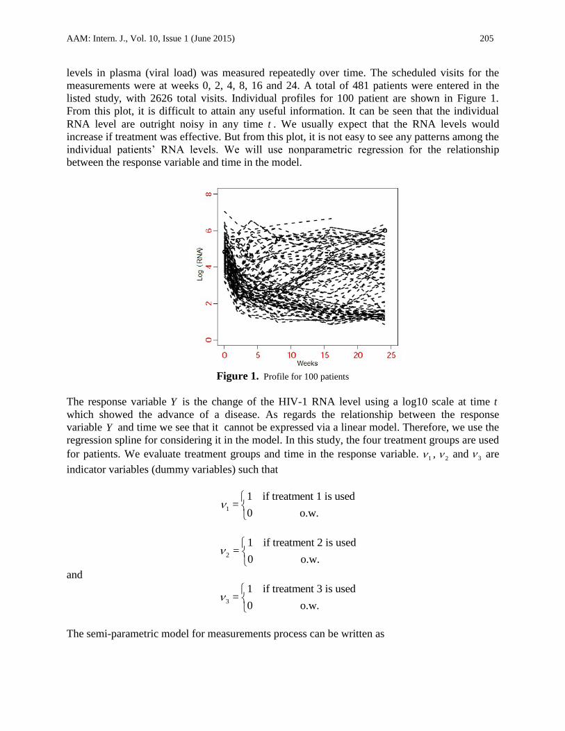
listed study, with 2626 total visits. Individual profiles for 100 patient are shown in Figure 1.

From this plot, it is difficult to attain any useful information. It can be seen that the individual

RNA level are outright noisy in any time t . We usually expect that the RNA levels would

increase if treatment was effective. But from this plot, it is not easy to see any patterns among the

individual patients’ RNA levels. We will use nonparametric regression for the relationship

between the response variable and time in the model.

Figure 1. Profile for 100 patients

The response variable Y is the change of the HIV-1 RNA level using a log10 scale at time t

which showed the advance of a disease. As regards the relationship between the response

variable Y and time we see that it cannot be expressed via a linear model. Therefore, we use the

regression spline for considering it in the model. In this study, the four treatment groups are used

for patients. We evaluate treatment groups and time in the response variable. 1 ,

2 and 3 are

indicator variables (dummy variables) such that

1

1 if treatment 1 is used=

0 o.w.

2

1 if treatment 2 is used=

0 o.w.

and

3

1 if treatment 3 is used=

0 o.w.

The semi-parametric model for measurements process can be written as

206 Taban Baghfalaki et a1.

,)()(= 372615

2

24

2

13

2

210 ijiiiiijijijijij btttty

where ,481...1,=i , inj ,...1,= and ,6...2,=in . We use the truncated power based on (8) with

2=k , and adopted the “equally spaced sample quantiles as knots" method to specify the knots.

Naturally, this model is jointed to the non-ignorable missingness model note that the percentage

of missingness is around 10% . The probability of response is modeled using a mixed effects

logistic regression as follows

.=))|1=(( 34231210 iiiiijiij btbrPrlogit (26)

The Y and R processes are linked through the shared random effect ib , and their association is

measured by the parameter . If 0= , the Y and R processes are independent. The estimated

parameters and their standard deviations (computed by the bootstrap method) are presented in

Table 3. These two models are compared by Akaike information criterion (Akaike 1973) and

Bayesian information criterion (Schwartz 1978). These are defined as

,)(2=,22= dfnlogLoglikBICdfLoglikAIC

where Loglik is the logarithm of the likelihood function and df is the model complexity which

is the number of basis function p together with 0p covariates observed at time t (Wu and

Zhang, 2004). It can be seen in Table 3 that AIC and BIC of the Spline-SpSP model is smaller

than those of the Spline-SP and SpSP models. The model produces reliable parameter estimates

under any distributional assumption for the random effects. Also according to Table 3, the

Spline-SpSP model shows that treatment 1 and treatment 2 are not significant. But, time is an

efficient variable; such that the more time, the less viral load measurements. Also, is a

significant parameter, i.e. missingness is found to be non-ignorable.

The fitted )(RNAlog for some randomly chosen subjects are presented in Figure A.2. To

summarize, these results suggest that the Spline-SpSP model provide precise prediction for the

dataset thanthe two other models.

6. Conclusion In this paper, we have focused on the use of a semi-parametric model in longitudinal data. At

first we explain shared parameter models as an appealing framework for the joint modeling of

the measurements and missingness processes, particulary in the nonmonotone missingness case.

We take a semi-parametric model for the measurment process and logistic regression as a model

for missingness mechanism. With the usage of a NPMLE method also called a vertex exchange

method, we estimate the random effect distribution. We use the Spline-SpSP model in some sets

of simulated data and considered the various distributional assumptions for the random effects.

Our study uses the Spline-SpSP model framework applying the nonmonoton non-ignorable

missingness. Our simulation studies show that the proposed model is robust to the various

distributional assumptions considered for the random effects. We also observed that the proposed

model produces estimates with RMSE and S.E. which are lower than those obtained by the

AAM: Intern. J., Vol. 10, Issue 1 (June 2015) 207

Spline-SP and SpSP models.

REFERENCES

Akaike, H. (1973). Information theory as an extension of the maximum likelihood principle.

Pages 267-281 in B. N. Petrov, and F. Csaki, (Eds.) Second International Symposium on

Information Theory. Akademiai Kiado, Budapest.

Beunckens, C., Molenberghs, G., Verbeke, G., and Mallinckrodt, C. (2008). A latent-class

mixture model for incomplete longitudinal Gaussian data. Biometrics, 64, 96-105.

Bohning, D. (1985). Numerical estimation of a probability measure. Journal of Statistical

Planning and Inference, 11, 57-69.

De Gruttola, V., and Tu, X. M. (1994). Modelling progression of CD-4 lymphocyte count and

its relationship to survival time. Biometrics, 50, 1003-1014.

Follmann, D., and Wu, M. (1995). An approximate generalized linear model with random

effects for informative missing data, Biometrics, 55, 151-168.

Hammer SM, Vaida F, Bennett KK et al. (2002). Dual vs single protease inhibitor therapy

following antiretroviral treatment failure: a randomized trial. JAMA, 288, 169-180.

Laird, N. (1978). Nonparametric maximum likelihood estimation of a mixing distribution.

Journal of the American Statistical Association, 73, 805-811.

Lin, H., Turnbull, B. W., McCulloch, C. E., Turnbull, B. W., Slate, E. H., and Clark, L. (2000).

A latent class mixed model for analysing biomarker trajectories with irregularly scheduled

observations. Statistics in Medecine, 19(10), 1303-1318.

Lindsay, B. G. (1983), The geometry of mixture likelihoods: A general theory. The Annals of

Statistics, 11, 86-94.

Little, R. (1995). Modeling the drop-out mechanism in repeated measures studies. Journal of

the American Statistical Association, 90, 438-450.

Rubin, D. B. (1976). Inference and missing data (with discussion). Biometrika, 63, 581-592.

Ruppert, D., Wand, M. P., and Carrol, R. j. (2003). Semi-parametric Regression, the press of

london Cambridge University.

Schwartz, G. (1978). Estimating the dimension of a model. Annals of statistics, 6, 461-464.

Song, X., Davidian, M., and Tsiatis, A. A. (2002). A semi-parametric likelihood approach to

joint modelling of longitudinal and time to event data. Biometrics, 58, 742-753.

Sun, Y. and Wu, H. (2005). Semiparametric Time-Varying Coefficients Regression Model for

Longitudinal Data, Scan. J. Statist., 32, 21-47.

Tsonaka, R., Verbeke, G., and Lesaffre, E. (2009). A Semi- Parameteric shared parameter

model to handle nonmonotone non-ignorable missingness. Biometerics, 65, 81-87.

Wu, M. C., and Carroll, R. (1988). Estimation and comparison of changes in the presence of

informative right censoring by modeling the censoring process. Biometrics, 44, 175-188.

Wu, H., and Zhang, J. T. (2002). Local polynomial mixed-effects models for longitudinal data

analysis. Journal of the American Statistical Association, 97, 883-897.

Wu, H., and Zhang, J. T. (2004). Nonparametric regression methods for longitudinal data

analysis. Wiley Series in Probability and Statistics, New York.

Zhang, D., Lin, X., Rez, J. and Sowers, M. (1998). Semiparametric stochastic mixed models for

longitudinal data. Journal of the American Statistical Association, 93, 710-719.

208 Taban Baghfalaki et a1.

Table 1. Results of the simulation study: Evaluation of the Spline-SpSP model and comparison with the Spline-SPM and SpSP models.

Mean (Est.), standard error (SE) and Root Mean Square Error (RMSE) for sample size 500 Spline-SpSP model Spline-SP model SpSP model

Par Real Est. S.E. RMSE RB Est. S.E RMSE RB Est. S.E. RMSE RB

Normal distribution

2.5 2.526 0.227 0.222 0.11 2.508 1.012 1.012 0.003 2.625 0.436 0.437 0.103

2.0 1.976 0.685 0.685 -0.012 2.114 0.254 0.255 0.207 1.646 0.639 0.641 0.048

-0.4 -0.383 0.039 0.036 -0.152 -0.447 0.123 0.127 0.163 - - - -

-1.8 -1.824 0.427 0.430 0.040 -1.814 0.541 0.562 -0.189 - - - -

2.0 2.021 0.328 0.321 0.024 1.971 0.525 0.525 -0.015 - - - -

1.5 1.503 0.054 0.053 -0.063 1.507 0.197 0.198 -0.015 1.272 0.213 0.214 -0.045

1.1 1.191 0.352 0.406 0.072 1.147 0.128 0.124 0.006 1.291 0.241 0.243 0.024

2.0 1.992 0.361 0.362 -0.039 2.020 0.014 0.013 0.002 1.745 0.125 0.129 0.043

0.5 0.501 0.121 0.126 0.001 0.497 0.164 0.161 -0.031 0.342 0.112 0.113 0.032

0.5 0.472 0.054 0.057 2.018 0.477 0.051 0.055 0.241 0.621 0.121 0.124 0.056

2.5 2.410 0.190 0.114 -0.231 2.564 0.541 0.543 -0.186 2.850 0.417 0.423 -0.074

2.0 2.006 0.394 0.397 -0.036 1.991 0.314 0.14 -0.071 1.891 0.328 0.329 0.012

Mixture of two normal distributions

2.5 2.503 0.644 0.644 0.001 2.625 0.704 0.712 0.034 2.738 0.504 0.506 -0.021

2.0 2.073 0.231 0.238 0.026 1.998 0.532 0.532 -0.002 2.243 0.692 0.695 0.031

-0.4 -0.404 0.129 0.122 0.304 -0.382 0.051 0.052 -0.036 - - - -

-1.8 -1.773 0.576 0.572 -0.048 -1.876 0.225 0.229 0.009 - - - -

2.0 2.003 0.04 0.043 0.001 2.101 0.241 0.249 0.022 - - - -

1.5 1.499 0.182 0.189 -0.034 1.498 0.151 0.157 -0.023 1.352 1.312 1.316 0.052

1.1 0.99 0.216 0.212 -0.04 1.083 0.713 0.715 0.062 1.235 0.312 0.313 -0.071

2.0 1.980 0.091 0.092 -0.016 1.967 0.501 0.513 -0.045 1.782 0.127 0.131 0.023

0.5 0.536 0.131 0.132 0.002 0.564 0.195 0.194 0.087 0.451 0.272 0.275 -0.056

0.5 0.491 0.054 0.067 0.024 0.472 0.046 0.097 0.052 0.481 0.381 0.382 -0.043

2.5 2.514 0.463 0.570 -0.277 2.452 0.370 0.785 -0.173 2.241 0.658 0.662 0.052

2.0 2.016 0.128 0.122 -0.032 2.035 0.515 0.513 -0.490 1.769 0.412 0.414 0.201

Discrete distribution

2.5 2.528 0.831 0.841 0.051 2.315 0.599 0.536 -0.074 2.451 0.782 0.785 0.005

2.0 1.962 0.152 0.157 -0.069 2.204 0.461 0.534 0.092 1.682 0.931 0.932 -0.089

-0.4 -0.356 0.05 0.051 -0.010 -0.671 0.042 0.046 0.076 - - - -

-1.8 -1.789 0.203 0.205 -0.012 -1.684 0.631 0.63 -0.176 - - - -

2.0 1.992 0.18 0.187 -0.019 2.038 0.296 0.297 0.019 - - - -

1.5 1.495 0.306 0.307 -0.017 1.432 0.484 0.493 -0.067 1.273 0.641 0.642 -0.078

1.1 1.117 0.112 0.116 0.015 1.025 0.776 0.777 -0.068 1.126 0.365 0.366 -0.015

2.0 2.028 0.116 0.119 0.034 2.210 0.435 0.447 0.100 2.391 0.245 0.246 -0.032

0.5 0.509 0.089 0.09 0.017 0.362 0.138 0.165 -0.277 0.437 0.194 0.194 0.013

0.5 0.495 0.042 0.047 0.033 0.512 0.051 0.073 0.530 0.451 0.237 0.238 -0.067

2.5 2.517 0.249 0.232 -0.093 2.593 0.349 0.309 -0.120 2.432 0.651 0.652 -0.052

2.0 2.125 0.402 0.493 -0.036 2.001 0.312 0.341 -0.119 1.891 0.721 0.721 0.078

0

2

3

4

5

0

1

22

1

2

b

0

2

3

4

5

0

1

22

1

2

b

0

2

3

4

5

0

1

22

1

2

b

AAM: Intern. J., Vol. 10, Issue 1 (June 2015) 209

Table 2. Results of the simulation study: evaluation of the Spline-SpSP model and comparison with the Spline-

SPM and SpSP models. Mean (Est.), standard error (SE) and Root Mean Square Error (RMSE) for

sample size 200

Spline-SpSP model Spline-SP model SpSP model

Par Real Est. S.E. RMSE RB Est. S.E RMSE RB Est. S.E. RMSE RB

Normal distribution

2.5 2.655 0.516 0.538 0.062 2.312 0.465 0.501 -0.075 2.351 0.426 0.429 0.032

2.0 1.881 0.114 0.122 -0.059 2.589 0.218 0.253 0.294 1.764 0.314 0.317 -0.049

-0.4 -0.363 0.045 0.046 -0.093 -0.475 0.183 0.187 0.088 - - - -

-1.8 -1.789 0.183 0.183 -0.006 -1.478 0.248 0.252 -0.179 - - - -

2.0 1.911 0.307 0.319 -0.044 1.999 0.301 0.301 0 - - - -

1.5 1.523 0.131 0.132 0.015 1.327 0.224 0.283 -0.115 1.763 0.567 0.571 0.139

1.1 1.144 0.145 0.146 0.04 1.013 0.21 0.219 -0.079 1.211 0.113 0.115 0.023

2.0 2.121 0.846 0.855 0.06 1.941 0.221 0.224 -0.029 2.358 0.326 0.329 0.084

0.5 0.531 0.14 0.143 0.061 0.592 0.123 0.153 0.084 0.318 0.172 0.174 -0.003

0.5 0.491 0.023 0.025 0.089 0.545 0.076 0.077 0.027 0.451 0.107 0.108 -0.059

2.5 2.566 0.231 0.232 -0.152 2.731 0.334 0.342 -0.124 2.602 0.416 0.418 -0.074

2.0 2.39 0.105 0.106 -0.035 1.999 0.002 0.024 -0.004 1.864 0.246 0.247 0.029

Mixture of two normal distributions

2.5 2.573 0.135 0.139 0.029 2.108 0.139 0.189 -0.157 2.651 0.172 0.173 -0.035

2.0 1.807 0.142 0.155 -0.096 2.241 0.48 0.471 0.171 1.763 0.762 0.765 0.119

-0.4 -0.391 0.089 0.085 -0.072 -0.517 0.124 0.127 0.543 - - - -

-1.8 -1.936 0.131 0.139 0.075 -1.119 0.239 0.235 -0.378 - - - -

2.0 2.084 0.469 0.476 0.042 1.955 0.317 0.32 -0.023 - - - -

1.5 1.498 0.097 0.097 -0.001 1.450 0.161 0.168 -0.033 1.217 0.612 0.614 -0.094

1.1 0.882 0.158 0.156 -0.198 0.99 0.237 0.245 -0.100 1.013 0.032 0.033 -0.008

2.0 1.907 0.349 0.362 -0.046 2.245 0.633 0.679 0.123 1.819 0.264 0.267 0.023

0.5 0.497 0.127 0.127 -0.006 0.57 0.169 0.183 0.14 0.357 0.216 0.218 0.037

0.5 0.504 0.023 0.024 0.004 0.542 0.044 0.064 0.08 0.414 0.079 0.081 0.021

2.5 2.488 0.277 0.272 -0.237 2.752 0.405 0.481 0.102 2.713 0.136 0.138 -0.017

2.0 2.088 0.303 0.362 -0.052 2.000 0.471 0.479 -0.715 1.89 0.172 0.173 0.028

0

1

2

3

4

5

0

1

22

2

b

0

1

2

3

4

5

0

1

22

2

b

210 Taban Baghfalaki et a1.

Table 2. Continues Discrete distribution

2.5 2.481 0.6 0.6 -0.007 2.136 0.424 0.559 -0.146 2.581 0.327 0.328 -0.032

2.0 2.321 0.372 0.409 0.161 2.91 0.45 0.459 0.175 1.463 0.482 0.485 0.063

-0.4 -0.414 0.018 0.019 0.059 -0.492 0.117 0.163 0.123 - - - -

-1.8 -1.687 0.115 0.117 -0.118 -1.374 0.43 0.445 -0.237 - - - -

2.0 1.957 0.148 0.150 -0.021 2.184 0.303 0.314 0.042 - - - -

1.5 1.543 0.101 0.104 0.029 1.417 0.152 0.173 -0.056 1.982 0.721 0.726 0.121

1.1 1.181 0.174 0.178 0.074 0.799 0.4 0.501 -0.273 1.153 0.129 0.129

2.0 2.092 0.111 0.116 0.046 2.48 0.758 0.898 0.24 2.361 0.485 0.490 -0.118

0.5 0.526 0.179 0.181 0.051 0.422 0.161 0.179 -0.157 0.219 0.216 0.217 -0.058

0.5 0.494 0.022 0.086 0.062 0.512 0.128 0.129 0.099 0.654 0.374 0.376 0.051

2.5 2.635 0.41 0.44 -0.163 1.751 0.61 0.647 -0.058 2.251 0.269 0.271 -0.074

2.0 2.159 0.29 0.216 -0.037 2.23 0.393 0.398 -0.189 2.214 0.128 0.129 -0.024

Table 3. The random intercepts analysis of the AIDS clinical trial study. The estimates (Est.)

and standard deviation (S.D.) are presented for the proposed Spline-SpSP, Spline-SP

and the common SP models

Spline-SPSP model Spline-SP model SPSP model

parameters Est. S.D. Est. S.D. Est. S.D.

4.254 1.219 4.86 1.421 4.009 1.389

-1.398 0.034 -1.386 0.056 -0.029 0.071

0.350 0.009 0.351 0.012 - -

-0.351 0.010 -0.353 0.043 - -

0.001 0.002 0.003 0.015 - -

-0.153 0.172 -0.100 0.129 -0.108 0.351

-0.197 0.173 -0.225 0.131 -0.215 0.145

-0.159 0.072 -0.133 0.035 -0.132 0.102

-1.146 0.465 -1.357 0.751 6.656 1.562

-0.066 0.016 -0.064 0.014 -0.066 0.034

-0.427 0.547 -0.806 0.420 -0.805 0.821

-0.487 0.522 -0.523 0.315 -0.523 0.538

0.040 0.347 -0.106 0.216 -0.107 0.312

1.466 0.086 0.753 0.071 0.750 0.065

1.777 0.055 1.733 0.045 0.987 0.084

4.194 1.203 2 1.569 4.352 1.349

16108.12 22916.74 27743.22

16090.47 22885.51 27705.67

0

1

2

3

4

5

0

1

22

2

b

0

1

2

3

4

5

6

7

0

1

2

3

4

22

b

AIC

BIC

AAM: Intern. J., Vol. 10, Issue 1 (June 2015) 211

APPENDIX A

Figure A.1. True distribution (a) normal, (b) mixture of two normal

distributions and (c) discrete: barcharts are of NPMLE of the

random effects distribution for 1 randomly selected fitted data

set

Figure A.2. Individual viral load trajectory estimates for six randomly

chosen subjects after fitting the three models. The filled circles

are the observed values for individuals