33
A. Shehu – CS444 (001) Introduction to Computational Biology Pairwise Sequence Alignment bioalgorithms.info, cnx.org, and instructors across the country February 3, 2011
| Date post: | 25-Dec-2015 |
| Category: |
Documents |
| Upload: | alvin-robinson |
| View: | 216 times |
| Download: | 0 times |

A. Shehu – CS444 (001)Introduction to Computational Biology
Pairwise Sequence Alignment
bioalgorithms.info, cnx.org, and instructors across the country
February 3, 2011
Introduction to Computational Biology A. Shehu – CS444 (001)
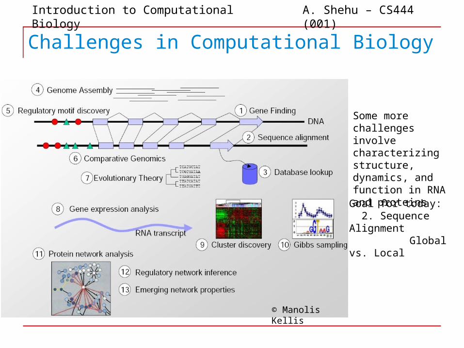
Challenges in Computational Biology
Some more challenges involve characterizing structure, dynamics, and function in RNA and proteins
Goal for today: 2. Sequence Alignment
Global vs. Local
© Manolis Kellis
Introduction to Computational Biology A. Shehu – CS444 (001)
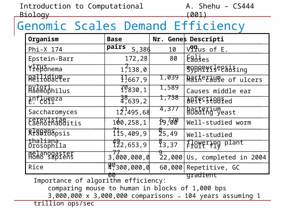
Genomic Scales Demand Efficiency
Haemophilus influenza
Heliobacter pylori
Treponema pallidium
Epstein-Barr virus
Phi-X 174
Organism
E. Coli
Saccharomyces cerevisiae
Caenorhabditis elegans
Arabidopsis thaliana
Drosophila melanogaster
Homo sapiens
Rice
Base pairs
5,386
172,282
1,138,011
1,667,970
1,830,138
4,639,221
12,495,682
100,258,171
115,409,949
122,653,977
3,000,000,000
4,300,000,000
10
Nr. Genes
60,000
22,000
13,379
25,498
19,000
5,770
4,377
1,738
1,589
1,039
80
Description
Virus of E. Coli
Causes mononucleosis
Syphilis-causing bacterium
Main cause of ulcers
Causes middle ear infections
Best-studied bacterium
Budding yeast
Well-studied worm
Well-studied flowering plant
Fruit fly
Us, completed in 2004
Repetitive, GC gradient
Importance of algorithm efficiency:comparing mouse to human in blocks of 1,000 bps3,000,000 x 3,000,000 comparisons → 104 years assuming 1 trillion ops/sec
Introduction to Computational Biology A. Shehu – CS444 (001)
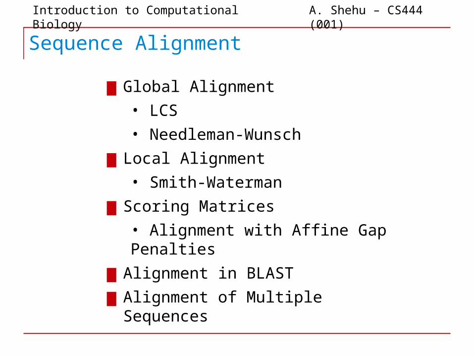
Sequence Alignment
▆ Global Alignment
• LCS
• Needleman-Wunsch
▆ Local Alignment
• Smith-Waterman
▆ Scoring Matrices
• Alignment with Affine Gap Penalties
▆ Alignment in BLAST
▆ Alignment of Multiple Sequences
Introduction to Computational Biology A. Shehu – CS444 (001)
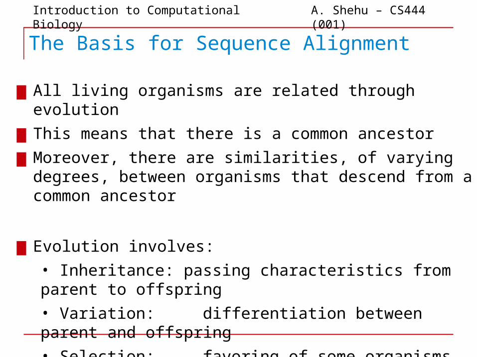
The Basis for Sequence Alignment
▆ All living organisms are related through evolution
▆ This means that there is a common ancestor
▆ Moreover, there are similarities, of varying degrees, between organisms that descend from a common ancestor
▆ Evolution involves:
• Inheritance: passing characteristics from parent to offspring
• Variation: differentiation between parent and offspring
• Selection: favoring of some organisms over others
Introduction to Computational Biology A. Shehu – CS444 (001)
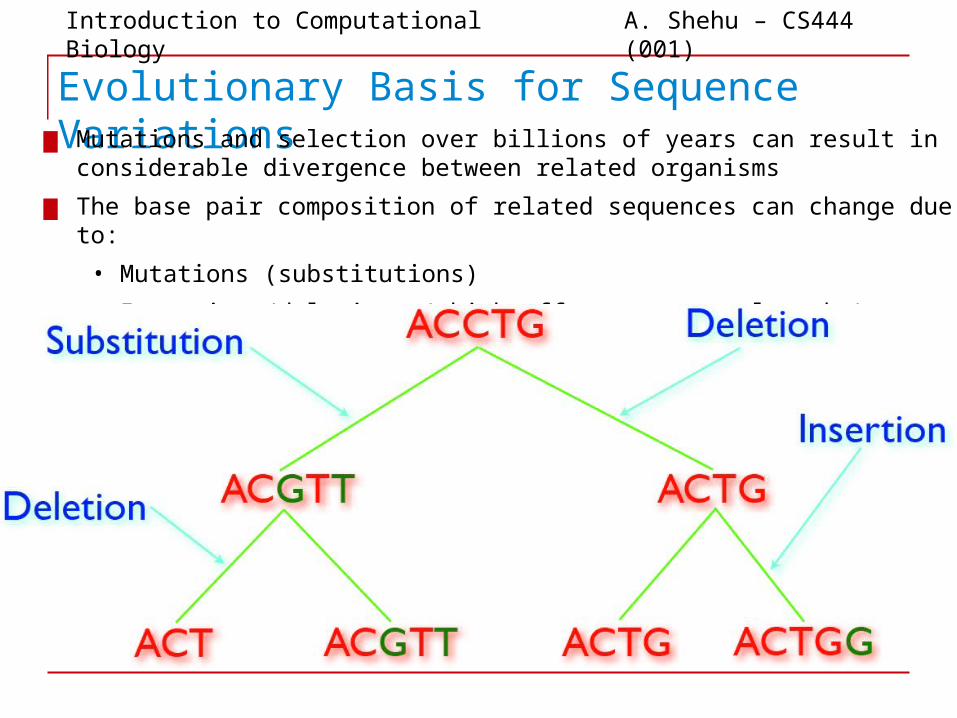
Evolutionary Basis for Sequence Variations▆ Mutations and selection over billions of years can result in considerable divergence
between related organisms
▆ The base pair composition of related sequences can change due to:
• Mutations (substitutions)
• Insertions/deletions (which affect sequence lengths)
Introduction to Computational Biology A. Shehu – CS444 (001)
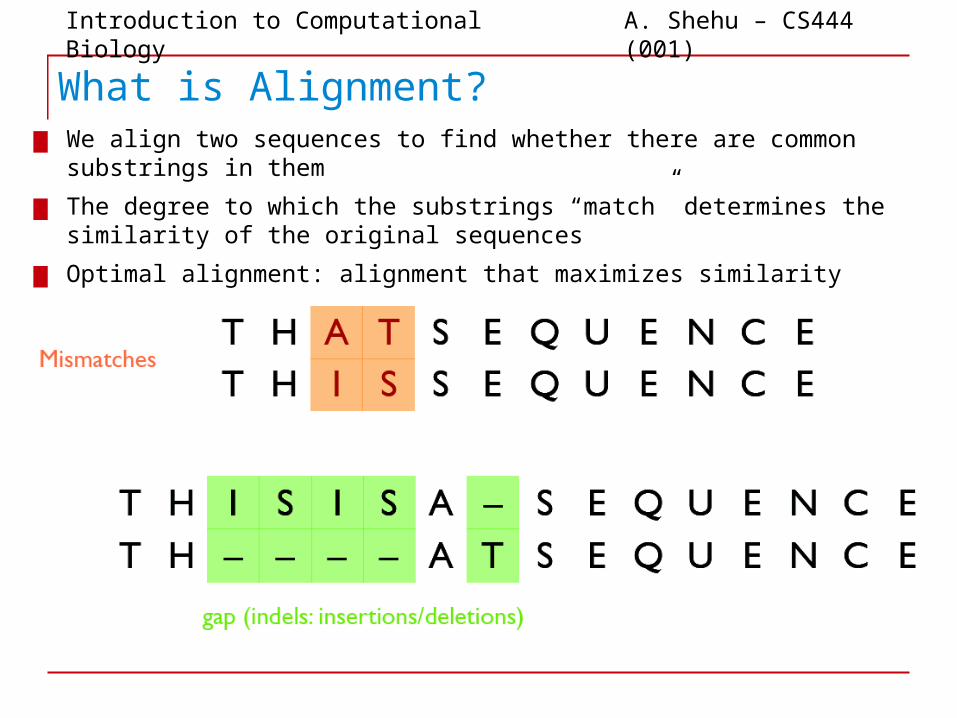
What is Alignment?▆ We align two sequences to find whether there are common substrings in them
▆ The degree to which the substrings “match” determines the similarity of the original sequences
▆ Optimal alignment: alignment that maximizes similarity
Introduction to Computational Biology A. Shehu – CS444 (001)
Sequence Similarity vs. Homology: Why do we Align?
▆ 1. Alignment can reveal whether two sequences are homologous or not
▆ Homologous sequences are those that descend from a common ancestor
• The sequences share a common ancestral sequence
▆ Note:
• Similarity is a descriptive term for degree of matching between two sequences
• Similarity does not automatically imply homology
• Sequences can be highly similar but not homologous (convergent evolution)
▆ 2. Alignment can be used to denote a common protein function
▆ Note:
• Sequence similarity does not always imply functional similarity
• Conserved function does not always imply sequence similarity

Introduction to Computational Biology A. Shehu – CS444 (001)
Why Align Protein over DNA Sequences?
▆ Easier to detect homology when comparing amino-acid sequences rather than nucleic acid sequences
• Why?
• Hint 1: There are only four bases in DNA/RNA (A, T/U, C, G)
• Hint 2: There are 20 (classic) amino acids in proteins
• The probability of a match by chance in DNA is ... than in a protein chain
• Another reason: genetic code is redundant
• What does this mean?
▆ A strong reason:
• Structure and function of a protein is determined by its amino-acid sequence
• Function conservation restricts changes that can happen to amino-acid sequence
▆ Our next goal:
• Global Alignment (Needleman-Wunsch) vs. Local Alignment (Smith-Waterman)
Introduction to Computational Biology A. Shehu – CS444 (001)
Global Alignment: Needleman-Wunsch
▆ The problem of global alignment when (1) matching characters exactly and (2) not penalizing for gaps (insertions or deletions) is a classic problem in computer science known as
• Longest Common Subsequence (LCS)
• Often presented to illustrate Dynamic Programming
• Short Detour: LCS lecture (Shehu_LCS.pdf)
▆ Reason to allow “soft” matching rather than exact matching:
• Amino acids with similar chemical properties and size can often replace one another with little effect to both structure and function
• Substitution matrices compiled over functionally-related proteins dictate penalty for soft matches or substitutions
▆ We also want to penalize gaps (indels):
• Needleman-Wunsch algorithm is the general version of LCS that takes into account both substitutions and gap penalties
Introduction to Computational Biology A. Shehu – CS444 (001)
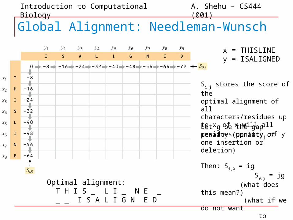
Global Alignment: Needleman-Wunsch
x = THISLINEy = ISALIGNED
Optimal alignment: T H I S _ L I _ N E _ _ _ I S A L I G N E D
Si,j stores the score of the
optimal alignment of allcharacters/residues up to x
i of
x will all residues up to yj of y
Let g be the gap penalty (penalty of one insertion or deletion)
Then: Si,0
= ig
S0,j
= jg
(what does this mean?) (what if we do not want
to penalize gaps at beginning or end?)

Introduction to Computational Biology A. Shehu – CS444 (001)
Only Difference from LCS in S matrix
▆ How is s(xi, yj) determined?
▆ What about the gap penalty?
▆ Answer: through a scoring matrix
• PAM, BLOSUM are examples of scoring matrices
• It is very important to have the “right” scoring matrix
Introduction to Computational Biology A. Shehu – CS444 (001)
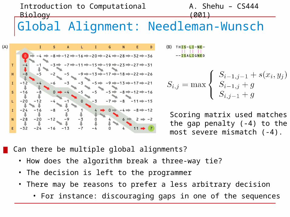
Global Alignment: Needleman-Wunsch
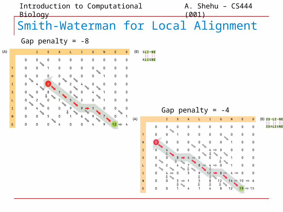
Scoring matrix used matches the gap penalty (-4) to the most severe mismatch (-4).
▆ Can there be multiple global alignments?
• How does the algorithm break a three-way tie?
• The decision is left to the programmer
• There may be reasons to prefer a less arbitrary decision
• For instance: discouraging gaps in one of the sequences
Introduction to Computational Biology A. Shehu – CS444 (001)
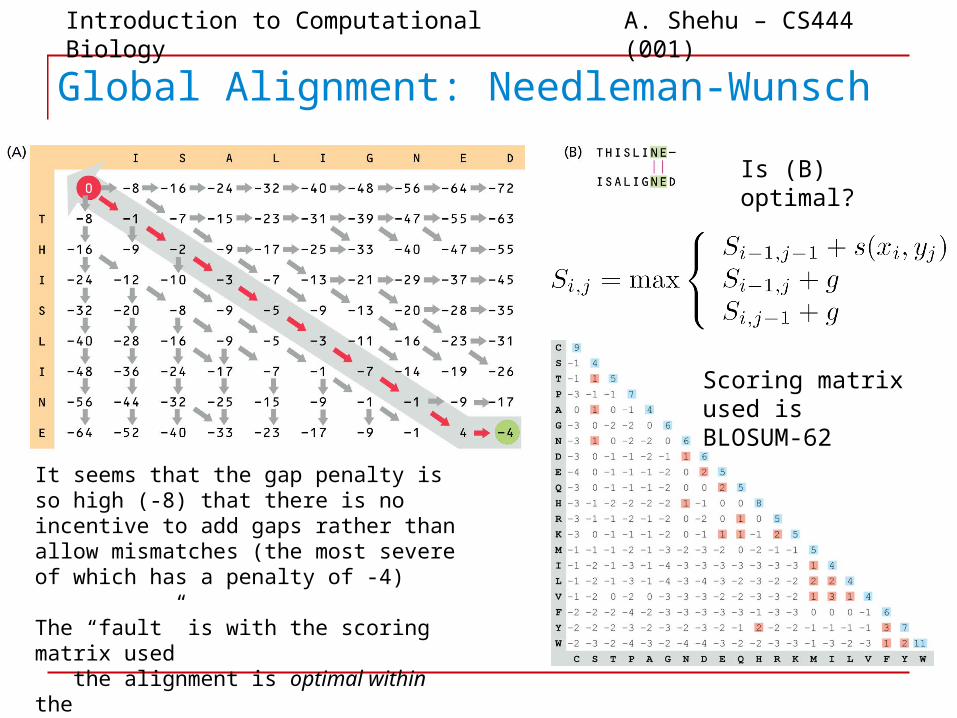
Global Alignment: Needleman-Wunsch
It seems that the gap penalty is so high (-8) that there is no incentive to add gaps rather than allow mismatches (the most severe of which has a penalty of -4)
The “fault” is with the scoring matrix used the alignment is optimal within the scoring matrix used
Is (B) optimal?
Scoring matrix used is BLOSUM-62
Introduction to Computational Biology A. Shehu – CS444 (001)
From Global to Local Alignment
▆ Sometimes local alignment is more appropriate than global alignment
• E.g., we want to determine whether two proteins share a common domain
• The Smith-Waterman algorithm addresses local alignment
What does the rejection of a negative optimal sub-alignment mean? Hint: many mini global alignments not worth to continue at some point
▆ Main differences over Needleman-Wunsch:
• Whenever the score of the optimal sub-alignment is less than zero, it is rejected (the matrix element is set to 0)
• Traceback starts from the highest-scoring element
0
Introduction to Computational Biology A. Shehu – CS444 (001)
Smith-Waterman for Local AlignmentGap penalty = -8
Gap penalty = -4
Introduction to Computational Biology A. Shehu – CS444 (001)
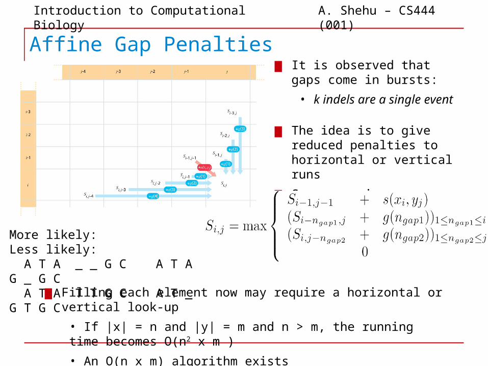
Affine Gap Penalties▆ It is observed that gaps come
in bursts:
• k indels are a single event
More likely: Less likely: A T A _ _ G C A T A G _ G C A T A T T G C A T _ G T G C
▆ The idea is to give reduced penalties to horizontal or vertical runs
▆ Score now is:
▆ Filling each element now may require a horizontal or vertical look-up
• If |x| = n and |y| = m and n > m, the running time becomes O(n2 x m )
• An O(n x m) algorithm exists
Introduction to Computational Biology A. Shehu – CS444 (001)
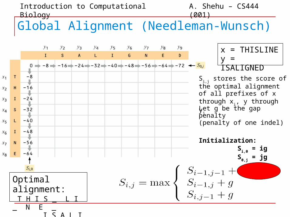
Global Alignment (Needleman-Wunsch)
x = THISLINEy = ISALIGNED
Optimal alignment: T H I S _ L I _ N E _ _ _ I S A L I G N E D
Si,j stores the score of the optimal
alignment of all prefixes of x through x
i, y through y
j
Let g be the gap penalty (penalty of one indel)
Initialization: S
i,0 = ig
S0,j
= jg
Introduction to Computational Biology A. Shehu – CS444 (001)
Scoring Scheme
▆ Consists of two elements:
1. Substitution matrix Assigning a value to a pair of aligned residues
2. Gap model Dealing with the presence of indels in one sequence relative to the other
Introduction to Computational Biology A. Shehu – CS444 (001)
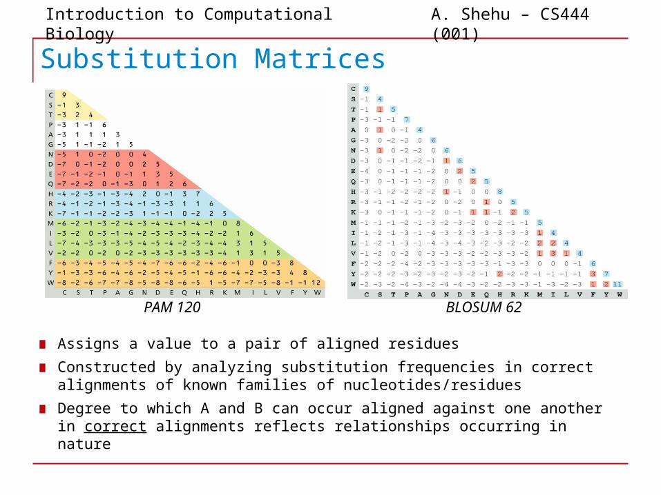
Substitution Matrices
▆ Assigns a value to a pair of aligned residues▆ Constructed by analyzing substitution frequencies in correct
alignments of known families of nucleotides/residues▆ Degree to which A and B can occur aligned against one another
in correct alignments reflects relationships occurring in nature
PAM 120 BLOSUM 62
Introduction to Computational Biology A. Shehu – CS444 (001)
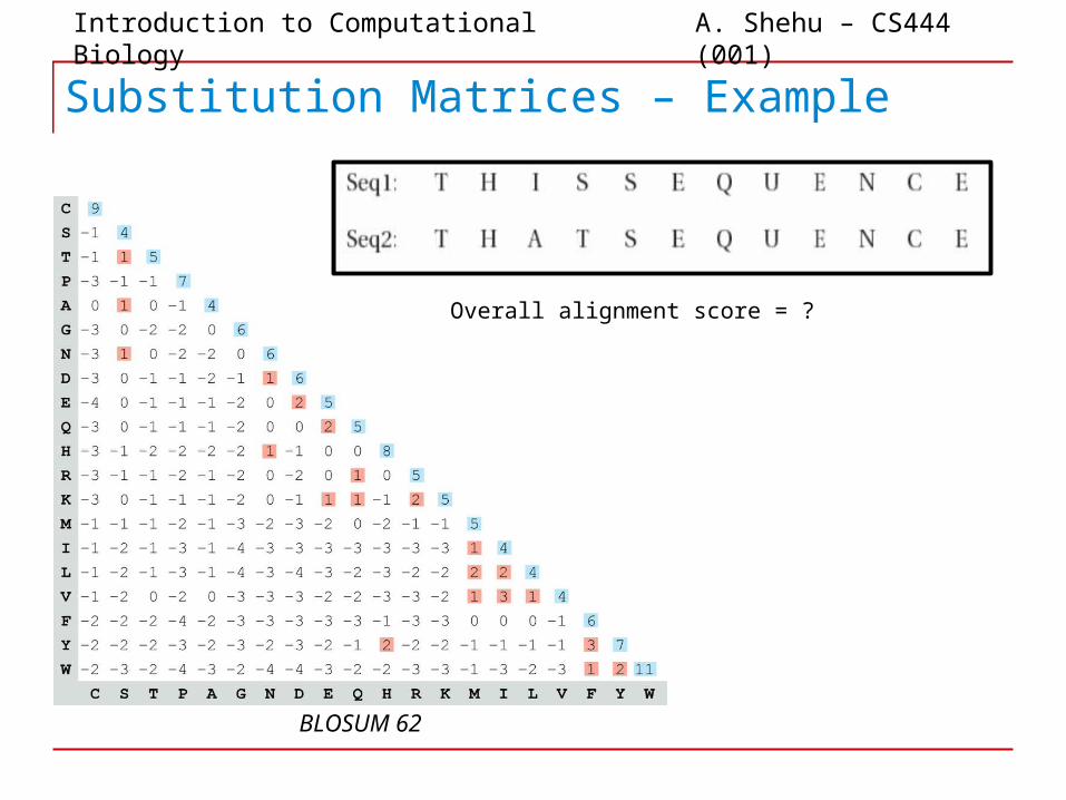
Substitution Matrices – Example
BLOSUM 62
Overall alignment score = ?

Introduction to Computational Biology A. Shehu – CS444 (001)
Substitution Matrices – Example
Overall alignment score: 52
BLOSUM 62
Introduction to Computational Biology A. Shehu – CS444 (001)
Scoring Matrices: How are they Constructed?▆ Scoring matrices are created based on biological evidence
▆ Statistics over protein sequences are gathered
▆ Some mutations have little effect on the protein’s function
▆ Reason why some penalties δ(vi , wj), are less harsh than others
▆ The statistics is a bit more involved
▆ The alignment score attempts to measure the likelihood of a common evolutionary ancestor
▆ To achieve this mathematically, the alignment of two residues from two sequences is considered under two competing models/hypotheses:
▆ The random model (R)
▆ The match (non-random, evolutionary) model, M

Introduction to Computational Biology A. Shehu – CS444 (001)
The Random vs. the Match Model
▆ Sequences are assumed to be random selections from a given pool of residues
▆ Every position in the sequence is independent of every other
▆ If the proportion of amino acid type a in the pool is pa, this fraction will be
reproduced in a sequence
▆ As a result, the probability of amino acid a being aligned with amino acid b is pa x pb
The Random Model:
▆ Sequences are assumed to be related due to an evolutionary process, with a high correlation between aligned residues
▆ The probability of occurrence of particular residues depends not on the pool of available residues, but on the residue at the equivalent position in the sequence of the common ancestor
▆ As a result, the probability of a being aligned with b is qa,b, where the actual values of qa,b depend on the properties of the evolutionary process
The Match Model:
Introduction to Computational Biology A. Shehu – CS444 (001)
The Random vs. the Match Model: the Odds Ratio
▆ P(a,b|R) = pa x pb and P(a,b|M) = qa,b
▆ Comparing the odds: qa,b/papb
▆ If the ratio is greater than 1, we say that the match model is more likely to explain the alignment of a to b
▆ The odds ratio over two aligned sequences is the product of the above ratio for the different positions
▆ The product turns into a summation under the logarithm
▆ That is why scores are summed up when computing the alignment either in Needleman-Wunsch or Smith-Waterman
▆ A positive score means that the match model explains the alignment at that position
▆ What does a negative score mean?
▆ Two scoring matrices: PAM and BLOSUM

Introduction to Computational Biology A. Shehu – CS444 (001)
PAM (Point Accepted Mutation) Scoring Matrix
▆ Scoring matrices are best developed based on experimental data because in this way they reflect the actual relationships that occur in nature
▆ PAM was one of the first scoring matrices – developed by Dayhoff et al.
▆ Substitution probabilities were estimated by using known mutational histories
▆ 34 protein superfamilies were used, divided into 71 groups of near--homologous sequences (>85% identity to remove superimposed mutations)
▆ A phylogenetic tree was constructed for each group (including inference of most likely ancestral sequences at each internal node)
▆ We have not yet covered phylogeny, but it is used to define an evolutionary model that explains the evolution
▆ Caviat: even under the evolutionary model, the substitution in a position is independent of what happens in neighboring positions
▆ This is not always a valid assumption
Introduction to Computational Biology A. Shehu – CS444 (001)
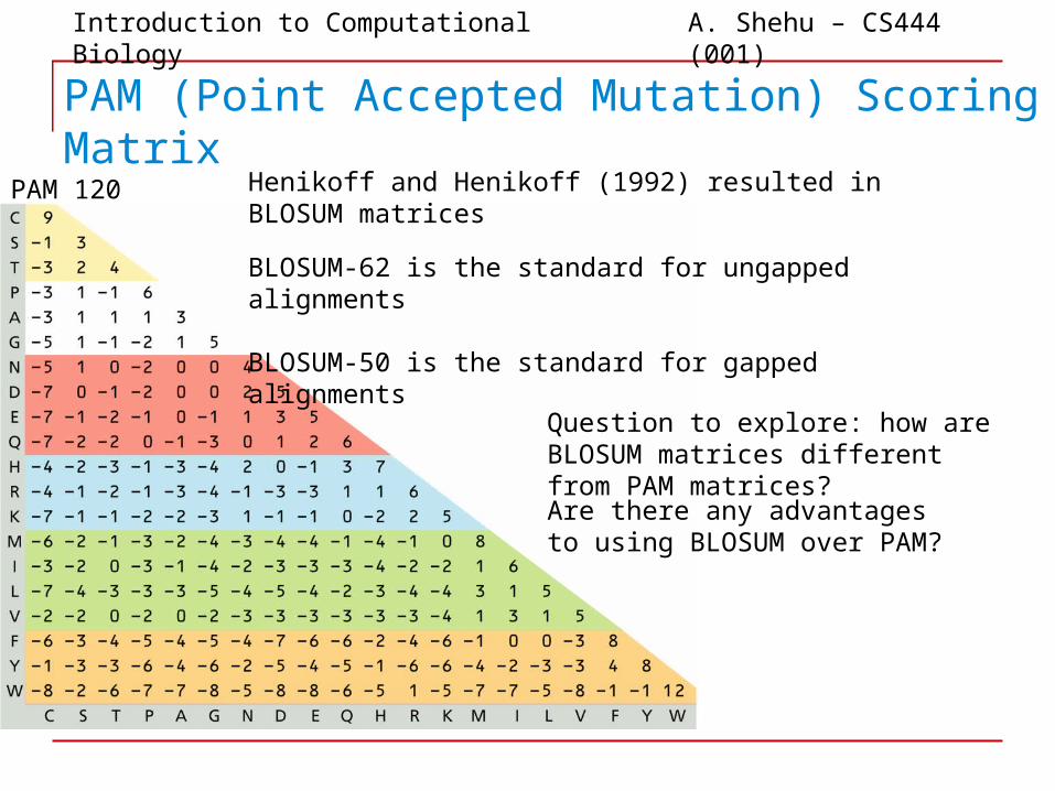
PAM (Point Accepted Mutation) Scoring Matrix
PAM 120
Question to explore: how are BLOSUM matrices different from PAM matrices?
Are there any advantages to using BLOSUM over PAM?
BLOSUM-62 is the standard for ungapped alignments
BLOSUM-50 is the standard for gapped alignments
Henikoff and Henikoff (1992) resulted in BLOSUM matrices
Introduction to Computational Biology A. Shehu – CS444 (001)
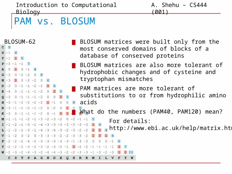
PAM vs. BLOSUM
▆ BLOSUM matrices were built only from the most conserved domains of blocks of a database of conserved proteins
▆ BLOSUM matrices are also more tolerant of hydrophobic changes and of cysteine and tryptophan mismatches
▆ PAM matrices are more tolerant of substitutions to or from hydrophilic amino acids
▆ What do the numbers (PAM40, PAM120) mean?
BLOSUM-62
For details:http://www.ebi.ac.uk/help/matrix.html
Introduction to Computational Biology A. Shehu – CS444 (001)
Which Scoring Matrix to Use?
▆ PAM* vs. BLOSUM*: This decision is also more difficult when the evolutionary distance between the sequences is not known
▆ Different studies have concluded that for the PAM matrices it is generally best to try PAM40, PAM120, and PAM250
▆ BLOSUM matrices are best for local alignments
▆ If using PAM for local alignments:
▆ Lower PAM matrices find short local alignments
▆ Higher PAM matrices find longer but weaker local alignments
▆ Several different matrices should be used, and the alignment that is judged to be evolutionarily the most accurate is the one chosen
▆ Question: how can one judge which one is the most accurate?
▆ Judgment on a control set where the evolutionary relationship is known
Introduction to Computational Biology A. Shehu – CS444 (001)
Gaps
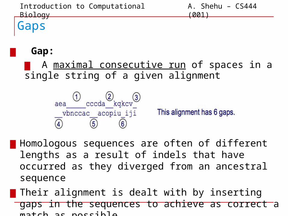
▆ Gap:
▆ A maximal consecutive run of spaces in a single string of a given alignment
▆ Homologous sequences are often of different lengths as a result of indels that have occurred as they diverged from an ancestral sequence
▆ Their alignment is dealt with by inserting gaps in the sequences to achieve as correct a match as possible
Introduction to Computational Biology A. Shehu – CS444 (001)
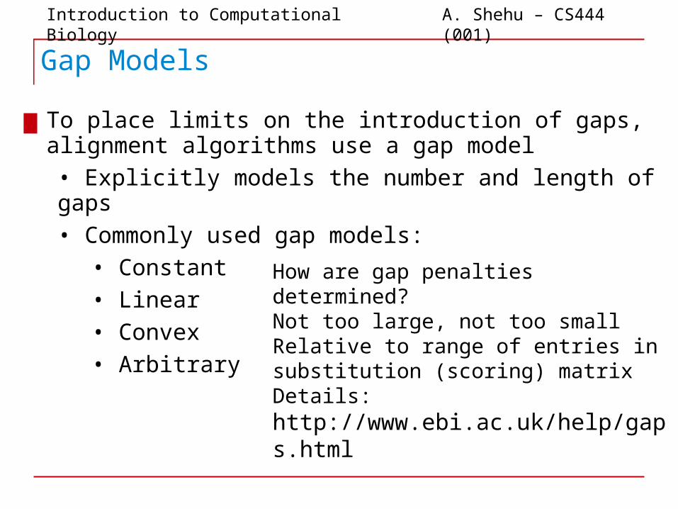
Gap Models
▆ To place limits on the introduction of gaps, alignment algorithms use a gap model
• Explicitly models the number and length of gaps
• Commonly used gap models:
• Constant
• Linear
• Convex
• Arbitrary
How are gap penalties determined?Not too large, not too smallRelative to range of entries in substitution (scoring) matrix
Details: http://www.ebi.ac.uk/help/gaps.html
Introduction to Computational Biology A. Shehu – CS444 (001)
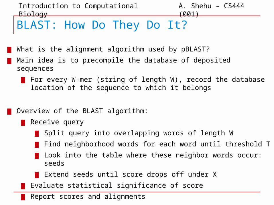
BLAST: How Do They Do It?
▆ What is the alignment algorithm used by pBLAST?
▆ Main idea is to precompile the database of deposited sequences
▆ For every W-mer (string of length W), record the database location of the sequence to which it belongs
▆ Overview of the BLAST algorithm:
▆ Receive query
▆ Split query into overlapping words of length W
▆ Find neighborhood words for each word until threshold T
▆ Look into the table where these neighbor words occur: seeds
▆ Extend seeds until score drops off under X
▆ Evaluate statistical significance of score
▆ Report scores and alignments

Introduction to Computational Biology A. Shehu – CS444 (001)
BLAST: Illustration
Seeds are extended until the cumulative score drops
Karlin-Altschul statistics P-value: Probability that the HSP was generated by chance Score: -log(probability) E: expected number of such alignments given the database
Question: What is a two-hit blast?


