48
A Short Introduction to GIS C. D. Lloyd School of Environmental Sciences University of Liverpool Copyright © C. D. Lloyd, 2012

A Short Introduction to GIS
C. D. Lloyd
School of Environmental Sciences University of Liverpool
Copyright © C. D. Lloyd, 2012

ii
Contents
Preface ........................................................................................................... iii Acknowledgements ......................................................................................... iii Basic principles and data models
Chapter 1. Introduction to GIS ......................................................................... 1
Chapter 2. Spatial data models and data input ................................................ 4
Chapter 3. Databases in GIS ........................................................................... 8
Spatial data analysis
Chapter 4. Analysis of objects ....................................................................... 10
Chapter 5. Analysis of grids and surfaces ...................................................... 19
Data visualisation and data quality
Chapter 6. Visualisation and presentation of spatial ...................................... 27
information ..................................................................................................... 27
Chapter 7. Data quality .................................................................................. 31
Organisation and application of GIS
Chapter 8. GIS project design, management and organization ..................... 34
Chapter 9. Applications of GIS ....................................................................... 36
Future developments and summary
Chapter 10. GIS in the future ......................................................................... 42
References .................................................................................................... 44

iii
Preface
This booklet is intended as a very brief introduction to the principles and practice of
Geographical Information Systems and Science. The coverage of some material is
intentionally limited, but there is hopefully enough depth to help develop
understanding and guide further reading. At the end of each chapter some
recommended references are given.
This booklet is intended primarily for students attending the module
ENVS363/ENVS563 ‘Geographical Information Systems’ at the University of
Liverpool. It may be used for teaching purposes by anyone else on the condition that
is it properly cited. Citation should follow this format:
Lloyd, C. D. (2012) A Short Introduction to GIS. Liverpool: School of Environmental
Sciences, University of Liverpool.
Please contact the author with any comments or suggestions (email address:
Acknowledgements
Conor Graham is thanked for allowing the use of case study material in Chapter 9.

1
Chapter 1. Introduction to GIS
This chapter introduces the topics of spatial data and Geographical Information
Systems (GIS). One possible definition of a GIS is that it is a software environment
for collecting, storing, managing, analyzing and visualizing spatial data (as defined in
Section 1.1). Other definitions are considered in Section 1.4. Section 1.4 also
introduces the notion of Geographical Information Science.
The chapter will provide you with a summary of the basic concepts and the themes
outlined will be discussed in more detail in later chapters.
1.1 What are spatial data?
One of the reasons that GIS are different to other information systems is that they are
used to work with spatial data. Spatial data are data that have some attribute that can
be used to position them in space. This spatial information may comprise, for
example, grid co-ordinates or postcodes. Examples of aspatial (that is, non spatial)
and spatial data are shown in Figure 1.1.
Figure 1.1. Aspatial data and spatial data.
1.2 Sources of spatial data
Spatial data may be collected by, or on behalf of, the user (primary data) or data
collected by others may be input into a GIS (secondary data).
There are two ways in which (primary) spatial data may be collected:
• Ground survey: contact is generally made with the property of interest during its
measurement
• Remote sensing: no physical contact is made with the property of interest during its
measurement
Alternatively, existing data may be suitable. Information in paper maps may be input
into a computer using several procedures including digitisation and scanning.

2
The topic of sources of spatial data will be addressed in more detail in Chapter 2.
1.3 Analysing spatial data
Once we have some spatial data we can analyse them (note data = plural, datum =
singular) in one of two ways. We can:
• Summarise or describe the data as though they are not spatially referenced
• Take into account the spatial location of one variable or assess spatial relationships
between variables
There may be a wide range of problems that we have to resolve using spatial data. Put
simply, we may wish to ascertain:
• Where are particular features found?
• What geographical features exist?
• What changes have occurred over a given time?
• Where do certain conditions apply?
• What will the spatial implications be if an organisation takes certain action?
(Source: Heywood et al., 2006)
The following questions detail some specific examples of problems that involve
spatial data:
• How many houses are located within two kilometres of a planned power station?
• What is the shortest route between an ambulance station and the site of an accident?
• What areas lie more than one kilometre from reservoirs, are undeveloped,
unpolluted, and on gravely soils?
• What are the characteristics of some property (e.g., amount of rainfall) at some
unsampled location?
Each of these problems concerns the spatial relations between several variables (for
example, distances between some houses and a power station). These kinds of
problems can be solved using the tools provided within a Geographical Information
System (GIS).
Applications in which GIS have been used are extensive. GIS are widely used in
maintaining, analysing and displaying many different kinds of data that are spatially
referenced, such as locations of pollution monitoring stations, topographic features or
outbreaks of disease.
It is usually the case that the data in a GIS are stored in a series of ‘layers’. Taking the
first problem stated above: the data would comprise a layer with information about
the location of houses and a layer giving the site of the proposed power station. The
analytical functionality (in other words, the analysis tools) of the GIS would then be
used to calculate the distance between the planned power station and each of the
houses in the data set. Each of the houses within the specified distance of the power
station could then be selected and highlighted using the GIS.

3
1.4 Geographical Information Systems and Science
GIS have been developed to enable us to map and, more specifically, to analyse
spatial information. There are many definitions of GIS but one which summarises the
key components well views GIS as “a powerful set of tools for collecting, storing,
retrieving at will, transforming and displaying spatial data from the real world for a
particular set of purposes” (Burrough, 1986).
GIS does not stand still and the field of study that deals with developments that are
made in response to problems faced when using a GIS is called Geographical
Information Science (GIScience; see Longley et al., 2005a, for more details). The
acronym GIS is used in this resource to refer to GISystems and where GIScience is
meant this is made clear.
This guide introduces the basic principles of GIS and GIScience. The resource is
divided into four parts, defined as follows:
Basic principles and data models (this chapter and Chapters 2 and 3): discusses
how spatial features are represented in a GIS as well as data collection and input.
Spatial data analysis (Chapters 4 and 5): focuses on the key set of functions that
make a GIS different to other information systems, the ability to analyse spatial
variation.
Data visualisation and data quality (Chapters 6 and 7): reviews the main
approaches to visualising spatial data in a GIS.
Organisation and application of GIS (Chapters 8 and 9): a key component of an
GIS is the way in which it is set up and operated, this part of the guide reviews the
organisation of GIS and looks at some case studies.
The final chapter (9) is concerned with recent and possible future developments in
GIS.
1.5 Further reading
Each chapter has at its ends a list of recommended texts that should be used to
develop your theoretical knowledge of GIS. Good general introductions to spatial data
and GIS are the books by Burrough and McDonnell (1998), Heywood et al. (2006)
and Longley et al. (2005a).
The next chapter deals with the representation of spatial features in a GIS, sources of
spatial data and the input into GIS of information from existing paper-based sources.

4
Chapter 2. Spatial data models and data input
This chapter deals with two issues: (i) how reality is represented in a GIS and (ii)
sources of spatial data. The chapter will describe the two main data models used in
GIS and the key means of acquiring spatial data will be outlined.
2.1 Spatial data models
Spatial information may be represented in a computer in variety of ways. In other
words, reality may be modelled, abstracted, or represented using different approaches.
The two main data models in GIS are called vectors and rasters.
Vector data comprise points, line and polygons (enclosed areas). The vector model is
illustrated in Figure 2.1. Rasters are images or grids comprising cells called pixels.
The raster model is illustrated in Figure 2.2. The vector and raster models are
described in more detail below.
Figure 2.1. The vector model. Figure 2.2. The raster model.
In Figure 2.1, the point feature could be the location of a well hole; the line could
represent a road and the polygon (an area) would be a suitable means of representing
a lake. Vector lines and polygons are composed of nodes (the dots in Figure 2.1 with
co-ordinates next to them), arcs, the lines that connect nodes to one another and
vertices. Vertices represent changes in direction of arcs. Vector data comprise (i)
spatial information (that is, their location defined by co-ordinates and topological
information for lines and polygons) and (ii) attribute information (such as a line which
carries the attribute ‘road’).
In Figure 2.2, the cells are shaded according to the numbers assigned to them. Cells
(or pixels) with the value 1 (coloured white) could represent, for example, a low level
of pollution whilst cells with a value of 4 (coloured black) could represent a high level
of pollution. Unlike vector data, the cells in a raster grid do not have information
stored concerning their location. Rather, the location of a cell is known within a grid
(that is, a cell may be in fourth position along the x axis and seventh position along
the y axis). In other words, a cell is not considered a separate object. The area covered
on the ground by a cell is referred to as its spatial resolution. So, a grid with a spatial
resolution of 5 metres has cells that cover an area of 5 by 5 metres in the real world.

5
The vector model is commonly used to represent discrete feature such as ‘road’,
‘park’ or ‘county boundary’. In contrast, raster grids are primarily used to represent
continuous variables such as ‘elevation’, ‘precipitation’ or ‘soil acidity’. Exceptions
are when vectors are used to represent topography (for example, using contour lines)
and digital remotely sensed imagery (raster grids) which may include a range of
different objects such as houses, trees or water.
One of the most important decisions that must be made when a spatial database is
established concerns whether to use the vector or raster data model. The choice
between the two is not always straightforward and it will depend on many factors, not
least of which is the availability of digital data. Where the data are input by the user
then clearly there is greater choice.
Once spatial data are available in a digital format it is usually fairly straightforward to
convert between data formats, for example vector to raster conversion. In addition,
there is often a desire to convert data to different co-ordinate systems, this is a
standard function of most GIS.
2.2 Spatial data collection and input
Data may be divided into two classes: primary data and secondary data. Primary data
are acquired by the user for a specific purpose. Secondary data are data collected by
another group or individual. A common limitation of GIS analyses is that the data
used may have been collected with a purpose in mind which is different to that for
which the data are required. Thus, they may not be ideally suited to task in hand.
2.3 Primary data
Spatial data may be collected on the ground or through remote sensing. There are
several widely used means of obtaining information on the spatial position of features
through ground survey. These include:
• Traditional survey techniques: tape and offset surveying and levelling.
• Theodolites (for measuring angles).
• Electronic Distance Measurers (EDMs).
• Total stations: high precision theodolite and an EDM.
• Global Positioning Systems (GPS).
As well as conventional aerial photography remotely sensed data may be obtained
through the use of different kinds airborne and spaceborne sensors which detect
radiation from different parts of the electromagnetic spectrum. Sensors may be
divided into two groups:
• Passive sensors: sense naturally available energy.
• Active sensors: supply their own source of energy to illuminate selected features.
Examples are radar and LiDAR (Light Detection and Ranging). Radar emits pulses of
macrowave energy and LiDAR emits pulses of laser light.

6
2.4 Secondary data
Data may be converted from an analogue format (for example, a paper map) into a
digital format using several different approaches. These include keyboard entry,
digitisation and scanning. Each of these approaches are summarised below.
Keyboard entry: Spatial attributes (for example, co-ordinates or postcodes) and non-
spatial information (for example, descriptions of the features being mapped) are input
manually.
Digitisation: features are traced using either a mouse (for on-screen digitising) or a
puck (for digitising features on a paper map).
Scanning: the source document (for example, a map) is sampled using transmitted or
reflected light.
The basic principles of digitising can be summarised as follows:
• The digitiser works on the basis that it is possible to ascertain the location of a puck
(rather like a mouse) as it passed over a table that is inlaid with a fine mesh of wires.
• Digitising results in vector representation of the features traced.
• Digitising can also be conducted on-screen by using the mouse cursor to trace
features (for example, you could trace roads on a scanned aerial photograph). On-
screen digitising is also called heads-up digitising.
• Digitisers can be set only to record points each time the puck button is pressed
(point mode). Alternatively, stream mode can be used. In stream mode, the digitiser
can be set to record points when the cursor moves for a set distance or period of time.
Figure 2.3 shows a digitiser in use. The operator is tracing the features on a map using
a puck which has a clear window with a cross-hair superimposed with which the map
features are traced.
Figure 2.3. Digitising in action.
The key steps in the digitising process are as follows:
1. The paper map is taped to the digitising tablet.
2. Control points are selected on the map.
3. The control points are entered one at a time to register the map to the tablet.
4. Features are traced using the cursor.
5. After completion of step 4 the digitised features are checked for errors.

7
6. Attribute data are added.
The basic principles of scanning can be summarised as follows:
• The scanner works by scanning line by line across an analogue source (e.g., a paper
map) and recording the amount of light reflected from the surface of the data source.
• The map is scanned in using a drum scanner (a flat bed scanner may also be used if
accuracy is less of a concern).
• Scanning results in a new raster (cell-based) representation of the map. Features on
the map must be identified as objects as a separate step.
2.5 Further reading
There are many good introductions to the principles of spatial data models and data
input. The books by Burrough and McDonnell (1998), Heywood et al. (2006) and
Longley et al. (2005a) all provide information on these issues. In addition, Part 2,
Section C of the book edited by Longley et al (2005b) provides detailed accounts of
specific issues in spatial data collection.
The next chapter looks at databases in GIS, the database is the core of a GIS and a
well designed database is central in allowing efficient and rapid access to the data
stored within the system.

8
Chapter 3. Databases in GIS
GIS was defined in Chapter 1. One definition of GIS is that it is a spatial database.
That is, GIS store data like any other database. The difference with other databases is
that in a GIS the data are spatially referenced — they have a spatial location.
As was noted in Chapter 2, vector data are composed of spatial information and
attribute information. Spatial data may be input into the GIS by manual input,
scanning or digitising (as detailed in Chapter 2) but in these cases attribute data are
keyed in separately. Each of the spatial features, such as a length of road, is assigned
unique identifiers. If the attribute data stored in a spreadsheet or database have the
same identifiers then the spatial and attribute information can be linked. This, of
course, enables the user to select and draw features with specific attributes. Before
looking at this concept in a little more detail the chapter will define databases.
3.1 Defining a database
A database is a set of structured data — “An organised filing cabinet is a database, as
is a dictionary, telephone directory, or address book. Thus, databases can be
computer-based or manual” (Heywood et al., 2006, p. 111). Once information is
stored in a computer-based database it can be sorted, summarised and combined in
various ways. For a database to be useful it must contain appropriate data that can be
accessed effectively and efficiently.
3.2 Database Management Systems
Data stored in databases are managed and accessed using a database management
system (DBMS). If, for example, you wished to extract all records in a database that
fulfilled certain conditions (for example all shops with more than 25 staff) then you
would use DMBS computer software to achieve this. Structured Query Language
(SQL) is a language that has been developed to enable users to access information in a
database in a fairly flexible way.
3.3 The relational database
Various different approaches to storing data in computers have been developed. The
most widely used form of database at the present time is called a relational database.
The relational data model was introduced by Codd (1970). In a relational database,
data are organised in a set of two-dimensional tables. Each table contains information
for one entity (for example, the table ‘Cinemas’, may contain information about the
addresses of different cinemas and the number of screens they have). Different tables
are linked by identifiers called keys.
Figure 3.1 illustrates how, in a relational database, spatial features are linked to
attribute data tables that may be linked to further attribute data tables.

9
Figure 3.1. Storage of spatial and attribute information in a relational database.
In Figure 3.1, the field ID is the common key that links the two tables. The table
containing co-ordinate information is linked to the arcs (line features) by unique
numbers (that is, there is only one arc and table entry with the value 1).
3.4 Further reading
The books by Burrough and McDonnell (1998), Worboys and Duckman (2004),
Heywood et al. (2006) and Longley et al. (2005a) all provide discussions about
databases and DBMS. More in-depth accounts on specific issues are provided in Part
2, Section B of the book edited by Longley et al (2005b).
The next chapter deals with the analysis of objects in a GIS.

10
Chapter 4. Analysis of objects
4.1 Introduction
At the heart of GIS is the capacity to analyse data – to explore patterns or answer
specific questions and to derive information from these data. It is easy to think of
many problems that entail analysing the spatial distribution of objects or events. Some
questions we may be interested in asking include:
1. Is there a link between cases of childhood leukaemia and the location of a power
station?
2. Does a particular mineral cluster in a rock?
3. How many houses are located with 10 km of a road?
4. What areas comprise high quality soil and low levels of industrial contamination?
5. Does the relationship between altitude and precipitation vary across Ireland?
6. What is the value of precipitation at a location where no measurements have been
made?
7. Which areas have a slope of greater than 25 degrees?
8. What is the shortest road route between one place and another given the need to
visit three particular locations on route?
This chapter and the next introduce a range of methods that can be used to help
answer some of the kinds of questions given above. GIS analysis tools may be divided
into several groups as follows (with the chapter that outlines the methods given in
parenthesis):
1. Point pattern analysis (quadrat analysis etc) (this chapter).
2. Grids and modelling (Chapter 5).
3. Single layer operations (univariate statistics, buffers) (this chapter).
4. Multiple layer operations (proximity analysis, overlay etc) (this chapter).
5. Surface analysis (Chapters 5).
6. Network analysis (network connectivity, shortest path etc.) (this chapter).
7. Spatial modelling (identification “of explanatory variables that are significant to
the distribution of the phenomenon…” (Chou, 1997, 265)).
(Modified from Chou, 1997)
Spatial modelling (no. 7 above) is outside the remit of this resource. A variety of text
books (e.g., Burrough and McDonnell, 1998) provide discussions about spatial
modelling.
This chapter deals with objects (often, although exclusively, represented using
vectors) while the following chapter is concerned with continuous variables (e.g.,
elevation or precipitation amount, often represented using raster grids).
The following section is concerned with the simplest form of object – the point
location.

11
4.2 Point pattern analysis
A point pattern is simply a set of events or points within a specific study area. There is
often a desire to assess how clustered or dispersed such data are. Alternatively, we
may be concerned with assessing how similar two point patterns are. Clustered and
dispersed point patterns are shown in Figure 4.1.
Figure 4.1. Left: clustered point pattern. Right: dispersed point pattern.
Examination of point patterns in the form of scatter plots (that is, a simple plot of the
location of the points) provides a sensible first step in the analysis of a point pattern.
This enables a first impression of the tendency towards clustering or regularity and
also local variation in the point pattern. However, to gain an idea of how clustered a
point pattern is it is necessary to estimate statistics that summarise in various ways
properties of the point pattern.
Simple summaries of spatial point patterns include the mean centre and the standard
distance. The mean centre is the mean x and mean y co-ordinates and the standard
distance measures the dispersion around the mean (that is, it tells us something about
the range of point locations) (see Lloyd, 2010, for more detail).
Quadrat analysis is one widely used method for analysing point patterns. In quadrat
analysis, a set of areas are superimposed on the region containing the points we are
analysing. Quadrat analysis entails using either (i) a set of quadrats covering the
whole of the area of interest or (ii) placing quadrats randomly across the area of
interest (this latter approach is often used in fieldwork). In either case, we count the
number of points within each quadrat and we can map the counts to get a sense of
whether or not there are clusters — areas where the density of points is high. There
may be a need to know if spatial variation in a particular property is structured — that
is, do values of a particular property tend to more similar when the observations are
close together than when they are far apart? Spatial structure is expressed by the term
spatial autocorrelation. One approach is to carry out a quadrat analysis and then
estimate the degree of spatial autocorrelation by comparing the counts of points in
adjacent quadrats. If, for example, the results of an analysis of spatial autocorrelation
indicate that quadrats containing large numbers of points occur close to other quadrats
with large numbers of points while quadrats with small numbers of points tend to

12
occur next to other quadrats with small numbers of points then the results indicate
clustering.
There are many other methods for analysing spatial point patterns. Kernel estimation
(KE) is a method for generating maps that show the estimated intensity of points
across the area of interest. That is, KE enables estimation of the intensity of points at
all locations in the area of interest irrespective of whether or not there is a point at any
particular location. Another class of methods use the distances between points to
analyse point patterns. For example, the mean nearest neighbour distance is the
average of the distances between each point and its nearest neighbour. For clustered
point patterns, the mean nearest neighbour distance will be smaller than for dispersed
point patterns.
A widely used method for analysing distances between points is the K function (see
Lloyd, 2010, for a detailed introduction). The K function summarises the number of
points separated from each point by specific distances. The K function can be
obtained by (i) finding all points within radius r of an event (that is, a point) and (ii)
counting these and calculating the mean count for all events after which the mean
count is divided by the overall study area event density which gives the K function for
a particular distance, (iii) the radius is then increased by some fixed step and (iv)
repeating steps (i), (ii) and (iii) to the maximum desired distance. The output from the
last stage for each distance can be plotted against the distance. The K function
provides information on how clustered a point pattern is at different scales. Knowing
about how many of a point’s neighbours are close, and how many are far away, tells
us something about the spatial structure of the point pattern we are analysing.
The measures discussed in previous sections provide various ways of assessing the
degree of clustering or dispersion of a point pattern. To consider how clustered or
how dispersed a point pattern is there is a need to use a statistical test of some kind.
This is often achieved my considering if an observed process is likely to be an
outcome of some hypothesized process (for example, in effect, are the locations of the
points due to some random process or are the points a function of some process that
causes them to cluster?). Models of complete spatial randomness (CSR) are used
widely. For a CSR process the intensity is constant (that is, each location has an equal
chance of containing an event) and events are independently distributed. There are
various tests that can be applied to assess if a point pattern corresponds to a CSR
process. In other words, such tests enable us to assess if the point pattern appears to be
random or if there is some structure in it.
Most GIS have some functions that enable the user to analyse point patterns, but these
are often limited.
4.3 Single layer operations
This chapter introduces some methods for analysis using single variables or objects.
Univariate statistics (e.g., the mean average or standard deviation) may be estimated
from single properties in a GIS, but the focus here is on spatial methods.

13
4.3.1 Computing distances
One of the most commonly-applied tasks in GIS is computing distances from objects.
It is a trivial task in a GIS to calculate the distance between objects or along linear
features (such as a road represented by a vector line).
One of the most commonly used GIS tools is the buffer function. This draws a
polygon a fixed distance around a feature. For example, the buffer (outer line) on
Figure 4.2 could enclose all areas less than 300 metres away from a polluted stretch of
river (the inner line). If we wished to locate how many houses were located within
two kilometres of a planned power station (an example given above) then we could
use a buffer to locate areas with two kilometres of the power station. Then we could
overlay (as described below) the buffer layer with the layer containing information on
the locations of houses. Then we could select all houses that fall within the buffer
area.
Figure 4.2. Polygon buffer around a sewer.
Another commonly used method is Thiessen polygons. Thiessen polygons are
generated from point data and they comprise a set of polygons that delineate the
‘catchment area’ of each point. In other words, the area inside a polygon is closer to
the point around which it centres than any other point. This may be useful if, for
example, we are concerned with identifying the potential trading territory of a set of
retail outlets (Chou, 1997). Chapter 5 has more information on this method.
4.3.2 Modifying boundaries
There are various ways that we can modify boundaries. One such approach entails
appending (or joining) adjacent maps. That is, we may have four maps that cover four
quarters of a region and these can be joined to form a single larger map. One
commonly used tool dissolves boundaries between polygons where adjacent polygons
contain the same attribute values. For example, if two neighbouring polygons have the
same soil type they may be merged to form one larger polygon by dissolving their
common boundary. There are a variety of other ways of manipulating boundaries
(Chou, 1997, gives some examples).
4.4 Multiple layer operations
This section introduces methods for analysing multiple variables or objects. A
frequent requirement is to ascertain how the spatial locations of one set of features

14
relate to the spatial locations of some other set of features. We are thus concerned
with overlaying different data layers.
4.4.1 Overlay of spatial data
One of the strengths of GIS is its ability to analyse spatial relationships between
different variables. For example, we might ask the question ‘how many sites of
special scientific interest (SSSI) occur in areas with soil suitable for agricultural use?’.
This kind of question is well depicted using Boolean logic. If SSSIs are termed ‘A’
and soil suitable for agricultural use is termed ‘B’ then the top-left diagram of Figure
4.3 would correspond to our question - all areas fulfilling both criteria are selected.
Boolean logic may be put into practice in a GIS through overlay functions. In Figure
4.4, we have a vector data layer representing the location of a SSSI and a layer
showing good urban soil and good agricultural soil. Both are treated as polygons
(enclosed areas). If we overlay them and keep all information in both layers then we
perform a UNION overlay. As can be seen in Figure 4.4, where polygons overlap new
polygons are formed. The layer at the bottom of Figure 4.4, the result of overlaying
the original two layers, comprises four polygons. The polygon labelled 3, for
example, shows the area with good agricultural soil that lies in a SSSI.
Figure 4.3. Boolean logic.

15
1 = Good urban soil, not SSSI 3 = Good agricultural soil, SSSI
2 = Good urban soil, SSSI 4 = Good agricultural soil, not SSSI
Figure 4.4. Polygon overlay: union operator, described below.
Overlays are very useful spatial analysis operations. They include polygon overlay,
line-in-polygon overlay and point-in-polygon overlay. Polygon overlay is a spatial
operation that overlays one polygon layer on another to create a new polygon layer.
The spatial locations of each set of polygons and their polygon attributes are joined to
derive new data relationships in the output data layer. Joining polygons enables you to
perform operations requiring new polygon combinations. Line-in-polygon allows the
line features to inherit the attributes of the polygon in which they lie. Point-in-polygon
overlay transfer the attributes of the polygon in which the point lies to the point.
Three commands perform polygon overlay: union, intersect, and identity. These
operations are similar, differing only in the spatial features that remain in the output
layer. The illustrations below show the results of the commands.
Union overlay polygons and keep all areas from both layers, so it makes no difference
which is the input layer and which is the union layer (Figure 4.5).
Input layer Union layer Output layer
Figure 4.5. Union operator.
Intersect overlay points, lines or polygons on polygons but keep only those portions of
the input layer features falling within the overlay (intersect) layer features (Figure
4.6).

16
Input layer Intersect layer Output layer
Figure 4.6. Intersect operator.
Identity overlay points, lines or polygons on polygons and keep all input layer
features (Figure 4.7).
Input layer Identity layer Output layer
Figure 4.7. Identity operator.
The union, intersect and identity operators combine information from two (or more)
layers. There are operators that entail overlay but do transfer attributes in this way.
The erase and clip operators are such tools.
Erase creates a new layer by overlaying two sets of features. The polygons of the
erase layer define the erasing region. Input layer features that are within the erasing
region are removed (Figure 4.8).
Input layer Erase layer Output layer
Figure 4.8. Polygon erase.
Clip is similar to Erase except that the features that are within the clip region are
preserved (Figure 4.9).

17
Input layer Clip layer Output layer
Figure 4.9. Polygon clip
Raster grids may also overlaid. In the example in Figure 4.10, all of the cells in the
first grid are multiplied by all of the cells in the second grid.
Figure 4.10. Multiplication of raster grids.
Application of algebraic operations in this way using raster data only makes sense in
particular situations. For example, it would not make sense to add a raster map
representing elevations above sea level to one representing the amount of some
pollutant. But, it might make sense to add two raster maps which represent pollution
scores of some kind (e.g., low, medium, or high level of threat).
4.5 Network analysis
For questions such as ‘what is the shortest route by road between point a and point b’
network analysis is appropriate. If we have a network of vector lines representing road
and we have information on how different roads are connected then network analysis
may be used. Several measures or summaries of network structure and connectivity
may be computed. These include:
• Network structure: The structure of a network (relative complexity and connectivity)
may be measured in a range of ways. The fundamental properties of a network are
measured by the (gamma) and (alpha) indices.
index: evaluates the relative complexity of a network. Values close to 0 indicate a
complex network and values close to 1 a simple network.
index: the ratio of the number of circuits in a network to the maximum possible
number of circuits in the network – a measure of connectedness.
• Network diameter: the maximum number of steps required to move from any node
to any other node through the shortest route.
• Network structure valued graph: in which every link is labelled with a value as a
measure of the link (e.g., length or cost of travel).

18
More detail on these measures is provided by Chou (1997) and Lloyd (2010).
Particular problems associated with network analysis include:
• Shortest path problem: ascertain the shortest route from one place to another for a
given transport network.
• Travelling salesperson problem: ascertain optimal route for a trip making multiple
stops.
• Shipment problem: optimising transport of goods and people from multiple origins
to multiple destinations.
Software which addresses issues such as these obviously has much value in various
contexts for both public and private bodies. Organisations such as the AA
(Automobile Association) and the RAC (Royal Automobile Club) make direct use of
transport data, as do companies of all kinds who must transport goods (supermarket
deliveries are an obvious case).
4.6 Further reading Most introductions to GIS (including the books by Burrough and McDonnell, 1998;
Heywood et al., 2006; Longley et al., 2005a and Chang, 2008) include discussion of
methods for the analysis of objects. Lloyd (2010) discusses all of the above issues in
greater detail than was the case in this chapter. A summary of key methods for point
pattern analysis is provided by O’Sullivan and Unwin (2002). Network analysis is a
large subject and there are many text books which look at the subject in detail. Chou
(1997) and Lloyd (2010) provide summaries.
The next chapter deals with the analysis of grids and surfaces.

19
Chapter 5. Analysis of grids and surfaces
5.1 Introduction
This chapter introduces some approaches for the analysis of properties represented
using raster grids. A second concern is with properties that can be represented as
surfaces (topography is the most obvious example, although precipitation amount or
some airborne pollutant, for example, could also be represented as a surface). There
are vector-based representations of surfaces (e.g., triangulated irregular networks,
contours or isolines), but the focus here is on grids.
The analysis of grid data could form a course in its own right so we will only briefly
discuss this subject. Many GIS have extensive functionality for analysing and
processing raster data. The first topic to be addressed is how values can be assigned to
pixels.
5.2 Data value assignment
A pixel (cell) may cover an area in the real world that contains several spatial
features. For example, a pixel representing an area of 10 by 10 m may cover an area
that contains several trees and part of a building. A problem in such cases is to assign
a single value to the pixel despite the fact that several values could be assigned.
Approaches to assigning pixel values include:
• The centroid method
• The predominant type method
• The most important type method
• The hierarchical method
The first three methods are illustrated in Figures 5.1, 5.2 and 5.3 respectively. With
the centroid method (Figure 5.1) the value (property) in the real world at the centre of
the area covered by a pixel determines the value of the pixel.
Figure 5.1. Value assignment using the centroid method. Based on an illustration in
Chou (1997).
With the predominant type method (Figure 5.2) the value (property) in the real world
which covers the greatest part of the area covered by a pixel determines the value of
the pixel.

20
Figure 5.2. Value assignment using the predominant method. Based on an illustration
in Chou (1997).
With the most important type method (Figure 5.3) a particular value (property) in the
real world is labelled as most important. The value of the pixel is determined by the
most important value/property located with the area covered by a pixel.
Figure 5.3. Value assignment using the most important type method. Based on an
illustration in Chou (1997).
With the hierarchical method complex rules can be used to determine the value
assigned to a pixel.
5.3 Grid operations
Grid operations may be divided into four groups
• Local functions: work on every single cell (a cell is treated as an individual object).
• Focal functions: derive a new value based on the neighbourhood of a pixel.
• Zonal functions: work on each group of cells of identical values.
• Global functions: work on a cell based on the data in the entire grid.
(Source: Chou 1997, p. 361)
Adding two grids together (that is, adding together the values of the pixels in the two
images that share the same location) constitutes a local function.
Focal functions are used widely in GIS and a spatial filter is a particular form of focal
function. To understand how a filter works it is necessary to understand the concept of

21
a moving window (illustrated in Figure 5.4). With reference to Figure 5.5, the top left
pixel is selected first and in the output grid it is with the mean average of all the pixels
to which it is directly connected (including itself). Then select the second pixel is
selected and in the output grid is replaced with the mean of itself and its immediate
neighbours and so on until all pixels in the input have been visited and subjected to
the same process. This is called a smoothing filter since the effect of extreme values is
diminished (the mean must be no larger than the smallest input value and no smaller
than the maximum input value). This kind of function may be useful if the raster grid
is a remotely-sensed image and there is ‘noise’ (measurement error) in the image, as
this noise could be reduced with a smoothing filter. Alternatively, each pixel could be
replaced by the variance, minimum, maximum or any other function of its neighbours.
Figure 5.4. A moving window. The grey cell is the centre of a three by three pixel
window.
Figure 5.5. Central pixel as the mean of its neighbours (smoothing filter).
Figure 5.6 show a simple example of a zonal function. The function illustrated is a
zonal sum. On the left of the figure are cells with one of two values. These comprise
two zones. In the centre, cells in another grid are shown to have a value of 1 or zero.
In this case the ones in each zone are summed and the output grid, shown on the right,
has for each cell a value that represents the sum of values from grid 2 that fall with the
zones defined in grid 1.

22
Figure 5.6. Zonal function example.
This can be expanded to include any number of zones. A zonal function can
summarise the data by zone in various ways. Obvious examples are zonal maximum
and zonal mean.
A common example of a global function is the computing of Euclidean (straight line)
distance from one or more source locations to all cells in a grid (see Figure 5.7).
Figure 5.7. Computing the Euclidean distance from the source cell.
Left: source grid, right = distances of each cell from the source cell.
5.4 Spatial interpolation
Surface modelling and analysis deal with variables which can be represented as the
third dimension of spatial data. This may refer to a physical surface (that is,
topography) or some other continuously varying property such as rainfall or airborne
pollution.
5.5 Representing surfaces
Surfaces are usually represented using one of two models: a Digital Elevation Model
(DEM; Figure 5.8) or a Triangulated Irregular Network (TIN; Figure 5.9). A DEM
(also called an altitude matrix) is a grid with cell values that represent the height
above some arbitrary datum such as mean sea level. A TIN is constructed by joining
known point values into a series of triangular facets based on Delaunay triangulation.
In Chapter 6 a 3D perspective of coloured TIN is shown. That is, colours are used to
represent the elevations of the triangular facets.

23
Figure 5.8. Altitude matrix.
Figure 5.9. TIN.
In Figure 5.8, low elevations are white and high elevations are black, as is indicated
by the key. Any continuously-varying property may be represented as a TIN or a grid.
5.6 Sources of elevation data
TINs or DEMs may be derived from existing data (e.g., by digitising contours and
spot heights and using interpolation, discussed below, to derive a grid) or data may be
collected through ground survey or remote sensing, as discussed in Chapter 2.
5.7 Interpolation
In many instances data are available only at discrete locations. For example, airborne
pollutants are measured at monitoring stations. If we wish to obtain information at
locations for which we have no data then we have to make an estimate based on the
surrounding data, this is called interpolation.
With interpolation, we used the observations in a certain neighbourhood to estimate
the value of a property at a location for which we have no data. Spatial interpolation
works on the principal of spatial dependence: values close together in space tend to be
more similar than those far apart. With reference to Figure 5.10, the prediction will be
more similar to observations close to it than it will be to those further away. There are
many techniques than can be used for interpolation, indeed entire books have been
written on the subject. There are several ways of distinguishing methods.

24
Figure 5.10. x0 is the point to predict, x1 to x6 are the observations
(known values) used for interpolation.
Interpolation methods may be divided into two broad groups:
• Global methods: all of the available data are used to make each prediction.
• Local methods: a subset of the data is used to make each prediction.
Many methods can be adapted to make use of all data or only subsets. Key advantages
of using data subsets is that computing time needed is less and the predictions may
better represent small scale variation in the property being mapped. Another division
of interpolation methods is:
• Point interpolation: based on prediction from points.
• Areal interpolation: concerned with interpolating between different areal units (e.g.,
in a UK context, transferring population counts from those recorded within 1991
census boundaries to 2001 census boundaries, which differ to those used in 1991).
5.7.1 Point interpolation
There is a wide variety of point interpolation methods. These include:
• Nearest neighbours (Thiessen polygons): Cells or polygons given value of nearest
sample
• Inverse distance weighting (IDW): Close by samples given large weights, samples at
a greater distance given smaller weights. IDW is one of the most widely used
techniques for generating grids from point data.
• Thin plate splines: these can be viewed as surfaces fitted to a local data subset. Often
a parallel is drawn with stretching a sheet of rubber over points representing elevation
etc. There is a variant of thin plate splines where tension of splines may be adjusted to
deal with, for example, data representing flood plains (low tension to represent
smooth topography) or mountains (high tension to represent sharp breaks of slope)
• Kriging: notionally similar to inverse distance weighting except that the weights
assigned to samples (their influence in making a prediction) are obtained through
modelling spatial variation with a function called a variogram (see Burrough and
McDonnell 1998, pp. 132–161 and Lloyd 2010, pp. 140–150).

25
Interpolation is commonly used to generate complete grids from sparse data. The grid
in Figure 5.8 was derived using IDW. With reference to Figure 5.11, interpolation
could be seen as comprising two steps: (i) superimposing a grid of the required cell
size over the data and (ii) using the data to predict values for every cell. The IDW
estimate is a weighted average. That is, rather than simply taking the average of, say,
the 8 nearest observations the observations closest to the estimate location have the
greatest influence.
Figure 5.11. The prediction (grey cell) is a made using the neighbouring data.
5.7.2 Areal interpolation
Conversion of data from one set of areal units to another requires some form of
interpolation where the boundaries cross one another (that is, there are not common
boundaries). In other words, areal interpolation entails the determination of values
from the source zones to the target zones. Most applications of areal interpolation are
in human geography (see Martin, 1996 for more on this subject). Overlay provides the
simplest approach to converting between one set of zones and another. That is, one set
of zones may be split into smaller zones using a second set of zones which are
overlaid on top. However, using a standard overlay procedure such as the union
operator, if a value attached to the original is 1200 and the zone is then split into five
sections each of these new smaller zones will also have values of 1200. Clearly this is
nonsensical if the variable was, for example, population. So, a common solution is to
assume that the value of the variable can be divided based on the areas of each of the
new zones. So, if one of the new zones covers two fifths of the area of the original
zone then the value attached to it would become 400. This is termed the areal
weighting method. Some more sophisticated approaches have been developed and
some involve generating a surface from areal data and then using this surface to
assign the data to new areal units.
5.8 Analysis of surfaces
This chapter introduces some approaches to analysing the form of surfaces. One of the
most widely used varieties of raster grids is the digital elevation (or terrain) Model
(DEM), as illustrated above (as example was given in Figure 5.8). The values
assigned to the cells in a DEM represent elevation above some arbitrary datum (for

26
example, mean see level). If we have a DEM it is possible to derive the gradient of the
terrain over each pixel and the aspect (the direction in which the gradient is facing).
Gradient and other derivatives of altitude are usually approximated by computing
differences between values in a square filter or by fitting surfaces to the data in the
filter. Typically a three by three cell moving window is used to obtain derivatives.
The gradient or other derivative is then assigned to the central pixel. Alternatively, a
TIN model may be used and slopes derived from the triangular facets.
Gradient and aspect are the two first-order derivatives of altitude. The gradient has
been used directly in modelling water runoff, soil erosion and for cost surface
analysis, as well as other applications. Profile convexity and plan convexity are the
two second-order derivatives of altitude. Slope comprises gradient (the maximum rate
of change in altitude) and aspect (the direction of the maximum rate of change; also
called the azimuth). The terms slope and gradient are sometimes used interchangeably
(Burrough and McDonnell, 1998).
Other products derived from DEMs include drainage networks. GIS also enables
visibility analysis: it is possible to estimate the area visible from one location given
the form of the topography in the area of interest.
5.9 Further reading
The books by Burrough and McDonnell (1998) and Chang (2008) have more in-depth
accounts of many of the issues discussed in this chapter. Chou (1997) is a good
starting point in learning more about grid operations. Lloyd (2010) provides more
details on all of the analytical methods summarised in this chapter with examples of
the approaches illustrated.

27
Chapter 6. Visualisation and presentation of spatial
information
6.1 Introduction
GIS packages usually include a range of facilities for generating conventional paper
maps from digital data. However, data stored in a GIS are not static. Unlike a paper
map, a GIS can be used to update and display the data in innovative ways. For
example, animation can be used to create ‘fly-throughs’ of digital topographic
surfaces or too illustrate change through time.
6.2 Permanent and ephemeral output
There are two kinds of visual output from GIS, permanent and ephemeral. Permanent
output includes paper maps. Ephemeral output refers to visualisation on-screen, which
is widely seen as part of the decision making process that may lead to permanent
output.
Figure 6.1 shows a simple map which has the usual features of a conventional map
including a key, scale bar and north arrow.
Figure 6.1. A simple map generated using a GIS.
6.3 Class intervals for display
A key decision when displaying attributes that have a range of different values is
selecting an appropriate set of class intervals. There are several key ways of dividing
attributes into classes for display. These include:
• Exogenous: Based on meaningful threshold values.
• Arbitrary: No rationale.
• Idiographic: Derived from the data, includes percentile classes.

28
• Serial: A consistent numerical sequence. For example, equal subdivisions of the data
range.
Figure 6.2 is a map of the population of states in the (mainland of the) USA in 1999.
Population is split into ten classes using an serial class interval. The classes are,
therefore, of the same size.
Figure 6.2. A map of population in mainland USA, 1999.
6.4 Cartograms
As well as generating maps (on paper or on screen) that aim to represent accurately
the position of, and relations between, spatial features it is possible to use cartograms
whereby spatial arrangements of the objects depicted are modified according to the
characteristics of the variable in concern. Figure 6.3 shows an area cartogram,
whereby the area of the features (left) are distorted according to a particular attribute
attached to the features (right).
Figure 6.3. An area cartogram.

29
6.5 ‘3D’ visualisation
Most GIS include facilities for visualising surfaces in three-dimensions. Fishnet maps
and wire frame diagrams (Figure 6.4) are common ways of visualising surfaces. In
addition, it is possible to drape other data layers (e.g., an aerial photograph) over a
surface. Figures 6.4 and 6.5 show 3D perspectives of surfaces. In Figure 6.6 a shaded
3D perspective of a simple TIN is shown, where the shades (colours) represent the
elevations of the triangular facets.
Figure 6.4. Wire frame visualisation of a Figure 6.5. ‘3D’ visualisation of a
surface. surface.

30
Figure 6.6. Shaded ‘3D’ visualisation of a TIN.
In working with 3D maps users can adjust:
• Angle of view
• Viewing azimuth
• Viewing distance
Modern GIS allow the user to alter viewing direction and angle in real time. In this
way, it is possible to generate fly-throughs.
6.6 Non-map output
One of the principal advantages of GIS over conventional cartography is the
associated analytical functions. Tables and charts are common outputs from GIS.
Tables and charts may be used in addition to, or instead of, cartographic output. They
may clarify information presented in maps or serve as a more useful alternative to
maps.
In some cases the output of an analysis in a GIS may be tabular or textural
information which is not viewed by the user. The information may be transferred
directly to another computer package. A common case would be transfer of
information between a GIS and a statistical package.
6.7 Further reading Good discussions about visualisation of spatial data are provided by Longley et al.
(2005a) and Heywood et al. (2006).
The focus in this chapter has been the visualisation of spatial data; the following
chapter stresses that impressive outputs may not reflect high quality data.

31
Chapter 7. Data quality
7.1 Introduction
GIS are not immune from errors. The phrase ‘Garbage in, garbage out’ reflects the
truth that the quality of the output from a GIS can only be as good as the lowest
quality input. In this chapter the main factors that may affect the quality of spatial data
will be outlined. Also, some key definitions will be given which you will need to
understand to be able to describe the quality of spatial data.
7.2 Factors affecting the quality of spatial data
The factors that affect the quality of spatial data can be divided into seven groups:
1. Currency: are data up to date?
2. Completeness: is coverage of area complete?
3. Consistency: are mapping conventions the same for different maps?
4. Accessibility: are data of appropriate format and cost? Are there issues of
copyright?
5. Accuracy and precision: discussed below.
6. Sources of errors in data: discussed below.
7. Sources of errors in derived data and the results of modelling and analysis:
discussed below.
7.3 Defining data quality
Data quality refers to how good data are. For a data set to be useful it should be
complete, compatible, consistent and applicable (Heywood et al., 2006):
• Completeness: requirement for complete spatial coverage and complete information
on necessary attributes.
• Compatibility: need to ensure that two or more data sets can be used in conjunction.
For example, the scale of the original maps on which the data sets were based
should be similar. In other words, we must ensure that differences between
maps are real and not a function of differences in scale of measurement etc.
• Consistency: refers both to consistency within one data set and between data sets.
Data may have been added by different people using different techniques and
based on different sets of decisions.
• Applicability: refers to the appropriateness of suitability of a data set for a particular
task.
Data should also have errors only within acceptable limits. Error is defined as the
difference between the real world and our representation.
Accuracy is the degree to which a measurement approaches its true value. Accuracy is
made up of bias and precision. This is often illustrated using the analogy of a target
(Figure 7.1). For a measurement to be accurate it must be both unbiased (there should
be no systematic over or under estimation) and precise (our measurements should be
repeatable).

32
Figure 7.1. A target, illustrating the concepts of bias and precision.
7.4 Key sources of error
Sources of error in data include errors made during data collection, data input errors
and inappropriate data model choice. Modelling and analysis of spatial data may
introduce further errors.
Errors in source data may derive from mistakes by surveyors or through a piece of
equipment malfunctioning during fieldwork. Also, it may be the case that there have
been changes since the original survey: any dataset is only a snapshot. There may ne
insufficient observations to enable accurate description of the spatial distribution of
some property. An additional problem is where data contain boundaries between
features that are not distinct (for example, soil types). In such a case different people
might determine the boundaries very differently.
Data input may also introduce errors. Digitising (outlined in Chapter 2) can be very
time consuming and tedious so errors are often introduced at this stage. Some
common digitising errors are illustrated in Figure 2.
Figure 7.2. Common digitising errors.
A wide range of different kinds of errors may be introduced during data processing
and input. Most GIS software packages include functions for converting between
vector and raster data and this can lead to problems. For example, if a vector map is
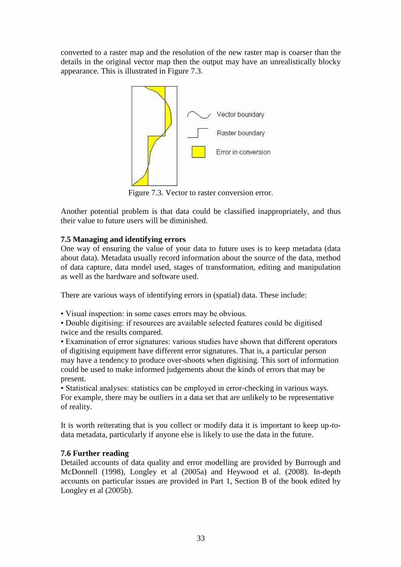
33
converted to a raster map and the resolution of the new raster map is coarser than the
details in the original vector map then the output may have an unrealistically blocky
appearance. This is illustrated in Figure 7.3.
Figure 7.3. Vector to raster conversion error.
Another potential problem is that data could be classified inappropriately, and thus
their value to future users will be diminished.
7.5 Managing and identifying errors
One way of ensuring the value of your data to future uses is to keep metadata (data
about data). Metadata usually record information about the source of the data, method
of data capture, data model used, stages of transformation, editing and manipulation
as well as the hardware and software used.
There are various ways of identifying errors in (spatial) data. These include:
• Visual inspection: in some cases errors may be obvious.
• Double digitising: if resources are available selected features could be digitised
twice and the results compared.
• Examination of error signatures: various studies have shown that different operators
of digitising equipment have different error signatures. That is, a particular person
may have a tendency to produce over-shoots when digitising. This sort of information
could be used to make informed judgements about the kinds of errors that may be
present.
• Statistical analyses: statistics can be employed in error-checking in various ways.
For example, there may be outliers in a data set that are unlikely to be representative
of reality.
It is worth reiterating that is you collect or modify data it is important to keep up-to-
data metadata, particularly if anyone else is likely to use the data in the future.
7.6 Further reading
Detailed accounts of data quality and error modelling are provided by Burrough and
McDonnell (1998), Longley et al (2005a) and Heywood et al. (2008). In-depth
accounts on particular issues are provided in Part 1, Section B of the book edited by
Longley et al (2005b).

34
Chapter 8. GIS project design, management and organization
8.1 Introduction
A GIS is only a worthwhile investment if it is set and used efficiently and effectively.
There are many stories of organisation investing time and money in technological
resources which are, ultimately, little used. This chapter outlines some factors that
should be considered during the set up and use of a GIS.
8.2 Setting up and implementing a GIS
Organisations establishing a GIS must consider several factors including:
• GIS applications: available software and hardware
• The needs of potential users
• Can investment in GIS be justified?
• Which system is appropriate and should it be implemented?
• What changes will GIS cause in an organisation?
(Source: Heywood et al., 2006)
One obvious way of assessing the more obvious potential problems and benefit is to
set up a pilot system. The design of a GIS requires various inputs. The design of the
software necessitates technical knowledge whereas the design of the system as a
whole (interaction of people and computers in an organisation). GIS system design
can be split into two parts: (i) technical design (internal) issues such as system design
and database; (ii) institutional design (external) issues including funding and technical
support (DeMers, 1999).
The way in which a GIS is set and its level of sophisticated will be largely a function
of the applications it is intended the GIS will be put. Applications of GIS can be
divided into three groups:
• Pioneering: high risk development of new applications. Either specialist
organisations or organisations with substantial financial resources.
• Opportunistic: taking advantage of the pioneer's work.
• Routine: use of a tried and tested product. Low risk strategy.
(Source: Heywood et al., 2006)
In most cases, the way in which GIS is used in an organisation will evolve. That is, as
users become aware of the functions available of the software their use of that
software is likely to expand with GIS becoming ever more central to the operation of
the organization concerned (Heywood et al., 2006).
8.3 Costs and benefits of a GIS
In setting up a GIS there will be costs relating to:
• Hardware and software
• Data
• Staff (including restructuring)

35
• Implementation study
Some of the key costs and benefits encountered in setting up a GIS are summarised in
Figure 8.1.
Figure 8.1. Summary of costs and benefits (after Obermeyer 2005, p. 609).
8.4 GIS project design
A key factor in the success of a GIS project is the design of the project. There are
various conceptual models and cartographic models than can be used to help design
an efficient, effective and flexible project plan. It is useful to develop a clear
schematic view of the stages which will be worked through during the project.
One approach to project design, System Life Cycle (SLC), consists of:
1. Feasibility study.
2. System investigation and system analysis.
3. System design.
4. Implementation, review and maintenance.
An alternative approach, prototyping, was developed in part as a response to the
limitations of SLC which is often considered overly structured and technocentric. The
prototyping approach has a greater emphasis on users and a prototype system is
introduced that can be adapted to meet the needs of users (Heywood et al., 2006).
8.5 Further reading
The book by Heywood et al (2006) and the chapter by Obermeyer (2005) informed
much of the account given in this chapter and they are good starting points for further
reading.
The next chapter outlines some of the applications within which GIS has been used.

36
Chapter 9. Applications of GIS
9.1 Introduction
There is a vast range of disciplines and organisations for whom GIS plays an
important role. Some examples include:
Agriculture Government
Archaeology Law enforcement
Banking and insurance Mining
Conservation Navigation
Defence Real Estate
Education Retail and commercial
Emergency services Site evaluation and planning
Engineering Telecommunications
Environmental management Transportation
Forestry Utilities
There are well-developed literatures concerned with all of these areas. This chapter
reviews applications in two different contexts through case studies. The first case
study is concerned with surveying an archaeological earthwork and generating maps
of its surface. The second case study deals with development of a coastal zone
management digital resource.
9.2 Case study 1: Generating a surface from point data
In this first case study a medieval earthwork (a rath) in Ballyhenry, Northern Ireland,
was surveyed using GPS. A surface was then generated from the point measurements
using interpolation. Figure 9.1 shows the locations of the positional measurements
made using GPS. Figure 9.2 shows a TIN derived from these point data while in
Figure 9.3 a 3D perspective of the same TIN is shown.

37
Figure 9.1. Locations of GPS positional measurements.
Figure 9.2. Shaded TIN derived from the point data in Figure 1.

38
Figure 9.3. '3D' view of shaded TIN derived from the point data in Figure 1.
When the archaeological site was surveyed it was due to be destroyed as it is within a
development area. As such, the digital representation is the most detailed record of an
archaeological feature which no longer exists.
Note that an introduction to GIS in archaeology is provided by Conolly and Lake
(2006).
9.3 Case study 2: Developing a multimedia coastal zone management resource
This case study outlines the contents and functions of the Down District Council
Coastal Zone Management Information System (DDCCZ MIS). The resource
contained a range of vector and raster data, the latter including photographs taken on
the ground that could be seen when certain sites were selected in the GIS.

39
Figure 9.4. The DDCCZ MIS.
The resource was intended to unify a range of data sources to aid in their
management. Figure 9.5 shows an example of the attribute data linked to vector
features. In Figure 9.6 a georeferenced aerial image is shown (that is, the image is
referenced using the same co-ordinate system as the vector data).

40
Figure 9.5. The linkage between vector spatial and attribute data.
Figure 9.6. A georeferenced remotely sensed image.

41
By unifying a diverse range of data sources such a resource can become a powerful
tool for a wide range of users, whether they wish to simply find out more about a
particular place or conduct detailed analyses of the spatial relations between different
spatial features.
9.4 Further reading
The best way of finding out about applications of GIS is to use an internet search
engine or look through recent volumes of academic journals like the International
Journal of Geographical Information Science (previously called International Journal
of Geographical Information Systems). Part 4 of the book edited by Longley et al.
(2005b) contains outlines of several applications areas and it is strongly
recommended.
A web search for GIS + any applications area is likely to result in many relevant hits.
In some contexts, terms such as ‘digital mapping’ may be preferred over GIS and this
should be considered when searching for material.
In the next, and final, chapter the concern is with recent developments in GIS and
how it may develop in the near future.

42
Chapter 10. GIS in the future
10.1 Introduction
This brief chapter focuses on some recent developments in GIS, but the main concern
is with some of the challenges ahead.
10.2 Problems and developments in GIS
The 1990s has seen extensive growth in the development, awareness and use of GIS.
In that decade, a major focus was on data input and huge GIS databases have been
developed from paper-based resources. GIS has become a key tool in the operations
of a wide range of organisations. In addition, the number of training courses has
proliferated.
Extensive digital datasets representing elements of both the physical and
socioeconomic environments are now available, and in many cases at no cost. With
the development of GIS software (and allied technologies such as Google Earth)
which can be freely downloaded, the capacity to visualise and manipulate digital
maps is limited only by access to computers and the internet. Free GIS environments
like GRASS GIS (http://grass.itc.it/) have extensive functionality and can be used to
implement the whole range of approaches detailed in this text.
Limitations in data structures (e.g., relational databases) and functionality have been
recognised and research continues to develop more intuitive models and more
powerful tools.
10.3 Where next for GIS?
There are several key areas in GIS which are likely to develop in the next decade.
Possible focuses concern:
• GIS type applications becoming ever more widely used (e.g., in spreadsheets, car
navigation etc).
• Virtual Reality enhancements.
• Enhancement of the role of GIS from decision support and problem solving to
generation of ideas and improvement of participation in decision support by all
players.
While the nature of specific developments are open to question it seems certain that
GIS is destined to grow further and to become an increasingly important component
(albeit hidden for many) in the lives of a large proportion of the world’s population.
10.4 Further reading
GIS is a rapidly changing field. Textbooks, such as those by Longley et al. (2005a)
and Heywood et al. (2006) can provide perspectives on developments up to the date
of publication, but these perspectives may become dated quickly.
Recent viewpoints are provided in the final chapters of the book edited by Wilson and
Fotheringham (2008). The internet and recent issues of academic journals, like the

43
International Journal of Geographical Information Science, are sensible starting
points in assessing the very latest developments.

44
References
Burrough, P. A. (1986) Principles of Geographical Information Systems for Land
Resources Assessment. Oxford: Oxford University Press.
Burrough, P. A. and McDonnell, R. A. (1998) Principles of Geographical
Information Systems. Oxford: Oxford University Press.
Chang, K. (2008) Introduction to Geographic Information Systems. Fourth Edition.
Boston: McGraw-Hill.
Chou, Y.-H. (1997) Exploring Spatial Analysis in Geographic Information Systems.
Albany: OnWord Press.
Codd, E. F. (1970) A relational model of data for large shared data banks.
Communications of the Association for Computing Machinery, 13, 377–387.
Conolly, J. and Lake, M. (2006) Geographical Information Systems for
Archaeologists. Cambridge: Cambridge University Press.
DeMers, M. N. (1999) Fundamentals of Geographic Information Systems. Second
Edition. New York, Wiley.
Heywood, I., Cornelius, S. and Carver, S. (2006) An Introduction to Geographical
Information Systems. Third Edition. Harlow: Pearson Education.
Lloyd, C. D. (2010) Spatial Data Analysis: An Introduction for GIS Users. Oxford:
Oxford University Press.
Longley, P. A., Goodchild, M. F., Maguire, D. J. and Rhind, D. W. (2005a)
Geographic Information Systems and Science. Second Edition. Chichester: Wiley.
Longley, P. A., Goodchild, M. F., Maguire, D. J. and Rhind, D. W. (2005b) (Eds.)
Geographical Information Systems: Principles, Techniques, Management and
Applications. Second Edition, abridged. Hoboken, NJ: Wiley.
Martin, D. (1996) Geographic Information Systems: Socioeconomic Applications.
Second Edition. London: Routledge.
Obermeyer, N. J. (2005) Measuring the benefits and costs of GIS. In Longley, P. A.,
Goodchild, M. F., Maguire, D. J. and Rhind, D. W. (Eds.) Geographical
Information Systems: Principles, Techniques, Management and Applications.
Second Edition, abridged. Hoboken, NJ: Wiley, pp. 601-610.
O’Sullivan, D. and Unwin, D. J. (2002) Geographic Information Analysis. Hoboken,
NJ: John Wiley and Sons.
Wilson, J. P and Fotheringham, A. S. (2008) (Eds.) The Handbook of Geographic
Information Science. Maldon, MA: Blackwell Publishing.
Worboys, M., and Duckman, M. (2004) GIS: A Computing Perspective. Second
Edition. Boca Raton, FL: CRC Press.
General resources
Academic journals
IEEE Transactions on Geoscience and Remote Sensing
International Journal of Geographical Information Science
Transactions in GIS

45
Web resources
Guide to Geographic Information Systems: http://www.esri.com/what-is-gis


