A short tutorial on using pRoloc for spatial proteomics data analysis Laurent Gatto * and Lisa M. Breckels April 16, 2015 Abstract This tutorial illustrates the usage of the pRoloc R package for the analysis and interpretation of spatial proteomics data. It walks the reader through the creation of MSnSet instances, that hold the quantitative proteomics data and meta-data and introduces several aspects of data analysis, including data visualisation and application of machine learning to predict protein localisation. Keywords : Bioinformatics, organelle proteomics, machine learning, visualisation * [email protected]1
Transcript
A short tutorial on using pRoloc for spatial proteomics dataanalysis
Laurent Gatto∗and Lisa M. Breckels
April 16, 2015
Abstract
This tutorial illustrates the usage of the pRoloc R package for the analysis and interpretation ofspatial proteomics data. It walks the reader through the creation of MSnSet instances, that holdthe quantitative proteomics data and meta-data and introduces several aspects of data analysis,including data visualisation and application of machine learning to predict protein localisation.
MSnbase and pRoloc are under active developed; current functionality is evolving and new features willbe added. This software is free and open-source software. If you use it, please support the project byciting it in publications:
Gatto L. and Lilley K.S. MSnbase - an R/Bioconductor package for isobaric tagged massspectrometry data visualization, processing and quantitation. Bioinformatics 28, 288-289(2011).
Gatto L, Breckels LM, Wieczorek S, Burger T, Lilley KS. Mass-spectrometry-based spatialproteomics data analysis using pRoloc and pRolocdata. Bioinformatics. 2014 Feb 5.
If you are using the phenoDisco function, please also cite
Breckels L.M., Gatto L., Christoforou A., Groen A.J., Kathryn Lilley K.S. and TrotterM.W. The effect of organelle discovery upon sub-cellular protein localisation. J Proteomics,S1874-3919(13)00094-8 (2013)
For an introduction to spatial proteomics data analysis:
Gatto L, Breckels LM, Burger T, Nightingale DJ, Groen AJ, Campbell C, Nikolovski N, Mul-vey CM, Christoforou A, Ferro M, Lilley KS. A foundation for reliable spatial proteomics dataanalysis. Mol Cell Proteomics. 2014 Aug;13(8):1937-52. doi:10.1074/mcp.M113.036350.
Questions and bugs
You are welcome to contact me directly about pRoloc . For bugs, typos, suggestions or other questions,please file an issue in our tracking system1 providing as much information as possible, a reproducibleexample and the output of sessionInfo().
If you wish to reach a broader audience for general questions about proteomics analysis using R, youmay want to use the Bioconductor support site: https://support.bioconductor.org/.
Spatial (or organelle) proteomics is the study of the localisation of proteins inside cells. The sub-cellular compartment can be organelles, i.e. structures defined by lipid bi-layers,macro-molecular as-semblies of proteins and nucleic acids or large protein complexes. In this document, we will focus onmass-spectrometry based approaches that assay a population of cells, as opposed as microscopy basedtechniques that monitor single cells, as the former is the primary concern of pRoloc , although thetechniques described below and the infrastructure in place could also be applied the processed imagedata. The typical experimental use-case for using pRoloc is a set of fractions, originating from a totalcell lysate. These fractions can originate from a continuous gradient, like in the LOPIT [1] or PCP [2]approaches, or can be discrete fractions. The content of the fractions is then identified and quantified(using labelled or un-labelled quantitation techniques). Using relative quantitation of known organelleresidents, termed organelle markers, organelle-specific profiles along the gradient are determined andnew residents are identified based on matching of these distribution profiles. See for example [3] andreferences therein for a detailed review on organelle proteomics.
It should be noted that large protein complexes, that are not necessarily separately enclosed within theirown lipid bi-layer, can be detected by such techniques, as long as a distinct profile can be defined acrossthe fractions.
1.2 About R and pRoloc
R [4] is a statistical programming language and interactive working environment. It can be expanded byso-called packages to confer new functionality to users. Many such packages have been developed forthe analysis of high-throughput biology, notably through the Bioconductor project [5]. Two packages areof particular interest here, namely MSnbase [6] and pRoloc . The former provides flexible infrastructureto store and manipulate quantitative proteomics data and the associated meta-data and the latterimplements specific algorithmic technologies to analyse organelle proteomics data.
Among the advantages of R are robust statistical procedures, good visualisation capabilities, excellentdocumentation, reproducible research2, power and flexibility of the R language and environment it-self and a rich environment for specialised functionality in many domains of bioinformatics: tools formany omics technologies, including proteomics, bio-statistics, gene ontology and biological pathwayanalysis, . . . Although there exists some specific graphical user interfaces (GUI), interaction with R isexecuted through a command line interface. While this mode of interaction might look alien to newusers, experience has proven that after a first steep learning curve, great results can be achieved by non-programmers. Furthermore, specific and general documentation is plenty and beginners and advancedcourse material are also widely available.
2The content of this document is compiled (the code is executed and its output, text and figures, is displayeddynamically) to generate the pdf file.
Once R is started, the first step to enable functionality of a specific packages is to load them using thelibrary function, as shown in the code chunk below:
> library("MSnbase")
> library("pRoloc")
> library("pRolocdata")
MSnbase implements the data containers that are used by pRoloc . pRolocdata is a data package thatsupplies several published organelle proteomics data sets.
As a final setup step, we set the default colour palette for some of our custom plotting functionality touse semi-transparent colours in the code chunk below (see ?setStockcol for details). This facilitatesvisualisation of overlapping points.
The data used in this tutorial has been published in [7]. The LOPIT technique [1] is used to lo-calise integral and associated membrane proteins in Drosophila melanogaster embryos. Briefly, embryoswere collected at 0 – 16 hours, homogenised and centrifuged to collect the supernatant, removingcell debris and nuclei. Membrane fractionation was performed on a iodixanol gradient and fractionswere quantified using iTRAQ isobaric tags [8] as follows: fractions 4/5, 114; fractions 12/13, 115;fraction 19, 116 and fraction 21, 117. Labelled peptides were then separated using cation exchangechromatography and analysed by LS-MS/MS on a QSTAR XL quadrupole-time-of-flight mass spectrom-eter (Applied Biosystems). The original localisation analysis was performed using partial least squarediscriminant analysis (PLS-DA). Relative quantitation data was retrieved from the supplementary filepr800866n si 004.xls3 and imported into R as described below. We will concentrate on the firstreplicate.
2.2 Importing and loading data
This section illustrates how to import data in comma-separated value (csv) format into an appropriateR data structure. The first section shows the original csv (comma separated values) spreadsheet, aspublished by the authors, and how one can read such a file into Rusing the read.csv function. Thisspreadsheet file is similar to the output of many quantitation software.
In the next section, we show 2 csv files containing a subset of the columns of original pr800866n si 004-rep1.csv
file and another short file, created manually, that will be used to create the appropriate R data.
The three first lines of the original spreadsheet, containing the data for replicate one, are illustratedbelow (using the function head). It contains 888 rows (proteins) and 16 columns, including proteinidentifiers, database accession numbers, gene symbols, reporter ion quantitation values, informationrelated to protein identification, . . .
There are several ways to create the desired R data object, termed MSnSet, that will be used toperform the actual sub-cellular localisation prediction. Here, we illustrate a method that uses separatespreadsheet files for quantitation data, feature meta-data and sample (fraction) meta-data and thereadMSnSet constructor function, that will hopefully be the most straightforward for new users.
> ## The quantitation data, from the original data
> f1 <- dir(system.file("extdata", package = "pRolocdata"),
fdataFile.csv containing meta-data for the 888 features (here proteins).
> head(fdataCsv, n=3)
FBgn ProteinID FlybaseSymbol NoPeptideIDs
1 FBgn0001104 CG10060 G-ialpha65A 3
2 FBgn0000044 CG10067 Act57B 5
3 FBgn0035720 CG10077 CG10077 5
MascotScore NoPeptidesQuantified PLSDA
1 179.86 1 PM
2 222.40 9 PM
3 219.65 3
pdataFile.csv containing samples (here fractions) meta-data. This simple file has been createdmanually.
> pdataCsv
sampleNames Fractions
1 X114 4/5
2 X115 12/13
3 X116 19
4 X117 21
A self-contained data structure, called MSnSet (defined in the MSnbase package) can now easily begenerated using the readMSnSet constructor, providing the respective csv file names shown above andspecifying that the data is comma-separated (with sep = ","). Below, we call that object tan2009r1and display its content.
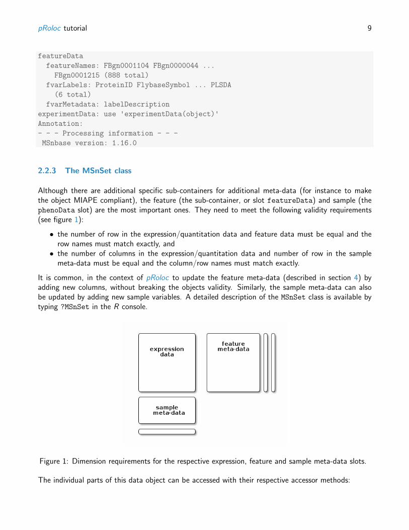
Although there are additional specific sub-containers for additional meta-data (for instance to makethe object MIAPE compliant), the feature (the sub-container, or slot featureData) and sample (thephenoData slot) are the most important ones. They need to meet the following validity requirements(see figure 1):
• the number of row in the expression/quantitation data and feature data must be equal and therow names must match exactly, and• the number of columns in the expression/quantitation data and number of row in the sample
meta-data must be equal and the column/row names must match exactly.
It is common, in the context of pRoloc to update the feature meta-data (described in section 4) byadding new columns, without breaking the objects validity. Similarly, the sample meta-data can alsobe updated by adding new sample variables. A detailed description of the MSnSet class is available bytyping ?MSnSet in the R console.
Figure 1: Dimension requirements for the respective expression, feature and sample meta-data slots.
The individual parts of this data object can be accessed with their respective accessor methods:
• the quantitation data can be retrieved with exprs(tan2009r1),• the feature meta-data with fData(tan2009r1) and• the sample meta-data with pData(tan2009r1).
The advantage of this structure is that it can be manipulated as a whole and the respective parts ofthe data object will remain compatible. The code chunk below, for example, shows how to extract thefirst 5 proteins and 2 first samples:
> smallTan <- tan2009r1[1:5, 1:2]
> dim(smallTan)
[1] 5 2
> exprs(smallTan)
X114 X115
FBgn0001104 0.379000 0.281000
FBgn0000044 0.420000 0.209667
FBgn0035720 0.187333 0.167333
FBgn0003731 0.247500 0.253000
FBgn0029506 0.216000 0.183000
Several data sets, including the 3 replicates from [7], are distributed as MSnSet instances in thepRolocdata package. Others include, among others, the Arabidopsis thaliana LOPIT data from [1](dunkley2006) and the mouse PCP data from [2] (foster2006). Each data set can be loaded withthe data function, as show below for the first replicate from [7].
> data(tan2009r1)
The original marker proteins are available as a feature meta-data variables called markers.orig andthe output of the partial least square discriminant analysis, applied in the original publication, in thePLSDA feature variable. The most up-to-date marker list for the experiment can be found in markers.This feature meta-data column can be added from a simple csv markers files using the addMarkers
function - see ?addMarkers for details.
The organelle markers are illustrated below using the convenience function getMarkers, but could alsobe done manually with table(fData(tan2009r1)$markers.orig) and table(fData(tan2009r1)$PLSDA)
Important As can be seen above, some proteins are labelled "unknown", defining non marker proteins.This is a convention in many pRoloc functions. Missing annotations (empty string) will not be consideredas of unknown localisation; we prefer to avoid empty strings and make the absence of known localisationexplicit by using the "unknown" tag. This information will be used to separate marker and non-markerproteins when proceeding with data visualisation and clustering (sections 3 and 4.1) and classificationanalysis (section 4.2.2).
2.3 pRoloc’s organelle markers
The pRoloc package distributes a set of markers that have been obtained by mining the pRolocdatadatasets and curation by various members of the Cambridge Centre for Proteomics. The availablemarker sets can be obtained and loaded using the pRolocmarkers functions:
These markers can then be added to a new MSnSet using the addMarkers function by matchingthe marker names (protein identifiers) and the feature names of the MSnSet. See ?addMarkers forexamples.
2.4 Data processing
The quantitation data obtained in the supplementary file is normalised to the sum of intensities of eachprotein; the sum of fraction quantitation for each protein equals 1 (considering rounding errors). Thiscan quickly be verified by computing the row sums of the expression data.
> summary(rowSums(exprs(tan2009r1)))
Min. 1st Qu. Median Mean 3rd Qu. Max.
0.9990 0.9999 1.0000 1.0000 1.0000 1.0010
The normalise method (also available as normalize) from the MSnbase package can be used toobtain relative quantitation data, as illustrated below on another iTRAQ test data set, available fromMSnbase. Several normalisation methods are available and described in ?normalise. For manyalgorithms, including classifiers in general and support vector machines in particular, it is importantto properly per-process the data. Centering and scaling of the data is also available with the scale
method, described in the scale manual.
In the code chunk below, we first create a test MSnSet instance4 and illustrate the effect of normalise(...,method = "sum").
iTRAQ4 quantification by trapezoidation: Thu Apr 16 21:15:48 2015
Normalised (sum): Thu Apr 16 21:15:48 2015
MSnbase version: 1.1.22
> head(exprs(itraqnorm), n = 3)
iTRAQ4.114 iTRAQ4.115 iTRAQ4.116 iTRAQ4.117
X1 0.08875373 0.1480074 0.2586772 0.5045617
X10 0.23178064 0.2503748 0.2232022 0.2946424
X11 0.23077081 0.2788287 0.2680598 0.2223407
> summary(rowSums(exprs(itraqnorm)))
Min. 1st Qu. Median Mean 3rd Qu. Max.
1 1 1 1 1 1
NA's
1
Note above how the processing undergone by the MSnSet instances itraqdata and itraqnorm isstored in another such specific sub-container, the processingData slot.
The different features (proteins in the tan2009r1 data above, but these could also represent peptidesor MS2 spectra) are characterised by unique names. These can be retrieved with the featureNames
function.
> head(featureNames(tan2009r1))
[1] "P20353" "P53501" "Q7KU78" "P04412" "Q7KJ73"
[6] "Q7JZN0"
If we look back at section 2.2.2, we see that these have been automatically assigned using the firstcolumns in the exprsFile.csv and fdataFile.csv files. It is thus crucial for these respective firstcolumns to be identical. Similarly, the sample names can be retrieved with sampleNames(tan2009r1).
The following sections will focus on two closely related aspects, data visualisation and data analysis(i.e. organelle assignments). Data visualisation is used in the context on quality control, to convinceourselves that the data displays the expected properties so that the output of further processing canbe trusted. Visualising results of the localisation prediction is also essential, to control the validity ofthese results, before proceeding with orthogonal (and often expensive) dry or wet validation.
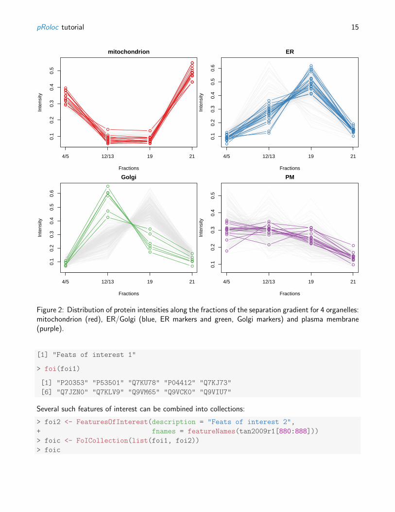
The underlying principle of gradient approaches is that we have separated organelles along the gradientand by doing so, generated organelle-specific protein distributions along the gradient fractions. Themost natural visualisation is shown on figure 2, obtained using the sub-setting functionality of MSnSetinstances and the plotDist function, as illustrated below.
i <- which(fData(tan2009r1)$PLSDA == "mitochondrion")
plotDist(tan2009r1[i, ],
markers = featureNames(tan2009r1)[j])
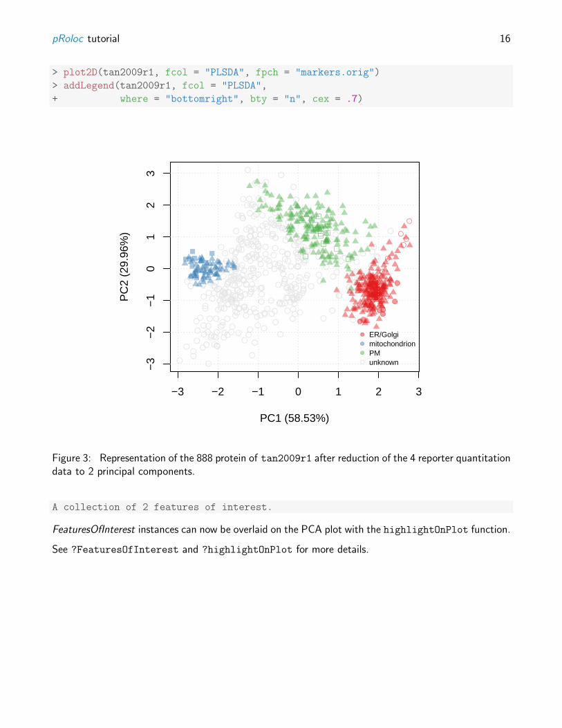
Alternatively, we can combine all organelle groups in one single 2 dimensional figure by applying adimensionality reduction technique such as Principal Component Analysis (PCA) using the plot2D
function (see figure 3). The protein profile vectors are summarised into 2 values that can be visualised intwo dimensions, so that the variability in the data will be maximised along the first principal component(PC1). The second principal component (PC2) is then chosen as to be orthogonal to PC1 whileexplaining as much variance in the data as possible, and so on for PC3, PC4, etc.
Using a PCA representation to visualise a spatial proteomics experiment, we can easily plot all theproteins on the same figure as well a many sub-cellular clusters (see figure 14 for a case with 11clusters). These clusters are defined in a feature meta-data column (slot featureData/fData) thatis declaraed with the fcol argument (default is "markers" which contains the most current knownmarkers for the experiment under investigation, the original markers published with the data can befound in the slot "markers.orig").
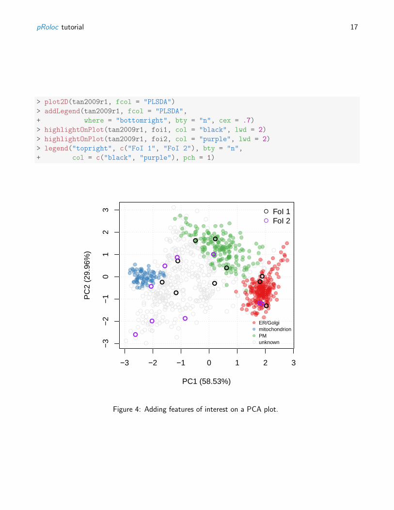
3.1 Features of interest
In addition to highlighting sub-cellular niches as coloured clusters on the PCA plot, it is also possible todefine some arbitrary features of interest that represent, for example, proteins of a particular pathwayor a set of interaction partners. Such sets of proteins are recorded as FeaturesOfInterest instances, asillstrated below (using the ten first features of our experiment):
> foi1 <- FeaturesOfInterest(description = "Feats of interest 1",
Figure 2: Distribution of protein intensities along the fractions of the separation gradient for 4 organelles:mitochondrion (red), ER/Golgi (blue, ER markers and green, Golgi markers) and plasma membrane(purple).
[1] "Feats of interest 1"
> foi(foi1)
[1] "P20353" "P53501" "Q7KU78" "P04412" "Q7KJ73"
[6] "Q7JZN0" "Q7KLV9" "Q9VM65" "Q9VCK0" "Q9VIU7"
Several such features of interest can be combined into collections:
> foi2 <- FeaturesOfInterest(description = "Feats of interest 2",
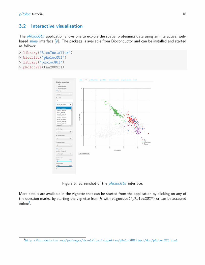
The pRolocGUI application allows one to explore the spatial proteomics data using an interactive, web-based shiny interface [9]. The package is available from Bioconductor and can be installed and startedas follows:
> library("BiocInstaller")
> biocLite("pRolocGUI")
> library("pRolocGUI")
> pRolocVis(tan2009r1)
Figure 5: Screenshot of the pRolocGUI interface.
More details are available in the vignette that can be started from the application by clicking on any ofthe question marks, by starting the vignette from R with vignette("pRolocGUI") or can be accessedonline5.
Classification of proteins, i.e. assigning sub-cellular localisation to proteins, is the main aspect of thepresent data analysis. The principle is the following and is, in its basic form, a 2 step process. First, analgorithm learns from the known markers that are shown to him and models the data space accordingly.This phase is also called the training phase. In the second phase, un-labelled proteins, i.e. those thathave not been labelled as resident of any organelle, are matched to the model and assigned to a group(an organelle). This 2 step process is called machine learning (ML), because the computer (machine)learns by itself how to recognise instances that possess certain characteristics and classifies them withouthuman intervention. That does however not mean that results can be trusted blindly.
In the above paragraph, we have defined what is called supervised ML, because the algorithm is presentedwith some know instances from which it learns (see section 4.2.2). Alternatively, un-supervised ML doesnot make any assumptions about the group memberships, and uses the structure of the data itself todefined sub-groups (see section 4.1). It is of course possible to classify data based on labelled andunlabelled data. This extension of the supervised classification problem described above is called semi-supervised learning. In this case, the training data consists of both labelled and unlabelled instanceswith the obvious goal of generating a better classifier than would be possible with the labelled dataonly. The phenoDisco algorithm, will be illustrated in that context (section 4.3).
4.1 Unsupervised ML
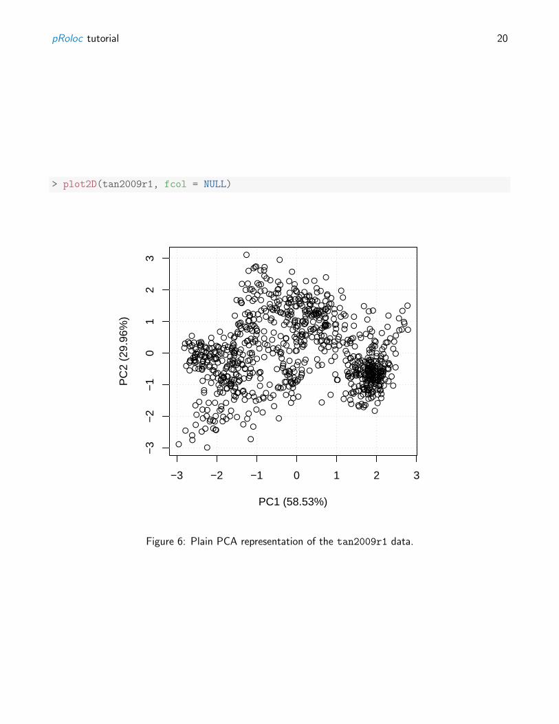
The plot2D can also be used to visualise the data on a PCA plot omitting any marker definitions, asshown on figure 6. This approach avoids any bias towards marker definitions and concentrate on thedata and its underlying structure itself.
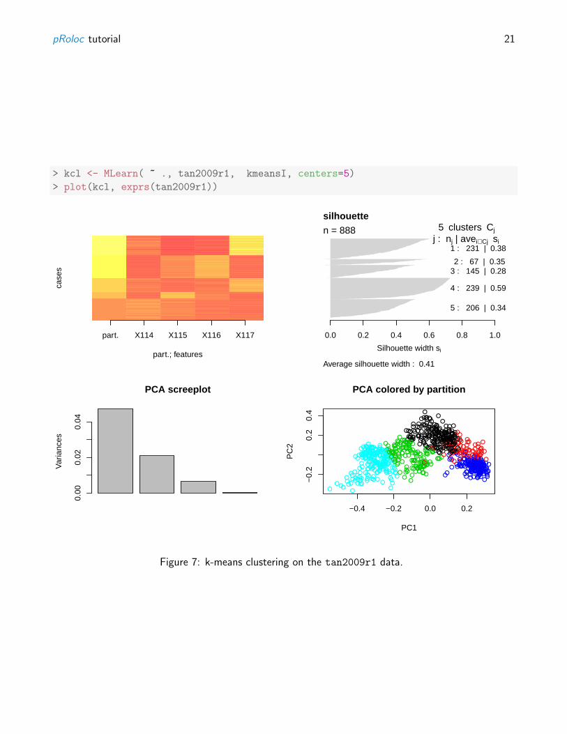
Alternatively, pRoloc also gives access to MLInterfaces’s MLean unified interface for, among others,unsupervised approaches using k-means (figure 7 on page 21), hierarchical (figure 8 on page 22) orpartitioning around medoids (figure 9 on page 23), clustering.
In this section, we show how to use pRoloc to run a typical supervised ML analysis. Several MLmethods are available, including k-nearest neighbour (knn), partial least square discriminant analysis(plsda), random forest (rf), support vector machines (svm), . . . The detailed description of each methodis outside of the scope of this document. We will use support vector machines to illustrate a typicalpipeline and the important points that should be paid attention to. These points are equally valid andwork, from a pRoloc user perspective, exactly the same for the other approaches.
Before actually generating a model on the new markers and classifying unknown residents, one has totake care of properly setting the model parameters. Wrongly set parameters can have a very negativeimpact on classification performance. To do so, we create testing (to model) and training (to predict)subsets using known residents. By comparing observed and expected classification prediction, we canassess how well a given model works using the macro F1 score (see below). This procedure is repeatedfor a range of possible model parameter values (this is called a grid search), and the best performingset of parameters is then used to construct a model on all markers and predict un-labelled proteins.
Model accuracy is evaluated using the F1 score, F1 = 2 precision×recallprecision+recall
, calculated as the harmonic
mean of the precision (precision = tptp+fp
, a measure of exactness – returned output is a relevant
result) and recall (recall = tptp+fn
, a measure of completeness – indicating how much was missed from
the output). What we are aiming for are high generalisation accuracy, i.e high F1, indicating that themarker proteins in the test data set are consistently correctly assigned by the algorithms.
In order to evaluate how well a classifier performs on profiles it was not exposed to during its creation,we implemented the following schema. Each set of marker protein profiles, i.e. labelled with knownorganelle association, are separated into training and test/validation partitions by sampling 80% ofthe profile corresponding to each organelle (i.e. stratified) without replacement to form the trainingpartition Str with the remainder becoming the test/validation partition Sts. The svm regularisationparameter C and Gaussian kernel width sigma are selected using a further round of stratified five-foldcross-validation on each training partition. All pairs of parameters (Ci, sigmaj) under considerationare assessed using the macro F1 score and the pair that produces the best performance is subsequentlyemployed in training a classifier on all training profiles Str prior to assessment on all test/validationprofiles Sts. This procedure is repeated N times (in the example below 10) in order to produce Nmacro F1 estimated generalisation performance values (figure 10). This procedure is implemented inthe svmOptimisation. See ?svmOptimisation for details, in particular the range of C and sigmaparameters and how the relevant feature variable is defined by the fcol parameters, which defaults to"markers". Note that here, we demonstrate the function with only perform 10 iterations6 (times =
10), which is enough for testing, but we recommend 100 (which is the default value) for a more robustanalysis.
6In the interest of time, the optimisation is not executed but loaded from dir(system.file("extdata", package
Figure 10: Assessing parameter optimisation. On the left, we see the respective distributions of the 10macro F1 scores for the best cost/sigma parameter pairs. See also the output of f1Count in relationto this plot. On the right, we see the averaged macro F1 scores, for the full range of parameter values.
In addition to the plots on figure 10, f1Count(params) returns, for each combination of parameters, thenumber of best (highest) F1 observations. One can use getParams to see the default set of parameters
that are chosen based on the executed optimisation. Currently, the first best set is automaticallyextracted, and users are advised to critically assess whether this is the most wise choice.
> f1Count(params)
0.5 1
0.1 1 0
1 NA 5
> getParams(params)
sigma cost
0.1 0.5
4.2.2 Classification
We can now re-use the result from our parameter optimisation (a best cost/sigma pair is going to beautomatically extracted, using the getParams method, although it is possible to set them manually),and use them to build a model with all the marker proteins and predict unknown residents using thesvmClassification function (see the manual page for more details). By default, the organelle markerswill be defined by the "markers" feature variables (and can be defined by the fcol parameter) e.g.here we use the original markers in "markers.orig" as a use case. New feature variables containingthe organelle assignments and assignment probabilities7, called scores hereafter, are automatically addedto the featureData slot; in this case, using the svm and svm.scores labels.
Added markers from 'mrk' marker vector. Thu Oct 30 18:21:04 2014
Performed svm prediction (sigma=0.1 cost=0.5) Thu Apr 16 21:15:50 2015
MSnbase version: 1.13.16
> tail(fvarLabels(svmres), 4)
[1] "markers.orig" "markers" "svm"
[4] "svm.scores"
The original markers, classification results and scores can be accessed with the fData accessor method,e.g. fData(svmres)$svm or fData(svmres)$svm.scores. Two helper functions, getMarkers and
7The calculation of the classification probabilities is dependent on the classification algorithm. These probabilities arenot to be compared across algorithms; they do not reflect any biologically relevant sub-cellular localisation probabilitybut rather an algorithm-specific classification confidence score.
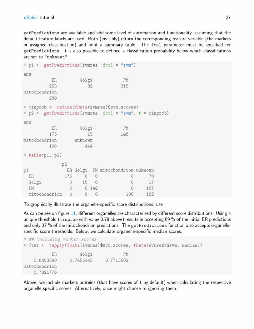
getPredictions are available and add some level of automation and functionality, assuming that thedefault feature labels are used. Both (invisibly) return the corresponding feature variable (the markersor assigned classification) and print a summary table. The fcol parameter must be specified forgetPredictions. It is also possible to defined a classification probability below which classificationsare set to "unknown".
> p1 <- getPredictions(svmres, fcol = "svm")
ans
ER Golgi PM
253 32 315
mitochondrion
288
> minprob <- median(fData(svmres)$svm.scores)
> p2 <- getPredictions(svmres, fcol = "svm", t = minprob)
ans
ER Golgi PM
175 15 148
mitochondrion unknown
106 444
> table(p1, p2)
p2
p1 ER Golgi PM mitochondrion unknown
ER 175 0 0 0 78
Golgi 0 15 0 0 17
PM 0 0 148 0 167
mitochondrion 0 0 0 106 182
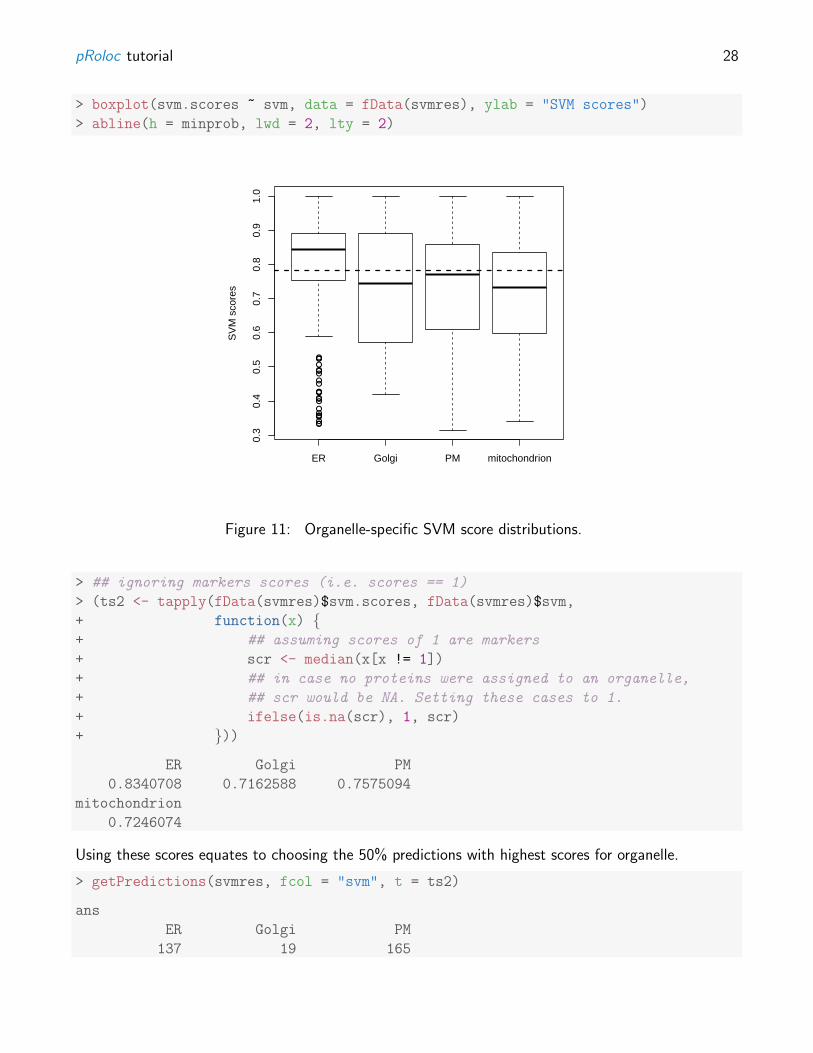
To graphically illustrate the organelle-specific score distributions, use
As can be see on figure 11, different organelles are characterised by different score distributions. Using aunique threshold (minprob with value 0.78 above) results in accepting 69 % of the initial ER predictionsand only 37 % of the mitochondrion predictions. The getPredictions function also accepts organelle-specific score thresholds. Below, we calculate organelle-specific median scores.
Above, we include markers proteins (that have scores of 1 by default) when calculating the respectiveorganelle-specific scores. Alternatively, once might choose to ignoring them.
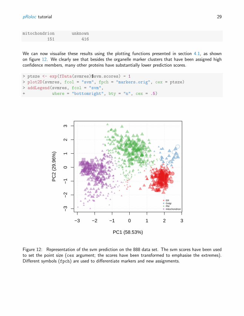
We can now visualise these results using the plotting functions presented in section 4.1, as shownon figure 12. We clearly see that besides the organelle marker clusters that have been assigned highconfidence members, many other proteins have substantially lower prediction scores.
Figure 12: Representation of the svm prediction on the 888 data set. The svm scores have been usedto set the point size (cex argument; the scores have been transformed to emphasise the extremes).Different symbols (fpch) are used to differentiate markers and new assignments.
It is obvious that the original set of markers initially used (ER, Golgi, mitochondrion, PM) is not abiologically realistic representation or the organelle diversity. Manually finding markers is however timeconsuming, as it requires careful verification of the annotation, and possibly critical for the subsequentanalysis, as markers are directly used in the training phase of the supervised ML approach.
As can be seen in the PCA plots above, there is inherent structure in the data that can be made useof to automate the detection of new clusters. The phenoDisco algorithm [10] is an iterative method,that combines classification of proteins to known groups and detection of new clusters. It is availablein pRoloc though the phenoDisco function8.
The results are also appended to the featureData slot.
> processingData(pdres)
- - - Processing information - - -
Combined [888,4] and [1,4] MSnSets Wed Feb 13 17:28:54 2013
Run phenoDisco using 'PLSDA': Wed Feb 13 17:28:54 2013
with parameters times=100, GS=10, p=0.05, r=1.
MSnbase version: 1.5.13
> tail(fvarLabels(pdres), 3)
[1] "PLSDA" "markers" "pd"
The plot2D function, can, as previously, be utilised to visualise the results, as shown on figure 13.
8In the interest of time, phenoDisco is not executed when the vignette is dynamically built. The data ob-ject can be located with dir(system.file("extdata", package = "pRoloc"), full.names = TRUE, pattern
The newly discovered phenotypes need to be carefully validated prior to further analysis. Indeed, as thestructure of the data is made use of in the discovery algorithm, some might represent peculiar structurein the data and not match with biologically relevant groups. The tan2009r1 data has been submittedto a careful phenodisco analysis and validation in [10]. The results of this new, augmented marker setis available in the pd.markers feature data. These markers represent a combined set of the originalmarkers and validated proteins from the new phenotypes.
> getMarkers(tan2009r1, fcol = "pd.markers")
organelleMarkers
Cytoskeleton ER Golgi
7 20 6
Lysosome Nucleus PM
8 20 15
Peroxisome Proteasome Ribosome 40S
4 11 14
Ribosome 60S mitochondrion unknown
25 14 744
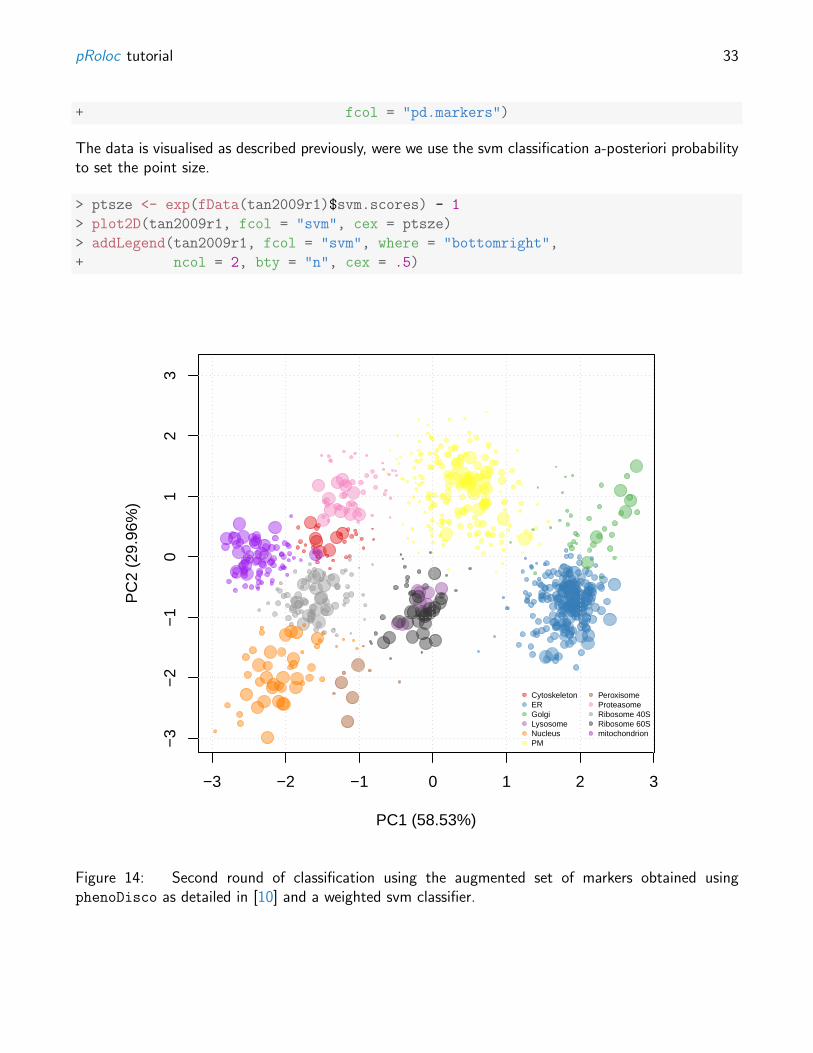
The augmented set of markers is now employed to repeat the classification using the support vectormachine classifier. We apply a slightly different analysis than described in section 4.2.2 (page 26). Inthe code chunks below9, we use class specific weights when creating the svm model; the weights areset to be inversely proportional to class frequencies.
Figure 14: Second round of classification using the augmented set of markers obtained usingphenoDisco as detailed in [10] and a weighted svm classifier.
This tutorial focuses on practical aspects of organelles proteomics data analysis using pRoloc . Twoimportant aspects have been illustrates: (1) data generation, manipulation and visualisation and (2)application of contemporary and novel machine learning techniques. Other crucial parts of a full analysispipeline that were not covered here are raw mass-spectrometry quality control, quantitation, post-analysis and data validation.
Data analysis is not a trivial task, and in general, one can not assume that any off-the-shelf algorithmwill perform well. As such, one of the emphasis of the software presented in this document is allowingusers to track data processing and critically evaluate the results.
We would like to thank Mr Daniel J.H. Nightingale, Dr Arnoud J. Groen, Dr Claire M. Mulvey and DrAndy Christoforou for their organelle marker contributions.
Session information
All software and respective versions used to produce this document are listed below.
• R version 3.2.0 (2015-04-16), x86_64-unknown-linux-gnu• Locale: LC_CTYPE=en_US.UTF-8, LC_NUMERIC=C, LC_TIME=en_US.UTF-8, LC_COLLATE=C,LC_MONETARY=en_US.UTF-8, LC_MESSAGES=en_US.UTF-8, LC_PAPER=en_US.UTF-8,LC_NAME=C, LC_ADDRESS=C, LC_TELEPHONE=C, LC_MEASUREMENT=en_US.UTF-8,LC_IDENTIFICATION=C
[1] Tom P. J. Dunkley, Svenja Hester, Ian P. Shadforth, John Runions, Thilo Weimar, Sally L. Hanton,Julian L. Griffin, Conrad Bessant, Federica Brandizzi, Chris Hawes, Rod B. Watson, Paul Dupree,and Kathryn S. Lilley. Mapping the arabidopsis organelle proteome. Proc Natl Acad Sci USA,103(17):6518–6523, Apr 2006. URL: http://dx.doi.org/10.1073/pnas.0506958103, doi:10.1073/pnas.0506958103.
[2] Leonard J. Foster, Carmen L. de Hoog, Yanling Zhang, Yong Zhang, Xiaohui Xie, Vamsi K.Mootha, and Matthias Mann. A mammalian organelle map by protein correlation profiling. Cell,125(1):187–199, Apr 2006. URL: http://dx.doi.org/10.1016/j.cell.2006.03.022, doi:10.1016/j.cell.2006.03.022.
[3] Laurent Gatto, Juan Antonio Vizcaıno, Henning Hermjakob, Wolfgang Huber, and Kathryn SLilley. Organelle proteomics experimental designs and analysis. Proteomics, 2010. doi:10.1002/pmic.201000244.
[4] R Development Core Team. R: A Language and Environment for Statistical Computing. RFoundation for Statistical Computing, Vienna, Austria, 2011. ISBN 3-900051-07-0. URL:http://www.R-project.org/.
[5] Robert C. Gentleman, Vincent J. Carey, Douglas M. Bates, Ben Bolstad, Marcel Dettling, SandrineDudoit, Byron Ellis, Laurent Gautier, Yongchao Ge, Jeff Gentry, Kurt Hornik, Torsten Hothorn,Wolfgang Huber, Stefano Iacus, Rafael Irizarry, Friedrich Leisch, Cheng Li, Martin Maechler,Anthony J. Rossini, Gunther Sawitzki, Colin Smith, Gordon Smyth, Luke Tierney, Jean Y. H.Yang, and Jianhua Zhang. Bioconductor: open software development for computational biol-ogy and bioinformatics. Genome Biol, 5(10):–80, 2004. URL: http://dx.doi.org/10.1186/gb-2004-5-10-r80, doi:10.1186/gb-2004-5-10-r80.
[6] Laurent Gatto and Kathryn S Lilley. MSnbase – an R/Bioconductor package for isobaric taggedmass spectrometry data visualization, processing and quantitation. Bioinformatics, 28(2):288–9,Jan 2012. doi:10.1093/bioinformatics/btr645.
[7] Denise J Tan, Heidi Dvinge, Andy Christoforou, Paul Bertone, Alfonso A Martinez, and Kathryn SLilley. Mapping organelle proteins and protein complexes in drosophila melanogaster. J ProteomeRes, 8(6):2667–78, Jun 2009. doi:10.1021/pr800866n.
[8] Philip L. Ross, Yulin N. Huang, Jason N. Marchese, Brian Williamson, Kenneth Parker, StephenHattan, Nikita Khainovski, Sasi Pillai, Subhakar Dey, Scott Daniels, Subhasish Purkayastha, PeterJuhasz, Stephen Martin, Michael Bartlet-Jones, Feng He, Allan Jacobson, and Darryl J. Pappin.Multiplexed protein quantitation in saccharomyces cerevisiae using amine-reactive isobaric taggingreagents. Mol Cell Proteomics, 3(12):1154–1169, Dec 2004. URL: http://dx.doi.org/10.
[9] RStudio and Inc. shiny: Web Application Framework for R, 2014. R package version 0.10.1. URL:http://CRAN.R-project.org/package=shiny.
[10] Lisa M Breckels, Laurent Gatto, Andy Christoforou, Arnoud J Groen, Kathryn S Lilley, and MatthewW B Trotter. The effect of organelle discovery upon sub-cellular protein localisation. J Proteomics,Mar 2013. doi:10.1016/j.jprot.2013.02.019.