A Simple Empirical Test for Equalizing Opportunities with an Application to Progresa * Jos´ e Luis Figueroa † Sherppa Dirk Van de gaer ‡ Sherppa and CORE June 1, 2015 Abstract We propose a simple test to establish whether a social program equalizes opportunities or not. The procedure is based on a comparison of the distribution of expected outcomes conditional on children’s circumstances when treated and when not treated. The procedure does not require the researcher to arbitrarily choose an inequality measure. It is applied to evaluate the effect of Progresa, the Mexican conditional cash transfer program, on inequality of opportunity for both school enrollment and passing to the next grade. Our findings are that Progresa partly compensates for unequal opportunities. 1 Introduction Social programs aim to alleviate poverty and increase opportunities for the vulnerable. The more a program succeeds in improving the opportunities for the most vulnerable, the more effective it is. Hence, in the evaluation of social programs, we are not only concerned with whether the program improves participating households’ outcomes like in the traditional literature on program evaluation, but we are also concerned with the distribution of the effects among households. It is well established that Progresa had positive effects on children’s school enrollment (see, e.g. Schultz (2004), Behrman et al (2005), Behrman et al (2011), Attanasio et al (2012) and Dubois et al (2012)), but much less is known about the distribution of enrollment effects among the children of participating households. In this paper, we are interested in the effect on the distribution of school enrollment and school performance between children facing different circumstances, where, as in the contributions by Bossert (1995), Fleurbaey (1995 and 2008) and Roemer (1993 and 1998), circumstances are defined as characteristics for which they are not * We thank Bart Cockx, Xavi Ramos, Ada Ferrer-i-Carbonell, Roxana Guti´ errez-Romero, Gerdie Everaert, Philippe Van Kerm, and Francesco Andreoli for useful comments and suggestions. We gratefully acknowledge comments received on preliminary versions presented at seminars at Universitat Aut`onoma de Barcelona, Ghent University, and University of Luxembourg. We acknowledge financial support from the FWO-Flanders, research project 3G079112. † SHERPPA, Vakgroep Sociale Economie, F.E.B., Ghent University, Sint-Pietersplein 6, B-9000 Gent, Belgium. ‡ SHERPPA, Vakgroep Sociale Economie, F.E.B., Ghent University, Sint-Pietersplein 6, B-9000 Gent, Belgium. and CORE, Universit´ e Catholique de Louvain, Voie du Roman Pays 34, B-1348 Louvain-la-Neuve, Belgium 1
Transcript
A Simple Empirical Test for Equalizing Opportunities
with an Application to Progresa ∗
Jose Luis Figueroa †
SherppaDirk Van de gaer ‡
Sherppa and CORE
June 1, 2015
Abstract
We propose a simple test to establish whether a social program equalizes opportunities or not. Theprocedure is based on a comparison of the distribution of expected outcomes conditional on children’scircumstances when treated and when not treated. The procedure does not require the researcherto arbitrarily choose an inequality measure. It is applied to evaluate the effect of Progresa, theMexican conditional cash transfer program, on inequality of opportunity for both school enrollmentand passing to the next grade. Our findings are that Progresa partly compensates for unequalopportunities.
1 Introduction
Social programs aim to alleviate poverty and increase opportunities for the vulnerable. The more aprogram succeeds in improving the opportunities for the most vulnerable, the more effective it is. Hence,in the evaluation of social programs, we are not only concerned with whether the program improvesparticipating households’ outcomes like in the traditional literature on program evaluation, but we arealso concerned with the distribution of the effects among households. It is well established that Progresahad positive effects on children’s school enrollment (see, e.g. Schultz (2004), Behrman et al (2005),Behrman et al (2011), Attanasio et al (2012) and Dubois et al (2012)), but much less is known about thedistribution of enrollment effects among the children of participating households. In this paper, we areinterested in the effect on the distribution of school enrollment and school performance between childrenfacing different circumstances, where, as in the contributions by Bossert (1995), Fleurbaey (1995 and2008) and Roemer (1993 and 1998), circumstances are defined as characteristics for which they are not
∗We thank Bart Cockx, Xavi Ramos, Ada Ferrer-i-Carbonell, Roxana Gutierrez-Romero, Gerdie Everaert, Philippe VanKerm, and Francesco Andreoli for useful comments and suggestions. We gratefully acknowledge comments received onpreliminary versions presented at seminars at Universitat Autonoma de Barcelona, Ghent University, and University ofLuxembourg. We acknowledge financial support from the FWO-Flanders, research project 3G079112.†SHERPPA, Vakgroep Sociale Economie, F.E.B., Ghent University, Sint-Pietersplein 6, B-9000 Gent, Belgium.‡SHERPPA, Vakgroep Sociale Economie, F.E.B., Ghent University, Sint-Pietersplein 6, B-9000 Gent, Belgium. and
CORE, Universite Catholique de Louvain, Voie du Roman Pays 34, B-1348 Louvain-la-Neuve, Belgium
1
held responsible, such as their sex, whether their parents are indigenous or not, the educational level oftheir parents or the state in which they live. Cappelen et al (2007) and Cappelen et al (2010) have shownthat for many people, when making distributional judgments, the distinction between factors beyondindividual control (i.e. circumstances) and within individual control matters. Moreover, Marrero andRodrıguez (2013), using data for the U.S. from the Panel Survey on Income Dynamics, find that incomeinequality which is accounted for by circumstances correlates negatively with growth. Hence we areinterested in the effect of Progresa on inequality of school enrollment and passing opportunities for bothnormative and positive reasons.
Following the work by Pistolesi (2009) and Ferreira and Gignoux (2011), a substantial part of therecent empirical literature measuring inequality of opportunity defines inequality of opportunity as theinequality in a counterfactual distribution in which all inequalities are due to differences in circumstances.To construct the latter, the outcome of interest is regressed upon a set of circumstances, and eachindividual is assigned the expected outcome calculated on the basis of his circumstances. Next, aninequality measure is chosen to compute the inequality in the distribution of these conditional expectedoutcomes. For a discussion of this and other approaches to the measurement of inequality of opportunitysee Ramos and Van de gaer (2012), for an application to the measurement of inequality of opportunityfor income see Marrero and Rodrıguez (2012).
In a previous paper (Figueroa and Van de gaer (2015)), we followed a similar approach to measure theeffect of Progresa on school enrollment the year after the program was initiated. We used the randomizedtreatment and control group used in much of the Progresa evaluation literature to estimate the effectof program participation and a list of circumstances on school enrollment. This allowed us to constructexpected school enrollment in the case the child’s household participated in Progresa, and in case thehousehold did not participate. We measured and compared the inequality in the resulting distributionsof expected outcomes with and without treatment by choosing as inequality measure the dissimilarityindex present in the Human Opportunity Index, proposed by Paes de Barros et al (2008 and 2009) andused by Molinas Vega et al (2012) and Foguel and Veloso (2014). We found that the value of this indexwas substantially lower in the distribution with than in the distribution without program participation.This suggested that Progresa reduced inequality of opportunities for school enrollment.
A disadvantage of this approach is that the results may be sensitive to the chosen inequality measure.In this paper, we propose an alternative and intuitively attractive way to evaluate a program’s effecton inequality of opportunity that does not display such a sensitivity. Figure 1 illustrates the intuition.The horizontal axis measures the value of the expected outcome conditional on circumstances in case thehousehold is not treated, H0, the vertical axis measures the value of the expected outcome conditionalon circumstances in case the household is treated, H1. Given a distribution of H0, the four lines in thefigure tell us how the treatment maps the distribution of H0 into a distribution of H1. The slope of thelines is given by α1 and determines the length of the interval into which all values of H0 that lie between,e.g.,
[h00, h
01
]will be mapped. Hence the slope determines the extent to which the treatment concentrates
or disperses the distribution of the expected outcomes after treatment. If α1 = 0, all elements of theinterval will be mapped into h10 such that the program eliminates the dispersion in expected outcomescompletely, if 0 < α1 < 1, they will be mapped into
[h10, h
11
]which is shorter than
[h00, h
01
], and the
program decreases the dispersion. If α1 = 1, they will be mapped in the interval[h10, h
12
]which is of the
same length as[h00, h
01
]such that the program has no effect on the dispersion. Clearly now, continuing
the argument, if α > 1 the program increases the dispersion of expected outcomes.
This motivates the following procedure to evaluate the effect on inequality of opportunity of a pro-gram. First, construct the expected value of the oucome of interest conditional on circumstances withouttreatment, H0 and with treatment, H1. Next, perform a simple regression of H1 on H0. If the cor-responding regression coefficient α1 is zero, the program fully equalizes opportunities, if it is betweenzero and one, the program partly equalizes opportunities, if it is one, it has no effect on inequality ofopportunity, while if it is larger than 1, it amplifies inequality of opportunity.
2
Figure 1: Intuitive idea of the test.
0 α 1
α = 1
α = 0
α 1
Notes: The figure illustrates how the slope of the regression of H1, the value of the expected outcome with treat-ment, on H0, the value of the expected outcome without treatment, determines the dispersion in the distributionof H1. As the slope of the regression, α1 increases, the probability mass in the interval
[h00, h
01
]will be spread
over a larger interval of values for H1.
To apply this simple idea, we first have to identify the effect of the program and of the child’scircumstances on the outcome. We are interested in being enrolled and in passing (which requires beingenrolled and proceeding to a higher grade next year). These outcomes are binary and we use a logisticregression to estimate the effect of the program and the child’s circumstances. The second step is toconstruct the expected outcomes. In our context, at first sight, it seems plausible to use the estimatedprobabilities to be enrolled (or to pass to the next grade). However, these probabilities are alwaysbetween zero and one, which would introduce a downward bias in the regression that is to be performedin the next step. To overcome this, we work with the inverse logits. The third step is then to regressthe inverse logit with program participation on the inverse logit without program participation and totest whether the regression coefficient is significantly different from zero or one. We present estimatesconditional on the grade completed at the start of the school year. All our estimates for Progresa arebetween zero and one, most are significantly smaller than one, and many are significantly different fromzero. Hence we conclude that Progresa partly equalizes opportunities for school enrollment between thechildren of families that benefit from the program.
Our simple test procedure is conditional on the linearity of the function mapping H0 into H1. Theintuition can be carried over to non linear specifications, however. In that case, the program declinesinequality of opportunity, if, over the support of H0, the slope of the non linear function that maps H0
into H1 is smaller than one, it partly compensates if the slope is between zero and one, and it increasesinequality of opportunity if the slope is larger than one.
There are two other applications of the recent literature on inequality of opportunity to projectevaluation. Both are inspired by Roemer (1993 and 1998). Van de gaer et al. (2014) determines theeffect of Oportunidades (former Progresa) on the distribution of children’s health outcomes, conditionalon their circumstances. It uses tests for restricted stochastic dominance developed by Davidson andDuclos (2013) to identify which children gain, but provides no overall assessment of the effect of theprogram on inequality of opportunity. The other application is Andreoli et al. (2014), which determinesthe effect of child care expansion in Norway on the distribution of their earnings 30 years later, conditionalon their parents’ earnings decile, using techniques of (inverse) stochastic dominance. By comparing theeffect of child care expansion on all possible pairwise conditional distributions, they establish that child
3
care expansion led to a decrease of inequality of opportunity. Both approaches rely on a comparisonof non-parametrically estimated conditional distribution functions, which makes them much harder toimplement than the test presented in the present paper, and limits the number of different values thatcircumstances can take: 4 in the case of Van de gaer el al. (2014), 10 in the case of Andreoli et al. (2014).With the parametric approach followed in this paper, circumstances can take on much more differentvalues.
The remainder of the paper is structured as follows. Section 2 provides a formal description of the testwe propose. Section 3 discusses Progresa, the way the data were selected and some simple descriptivestatistics of the sample we use. Section 4 gives the empirical results. The final Section concludes.
2 Formal Description
The first step in the procedure requires us to estimate the effect of the program and circumstanceson the outcome of interest, say school enrollment. As this outcome is binary, we estimate a standardlogistic regression. Define the inverse logit
Zi = β0 +
K∑k=1
βkXik + γ0Pi +
K∑k=1
γkPiXik, (1)
where the index i = 1, · · · , n denotes the identity of the child, Pi is a dummy variable indicating whetherthe child received treatment (Pi = 1) or not (Pi = 0) and Xik is the value of circumstance k for childi (k = 1, · · · ,K). It is important to include interaction effects between the treatment dummy andcircumstances in the specification, as these effects will determine whether the treatment compensates foror amplifies the effects of circumstances. Let Yi = 1 if the child is enrolled and Yi = 0 otherwise. Thestandard logistic specification is then
Prob(Yi = 1) =exp(Zi)
1 + exp(Zi). (2)
Standard logistic regression yields the 2(1 +K) dimensional vector [β′ γ′], containing the estimates of[β′ γ′]. These estimates are used in the next step.
The second step computes the inverse logits using the estimates of the first step. The value of theinverse logit in case the individual is (not) treated is H1
i , (H0i ), obtained from Equation (1) by putting
Pi = 1 (0), such that
H1i = β0 +
K∑k=1
βkXik + γ0 +
K∑k=1
γkXik, (3)
H0i = β0 +
K∑k=1
βkXik. (4)
The third step brings the estimates of (3) and (4) together in the n dimensional vectors H1 and H0,respectively. Our test is based on the slope coefficient estimate of the following simple regression:
H1 = α0 + α1H0 + U, (5)
4
where U is a n− dimensional vector of disturbance terms. The least square estimates of the coefficientsare given in the usual way, i.e.,
α0 =
∑ni=1H
1i
n− α1
∑ni=1H
0i
n, (6)
α1 =1n
∑ni=1(H0
iH1i ) − 1
n (∑ni=1H
0i ) 1n (∑ni=1H
1i )
1n
∑ni=1(H0
i )2 − ( 1n
∑ni=1H
0i )2
. (7)
It is easy to see that statistic (7) provides a test for the equalizing effect of the program. Suppose theprogram manages to fully equalize opportunities. In that case, for all i, H1
i = H, the same value foreveryone, and α1 = 0. If, by contrast, the program has no effect, then for all i, H1
i = H0i , and α1 = 1.
Observe that the regression coefficients α0 and α1 depend on the estimated H0i and H1
i , which
depend on the estimated coefficient estimates x′ = [β′ γ′] - see (3) and (4). Therefore, the estimatedstandard errors of the regression coefficients can be found using the delta method. More in particular, letΩx ≡ Ωβγ be the estimated 2(1 +K) dimensional variance covariance matrix of the coefficient estimates.We can then show that the statistic α1 is a consistent estimator of its population counterpart. It isasymptotically normally distributed and its asymptotic variance can be estimated by
σ2(α1) =∂α1
∂x′Ωx
∂α1
∂x.
Having obtained the estimate α1 and its estimated (asymptotic) standard errors, it is straightforward totest in the fourth and final step whether α1 is significantly larger than zero and smaller than one.
3 Data
Progresa is the predecessor of the Oportunidades program, which turned into Prospera in 2014,the main anti-poverty program of the Mexican government today. Its main purposes are to alleviateimmediate poverty and break the intergenerational poverty cycle. The program gives in-kind healthbenefits, including nutritional supplements for children up to ages five and for pregnant and lactatingwomen, as well as monetary transfers. These cash transfers consist out of grants for consumptionof food, conditional on attending scheduled visits to health centers at the one hand, and educationalgrants, conditional on attending school at least 85% of the time on the other hand. Parents receivemoney for school materials per child, and, from grade 3 in primary school onwards, an educational grantthat increases as children advance in school (reflecting increasing opportunity costs). To induce familiesto keep girls longer in school, grants are higher for girls than for boys from secondary school onwards.
Households that experienced extreme poverty and lived in highly deprived rural localities with accessto a primary school and a health clinic were included in the program. A random procedure assignedlocalities to receive treatment in May 1998; the other localities received treatment from early 2000onwards. We use data that were collected in October 1998 and November 1999, when the households inthe immediate treatment localities already received treatment, but not the delayed treatment localities,which, following much of the literature (e.g. Gertler (2004), Schultz (2005), Behrman et al (2005), Toddand Wolpin (2006), Attanasio et al (2012), Dubois et al (2012)), serve as our control group. Data werecollected in 320 treatment and 186 control localities. An excellent further discussion of Progresa and theconstruction of evaluation samples can be found in Skoufias (2005).
Our data set is based on the information of all children aged 6-16 that lived in interviewed house-holds experiencing extreme poverty in one of the 360 treatment or 186 control localities. As the grants
5
households receive depend on the grade level the child is in, we perform the logistic regression for eachsubsample containing the children that have obtained the same grade level (0 to 9) at the start of theschool year in August 1998. This information was present in the data set for 95% of the children. As wealso focus on passing, we also need information on the grade obtained at the end of the school year; wehad this information for 94.6% of the children for which we observed the grade at the start of the schoolyear. The combination of these data allow us to see whether children progressed. We noticed that somechildren have negative progress and others progressed an implausibly large number of years. To deal withthis issue, we impose a further sample restriction. As it is not uncommon in the rural part of Mexico forolder children to start school at a grade below their age, and jump the next year one or two grades (seeBehrman et al. (2005), page 242), our sample contains those children that progressed between 0 and 3years (containing 86.6% of the children for which we observe both grades). In the sensitivity analysis, werepeat the whole analysis for the sample of those children that progress between 0 and 1 year (containing69% of the children for which we observe both grades). Table 1 provides a comparison of the core datafor the sample used in the main analysis.
Table 1: Comparison of treatment and control group
Grade # Obs % Enrolled TS % Passing TS % Passing ES1998 T C T C T C T C
Notes: “% Enrolled TS” stands for “the percentage enrolled of the totalsample”, “ % Passing TS (ES)” stands for “the percentage that passed of thetotal (enrolled) sample”. “T” (“C”) refers to the treatment (control) group.
School enrollment rates are high for all grades, except for those that completed grades 6 and 9. Havingcompleted grade 6, primary education is finished, and many children quit school. The same happens forthose that complete grade 9, that is for those that completed secondary education. We follow Schultz(2004, page 205) and consider that the conditionality of the size of the educational grant on grade andthe large discontinuities in enrollment rates on the basis of grades provides a justification to estimate thelogistic model for each grade obtained at the beginning of the school year rather than age. Enrollmentrates in the treatment group (column 4) are only slightly higher than in the control group (column 5),except for those having completed grades 6 and 9. Finally, for higher grades, passing in the treatmentgroup is lower as a percentage of the total sample (from grade 7 onwards) and as a percentage of theenrolled sample (from grade 3 onwards) than in the control group. Simple as they are, the results in thisTable are much in line with the conclusion from Dubois et el. (2012, p.588): “We find that Progresa hada positive impact on school continuation at all grade levels, whereas for performance (meaning passing)it had a positive impact at the primary school level but a negative effect at secondary school level.”Following the suggestion by Behrman et al (2011, p. 100), this could be due to a change in the selectionprocess into grades caused by the program: if the program induces children with lower scholarly abilityto stay in school, school enrollment can increase while passing decreases.
To measure the effect of the program on inequality of opportunity we have to select the circumstances,which are the characteristics for which children are not held responsible. This choice is based on normativeprinciples and data availability. We follow the literature on inequality of opportunity, and choose ascircumstances the child’s gender, its indigenous background, the gender of the household head, whether
6
the household head had a partner, whether a secondary school was present in the locality where thechild lives, the education level of both the household head and his spouse (no education, incompleteprimary education, or more than primary education) and the household’s state of residence (Veracruz,Guerrero, Hidalgo, Michoacan, Puebla, Queretaro or San Luis Potosı). Several of these circumstanceshave been used before, e.g., by Bourguignon et al. (2007), Ferreira and Gignoux (2011), Marrero andRodrıguez (2012) and Van de gaer et el. (2014). We include dummy variables that indicate which (ifany) of the other circumstances are missing because we did not want to loose the information that ispresent in those observations for which we miss information about some circumstances (across all grades,we miss observations on at least one circumstance for about 30% of the observations). In the sensitivityanalysis we show that leaving out the observations with missing circumstances does not affect out mainconclusions.
4 Results
Our logistic regression approach based on equations (1) and (2) identifies the effect of Progresa bycomparing children living in households that are treated with children living in households that are nottreated. This yields a correct estimate of the treatment effect only if the treated and control sample aresimilar in terms of pre-program characteristics. We tested for this in two ways. First, we compared, foreach grade, the composition of the treatment an control sample in terms of 41 pre-program characteristics(household assets and demographic variables) that are not used in the estimation of (1) and (2). Forgrades 5, 7 and 8, the samples differred in 1 characteristic, for grade 6 in 4, and for all the other gradesin 2. Second, we performed a logistic regression, regressing being in the treatment sample on the child’scircumstances and the same list of 41 pre-program characteristics. The number of coefficients of thelatter variables that influence the probability of being in the treatment sample significantly at a level offive percent, is 2 for 5 grades out of 10, and is always between 5(for grade 5) and 0 (for grade 3). Theseresults are encouraging. Hence we can follow the literature and assume that the treatment and controlsample are comparable (see, e.g. Behrman and Todd (1999)).
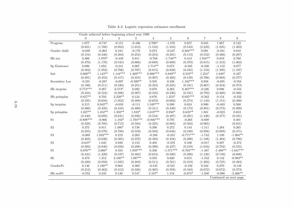
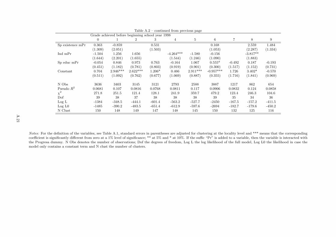
The logistic regressions for school enrollment and passing are found in Appendix A. The coefficientestimates in Table A2 imply a higher school enrollment for indigenous than for non indigenous children,and for children from better educated parents. The results for grade 6 show that, for this grade level, beinga boy and living in a locality with a secondary school significantly influence the probability of staying atschool after completing primary education. Some interaction dummies with Progresa participation arestatistically significant, especially those with being indigenous and the household’s state of residence.Only in 16 cases are both the effect of a circumstance and its interaction effect with Progresa estimatedto be significantly different from zero at 10%. However, in 14 out of those 16 cases, the absolute value ofthe sum of the coefficient and its interaction effect is smaller than the absolute value of the coefficient.This is a first piece of evidence indicating that Progresa might compensate for some of the effects ofcircumstances. The results for passing, reported in Table A.3, are somewhat different. Fewer coefficientsare statistically significant from zero and the explanatory power of the regression is lower. There isstill some, albeit weaker evidence for children from better educated parents to have a higher probabilityof passing, but being indigenous is not associated with passing. The presence of a secondary schoolin the locality is associated passing in grade 6, being a boy is associated with less passing in grade 7.The Progresa dummy is significantly negative for grade 7. Only in 10 cases are both the effect of acircumstance and its interaction effect with Progresa estimated to be significantly different from zeroat 10%. This time in 9 out of those 10 cases, the absolute value of the sum of the coefficient and itsinteraction effect is smaller than the absolute value of the coefficient, such that also here there is someweak evidence that Progresa might compensate for the effect of circumstances.
Table 2 compares the distributions of the inverse logits in case the household participates in Progresa(H1) and in case it does not participate (H0), for both, school enrollment (Panel A) and passing (PanelB).
Notes: Columns 2 gives the average value of the inverse logit forenrollment (panel A) and passing (panel B) when households par-ticipate in Progresa; column 3 gives the average value of the inverselogit when households do not participate in Progresa; column 4 givesthe percentage of households for which the value of the inverse logitwhen it participates in Progresa is larger than when it does not par-ticipate. Column 5 provides the rank correlation between H1 andH0; in all cases, the null for H1 and H0 independent was rejected at1% level of significance. Column 6 and 7 provide the variance of H1
and H0, respectively.
The results in this Table largely confirm those from descriptive Table 1. The program increases theaverage value of the inverse logits for school enrollment for most grades (grade 7 is the largest exception).The largest positive effect on the inverse logit occurs for those having completed primary school (grade6), with also a very high percentage of children predicted to see an increase in school enrollment. Thisis in line with Schultz (2004). Looking at the inverse logits for passing, the predicted effects of theprogram, measured by the percentage of children predicted to see their probability of passing, increaseddue to the program are smaller than for school enrollment. Again the largest positive effect is found forgrade 6, but for grade 7 and 8 program participation seems to be associated with less passing. Column 5shows that the rank correlation between H0 is about 0.5 on average, and is always positive. Comparisonof Columns 6 and 7 shows that the variance of the inverse logit when households participate is almostalways smaller then when the household does not participate. The only excpetions are grade 5 for schoolenrollment and grade 0 for passing.
We pointed out in the introduction that our simple test is conditional on the linearity of the specifi-cation in (5). We tested for the linearity by including a quadratic term in (5). The results can be foundin Table B.1. The coefficient of the quadratic term was never significantly different from zero. Hence weproceed with our simple test.
8
Table 3 provides the results from our formal test. It reports the estimates of the coefficients α0 and α1
and their standard errors for each grade level obtained at the start of the school year 1998-99. Rememberthat for our test to be a valid test of equality of opportunity, all differences in H1 and H0 in Equation(5) must be entirely due to differences in circumstances. This explains why we do not pool all gradesin one regression, as that would imply that differences in grades attained are treated as circumstances,which can be questioned.
For both school enrollment and passing, all the estimated values of α1 are between zero and one.In most cases, they are significantly smaller than one, and in many cases they are also significantlypositive. The former indicates that Progresa equalizes opportunities, the latter that the equalization isnot complete. Hence, the estimates transmit a clear message: Progresa manages to partly compensatechildren for their circumstances, but the compensation is far from complete, especially in the crucialgrade 6, where the estimated value for α1 is 0.7 for school enrollment and 0.578 for passing. Two furtherobservations can be made. First, the estimated coefficients are also between zero and one for childrenthat did not qualify for school subsidies because they were not in grade 3 at the start of the schoolyear since they completed less than 2 grades at that point. However, enrollment of these children isstimulated by the program, as this is the best strategy to ensure that they will, in the near future,complete grade 2 and the family qualifies for the educational grant. Moreover, these children can benefitfrom Progresa’s consumption grants, educational grants received for older siblings and health check ups,and these benefits might have larger impacts for children from disadvantaged households. Second, forchildren that completed less than 5 grades and for those that completed 9 grades, the estimated coefficientfor school enrollment is smaller than for passing, though the difference is not statistically significant.
9
Table 3: Test for the effect on inequality of opportunity
Notes: The table reports, for each grade, the results for both enrollment (columns 2 to 6) and passing(columns 7 to 11). α1 (α0) is the estimated value of the slope (intercept) of the regression of the predictedvalue of the inverse logit when treated on its value when not treated. Standard errors for these estimatesare based on the delta method and are given in parenthesis below their estimated value. The columnslabelled α1 < 0 test the hypothesis that the slope is negative; the columns labelelled α1 > 1 test thehypothesis that the slope is larger than one. *** means that the hypothesis is rejected at a 1% level ofsignificance; ** at 5% and * at 10%.
10
We test the sensitivity of our results using different samples and sets of circumstances. First, observethat in Table 3, inequalities that are due to missing data are treated as a circumstance. It is not clearwhether this is legitimate, therefor, in Table B.2, we restrict the sample to those children for which noneof the data on these characteristics were missing. None of our conclusions is affected. Second, leastsquares regressions can be sensitive to outliers. To see whether our results suffer from such a sensitivity,for each grade obtained, we dropped those observations for which the estimated value of H0
i or H1i
belonged to the top or bottom 2.5% of the observations for that grade from the sample. The resultsare reported in Table B.3. Again, none of our conclusions is affected. Third, one might suspect thatthe results of our test are sensitive to the choice of circumstances. To see whether this is the case, werepeated the entire analysis without the household state of residence as a circumstance; we estimated thelogistic regressions without this variable, computed the corresponding inverse logits and ran regression(5). The results are given in Table B4. All estimates of α1 are positive (except one which is negativebut not significantly different from 0) and smaller than 1. Most are statistically significant positive andsmaller than 1. None of our conclusions is affected. Fourth, the sample for the analysis in the mainpart of the text included those children that progressed between 0 and 3 years. Table B.5 contains theresults when the sample includes only those children that progressed between 0 and 1 years. Again, allconclusion hold true.
Another important caveat for our simple test is the stochastic nature of H0i and H1
i , since bothdepend on the logistic coefficient estimates obtained in (3) and (4). This implies that both, H0
i and H1i ,
are measured with error, which in turn, introduces a downward bias in our linear estimate α1. In ourcase is possible to correct for such bias since we know the distribution of x′ = [β′ γ′]. Such correctionis usually based on asymptotic theory, therefore, we implement a Monte Carlo procedure to obtain thedistribution of the new (corrected) α1. The results are shown in Table 4. As can be observed from thelast two columns in the table, the results are less outspoken now: only in two cases the value 1 and 0are not contained in the 95% confidence interval (grades 0 and 6). However, our main result, namely theprogram partially equalizes opportunities for grade 6, remains.
Table 4: Distribution of estimates based on Monte Carlo
Panel A. EnrollmentGrade Av. α1 Med.α1 C.I. 95% Av. adj. α1 Med. adj. α1 C.I. 95%
Notes: In both panels, Columns 2 and 6 show the average value of α1 and the adjusted value ofα1 respectively; Columns 3 and 7 give the media of α1 and the media of adjusted α1 respectively;Columns 4-5 and 8-9 show the 95% confidence interval for α1 and the adjusted α1, respectively.
11
A final comment on the simple test procedure is in order. We have established that Progresa equalizesthe distribution of the inverse logits. It might be objected that inverse logits are not easy to grasp.Probabilities might be a more natural concept to look at. The linear specification in (5) implies anon linear mapping from the expected probability of enrollment without the program (say P 0) into theexpected probability with the program (say P 1). To investigate these issues, Tables B.6 and B.7 lookat the non linear mapping from the probabilities P 0 into P 1 implied by our estimates of the linearspecification in (5) for the probabilities of enrollment and passing, respectively. More in particular, foreach grade we computed which fraction of the observations are in the part of the support of P0 where theslope of the non linear mapping is between zero and one. This fraction is lowest for school enrollment ingrade 7, but even then it equals 70%. The second lowest fraction is for school enrollment in grade 2; hereit is 82%. For passing the lowest fraction is in grade 9 and is 86%. For all other grades, it is well above90%. This suggests that Progresa also equalized probabilities for school enrollment as well as passing.
Based on this evidence, it is clear that Progresa equalized opportunities. This is an important finding,but it also raises the question whether Progresa managed to compensate for all circumstances to thesame extent. In order to get a tentative answer to this question, we compared the contributions eachcircumstance to the variance of the distributions of H0 and H1, for both school enrollment and passingin the crucial grade 6, when the transition from primary to secondary school occurs and many childrenquit school. These results have to be interpreted with care as they depend on the use of the variance asinequality measure, and on the list of circumstances that are included.
Two circumstances contribute significantly to all variances: parental schooling, with children frombetter educated parents having better enrollment rates, and state of residence, with children residingin some states like, e.g., Guerrero having worse enrollment rates. Parental schooling is generally moreimportant than state of residence. Together they account for between 46 (Enrollment, H0) and 70%(Passing, H1) of the variances. For enrollment, the presence of a secondary school in the locality wherethe family lives and the indigenous background (only for H0) are also significant. For school enrollmentwithout treatment, the presence of a secondary school in the locality is even the most important cir-cumstance. Overall, the standard errors of the contributions are large, and this explains why we do notfind any significant differences between the contributions in the second and third, or the fourth and fifthcolumns. Nevertheless, for school enrollment, comparing the second and third column, it is striking thatthe program decreases the relative importance of the presence of a secondary school in the locality, andincreases the relative importance of parental background, especially the contribution of the school levelof the spouse. This suggests that, in order to decrease inequality of opportunity for school enrollmentfurther, special attention should go to children from lowly educated parents. For passing, comparingthe third and the fourth column, the program decreases the relative importance of the presence of asecondary school in the locality and increases the relative importance of the existence of the spouse, butstandard errors are huge and not much else is happening here. This is probably due to the lower fit ofthe passing logistic regression, and the larger standard errors of the estimated coefficients used in thecomputation of the inverse logits.
12
Table 5: Contributions of circumstances to the variance in counterfactuals(grade 6)
Notes: Columns labeled H0 refer to the inverse logits without treatment;columns labeled H1 refer to the inverse logits with treatment.
5 Conclusion
The distributional effects of social programs are important. The recent literature on the measurementof inequality of opportunity measures inequality of opportunity as the inequality in a (counterfactual)distribution where all inequality is due to circumstances only. We use this insight and propose to estimatefor each child ite expected outcome, given its circumstances, in case its household participates and incase its household does not participates. Our simple test for the equalizing opportunity effect of theprogram is based on a simple regression of the former on the latter, and does not require the choice of aparticular inequality measure.
Our results show that, the school year after Progresa was initiated, Progresa partially equalizedopportunities for school enrollment and passing enrollment within the group of households qualifyingfor the program (i.e. within the group of poor households living in poor localities) to a significantextent, without, however, fully equalizing them. These results are robust. It does not matter whetherthe sample is restricted to those children that progress between 0-1 years instead of 0-3 years, whetherthe household state of residence is treated as a circumstance or not, whether, in the test regression thesample is restricted to those without missing circumstances, or whether this sample is trimmed to excludepotential outliers. It is well known that Progresa had a big effect on school enrollment, especially forthose that completed primary education (grade 6). Our results point out that, for this grade level, theprogram also equalized opportunities for school enrollment, albeit to a lesser extent than for most othergrades.
In order to get an indication of the circumstances for which Progresa manages to compensate, wecomputed the relative contribution of the different circumstances to the variance of the counterfactuals
13
in grade 6. Parental schooling level is the most important circumstance, followed by household state ofresidence. The presence of a secondary school in the locality where the household lives is also important,especially for school enrollment, but Progresa decreases its relative importance. For school enrollment,this decrease is compensated by an increase in the relative importance of parental schooling, for pass-ing, it is compensated by an increase in the relative importance of the existence of the spouse. Whilethe decomposition results should be interpreted with care (they are based on the variance as inequal-ity measure, are sensitive to which circumstances are included and our estimated standard errors aresubstantial), they seem to suggest that to improve the effect of Progresa on inequality of opportunityfurther, special attention should be focused on children with lowly educated parents, and growing up indisadvantaged states like Guerrero. What form this special attention should take cannot be determinedon the basis of the present study. This requires either a structural equation model like the ones developedby Todd and Wolpin (2006) or Attanasio et al. (2012), or an in-depth analysis of why these childrenhave difficulties to be enrolled and pass.
The results we presented leave several other questions unanswered too. First, whether Progresaequalized school enrollment opportunities for all children in Mexico depends on the way it is financedand the effect this has on the opportunities of children living in families that do not participate inProgresa. Second, we evaluate the effects on school enrollment the first year Progresa existed. Whilethe methodology can be readily extended to evaluate longer run effects of the program, this is notstraightforward in the case of Progresa, because the households in the control group started receivingtreatment a few months after the first school year ended. Using the techniques used in Behrman etal. (2011) to estimate the long-run effects of the program and to construct the corresponding expectedoutcomes, the test developed here can readily be applied. Third, we abstract from the general equilibriumeffects of the program. Again, the test we propose can easily accommodate this, provided the expectedoutcomes are constructed in such a way that they incorporate general equilibrium effects. The approachused in Debowicz and Golan (2014) links micro- and macrosimulation models and can be used to do this.
14
References
Andreoli, F., T. Havnes and A. Lefranc (2014), Equalization of Opportunity: Definitions, ImplementableConditions and Application to Early-Childhood Policy Evaluation, IZA DP No. 8503.
Attanasio, O.P, C. Meghir and A. Santiago (2012), Educational Choices in Mexico: Using a StructuralModel and a Randomized Experiment to Evaluate PROGRESA, Review of Economic Studies 79, 37-66.
Behrman, J., and P.E. Todd (1999), Randomness in the Experimental Samples of PROGRESA Educa-tion, Health, and Nutrition Program. International Food Policy Research Institute.
Behrman, J., P. Sengupta and P.E. Todd (2005), Progressing through Progresa: an Impact Assessmentof a School Subsidy Experiment in Mexico. Economic Development and Cultural Change 54, 237-275.
Behrman, J., S.W. Parker and P.E. Todd (2011), Do Conditional Cash Transfers for Schooling GenerateLasting Benefits? Journal of Human Resources 46, 93-122.
Bossert, W. (1995), Redistribution mechanisms based on individual characteristics. Mathematical SocialSciences 29, 1-17.
Bourguignon, F., F.H.G. Ferreira and M. Menendez (2007), Inequality of opportunity in Brazil, Reviewof Income and Wealth 53, 585-618.
Cappelen, A.W., A.D. Hole, E.O. Sorensen and B. Tungodden (2007), The Pluralism of Fairness Ideals:An Experimental Approach, American Economic Review 97, 818-827.
Cappelen, A.W., E.O. Sorenson and B. Tungodden (2010), Responsibility for what? Fairness and indi-vidual responsibility, European Economic Review 54, 429-441.
Davidson, R. and J.Y. Duclos (2013), Testing for Restricted Stochastic Dominance, Econometric Reviews32, 84-125.
Debowicz, D. and J. Golan (2014), The Impact of Oportunidades on Human Capital and Income Distri-bution in Mexico: a Top-Down / Bottom-Up Approach, Journal of Policy Modeling 36, 24-42.
Dubois, P., A. de Janvry and E. Sadoulet (2012), Effects on School Enrollment and Performance of aConditional Cash Transfer Program in Mexico, Journal of Labor Economics 30, 555-589.
Ferreira, F.H.G. and J. Gignoux (2011), The measurement of inequality of opportunity: Theory and anapplication to Latin America, Review of Income and Wealth 57, 622-657.
Figueroa, J.L. and D. Van de gaer (2015), Did PROGRESA Reduce Inequality of Opportunity for SchoolEnrollment?, FEB Working Paper.
Fleurbaey, M. (1995), The requisites of equal opportunity. In W.A. Barnett, H. Moulin, M. Salles and N.J.Schofield, editors, Social Choice, Welfare and Ethics, p. 37-53, Cambridge University Press, Cambridge.
Fleurbaey, M. (2008), Fairness, Responsibility and Welfare. Oxford: Oxford University Press.
Gertler, P. (2004), Do Conditional Cash Transfers Improve Child Health? Evidence from Progresa’sControl Randomized Experiment, American Economic Review 94, 336-341.
Hernandez, D., J. Gomez de Leon and G. Vasquez (1999), El Programa de Educacion, Salud y Ali-mentacion: Orientaciones y Componentes. In Mas Oportunidades para las familias Pobres: Evaluacionde Resultados del Programma de Educacion, Salud Y Alimentacion, Primeros Avances, 1999, Secretariode Desarollo Social, Mexico.
Lehmann, E.L. (1983), Theory of Point Estimation. New York: Wiley.
Marrero, G. A. and J. G. Rodrıguez (2012), Inequality of opportunity in Europe, Review of Income andWealth 58 (4), 597-621.
Marrero, G. A. and J.G Rodrıguez (2013), Inequality of opportunity and growth, Journal of DevelopmentEconomics 104, 107-122.
15
Molinas Vega, J.R., R. Paes de Barros, J. Saavedra Chanduvi, M. Giugale, L.J. Cord, C. Pessino and A.Hasan (2012), Do our Children have a Chance? A Human Opportunity Report for Latin America andthe Caribbean, The World Bank: Washington.
Paes de Barros, R., J.R. Molinas Vega and J. Saavedra Chanduvi (2008), Measuring Inequalityof Opportunities for Children, unpublished. See The world Bank: http://siteresources.worldbank.org/INTLACREGTOPPOVANA/Resources/IneqChildrenPaesdeBarrosMolinasSaavedra.pdf
Paes de Barros, R., F.H.G. Ferreira, J.R. Molinas vega and J. Saavedra Chanduvi (2009), MeasuringInequality of Opportunities in Latin America and the Caribbean, The world Bank: Washington.
Pistolesi, N. (2009), Inequality of opportunity in the land of opportunities, 1968-2001, Journal of Eco-nomic Inequality 7, 411-433.
Ramos, X. and D. Van de gaer (2012), Approaches to Inequality of Opportunity: Principles, Measuresand Evidence, FEB Working Paper 12/792.
Roemer, J. (1993a), A Pragmatic Theory of Responsibility for the Egalitarian Planner. Philosophy &Public Affairs 22 (2): 146-66.
Roemer, J. (1998b), Equality of Opportunity. Cambridge, MA: Harvard University Press.
Schultz, T.P. (2004), School Subsidies for the Poor: Evaluating the Mexican Progresa Poverty Program,Journal of Development Economics 74, 199-250.
Skoufias, E. (2005), PROGRESA and its Impact on the Welfare of Rural Households in Mexico. ResearchReport 139. Washington DC: International Food Policy Research Institute.
Todd, P.E. and K.J. Wolpin (2006), Assessing the Impact of a School Subsidy Program in Mexico: Usinga Social Experiment to Validate a Dynamic Behavioral Model of Child Schooling and Fertility, AmericanEconomic Review 96, 1384-1417.
Todd, P.E. and P. Winters (2011), The Effect of Early Interventions in Health and Nutrition on On-TimeSchool Enrollment: Evidence from the Oportunidades Program in Rural Mexico, Economic Developmentand Cultural Change 59, 549-581.
Van de gaer, D., J. Vandenbossche and J.L. Figueroa (2014), Children’s Health opportunities and projectevaluation: Mexico’s oportunidades Program, World Bank Economic Review 28, 282-310.
16
A Logistic regression estimates
Table A.1: Definition of variables used in the estimations
Acronym Definition
Progresa 1 if the child’s family participates in the ProgramGender child 1 if the child is maleHh sex 1 if household head is maleSp existence 1 if the household head has a spouseInd 1 if either the household head or the spouse speaks an indigenous languageSecondary loc 1 if there is a secondary school in the household’s localityHh noeduc 1 if the household head has no formal education (reference category)Hh incprim 1 if the household head has some but incomplete primary educationHh prim plus 1 if the household head completes primary educationSp noeduc 1 if the household head has a spouse that has no formal education (reference category)Sp incprim 1 if the household head has a spouse that has some but incomplete primary educationSp primplus 1 if the household head has a spouse that completed primary educationS0 1 if the household lives in Veracruz (reference category)S1 1 if the household lives in GuerreroS2 1 if the household lives in HidalgoS3 1 if the household lives in MichoacanS4 1 if the household lives in PueblaS5 1 if the household lives in QueretaroS6 1 if the household lives in San Luis PotosıHh data m 1 if data on the household head’s sex or educational level are missingSp data m 1 if data on the spouse’s sex or educational level are missingInd m 1 if data about whether the household head or the spouse speaks an indigenous
language is missingDirtfloor 1 if the house has a dirt floorPoor roof 1 if the roof of the house is made of poor quality materialPoor wall 1 if the wall of the house is made of poor quality materialN rooms the number of rooms in the houseWater land 1 if there is running water on the propertyWater house 1 if there is running water in the houseToilet 1 if the house has a toiletElectricity 1 if there is electricity in the houseBlender 1 if the family owns a blenderFridge 1 if the family owns a fridgeGas stove 1 if the family owns a gas stoveGas heater 1 if the family owns a gas heaterRadio 1 if the family owns a radioDvd 1 if the family owns a dvd playerTv 1 if the family owns a tvVideo 1 if the family owns a video playerWash mashine 1 if the family owns a washing machineFan 1 if the family owns a fanCar 1 if the family owns a carTruck 1 if the family owns a truckLand own 1 if the family owns landAnimals own 1 if the family owns animalsAge head age of the household headAge spouse age of the spouseWorkhead 1 if the household head currently worksWorkspouse 1 if the spouse worksChildren 05 the number of children younger than 5 in the householdChildren 0612 the number of children aged 6-12 in the household
Continued on next page
A.17
Table A.1 – continued from previous pageAcronym Definition
Children 1315 the number of children aged 13-15 in the householdChildren 1620 the number of children aged 16-20 in the householdWomen 2039 the number of women aged 20-39 in the householdWomen 4059 the number of women aged 40-59 in the householdWomen 60 the number of women aged above 59 in the householdMen 2039 the number of men aged 20-39 in the householdMen 4059 the number of men aged 40-59 in the householdMen 60 the number of men aged above 59 in the householdHouse char m 1 if some information on the house’s characteristics is missingAssets m 1 if information on one of the family’s assets is missingHh agework m 1 if the household head’s age or work is missingSp agework m 1 if the spouse’s age or work is missingDemograph m 1 if some demographic information is missing
Notes: For the definition of the variables, see Table A.1, standard errors in parentheses are adjusted for clustering at the locality level and *** means that the correspondingcoefficient is significantly different from zero at a 1% level of significance; ** at 5% and * at 10%. If the suffic “Pr” is added to a variable, then the variable is interacted withthe Progresa dummy. N Obs denotes the number of observations; Dof the degrees of freedom, Log L the log likelihood of the full model, Log L0 the likelihood in case themodel only contains a constant term and N clust the number of clusters.
A.21
Table A.3: Logistic regression estimates passing
Grade achieved before beginning school year 19980 1 2 3 4 5 6 7 8 9
Notes: For the definition of the variables, see Table A.1, standard errors in parentheses are adjusted for clustering at the locality level and *** means that the correspondingcoefficient is significantly different from zero at a 1% level of significance; ** at 5% and * at 10%. If the suffic “Pr” is added to a variable, then the variable is interacted withthe Progresa dummy. N Obs denotes the number of observations; Dof the degrees of freedom, Log L the log likelihood of the full model, Log L0 the likelihood in case themodel only contains a constant term and N clust the number of clusters.
A.24
B Sensitivity analysis
Table B.1: Test for the effect on inequality of opportunity(Quadratic specification)
Note: The table reports, for each grade, the results for both enrollment (columns 2to 5) and passing (columns 6 to 9). α0 is the estimated intercept, α1 is the estimatedvalue of the linear term, and α2 the estimated value for the quadratic term. Standarderrors for these estimates are based on the delta method and are given in parenthesisbelow their estimated value.
B.25
Table B.2: Test for the effect on inequality of opportunity(children without missing circumstances)
Notes: Only children for which all circumstances were observed are included in the sample. The tablereports, for each grade, the results for both enrollment (columns 2 to 6) and passing (columns 7 to 11). α1
(α0) is the estimated value of the slope (intercept) of the regression of the predicted value of the inverselogit when treated on its value when not treated. Standard errors for these estimates are based on thedelta method and are given in parenthesis below their estimated value. The columns labelled α1 < 0 testthe hypothesis that the slope is negative; the columns labelled α1 > 1 test the hypothesis that the slopeis larger than one. Stars indicate significance: *** means that the hypothesis is rejected at a 1% level ofsignificance; ** at 5% and * at 10%.
B.26
Table B.3: Test for the effect on inequality of opportunity(trimmed sample)
Notes: Children for which the predicted value of the inverse logit if the household participates or doesnot participate in Progresa is below the 2.5 -th percentile or above the 97.5 -th percentile are excludedfrom the sample. The table reports, for each grade, the results for both enrollment (columns 2 to 6) andpassing (columns 7 to 11). α1 (α0) is the estimated value of the slope (intercept) of the regression ofthe predicted value of the inverse logit when treated on its value when not treated. Standard errors forthese estimates are based on the delta method and are given in parenthesis below their estimated value.The columns labelled α1 < 0 test the hypothesis that the slope is negative; the columns labelled α1 > 1test the hypothesis that the slope is larger than one. Stars indicate significance: *** means that thehypothesis is rejected at a 1% level of significance; ** at 5% and * at 10%.
B.27
Table B.4: Test for the effect on inequality of opportunity(excluding state of residence)
Notes: Household state of residence is excluded as a circumstance. The table reports, for each grade,the results for both enrollment (columns 2 to 6) and passing (columns 7 to 11). α1 (α0) is the estimatedvalue of the slope (intercept) of the regression of the predicted value of the inverse logit when treated onits value when not treated. Standard errors for these estimates are based on the delta method and aregiven in parenthesis below their estimated value. The columns labelled α1 < 0 test the hypothesis thatthe slope is negative; the columns labelled α1 > 1 test the hypothesis that the slope is larger than one.Stars indicate significance: *** means that the hypothesis is rejected at a 1% level of significance; ** at5% and * at 10%.
B.28
Table B.5: Test for the effect on inequality of opportunity(children progrssing 0-1 year)
Notes: The sample only includes children that progressed 0-1 year. The table reports, for each grade,the results for both enrollment (columns 2 to 6) and passing (columns 7 to 11). α1 (α0) is the estimatedvalue of the slope (intercept) of the regression of the predicted value of the inverse logit when treated onits value when not treated. Standard errors for these estimates are based on the delta method and aregiven in parenthesis below their estimated value. The columns labelled α1 < 0 test the hypothesis thatthe slope is negative; the columns labelled α1 > 1 test the hypothesis that the slope is larger than one.Stars indicate significance: *** means that the hypothesis is rejected at a 1% level of significance; ** at5% and * at 10%.
B.29
Table B.6: Ranges where Progresa equalises children’sprobabilities for enrollment
Range Percentage Tot.Grade slope < 1 In below Above Obs.
Notes: Column 2 gives the range of the probability forschool enrollment without treatment for which the slope ofthe line mapping these probabilities in the probability forschool enrollment with treatment is smaller than 1. TheColumn 3 (4) [5] gives the percentage of the observationsfor the grade for which the probability of school enrollmentwithout treatment is within (below) [above] that range.The final column gives the total number of observations.
Table B.7: Ranges where Progresa equalises children’sprobabilities for passing
Range Percentage Tot.Grade slope < 1 In Below Above Obs.
Notes: Column 2 gives the range of the probability forschool enrollment without treatment for which the slope ofthe line mapping these probabilities in the probability forschool enrollment with treatment is smaller than 1. TheColumn 3 (4) [5] gives the percentage of the observationsfor the grade for which the probability of school enrollmentwithout treatment is within (below) [above] that range.The final column gives the total number of observations.