A simple Topology Optimization Example with MD R2 Patran by cand. ing. Hanno Niemann Département Mécanique des Structures et Matériaux (DMSM) Institut Supérieur de l'Aéronautic et de l'Espace (ISAE) Université de Toulouse Institute of Aircraft Design and Lightweight Structures (IFL) TU Braunschweig November 2008 Table of Contents 1. Theoretical Background................................................................................................................... 2 2. Computational Methodology............................................................................................................ 3 3. Pre-Processing with Patran............................................................................................................... 5 4. Post-Processing with Patran............................................................................................................. 8 5. Remarks.......................................................................................................................................... 10 6. Literature........................................................................................................................................ 11 7. Appendix........................................................................................................................................ 11 1
Transcript
A simple Topology Optimization Example
with MD R2 Patran
by cand. ing. Hanno Niemann
Département Mécanique des Structures et Matériaux (DMSM)Institut Supérieur de l'Aéronautic et de l'Espace (ISAE)Université de Toulouse
Institute of Aircraft Design and Lightweight Structures (IFL)TU Braunschweig
November 2008
Table of Contents1. Theoretical Background................................................................................................................... 22. Computational Methodology............................................................................................................33. Pre-Processing with Patran...............................................................................................................54. Post-Processing with Patran............................................................................................................. 85. Remarks..........................................................................................................................................106. Literature........................................................................................................................................ 117. Appendix........................................................................................................................................ 11
1
1. Theoretical Background
1.1 Principles of structural optimization [1]An optimization process always has several things in common. It certainly has to have an objective, i.e. to get the maximum in strength or resistance of a structure, it always has constraints, i.e. the weight or the dimensions, and it also must have at least one parameter that can be changed, referred to as a design variable. These design variables are also often subject to constraints or discrete design domains (parts of the structure that are to be optimized).
For a numerical simulation all the mentioned parameters obviously have to be described in a mathematical formulation. Since optimization usually is a kind of extremum problem, which means the objective has to be maximized or minimized, there also has to be some kind of sensitivity analysis. The sensitivity of a problem characterizes the change of the objective function due to changes in design variables. This sensitivity analysis has to be implemented by the optimization algorithm. Since there are lots of methods for optimization algorithms available, usually either based on deterministic methods (mathematical programming) or on stochastic methods (i.e. evolutionary algorithms), one has to chose a suitable algorithm for the given problem. Optimization algorithms based on mathematical programming often use gradient-based methods that involve the calculation of gradients of the objective function and the determination of a search direction in a multidimensional solution space. One such method is the Lagrange Multiplier method, often used in topology optimization codes.
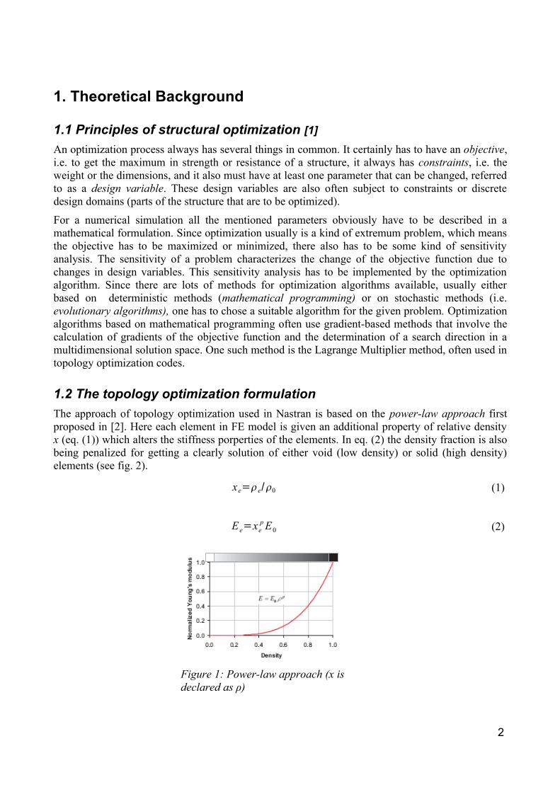
1.2 The topology optimization formulationThe approach of topology optimization used in Nastran is based on the power-law approach first proposed in [2]. Here each element in FE model is given an additional property of relative density x (eq. (1)) which alters the stiffness porperties of the elements. In eq. (2) the density fraction is also being penalized for getting a clearly solution of either void (low density) or solid (high density) elements (see fig. 2).
xe=e/0 (1)
E e=xep E0 (2)
2
Figure 1: Power-law approach (x is declared as ρ)
The objective of most common topology optimization problems is to find the minimum compliance c of a structure by a change in the distribution of mass or, in a fixed geometrie (volume), the distribution of densities. The objective function can therefore be defined as eq. (3).
c x =f Tu (3)
This compliance is the scalar product of the two vectors and resembles the work done by the force vector along the calculated displacements. Thus the given expression is actually a potential similar to common formulations for energy equilibria [...].Thereby the force vector f is equal to the resulting displacements of the finite elements analysis multiplied by the stiffness matrix with the current density distribution (eq. (4)).
K x u=f (4)
With some further transformation the objective function can be written as eq. (5) [3]. The compliance here is a linear combination of the compliances of each element.
min :c x =∑e=1
N
ueTk e xeue (5)
Since it is a normalized value, the design variable can only range between the values 0 (void) and 1 (solid) and therefore has to be restricted. For prevention of possible singularities in the system's matrices the densities are not restricted by zero but by a lower bound (eq. (6)).
gelow=xmin− xe0
geup= xe−10
(6)
Also, since this optimization method is basically a redistribution of material, the mass has to be constrained (eq. (7)).
h x=∑e=1
N
V e e−M 0=0 ⇔V x
V 0=const (7)
The complete topology optimization problem statement for minimizing compliance therefore reads as eq. (8) [4].
minx∈ℝn
{cx ∣h x=0,g low0,gup0} (8)
Although there are many optimization problems that can be solved with Nastran, this problem statement has been customized in Patran and can be easily used on a given geometry.
2. Computational Methodology
2.1 Optimization ParametersLike many other finite elements codes Nastran works with so-called input files that contain the commands which are to be performed. The input file always has to start with a SOL-command that calls the according solution sequence. In this case it is SOL200 for optimization problems. Furthermore the input file is divided in decks and cards. There are several decks containing execution parameters, parameters for different solution cases and information about meshing, geometry, loads etc. Each deck consists of several Cards which contain information for each parameter, like the point of application of a force, its magnitude, etc.
For an optimization problem several additional cards have to be written into the Nastran Input File.
3
Some basic parameters concerning topology optimization are to be mentioned in this context.
First of all, the design variables, which are to be changed in the course of the optimization, have to be defined. This can for example be done by the TOPVAR-entry (topology variable) that basically adds a density fraction property to the referenced elements. This possibility of direct definition of a TOPVAR-entry has only been recently added to the Nastran Code for topology optimization purposes [5]. Secondly, for each parameter that needs to be calculated in the course of optimization, a design response has to be defined. This is done by DRESPi-entries that can reference certain results, like the needed compliance of a structure. At last, there has to be a design objective function, referenced by the DESOBJ-card, and design constraints, like the fractional mass constraint. The latter are referenced by the DCONSTR-cards.
There are also many other parameters available, for example control commands the amount of performed design cycles, the convergence criteria, etc. For further information on Nastran input files and command decks, see the referenced Nastran user guides [5,6].
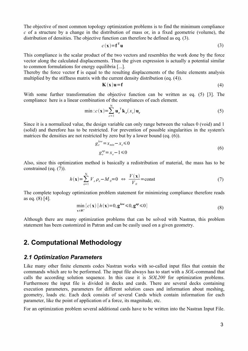
2.2 Optimization ProcessEvery optimization process in Nastran SOL200 consists on the basic steps shown in fig. 2. After initialisation, a first finite element analysis is performed as basis for the first optimization evaluation. Then, a new design is proposed, the design variables are updated and a convergence check, depending on the prior defined criteria, is performed. After the first cycle, this procedure will be repeated until the convergence criteria are fulfilled.
In MSC.Nastran several optimization libraries are available like BigDot or MSCADS. Both Codes might differ slightly in performance considering the nature of the optimization problem. For topology optimization the BigDot optimizer is recommended [5].
After the optimization process the results are written in a *.des-file that can be accessed by Patran for post-processing. Also, depending on the DESPCH-entry in the case control section, intermediate design responses can be accessed.
4
Figure 2: Computational flow diagram for optimization simulation with Nastran
3. Pre-Processing with PatranIn this case a simple model of a cantilever plate under a single-point load is used. The model is considered to be already available as displayed in fig.3, consisting of plate with the dimensions 30 x 10 x 1 mm3 and discretized by 60 x 20 isometric CQUAD4-elements. The material is considered as aluminum with a Young's modulus of 70 GPa and a Poisson's ratio of 0,3. A single point load of 20 N is applied to the lower outermost corner of the plate. The used parameters for the topology optimization are similar to those used for the basic problem in [7], since the nature of the problem is the same.
A. Set-up of topology optimization formulation– This step can easily be done with Patran in the
Analysis section. By chosing Action: Optimized, the Customized Solutions at the end of the window pane is accessible.
5
Figure 3: Finite Element Model
– Here, Use Customized Solutions has to be selected and the topology optimization parameters can be edited.
– a. Design Domain:
– Here, the desired property region for Topology optimization hast to be selected by clicking on the properties.
– For more complex structures manufacturing constraints can be added so that the designed structure is castable, for example (mold drafts, undercuts,..)[5].
– b. Objectives & Constraints:
– Analysis Discipline: Check Static. (The Normal Modes option can be used for a maximizing eigenvalue optimization problem that is also already implemented.)
– Objective Function is Minimize Compliance.
– Mass Target Constraint: Here, the target value for the mass fraction after the optimization process has to be entered. This value should match the initial density value, so the initial design is feasible [5]. Proposed is a value of 0.5, so the initial design is well balanced between the boundaries.
– c. Optimization Control Parameters:
6
abc
– Following Parameters are proposed:
– Initial Design (starting value of design variables): XINIT = 0.5.
– Maximum Design Cycles (can be varied): DESMAX = 20 (default).
– Penalty Factor (for design variables): POWER = 3.
– Move Limit (maximum change in design variables): DELXV=0.2.
– Tolerance of convergence (break criterion): CONV1=10E-4.
– Minimum member size (design filter suppressing the development of thin members in fine meshes [1,5], not needed with the given mesh): TDMIN=0.
– Checkboard-free Method (suppressing the checkerboard problem that might appear in topology optimization[1,5]): checked.
B. Optimization– It has to be verified that the correct subcase
with the correct solution sequence is selected. For the given problem statement the solution sequence SOL 101 LINEAR STATIC has to be selected.
– The analysis can be started by hitting the Apply-button.
7
4. Post-Processing with PatranAfter running the analysis, the results, i.e. the new density distribution or the displacement vector of the optimized structure, can be displayed with Patran. During the analysis, a *.des-file is created by Nastran that contains the information of the elements' density fractions. This file has to be loaded into Patran.
A. Display of density distribution– In the Menu Bar go to Tools -> Design Study
-> Post-process...
– In the appearing context window chose Read Results, Result Entities, select the corresponding results file (jobname.des) and hit the Apply-button.
– By changing the Action-scroll down window to Display Results, the density distribution can be displayed.
– The design cycle has to be selected.
– Only the elements with a density above the threshold value are displayed (Change this value for different images of the model).
– By checking Fringe, all elements are displayed, colored differently corresponding to their density fraction value.
8
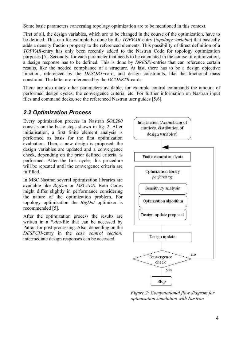
Resulting element density distribution for given problem. Left: All elements above a threshold of 0.3. Right: Fringe display (threshold: 0.0)
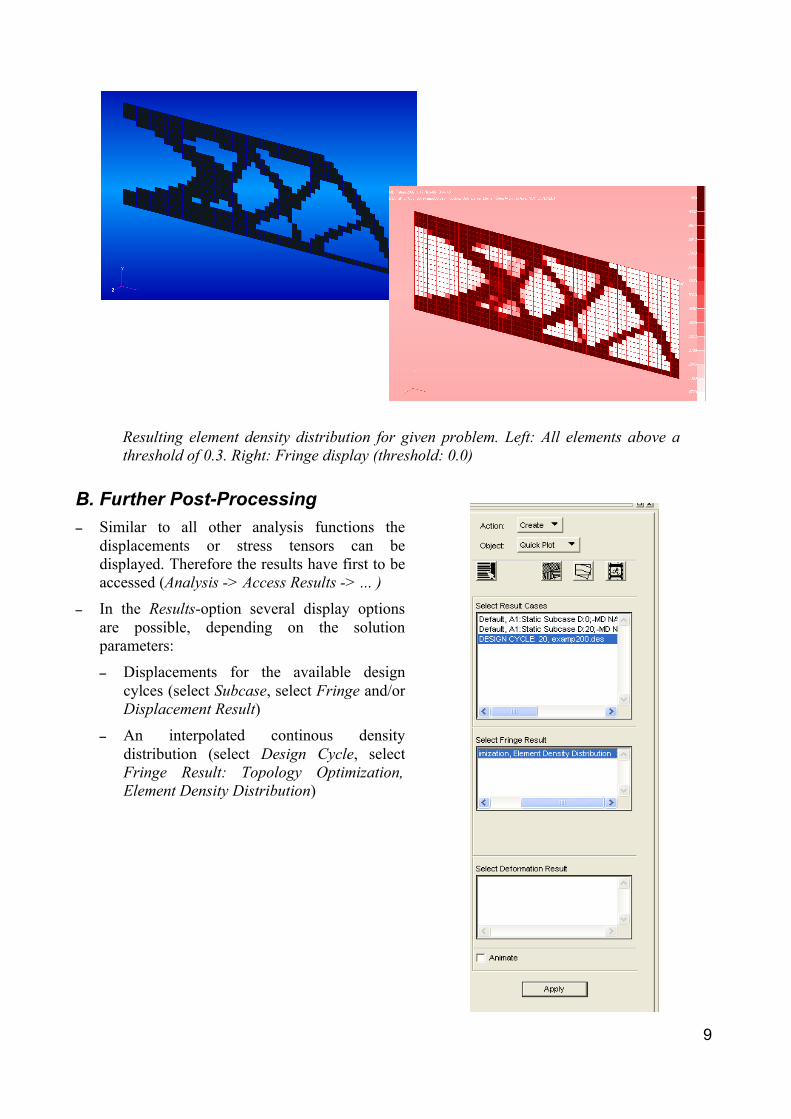
B. Further Post-Processing– Similar to all other analysis functions the
displacements or stress tensors can be displayed. Therefore the results have first to be accessed (Analysis -> Access Results -> ... )
– In the Results-option several display options are possible, depending on the solution parameters:
– Displacements for the available design cylces (select Subcase, select Fringe and/or Displacement Result)
– An interpolated continous density distribution (select Design Cycle, select Fringe Result: Topology Optimization, Element Density Distribution)
9
Left: Display of deformation of the given structure, Right: Display of continous density distribution.
5. Remarks– The presented solution is a readily customized solution for simple topology optimization
problems. For more complex solutions it is recommended to use the pre-processing under tools -> design study -> pre-process or hand-write the concerning parts of the Nastran input file (see Appendix). Hereby it is possible to define only certain regions for optimization or to define further responses or constraints.
– Further possible exercises:
– Compare results of analysis before and after optimization. By changing the solution sequence in the subcase selection context it is also possible to access other results, like eigenmodes, frequency responses, etc.
– Change fineness of the mesh. This will also change the results of the optimization. For a fine mesh the influence of the Minimum Member Size Constraint can also be observed.
– By adding the parameter DESPCH to the input file (see Appendix) intermediate designs can be accessed. (DESPCH = 4 means a printout every 4 cycles).
– Change loads or boundary constraints.
10
6. Literature[1] Pedersen, Pauli: Optimal Designs – Structures and Materials – Problems and Tools.
Departement of Mechanical Engineering, Solid Mechanics, Technical University of Denmark, 2003.
[2] Bendsoe, M.P.: Optimal Shape Design as a Material distribution problem. Structural and Multidisciplinary Optimization, Vol. 1:193-202, 1989.
[3] Bendsoe, M.P. And Sigmund, O.: Topology Optimization – Theory, Methods and Applications. Springer Verlag, Germany, 2003.
[4] Kress, G. and Keller, D.: Structural Optimisation, Zentrum für Strukturtechnologie, ETH Zürich, 2007
[5] MSC Nastran 2007 r1 – User's Guide pour Topology Optimization. The MSC Corporation, 2007.